Frobenius trace distributions for $K3$ surfaces

Abstract.

We study the distribution of the Frobenius traces on $K3$ surfaces. We compare experimental data with the predictions made by the Sato–Tate conjecture, i.e. with the theoretical distributions derived from the theory of Lie groups assuming equidistribution. Our sample consists of generic $K3$ surfaces, as well as of such having real and complex multiplication. Each time, the theoretical density and the histogram obtained by counting points match in the range of visible accuracy. Thus, we report evidence for the Sato–Tate conjecture for the surfaces considered.

1. Introduction

Given a smooth, projective variety $X$ over ${\mathbbm{Q}}$, one may choose a model ${\mathscr{X}}$ of $X$ that is projective over $\mathop{\text{\rm Spec}}\nolimits{\mathbbm{Z}}$. The point counts $\#{\mathscr{X}}_{p}({\mathbbm{F}}_{\!p})$, at least for the primes $p$ of good reduction, then form a highly interesting set of quantities related to the variety $X$. For example, for $X$ an elliptic curve, Hasse’s bound states that $a_{p}\in[-2,2]$, for $\smash{a_{p}:=(\#{\mathscr{X}}_{p}({\mathbbm{F}}_{\!p})-p-1)/\sqrt{p\mathstrut}}$, and it seems natural to ask for the distribution of the sequence $(a_{p})_{p\in{\mathbbm{P}}}$ in that interval.

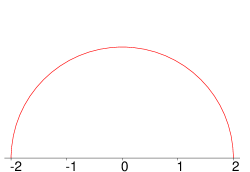
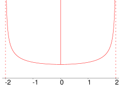
Figure 1. Distribution for elliptic curves, general (left) and CM (right)

When $X$ does not have CM, $(a_{p})_{p\in{\mathbbm{P}}}$ is equidistributed with respect to the measure with density $\smash{\frac{1}{2\pi}\sqrt{4-t^{2}}}$. This was first observed experimentally by M. Sato. J. Tate gave a partial explanation based on what is now called the Tate conjecture, applied to the direct powers $X^{m}$ [Tat, §4]. Making strong assumptions, related to modularity, on the elliptic curve, J.-P. Serre [Se68, §I.A.2, Example 3] provided a proof shortly afterwards. Based on new developments originating with A. Wiles [Wi], the result was finally established unconditionally by R. Taylor et al. [CHT, HST, Tay]. The CM case is substantially easier and was well understood already in the sixties. Here, the density function is $\smash{\frac{1}{\pi\sqrt{4-t^{2}}}}$. A proof may be found in [Su19, Proposition 2.16].

For curves of higher genus, extensive experiments have been carried out by A. Sutherland [Su19, KS]. Numerical data are available from his website [Su20]. Theoretical investigations concerning the genus-$2$ case are made in [FKRS]. An equidistribution statement is proven in certain cases, in which the Jacobian is geometrically isogenous to a direct product of elliptic curves, cf. [FS]. For an arbitrary smooth, projective variety $X$, there is the Sato–Tate conjecture, which we describe in Section 2. It is not just concerned with the traces, but predicts equidistribution of certain elements $x_{p}$ derived from the Frobenii within a compact Lie group, the Sato–Tate group $\mathop{\text{\rm ST}}\nolimits^{i}(X)$.

In the situation of a $K3$ surface, there is an explicit description of the neutral component $(\mathop{\text{\rm ST}}\nolimits^{2}(X))^{0}$ of the Sato–Tate group, due to the work of Yu. G. Zarhin [Za] and S. G. Tankeev [Tan90, Tan95]. In fact, $(\mathop{\text{\rm ST}}\nolimits^{2}(X))^{0}$ depends only on the geometric Picard rank, the degree of the endomorphism field $E$, and the bit of information whether $E$ is totally real or a CM field. We recall the description of $(\mathop{\text{\rm ST}}\nolimits^{2}(X))^{0}$ in Corollary 4.9.

Note that the concept of the endomorphism field is more subtle here than for abelian varieties, since one considers the endomorphism field of a Hodge structure associated with $X$. Cf. Paragraph 4.6 for details.

A theoretical result

For arbitrary $K3$ surfaces, we give an upper bound for the possible component groups of $\mathop{\text{\rm ST}}\nolimits^{2}(X)$ in Theorem 4.12. For example, in the case of real multiplication by a quadratic number field, $\smash{\mathop{\text{\rm ST}}\nolimits^{2}_{\text{\rm tr}}(X)/(\mathop{\text{\rm ST}}\nolimits^{2}(X))^{0}}$ is naturally contained in the dihedral group of order eight. We show that the order is, in fact, at most four and indicate that two non-isomorphic subgroups of order four are possible.

But this is not the main goal of this article. The main goal is to report on our experiments concerning the Sato–Tate conjecture for certain $K3$ surfaces of geometric Picard rank $16$ (and $17$). The surfaces in our sample have singular models of degree two and vary in endomorphism field and jump character [CEJ]. For every surface, we determine the Sato–Tate measure, i.e. the theoretical distribution of the Frobenius traces, according to the Sato–Tate conjecture, and compare it with a histogram obtained by explicitly counting points, for all primes $p$ up to $10^{8}$.

The experimental results

For any of the seven surfaces in our sample, the theoretical distribution and the histogram match in the range of visible accuracy. We present the seven histograms, each one in juxtaposition with the graph of the corresponding theoretical density function, in Section 5. Cf. Figures 2 to 5. The same information in higher resolution is available from the second author’s web page at https://www.uni-math.gwdg.de/jahnel/Arbeiten/histograms.tar.gz.

Concerning the rate of convergence, our data suggest that the order is $\smash{\frac{1}{2}}$. I.e., that the distribution of the Frobenius traces converges towards the Sato–Tate measure of order $\smash{\frac{1}{2}}$, in terms of the number of primes used. We present data supporting such a conjecture for one of our examples. The other surfaces show qualitatively the same behaviour.

The selection of our sample

Any selection of examples is, of course, somewhat arbitrary. However, we strongly feel that $K3$ surfaces of geometric Picard rank $16$ are a very reasonable compromise between surfaces of high rank, which are very special, and surfaces of low rank, which are certainly general, but hard to treat. Most notably, rank $16$ is the largest one that allows real multiplication [vG, Lemma 3.2].

We include an example of geometric Picard rank $17$ and trivial jump character, as, in this situation, the theoretical density function is not symmetric. Cf. the third histogram in Figure 2.

Computations

The computations related to this project were done with magma [BCP]. For symbolic integration, we used maple [Ma].

2. The Sato–Tate conjecture

The algebraic monodromy group

Let $X$ be a smooth, projective variety over ${\mathbbm{Q}}$, and $S$ a finite set of primes, outside of which $X$ has good reduction. Then the Lefschetz trace formula in étale cohomology [SGA5, Exposé III, Théorème 6.13.3], together with the smooth specialisation theorem [SGA4, Exposé XVI, Corollaire 2.2], show

$$\#{\mathscr{X}}_{p}({\mathbbm{F}}_{\!p})=\!\sum_{i=0}^{2\dim X}\!\!(-1)^{i}\,\text{\rm Tr}\big{(}\!\mathop{\text{\rm Frob}}\nolimits_{p}\colon H_{\text{\rm\'{e}t}}^{i}(X_{\overline{\mathbbm{Q}}},{\mathbbm{Q}}_{l})\righttoleftarrow\!\big{)}\,,$$ (1)

for $p\in{\mathbbm{P}}\setminus S$ and any prime $l\neq p$. Here, $\mathop{\text{\rm Frob}}\nolimits_{p}\in\mathop{\text{\rm Gal}}\nolimits(\overline{\mathbbm{Q}}/{\mathbbm{Q}})$ denotes a Frobenius lift. Since $\mathop{\text{\rm Frob}}\nolimits_{p}$ is unique up to conjugation, the trace is independent of that choice.

Suppose now that $i$ is even, which is the slightly easier case and the one we study in this article. Then

$$\text{\rm Tr}\big{(}\!\mathop{\text{\rm Frob}}\nolimits_{p}\colon H_{\text{\rm\'{e}t}}^{i}(X_{\overline{\mathbbm{Q}}},{\mathbbm{Q}}_{l})\righttoleftarrow\!\big{)}=p^{\frac{i}{2}}\!\cdot\text{\rm Tr}\big{(}\!\mathop{\text{\rm Frob}}\nolimits_{p}\colon H_{\text{\rm\'{e}t}}^{i}(X_{\overline{\mathbbm{Q}}},{\mathbbm{Q}}_{l}(i/2))\righttoleftarrow\!\big{)}\,.$$ (2)

The trace on the right hand side is known to be a rational number that is independent of $l$. According to the Weil conjectures, proven by P. Deligne [De74, Théorème 1.6], every eigenvalue of $\mathop{\text{\rm Frob}}\nolimits_{p}$ is an algebraic number, all complex (and real) embeddings of which are of absolute value $1$.

Moreover, the operation of the Galois group,

$$\varrho^{i}_{X,l}\colon\mathop{\text{\rm Gal}}\nolimits(\overline{\mathbbm{Q}}/{\mathbbm{Q}})\longrightarrow\mathop{\text{\rm GL}}\nolimits(H_{\text{\rm\'{e}t}}^{i}(X_{\overline{\mathbbm{Q}}},{\mathbbm{Q}}_{l}(i/2)))\,,$$ (3)

is continuous, cf. [SGA4, Exposé VIII, Théorème 5.2]. Its image is hence an $l$-adic Lie group. The Zariski closure $\smash{G_{X,l}^{i,\text{\rm Zar}}:=\overline{\mathop{\text{\rm im}}\nolimits(\varrho^{i}_{X,l})}}$ is called the algebraic monodromy group of $X$ (in degree $i$). It is a linear algebraic group over ${\mathbbm{Q}}_{l}$.

Inclusion in the orthogonal group

Fix a hyperplane section $H\subset X$. Then, by Poincaré duality and the hard Lefschetz theorem [De80, Théorème 4.1.1], the cohomology vector space $H_{\text{\rm\'{e}t}}^{i}(X_{\overline{\mathbbm{Q}}},{\mathbbm{Q}}_{l}(i/2))$ is equipped with a non-degenerate, symmetric, bilinear pairing. For $i\leq\dim X$, this is given as follows,

$$H_{\text{\rm\'{e}t}}^{i}(X_{\overline{\mathbbm{Q}}},{\mathbbm{Q}}_{l}(i/2))\times H_{\text{\rm\'{e}t}}^{i}(X_{\overline{\mathbbm{Q}}},{\mathbbm{Q}}_{l}(i/2)) \longrightarrow H_{\text{\rm\'{e}t}}^{2\dim X}(X_{\overline{\mathbbm{Q}}},{\mathbbm{Q}}_{l}(\dim X))\cong{\mathbbm{Q}}_{l}\,,$$

$$(\alpha,\beta) \mapsto \langle\alpha,\beta\rangle:=\alpha\cup\beta\cup[H]^{\dim X-i}\,.$$

The operation of $\mathop{\text{\rm Gal}}\nolimits(\overline{\mathbbm{Q}}/{\mathbbm{Q}})$ respects this pairing, so one actually has an inclusion

$$G_{X,l}^{i,\text{\rm Zar}}\subseteq\mathop{\text{\rm O}}\nolimits(H_{\text{\rm\'{e}t}}^{i}(X_{\overline{\mathbbm{Q}}},{\mathbbm{Q}}_{l}(i/2)))\,.$$

The Sato–Tate group

Let us fix an embedding ${\mathbbm{Q}}_{l}\hookrightarrow{\mathbbm{C}}$. Then $\smash{G_{X,l}^{i,\text{\rm Zar}}({\mathbbm{C}})}$ is a complex Lie group, equipped with an inclusion $\smash{\iota\colon G_{X,l}^{i,\text{\rm Zar}}\hookrightarrow G_{X,l}^{i,\text{\rm Zar}}({\mathbbm{C}})}$. Moreover, $\smash{G_{X,l}^{i,\text{\rm Zar}}({\mathbbm{C}})}$ is contained in the matrix group $\mathop{\text{\rm O}}\nolimits(H_{\text{\rm\'{e}t}}^{i}(X_{\overline{\mathbbm{Q}}},{\mathbbm{Q}}_{l}(i/2))\otimes_{{\mathbbm{Q}}_{l}}\!{\mathbbm{C}})$. In particular, the elements of $\smash{G_{X,l}^{i,\text{\rm Zar}}({\mathbbm{C}})}$ have eigenvalues being complex numbers and there is the trace map

$$\text{\rm tr}\colon G_{X,l}^{i,\text{\rm Zar}}({\mathbbm{C}})\to{\mathbbm{C}}\,.$$

The maximal compact subgroup $\mathop{\text{\rm ST}}\nolimits^{i}(X)$ of $\smash{G_{X,l}^{i,\text{\rm Zar}}({\mathbbm{C}})}$ is called the Sato–Tate group of $X$ in degree $i$. The Sato–Tate group is a compact Lie group, in general disconnected. For the component group, one clearly has

$$\mathop{\text{\rm ST}}\nolimits^{i}(X)/(\mathop{\text{\rm ST}}\nolimits^{i}(X))^{0}\cong G_{X,l}^{i,\text{\rm Zar}}({\mathbbm{C}})/(G_{X,l}^{i,\text{\rm Zar}}({\mathbbm{C}}))^{0}\cong G_{X,l}^{i,\text{\rm Zar}}/(G_{X,l}^{i,\text{\rm Zar}})^{0}\,.$$

Remarks 2.1.

• The maximal compact subgroups of a Lie group with finitely many connected components are mutually conjugate [OV, Theorem IV.3.5]. Thus, the Sato–Tate group is well-defined, up to conjugation.

• According to the Mumford–Tate conjecture, the neutral component $\smash{(G_{X,l}^{i,\text{\rm Zar}})^{0}}$ of the algebraic monodromy group $\smash{G_{X,l}^{i,\text{\rm Zar}}}$ coincides with $\mathop{\text{\rm Hg}}\nolimits^{i}(X)\!\times_{\mathop{\text{\rm Spec}}\nolimits{\mathbbm{Q}}}\!\mathop{\text{\rm Spec}}\nolimits{\mathbbm{Q}}_{l}$, for $\mathop{\text{\rm Hg}}\nolimits^{i}(X)$ the $i$-the Hodge group of $X$ [Su19, Definition 3.8 and Conjecture 3.10].

Remark 2.2.

One might want to work without Tate twist, as one is forced to do in the case when $i$ is odd. The algebraic monodromy group is then only contained in $\mathop{\text{\rm GO}}\nolimits(H_{\text{\rm\'{e}t}}^{i}(X_{\overline{\mathbbm{Q}}},{\mathbbm{Q}}_{l}))$ and one would impose an orthogonal constraint, i.e. intersect with the orthogonal group, afterwards. Cf. [Su19], in particular [Su19, Remark 3.3].

Such an approach is, however, inferior to the one with Tate twist in the case of even $i$, at least as far as the component groups are considered. For example, the algebraic monodromy group might be $[\mathop{\text{\rm SO}}\nolimits_{3}({\mathbbm{Q}}_{l})]^{2}$. Then, working without Tate twist, one would find, at first, $\mathop{\text{\rm G}}\nolimits[\mathop{\text{\rm SO}}\nolimits_{3}({\mathbbm{Q}}_{l})]^{2}$. In the next step, however, this leads to $\mathop{\text{\rm G}}\nolimits[\mathop{\text{\rm SO}}\nolimits_{3}({\mathbbm{Q}}_{l})]^{2}\cap\mathop{\text{\rm O}}\nolimits_{6}({\mathbbm{Q}}_{l})=[\mathop{\text{\rm SO}}\nolimits_{3}({\mathbbm{Q}}_{l})]^{2}\cup[\mathop{\text{\rm O}}\nolimits_{3}^{-}({\mathbbm{Q}}_{l})]^{2}$, in which, all of a sudden, a second component appears. In other words, some of the information has been lost.

The Sato–Tate conjecture

The set $\mathop{\text{\rm Cl}}\nolimits(\mathop{\text{\rm ST}}\nolimits^{i}(X))$ of the conjugacy classes of elements of $\mathop{\text{\rm ST}}\nolimits^{i}(X)$ naturally carries the quotient topology with respect to the canonical map $\pi\colon\mathop{\text{\rm ST}}\nolimits^{i}(X)\to\mathop{\text{\rm Cl}}\nolimits(\mathop{\text{\rm ST}}\nolimits^{i}(X))$. As $\smash{\text{\rm tr}|_{\mathop{\text{\rm ST}}\nolimits^{i}(X)}\colon\mathop{\text{\rm ST}}\nolimits^{i}(X)\to{\mathbbm{C}}}$ is a continuous class function, it induces a continuous map $\text{\rm tr}^{\prime}\colon\mathop{\text{\rm Cl}}\nolimits(\mathop{\text{\rm ST}}\nolimits^{i}(X))\to{\mathbbm{C}}$ satisfying $\smash{\text{\rm tr}^{\prime}\!\circ\!\pi=\text{\rm tr}|_{\mathop{\text{\rm ST}}\nolimits^{i}(X)}}$. One equips $\mathop{\text{\rm Cl}}\nolimits(\mathop{\text{\rm ST}}\nolimits^{i}(X))$ with the measure $\pi_{*}\mu_{\text{\rm Haar}}$, for $\mu_{\text{\rm Haar}}$ the normalised Haar measure on $\mathop{\text{\rm ST}}\nolimits^{i}(X)$.

Moreover, for an arbitrary $p\in{\mathbbm{P}}\setminus S$, one puts

$$\xi_{p}:=\iota(\varrho^{i}_{X,l}(\mathop{\text{\rm Frob}}\nolimits_{p}))\in G_{X,l}^{i,\text{\rm Zar}}({\mathbbm{C}})\,.$$

This element is uniquely determined, up to conjugation. Write $\xi_{p}^{\text{\rm ss}}$ for the semisimple part of $\xi_{p}$, according to the Jordan decomposition [Bo, Theorem I.4.4]. Then all eigenvalues of $\smash{\xi_{p}^{\text{\rm ss}}}$ are of absolute value $1$. Thus, the group $\smash{\langle\xi_{p}^{\text{\rm ss}}\rangle\subset G_{X,l}^{i,\text{\rm Zar}}({\mathbbm{C}})}$ has a compact closure. By [OV, Theorem IV.3.5], $\smash{\langle\xi_{p}^{\text{\rm ss}}\rangle}$ is, up to conjugation, contained in $\mathop{\text{\rm ST}}\nolimits^{i}(X)$. Let, finally,

$$x_{p}\in\mathop{\text{\rm Cl}}\nolimits(\mathop{\text{\rm ST}}\nolimits^{i}(X))$$

be the conjugacy class of $\xi_{p}^{\text{\rm ss}}$. Lemma 2.8 below shows that $x_{p}$ is well-defined.

Conjecture 2.3 (The Sato–Tate conjecture).

Let $X$ and $i$ be as above. Then the sequence $(x_{p})_{p\in{\mathbbm{P}}\setminus S}$, for $p$ running through the good primes in their usual order, is equidistributed with respect to $\pi_{*}\mu_{\text{\rm Haar}}$. In other words, the sequence $\big{(}\frac{1}{\#\{q\in{\mathbbm{P}}\setminus S\mid q\leq p\}}\!\!\sum\limits_{\genfrac{}{}{0.0pt}{}{q\in{\mathbbm{P}}\setminus S}{q\leq p}}\!\!\delta_{x_{q}}\big{)}_{p\in{\mathbbm{P}}}$ of measures on $\mathop{\text{\rm Cl}}\nolimits(\mathop{\text{\rm ST}}\nolimits^{i}(X))$ converges weakly versus $\pi_{*}\mu_{\text{\rm Haar}}$.

Remarks 2.4.

• (Equidistribution on the component group.) In particular, the Sato–Tate conjecture claims equidistribution among the components of $\mathop{\text{\rm ST}}\nolimits^{i}(X)$.

  More precisely, let $\mu_{\text{\rm un}}$ be the uniform probability measure on the component group $\mathop{\text{\rm ST}}\nolimits^{i}(X)/(\mathop{\text{\rm ST}}\nolimits^{i}(X))^{0}$. Moreover, let $\pi_{c}\colon\mathop{\text{\rm ST}}\nolimits^{i}(X)/(\mathop{\text{\rm ST}}\nolimits^{i}(X))^{0}\to\mathop{\text{\rm Cl}}\nolimits(\mathop{\text{\rm ST}}\nolimits^{i}(X)/(\mathop{\text{\rm ST}}\nolimits^{i}(X))^{0})$ be the canonical map and $\kappa_{c}\colon\mathop{\text{\rm Cl}}\nolimits(\mathop{\text{\rm ST}}\nolimits^{i}(X))\to\mathop{\text{\rm Cl}}\nolimits(\mathop{\text{\rm ST}}\nolimits^{i}(X)/(\mathop{\text{\rm ST}}\nolimits^{i}(X))^{0})$ the map between conjugacy classes induced by the projection $\kappa\colon\mathop{\text{\rm ST}}\nolimits^{i}(X)\to\mathop{\text{\rm ST}}\nolimits^{i}(X)/(\mathop{\text{\rm ST}}\nolimits^{i}(X))^{0}$. Then $(\kappa_{c}(x_{p}))_{p\in{\mathbbm{P}}\setminus S}$ is asserted to be equidistributed with respect to $(\pi_{c})_{*}\mu_{\text{\rm un}}$. Indeed,

  $$(\kappa_{c})_{*}\pi_{*}\mu_{\text{\rm Haar}}=(\kappa_{c}\!\circ\!\pi)_{*}\mu_{\text{\rm Haar}}=(\pi_{c}\!\circ\!\kappa)_{*}\mu_{\text{\rm Haar}}=(\pi_{c})_{*}\kappa_{*}\mu_{\text{\rm Haar}}=(\pi_{c})_{*}\mu_{\text{\rm un}}\,.\vspace{2mm}$$

  This part of the Sato–Tate conjecture is known to be true and can be shown as follows. The image of $\smash{\varrho^{i}_{X,l}\colon\mathop{\text{\rm Gal}}\nolimits(\overline{\mathbbm{Q}}/{\mathbbm{Q}})\to G_{X,l}^{i,\text{\rm Zar}}}$ is Zariski dense, hence the induced homomorphism

  $$\mathop{\text{\rm Gal}}\nolimits(\overline{\mathbbm{Q}}/{\mathbbm{Q}})\longrightarrow G_{X,l}^{i,\text{\rm Zar}}/(G_{X,l}^{i,\text{\rm Zar}})^{0}\cong\mathop{\text{\rm ST}}\nolimits^{i}(X)/(\mathop{\text{\rm ST}}\nolimits^{i}(X))^{0}$$

  is surjective. The kernel $U\subseteq\mathop{\text{\rm Gal}}\nolimits(\overline{\mathbbm{Q}}/{\mathbbm{Q}})$ is an open subgroup, so corresponding under the Galois correspondence there is a finite extension field $\smash{L_{0}\supseteq{\mathbbm{Q}}}$. I.e., $\smash{\varrho^{i}_{X,l}}$ yields an isomorphism $\smash{\mathop{\text{\rm Gal}}\nolimits(L_{0}/{\mathbbm{Q}})\cong\mathop{\text{\rm ST}}\nolimits^{i}(X)/(\mathop{\text{\rm ST}}\nolimits^{i}(X))^{0}}$. Consequently, the Chebotarev density theorem implies exactly what was claimed.

• (The $0$-dimensional case.) In particular, the Sato–Tate conjecture is trivially true when $(\mathop{\text{\rm ST}}\nolimits^{i}(X))^{0}$ is the trivial group. For example, this holds for $X$ of dimension $0$ and $i=0$. Indeed, then $\smash{H^{0}_{\text{\rm\'{e}t}}(X_{\overline{\mathbbm{Q}}},{\mathbbm{Q}}_{l})\cong{\mathbbm{Q}}_{l}^{\#\pi_{0}(X_{\overline{\mathbbm{Q}}})}}$ and $\mathop{\text{\rm Gal}}\nolimits(\overline{\mathbbm{Q}}/{\mathbbm{Q}})$ acts simply by permuting the direct summands. Consequently, the algebraic monodromy group $\smash{G_{X,l}^{0,\text{\rm Zar}}}$ must be finite.

• (Modularity.) For a representation $\varrho\colon\mathop{\text{\rm ST}}\nolimits^{i}(X)\to\mathop{\text{\rm GL}}\nolimits_{d}({\mathbbm{C}})$, consider the Artin type $L$-function

  $$L(\varrho,s):=\prod_{p\in{\mathbbm{P}}\setminus S}\frac{1}{\det(1-\varrho(x_{p})p^{-s})}\,,$$

  which is clearly holomorphic for $\mathop{\text{\rm Re}}\nolimits s>1$. Assume that, for every irreducible, continuous representation $\varrho\neq 1$ of $\mathop{\text{\rm ST}}\nolimits^{i}(X)$, the function $L(\varrho,s)$ extends to the closed half plane $\mathop{\text{\rm Re}}\nolimits s\geq 1$ as a continuous function not having any zeroes (or poles). Then the Sato–Tate conjecture is known to hold for $X$ and $i$ [Se68, §I.A.2, Theorem 2].

• (Cohomology.) The group $\mathop{\text{\rm Gal}}\nolimits(\overline{\mathbbm{Q}}/{\mathbbm{Q}})$ is compact and hence carries a normalised Haar measure itself. The conjugacy classes of $\mathop{\text{\rm Frob}}\nolimits_{p}$, for $p$ running through the primes in their usual order, are equidistributed with respect to this Haar measure, according to the Chebotarev density theorem. As the representation $\smash{\varrho^{i}_{X,l}}$ is continuous, the image $\smash{\mathop{\text{\rm im}}\nolimits\varrho^{i}_{X,l}}$ is compact, and the conjugacy classes of $\smash{\varrho^{i}_{X,l}(\mathop{\text{\rm Frob}}\nolimits_{p})}$ are equidistributed with respect to the normalised Haar measure on that $l$-adic Lie group. This $l$-adic kind of equidistribution is certainly of interest. For example, it was studied in detail, for elliptic curves, by J.-P. Serre in [Se72]. However, as the embedding ${\mathbbm{Q}}_{l}\hookrightarrow{\mathbbm{C}}$ chosen is discontinuous, it does not seem to have any implications towards the Sato–Tate conjecture. A cohomology theory with coefficients in ${\mathbbm{C}}$ that provides a continuous $\mathop{\text{\rm Gal}}\nolimits(\overline{\mathbbm{Q}}/{\mathbbm{Q}})$-action would certainly help. But, of course, we have nothing of this kind at our disposal.

Remark 2.5.

When $X$ is a $K3$ surface, which is the situation we are interested in in this article, $\xi_{p}$ is known to be semisimple, for every good prime $p\neq l$ [De81, Corollaire 1.10]. The step of taking the semisimple part is then superfluous.

The Sato–Tate conjecture immediately yields the following prediction for the distribution of the Frobenius traces.

Conjecture 2.6 (The Frobenius trace distribution).

Let $X$ and $i$ be as above. Then the sequence $\smash{\text{\rm Tr}(\mathop{\text{\rm Frob}}\nolimits_{p})_{p\in{\mathbbm{P}}\setminus S}}$, for $p$ running through the good primes in their usual order, is equidistributed with respect to $(\text{\rm tr}|_{\mathop{\text{\rm ST}}\nolimits^{i}(X)})_{*}\mu_{\text{\rm Haar}}$. In other words, the sequence

$$\textstyle\big{(}\frac{1}{\#\{q\in{\mathbbm{P}}\setminus S\mid q\leq p\}}\!\!\sum\limits_{\genfrac{}{}{0.0pt}{}{q\in{\mathbbm{P}}\setminus S}{q\leq p}}\!\!\delta_{\text{\rm Tr}(\mathop{\text{\rm Frob}}\nolimits_{q})}\big{)}_{p\in{\mathbbm{P}}}$$

of measures on ${\mathbbm{R}}$ is convergent in the weak sense versus $(\text{\rm tr}|_{\mathop{\text{\rm ST}}\nolimits^{i}(X)})_{*}\mu_{\text{\rm Haar}}$.

Proof (assuming the Sato–Tate conjecture). Taking the image measure under a continuous map commutes with weak convergence, cf. [Di, section 13.4, problème 8]. Hence, the Sato–Tate conjecture implies that

$$\textstyle\frac{1}{\#\{q\in{\mathbbm{P}}\setminus S\mid q\leq p\}}\!\!\sum\limits_{\genfrac{}{}{0.0pt}{}{q\in{\mathbbm{P}}\setminus S}{q\leq p}}\!\!\delta_{\text{\rm tr}^{\prime}(x_{q})}=\text{\rm tr}^{\prime}_{*}\big{(}\frac{1}{\#\{q\in{\mathbbm{P}}\setminus S\mid q\leq p\}}\!\!\sum\limits_{\genfrac{}{}{0.0pt}{}{q\in{\mathbbm{P}}\setminus S}{q\leq p}}\!\!\delta_{x_{q}}\big{)} \to\text{\rm tr}^{\prime}_{*}(\pi_{*}\mu_{\text{\rm Haar}})$$

$$=(\text{\rm tr}^{\prime}\!\circ\!\pi)_{*}\mu_{\text{\rm Haar}}=(\text{\rm tr}|_{\mathop{\text{\rm ST}}\nolimits^{i}(X)})_{*}\mu_{\text{\rm Haar}}\,.$$

But $\smash{\text{\rm tr}^{\prime}(x_{q})=\text{\rm tr}^{\prime}(\pi(\xi_{q}))=\text{\rm tr}(\xi_{q})=\text{\rm tr}(\iota(\varrho^{i}_{X,l}(\mathop{\text{\rm Frob}}\nolimits_{p})))}$, for every prime number $q$. And $\smash{\text{\rm tr}(\iota(\varrho^{i}_{X,l}(\mathop{\text{\rm Frob}}\nolimits_{p})))=\text{\rm Tr}(\varrho^{i}_{X,l}(\mathop{\text{\rm Frob}}\nolimits_{p}))}$, which is usually denoted shortly as $\text{\rm Tr}(\mathop{\text{\rm Frob}}\nolimits_{p})$.   $\square$

A related conjecture – Lang–Trotter for general varieties

Let, as before, $X$ be a smooth, projective variety over ${\mathbbm{Q}}$, and $S$ a finite set of primes, outside of which $X$ has good reduction. Fix some $i\in{\mathbbm{N}}$. Then, for any $a\in{\mathbbm{Z}}$, one may ask for the asymptotics of

$$N^{i}_{X,a}(p):=\#\{q\in{\mathbbm{P}}\setminus S\mid q\leq p,\text{\rm Tr}(\mathop{\text{\rm Frob}}\nolimits_{q}\colon H_{\text{\rm\'{e}t}}^{i}(X_{\overline{\mathbbm{Q}}},{\mathbbm{Q}}_{l})\righttoleftarrow)=a\}\,,$$ (4)

for $p\to\infty$. Note that, as the cohomology vector space without Tate twist is considered, the traces of the Frobenii in (4) are automatically integers.

Formula (2) shows that, in the notation used above, the second condition in the definition of $N^{i}_{X,a}(p)$ means $\smash{\text{\rm Tr}(\mathop{\text{\rm Frob}}\nolimits_{q})=\frac{a}{q^{i/2}}}$, or

$$\textstyle\smash{\text{\rm Tr}(\mathop{\text{\rm Frob}}\nolimits_{q})\in\left[\frac{a-\frac{1}{2}}{q^{i/2}},\frac{a+\frac{1}{2}}{q^{i/2}}\right]}\,.$$

Thus, assuming that the Sato–Tate measure $(\text{\rm tr}|_{\mathop{\text{\rm ST}}\nolimits^{i}(X)})_{*}\mu_{\text{\rm Haar}}$ has a density function whose limit for $t\to 0$ exists and is positive, it seems reasonable to expect, at least for $a\neq 0$, that there is a constant $C^{i}_{X,a}\geq 0$ such that

$$N^{i}_{X,a}(p)\sim C^{i}_{X,a}\!\cdot\!\!\sum_{\genfrac{}{}{0.0pt}{}{q\in{\mathbbm{P}}\setminus S}{q\leq p}}\!\frac{1}{q^{i/2}}\,.$$

I.e., that $N^{i}_{X,a}(p)=O(1)$, for $i>2$, and

$$N^{i}_{X,a}(p)\sim\left\{\begin{array}[]{ll}C^{i}_{X,a}\!\cdot\!\frac{2\sqrt{p}}{\log p}\,,&{\rm~{}for\;}i=1\,,\\ C^{i}_{X,a}\!\cdot\!\log\log p\,,&{\rm~{}for\;}i=2\,.\\ \end{array}\right.$$ (5)

In the case that the density is continuous and non-vanishing at $0$, one might hope for the same when $a=0$. This was formulated first, as a conjecture for elliptic curves and $i=1$, by S. Lang and H. Trotter [LT].

The case of a $K3$ surface

For $K3$ surfaces and $i=2$, which is the case we are interested in in this article, it seems that such a conjecture has not been explicitly stated before. Note, however, the somewhat optimistic discussion on page 2 of the article [CT] of E. Costa and Yu. Tschinkel.

Anyway, we are very reluctant to claim evidence in any nontrivial situation, as the experiments described in this article involve a search bound of $10^{8}$, which is a bit too low in order to detect double logarithmic growth.

There are, however, cases, in which (5) is trivially true. For instance, let $X$ be one of the surfaces from Examples 5.4 to 5.7, below. Then, for $a$ even, (5) holds with $C^{2}_{X,a}=0$. Indeed, a double cover of $\smash{{\text{\bf P}}^{2}_{{\mathbbm{F}}_{\!p}}}$, ramified over six ${\mathbbm{F}}_{\!p}$-rational lines in general position, always has an odd number of ${\mathbbm{F}}_{\!p}$-rational points, simply because the branch locus has. For a refinement of this argument taking $(a\bmod 4)$ into consideration, cf. [EJ22].

Remark 2.7.

One might expect an asymptotics similar to (5) for the primes of reduction to geometric Picard rank $22$. Again, this is certainly subject to restrictions, such as the occurrence of a continuous density function for the Sato–Tate measure. Note, for instance, that the $K3$ surfaces presented in [CEJ, Examples 2.6.5 and 2.6.7] reduce to geometric Picard rank $22$ at exactly half the primes.

A result from the theory of Lie groups

Due to the lack of a suitable reference, we include the following purely Lie-theoretic lemma.

Lemma 2.8.

Let $G$ be a faithfully representable complex Lie group and $K\subset G$ a maximal compact subgroup. Then the natural homomorphism $\mathop{\text{\rm Cl}}\nolimits K\to\mathop{\text{\rm Cl}}\nolimits G$ between conjugacy classes of elements is injective.

Proof. Let $k_{1},k_{2}\in K$ be two elements that are conjugate as elements of $G$. We have to show that $k_{1}$ and $k_{2}$ are conjugate in $K$.

According to the decomposition theorem [Le, Theorem 4.43], $G\cong G^{\prime}\!\ltimes\!R$ is isomorphic to a semidirect product of two closed subgroups, $R$ being simply connected and solvable and $G^{\prime}$ being reductive. A simply connected solvable group has the trivial group as its maximal compact subgroup [Kn, Corollary 1.126]. Thus, the quotient homomorphism $\pi\colon G\twoheadrightarrow G/R$ maps $K$ isomorphically onto the maximal compact subgroup of $G/R$. Moreover, the elements $\pi(k_{1})$ and $\pi(k_{2})$ are clearly conjugate in $G/R\cong G^{\prime}$.

It therefore suffices to assume $G$ as being reductive. Then $G$ coincides with the complexification of $K$ [Le, Theorem 4.31] and there is the Cartan decomposition $G=K\!\cdot\exp(i\mathop{\text{\rm Lie}}\nolimits K)$, cf. [Kn, Theorem 6.31.c)]. By assumption, there exist some $k\in K$ and $X\in\mathop{\text{\rm Lie}}\nolimits K$ such that $\exp(-iX)k^{-1}\!\cdot\!k_{1}\!\cdot\!k\exp(iX)=k_{2}\in K$. As $K$ is fixed under the Cartan involution $\Theta$, this yields

$$\exp(iX)\underline{k}\exp(-iX)=\Theta(\exp(-iX)\underline{k}\exp(iX))=\exp(-iX)\underline{k}\exp(iX)\,,$$

for $\underline{k}:=k^{-1}k_{1}k$. I.e., $\exp(2iX)\in\mathop{\text{\rm C}}\nolimits_{G}(\underline{k})$. Consequently, $\exp(2niX)\in\mathop{\text{\rm C}}\nolimits_{G}(\underline{k})$ for every $n\in{\mathbbm{Z}}$, which implies $\exp(tiX)\in\mathop{\text{\rm C}}\nolimits_{G}(\underline{k})$ for every $t\in{\mathbbm{R}}$ [Kn, Lemma 1.142]. In particular, $\exp(iX)\in\mathop{\text{\rm C}}\nolimits_{G}(\underline{k})$ showing $k^{-1}k_{1}k=k_{2}$, as required.  $\square$

3. Trace distributions for compact Lie groups

Moment sequences

Given a connected compact Lie group $S\subset\mathop{\text{\rm GL}}\nolimits_{d}({\mathbbm{C}})$, the trace $\text{\rm tr}|_{S}\colon S\to{\mathbbm{C}}$ is a continuous class function. Let us assume that $\text{\rm tr}|_{S}$ is real-valued. Then, for the $n$-th moment

$$\mathop{\text{\rm E}}\nolimits_{S}[\text{\rm tr}^{n}]=\int_{\mathbbm{R}}\!x^{n}\,d(\text{\rm tr}|_{S})_{*}\mu_{\text{\rm Haar}}(x)=\int_{S}\text{\rm tr}^{n}(s)\,d\mu_{\text{\rm Haar}}(s)\,,$$

for $n\in{\mathbbm{N}}$, one has the Weyl integration formula [Kn, Theorem 8.60],

$$\mathop{\text{\rm E}}\nolimits_{S}[\text{\rm tr}^{n}]=\frac{1}{\#W}\int_{T}\text{\rm tr}^{n}(t)\det(\text{\rm id}-\mathop{\text{\rm Ad}}\nolimits_{S/T}(t^{-1}))\,dt=\frac{1}{\#W}\int_{T}\text{\rm tr}^{n}(t)\!\prod_{\alpha\in\Delta^{+}}\!\!|1-t^{\alpha}|^{2}\,dt\,.$$

Here, $T$ denotes the maximal torus of $S$, $W$ the Weyl group, $\Delta^{+}$ a system of positive roots, and $\mathop{\text{\rm Ad}}\nolimits\colon T\to\mathop{\text{\rm GL}}\nolimits(S/T)$ the adjoint representation. The integrand is a trigonometric polynomial, so, for each $n$, the integral may be computed exactly.

The particular compact Lie groups mentioned in Table 1 are related to the examples of $K3$ surfaces that we present in this article, cf. Section 5.

Examples A

$S$	Root	$\dim(T)$	$\dim(S/T)$	Moment sequence	Label in
	system				[OEIS]
$\mathop{\text{\rm SO}}\nolimits_{2}({\mathbbm{R}})\cong\mathop{\text{\rm U}}\nolimits_{1}$	$\emptyset$	1	0	1, 0, 2, 0, 6, 0, 20,	A126869
				0, 70, 0, 252
$\mathop{\text{\rm SO}}\nolimits_{3}({\mathbbm{R}})$	$A_{1}$	1	2	1, 0, 1, 1, 3, 6, 15,	A005043
				36, 91, 232, 603
$\mathop{\text{\rm SO}}\nolimits_{5}({\mathbbm{R}})$	$B_{2}$	2	8	1, 0, 1, 0, 3, 1, 15,	A095922
				15, 105, 190, 945
$\mathop{\text{\rm SO}}\nolimits_{6}({\mathbbm{R}})$	$A_{3}$	3	12	1, 0, 1, 0, 3, 0, 16,	A247591
				0, 126, 0, 1296
$\mathop{\text{\rm U}}\nolimits_{3}$	$A_{2}^{\prime}$	3	6	1, 0, 2, 0, 12, 0, 120,	A245067
				0, 1610, 0, 25956

Table 1. Moments of the trace distributions for some connected compact Lie groups

Remarks 3.1.

• $\mathop{\text{\rm U}}\nolimits_{3}$ is reductive, but not semisimple. Thus, the root system $A_{2}$ occurs together with a $3$-dimensional torus.

• In the $\mathop{\text{\rm SO}}\nolimits_{N}({\mathbbm{R}})$-cases, we consider the naive trace function, $\text{\rm tr}\colon A\mapsto\text{\rm Tr}(A)$. In the $\mathop{\text{\rm U}}\nolimits_{N}$-cases, however, we put $\smash{\text{\rm tr}(A):=\text{\rm Tr}\genfrac{(}{)}{0.0pt}{}{A\,0}{\,0\,\overline{A}}=2\mathop{\text{\rm Re}}\nolimits\text{\rm Tr}(A)}$. This is compatible with the embedding $\mathop{\text{\rm GL}}\nolimits_{N}({\mathbbm{C}})\hookrightarrow\mathop{\text{\rm SO}}\nolimits_{2N}({\mathbbm{C}})$, $\smash{A\mapsto\genfrac{(}{)}{0.0pt}{}{\,E\;\;\;\;\;E}{iE\,-iE}^{-1}\genfrac{(}{)}{0.0pt}{}{A\;\;\;\;0\;\;\;\;\;\;}{0\,(A^{t})^{-1}}\genfrac{(}{)}{0.0pt}{}{\,E\;\;\;\;\;E}{iE\,-iE}}$, of complex Lie groups, which is relevant here. Cf. Theorem 4.8.ii), below.

• The moment sequences for the classical groups, such as those presented in Table 1, have beautiful combinatorial interpretations [Me, Theorem 3.16].

Examples B

For $S=S_{1}\times S_{2}$ and $\text{\rm tr}(s_{1},s_{2})=\text{\rm tr}_{S_{1}}(s_{1})+\text{\rm tr}_{S_{2}}(s_{2})$, according to Fubini, one has

$$\mathop{\text{\rm E}}\nolimits_{S}[\text{\rm tr}^{n}]=\sum_{i=0}^{n}\genfrac{(}{)}{0.0pt}{}{n}{i}\mathop{\text{\rm E}}\nolimits_{S_{1}}[\text{\rm tr}_{S_{1}}^{i}]\mathop{\text{\rm E}}\nolimits_{S_{2}}[\text{\rm tr}_{S_{2}}^{n-i}]\,.$$

For two Lie groups of this kind, the moment sequences are of interest for us.

$S$	Root	$\dim(T)$	$\dim(S/T)$	Moment sequence
	system
$[\mathop{\text{\rm SO}}\nolimits_{3}({\mathbbm{R}})]^{2}$	$[A_{1}]^{2}$	2	4	1, 0, 2, 2, 12, 32, 140,
				534, 2324, 10112, 46008
$[\mathop{\text{\rm SO}}\nolimits_{2}({\mathbbm{R}})]^{3}\cong[\mathop{\text{\rm U}}\nolimits_{1}]^{3}$	$\emptyset$	3	0	1, 0, 6, 0, 90, 0, 1860,
				0, 44730, 0, 1172556

Table 2. Moments of the trace distributions in direct product cases

Example C

There is a version of the Weyl integration formula for disconnected compact Lie groups [We, Proposition 2.3], of which we made use in the case of $\mathop{\text{\rm O}}\nolimits_{6}({\mathbbm{R}})$.

Component	$\dim(T^{\prime})$	$\dim(S/T^{\prime})$	Moment sequence	Label in [OEIS]
$\mathop{\text{\rm O}}\nolimits_{6}^{-}({\mathbbm{R}})={}\hskip 26.46085pt$	2	13	1, 0, 1, 0, 3, 0, 14,	A138349
$\mathop{\text{\rm O}}\nolimits_{6}({\mathbbm{R}})\setminus\!\mathop{\text{\rm SO}}\nolimits_{6}({\mathbbm{R}})$			0, 84, 0, 594, 0, 4719

Table 3. Moments of the trace distribution for a non-neutral component

Plotting the density of the trace distribution

We used two rather different approaches to plot the density of a trace distribution.

• (The moments based approach.) We split the support interval of the density into subintervals of equal lengths. Then we compute a cubic spline function, using the subdivision chosen, that has the same moments as the distribution. We work with the first 20 to 35 moments.

• (The numerical integration approach.) For every continuous function $g\colon{\mathbbm{R}}\to{\mathbbm{R}}$, one has, again by the Weyl integration formula,

  $$(\text{\rm tr}|_{S})_{*}\mu_{\text{\rm Haar}}(g)=\int_{\mathbbm{R}}g(x)\,d(\text{\rm tr}|_{S})_{*}\mu_{\text{\rm Haar}}(x)=\int_{S}g (\text{\rm tr}(s))\,d\mu_{\text{\rm Haar}}(s)=$$

  $$=\frac{1}{\#W}\int_{T}g(\text{\rm tr}(t))\!\prod_{\alpha\in\Delta^{+}}\!\!|1-t^{\alpha}|^{2}\,dt\,.$$

  Thus, the density function $\mathop{\text{\rm den}}\nolimits_{S}$ of the distribution $(\text{\rm tr}|_{S})_{*}\mu_{\text{\rm Haar}}$ can be described as follows.

  For $x\in{\mathbbm{R}}$, put $T_{x}:=\{t\in T\mid\text{\rm tr}(t)=x\}$. At least for $x\in{\mathbbm{R}}\setminus{\mathbbm{Z}}$ in the range of tr, this is a submanifold of $T$ of codimension $1$. Then

  $$\mathop{\text{\rm den}}\nolimits_{S}(x)=\frac{1}{\#W}\int_{T_{x}}\frac{\prod_{\alpha\in\Delta^{+}}\!|1-t^{\alpha}|^{2}}{|\frac{\partial\,\text{\rm tr}}{\partial\vec{\mathfrak{n}}}(t)|}\,dt\,,$$

  for $\vec{\mathfrak{n}}$ a normal vector of length $1$, as usual. Using numerical integration, we evaluate these $(\dim(T)-1)$-dimensional integrals at a sufficiently high precision.

Remark 3.2.

Plotting the densities with either approach, the results visually coincide. The only exception is the case of $[U_{1}]^{3}$. In fact, the moments based approach does not work properly for $[U_{1}]^{3}$. As the density in this case is not a $C^{2}$ function, an approximation by cubic splines is not appropriate. The plot shows oscillations that increase when refining the subdivision. In this case, the more naive numerical integration approach has to be applied.

Explicit formulas for some of the density functions

Instead of either of the two approaches, one might ask for explicit formulas for the density functions, analogous to those in the elliptic curves case. Unfortunately, the possibilities for such an approach are very limited.

• For $\mathop{\text{\rm SO}}\nolimits_{2}({\mathbbm{R}})\cong\mathop{\text{\rm U}}\nolimits_{1}$, the density function is $\smash{\frac{1}{\pi\sqrt{4-t^{2}}}}$ on $[-2,2]$. This is well-known, since it concerns the case of CM elliptic curves.

  For $\mathop{\text{\rm SO}}\nolimits_{3}({\mathbbm{R}})$, the density function is given on $[-1,3]$ by $\smash{\frac{1}{2\pi}\sqrt{\frac{3-t}{1+t}}}$, as is shown by an elementary calculation (cf. [KM, Formula (4.85)]).

  Let us note that for $\mathop{\text{\rm SO}}\nolimits_{4}({\mathbbm{R}})$, which we do not need any further in this article, an explicit formula for the density function is known, too [EP, Theorem 8.7]. For $\mathop{\text{\rm SO}}\nolimits_{5}({\mathbbm{R}})$, G. Lachaud [La, Proposition 8.5 and Remark 8.6] showed that the density function is

  $$-\frac{1}{24\pi^{2}}\textstyle\left((t-1)(3t^{2}+2t+43)\mathop{\text{\rm K}}\nolimits\!\big{(}1-\frac{(t-1)^{2}}{16}\big{)}-4(t^{2}+22t-7)\mathop{\text{\rm E}}\nolimits\!\big{(}1-\frac{(t-1)^{2}}{16}\big{)}\right)$$

  on $[-3,5]$. Here, $\mathop{\text{\rm K}}\nolimits$ and $\mathop{\text{\rm E}}\nolimits$ denote the complete elliptic integrals of the first and second kinds, given by $\smash{\mathop{\text{\rm K}}\nolimits(t)=\int_{0}^{\pi/2}\!d\theta/\sqrt{1-t\sin^{2}\!\theta}}$ and $\smash{\mathop{\text{\rm E}}\nolimits(t)=\int_{0}^{\pi/2}\!\sqrt{1-t\sin^{2}\!\theta}\,d\theta}$, respectively. Both are holomorphic functions on ${\mathbbm{C}}\,\setminus\,[1,\infty)$ and positively real-valued on $(-\infty,1)$.

  We do not know, however, of an explicit formula for the density function in the case of $\mathop{\text{\rm SO}}\nolimits_{6}({\mathbbm{R}})$. Neither do we for $\mathop{\text{\rm U}}\nolimits_{3}$. Our attempts to replace the numerical integration by symbolic methods turned out unsuccessful for these Lie groups. At least for $\mathop{\text{\rm SO}}\nolimits_{6}({\mathbbm{R}})$, one should probably expect a more complicated answer than for $\mathop{\text{\rm SO}}\nolimits_{5}({\mathbbm{R}})$.

• For $[\mathop{\text{\rm SO}}\nolimits_{3}({\mathbbm{R}})]^{2}$, the convolution of the density function for $\mathop{\text{\rm SO}}\nolimits_{3}({\mathbbm{R}})$ with itself is asked for. A calculation in maple yields

  $$\frac{1}{4\pi^{2}}\textstyle\left((2-t)\mathop{\text{\rm K}}\nolimits\!\big{(}1-\frac{(t-2)^{2}}{16}\big{)}+4\mathop{\text{\rm E}}\nolimits\!\big{(}1-\frac{(t-2)^{2}}{16}\big{)}\right)$$

  on $[-2,6]$.

  Moreover, for $[\mathop{\text{\rm U}}\nolimits_{1}]^{2}$, the density on $[-4,4]$ turns out to be given by

  $$\frac{1}{2\pi^{2}}\textstyle\mathop{\text{\rm K}}\nolimits(1-\frac{t^{2}}{16})\,.$$ (6)

  Thus, the density function for $[\mathop{\text{\rm U}}\nolimits_{1}]^{3}$ is the convolution of (6) with $\smash{\frac{1}{\pi\sqrt{4-t^{2}}}}$ on $[-2,2]$. An explicit formula is known, too. Indeed, from [Jo, Formulas (7.10) to (7.14)], one finds

  $$-\frac{2}{\pi^{3}|t|}\mathop{\text{\rm Im}}\nolimits\!\big{(}\sqrt{4-v(t)}\,\sqrt{1-v(t)}\,\mathop{\text{\rm K}}\nolimits(m_{+}(t))\,\mathop{\text{\rm K}}\nolimits(m_{-}(t))\big{)}$$ (7)

  on $[-6,6]$, for $v(t):=\frac{20-t^{2}+\sqrt{(4-t^{2})(36-t^{2})}}{8}$ and $m_{\pm}(t):=\frac{2\pm v(t)\sqrt{4-v(t)}-(2-v(t))\sqrt{1-v(t)}}{4}$. Here, $(4-t^{2})(36-t^{2})$ is real, so one takes the natural branch of the square root on the upper half plane. On the other hand, for the square roots of $(4-v(t))$ and $(1-v(t))$, the natural branch of the square root on the lower half plane is taken. Moreover, at $t=\pm 2$, it happens that $m_{+}(t)$ crosses the branch cut of $\mathop{\text{\rm K}}\nolimits$, but the imaginary part in (7) is nevertheless continuous.

• Finally, for $\mathop{\text{\rm O}}\nolimits_{6}^{-}({\mathbbm{R}})$, the density function may be written on $[-4,4]$ as

  $$-\frac{1}{60\pi^{2}}\textstyle\left((8t^{4}+128t^{2})\mathop{\text{\rm K}}\nolimits(1-\frac{t^{2}}{16})-(t^{4}+224t^{2}+256)\mathop{\text{\rm E}}\nolimits(1-\frac{t^{2}}{16})\right)\,.$$

  This is essentially the formula given in [La, Corollary 5.6]. Observe that the author considers an equivalent distribution. It is interesting to note that he provides many more expressions for the same density in terms of other special functions.

4. $K3$ surfaces

Decomposition of cohomology

Let $X$ be a $K3$ surface over ${\mathbbm{Q}}$. One then calls $H_{\text{\rm tr}}:=(H_{\text{\rm alg}})^{\perp}\subset H^{2}(X({\mathbbm{C}}),{\mathbbm{Q}})$ the transcendental part of the cohomology. Here,

$$H_{\text{\rm alg}}:=\mathop{\text{\rm im}}\nolimits(c_{1}\colon\mathop{\text{\rm Pic}}\nolimits X({\mathbbm{C}})\to H^{2}(X({\mathbbm{C}}),{\mathbbm{Q}}))\,.$$

As a quadratic space, $H_{\text{\rm alg}}$ is non-degenerate. Indeed, if ${\mathscr{L}}\in\mathop{\text{\rm Pic}}\nolimits X({\mathbbm{C}})$, ${\mathscr{L}}\not\cong{\mathscr{O}}_{X({\mathbbm{C}})}$, had intersection number $0$ with every element of $\mathop{\text{\rm Pic}}\nolimits X({\mathbbm{C}})$ then either ${\mathscr{L}}$ or ${\mathscr{L}}^{\vee}$ would have a non-trivial section [BHPV, Proposition VIII.3.7.i)]. And hence ${\mathscr{L}}\!\cdot\![H]\neq 0$, for $H$ the hyperplane section, a contradiction. Consequently, $H_{\text{\rm tr}}=(H_{\text{\rm alg}})^{\perp}$ is non-degenerate, too.

Notation 4.1.

Write $r:=\mathop{\text{\rm rk}}\nolimits\mathop{\text{\rm Pic}}\nolimits X({\mathbbm{C}})$. Then $\dim_{\mathbbm{Q}}H_{\text{\rm tr}}=22-r$.

In $l$-adic cohomology, one puts $\smash{H_{l,\text{\rm alg}}:=\mathop{\text{\rm im}}\nolimits(c_{1}\colon\mathop{\text{\rm Pic}}\nolimits X_{\overline{\mathbbm{Q}}}\!\otimes_{\mathbbm{Z}}\!{\mathbbm{Q}}_{l}\to H^{2}_{\text{\rm\'{e}t}}(X_{\overline{\mathbbm{Q}}},{\mathbbm{Q}}_{l}(1)))}$ and $H_{l,\text{\rm tr}}:=(H_{l,\text{\rm alg}})^{\perp}$. Then, under the standard comparison isomorphism [SGA4, Exposé XVI, Théorème 4.1], $H_{l,\text{\rm tr}}\cong H_{\text{\rm tr}}\!\otimes_{\mathbbm{Q}}\!{\mathbbm{Q}}_{l}(1)$ and $H_{l,\text{\rm alg}}\cong H_{\text{\rm alg}}\!\otimes_{\mathbbm{Q}}\!{\mathbbm{Q}}_{l}(1)$. The representation $\varrho^{2}_{X,l}$ maps $H_{l,\text{\rm alg}}$ to itself and therefore $H_{l,\text{\rm tr}}$ to itself, too. Thus, $\varrho^{2}_{X,l}$ splits into the direct sum of the two sub-representations

$$\varrho^{2}_{X,l,\text{\rm alg}}\colon\mathop{\text{\rm Gal}}\nolimits(\overline{\mathbbm{Q}}/{\mathbbm{Q}})\to\mathop{\text{\rm O}}\nolimits(H_{l,\text{\rm alg}})\quad{\rm and}\quad\varrho^{2}_{X,l,\text{\rm tr}}\colon\mathop{\text{\rm Gal}}\nolimits(\overline{\mathbbm{Q}}/{\mathbbm{Q}})\to\mathop{\text{\rm O}}\nolimits(H_{l,\text{\rm tr}})\,.$$

The image of $\varrho^{2}_{X,l,\text{\rm alg}}$ is a finite group $G_{\mathop{\text{\rm Pic}}\nolimits}\cong\mathop{\text{\rm Gal}}\nolimits(K_{\mathop{\text{\rm Pic}}\nolimits}/{\mathbbm{Q}})$, for $K_{\mathop{\text{\rm Pic}}\nolimits}$ the splitting field of $\mathop{\text{\rm Pic}}\nolimits X_{\overline{\mathbbm{Q}}}$.

Definition 4.2.

• We call $\smash{G_{X,l,\text{\rm tr}}^{2,\text{\rm Zar}}:=\overline{\mathop{\text{\rm im}}\nolimits(\varrho^{2}_{X,l,\text{\rm tr}})}\subseteq\mathop{\text{\rm O}}\nolimits(T_{l})}$ the transcendental part of the algebraic monodromy group of $X$.

• Moreover, the maximal compact subgroup of $\smash{G_{X,l,\text{\rm tr}}^{2,\text{\rm Zar}}({\mathbbm{C}})}$ is called the transcendental part of the Sato–Tate group of $X$ and denoted by $\mathop{\text{\rm ST}}\nolimits^{2}_{\text{\rm tr}}(X)$.

Lemma 4.3.

• For the neutral components, one has

  $$(G_{X,l,\text{\rm tr}}^{2,\text{\rm Zar}})^{0}=(G_{X,l}^{2,\text{\rm Zar}})^{0}\,,\;\;(G_{X,l,\text{\rm tr}}^{2,\text{\rm Zar}}({\mathbbm{C}}))^{0}=(G_{X,l}^{2,\text{\rm Zar}}({\mathbbm{C}}))^{0}\,\;\;{\it and}\;\;(\mathop{\text{\rm ST}}\nolimits^{2}_{\text{\rm tr}}(X))^{0}=(\mathop{\text{\rm ST}}\nolimits^{2}(X))^{0}\,.$$

• Concerning the component groups,

  $$G_{X,l,\text{\rm tr}}^{2,\text{\rm Zar}}/(G_{X,l}^{2,\text{\rm Zar}})^{0}=G_{X,l,\text{\rm tr}}^{2,\text{\rm Zar}}({\mathbbm{C}})/(G_{X,l}^{2,\text{\rm Zar}}({\mathbbm{C}}))^{0}\cong\mathop{\text{\rm ST}}\nolimits^{2}_{\text{\rm tr}}(X)/(\mathop{\text{\rm ST}}\nolimits^{2}(X))^{0}\,.$$

Proof. a) The first equality is a direct consequence of the fact that $G_{\rm Pic}$ is finite. The second one follows immediately from the first, and, finally, the third is obtained taking the maximal compact subgroup on either side.

b) follows from the standard facts that the maximal compact subgroup of a Lie group meets every connected component, and that the maximal compact subgroup of a connected Lie group is connected.   $\square$

Lemma 4.4.

The homomorphism

$$G_{X,l}^{2,\text{\rm Zar}}/(G_{X,l}^{2,\text{\rm Zar}})^{0}\longrightarrow G_{\rm Pic}\oplus G_{X,l,\text{\rm tr}}^{2,\text{\rm Zar}}/(G_{X,l}^{2,\text{\rm Zar}})^{0}$$

induced by the decomposition, is a subdirect product. I.e., it is an injection, but the projections to either summand are surjective.

Proof. One has that $\smash{G_{X,l}^{2,\text{\rm Zar}}}$ is the image of $\smash{\varrho^{2}_{X,l}=\varrho^{2}_{X,l,\text{\rm alg}}\oplus\varrho^{2}_{X,l,\text{\rm tr}}}$, while $G_{\rm Pic}$ and $\smash{G_{X,l,\text{\rm tr}}^{2,\text{\rm Zar}}}$ are the images of the direct summands. Therefore, the decomposition induces a homomorphism $\smash{G_{X,l}^{2,\text{\rm Zar}}\to G_{\rm Pic}\oplus G_{X,l,\text{\rm tr}}^{2,\text{\rm Zar}}}$ that is a subdirect product. The assertion follows immediately from this.   $\square$

In certain cases, the trace of the Frobenius on $\mathop{\text{\rm ST}}\nolimits^{2}_{\text{\rm tr}}(X)$ is related to the point count on a singular model of the $K3$ surface $X$.

Lemma 4.5.

Let $X$ be a $K3$ surface over ${\mathbbm{Q}}$ and $\text{\rm pr}\colon X\to X^{\prime}$ a birational morphism. Write $\smash{r:=\mathop{\text{\rm rk}}\nolimits\mathop{\text{\rm Pic}}\nolimits X_{\overline{\mathbbm{Q}}}}$ and let $r_{0}$ be the number of $(-2)$-curves blown down under $\smash{\text{\rm pr}_{\overline{\mathbbm{Q}}}}$. Suppose that these generate $\smash{\mathop{\text{\rm Pic}}\nolimits X_{\overline{\mathbbm{Q}}}}$, together with $(r-r_{0})$ further linearly independent classes that are defined over ${\mathbbm{Q}}$.

Then, for every prime $p$ of good reduction,

$$\#{\mathscr{X}}^{\prime}_{p}({\mathbbm{F}}_{\!p})=1+p(r-r_{0})+p\!\cdot\!\text{\rm Tr}(\varrho^{2}_{X,l,\text{\rm tr}}(\mathop{\text{\rm Frob}}\nolimits_{p}))+p^{2}\,.$$

Proof. For a $K3$ surface, $\smash{H^{1}_{\text{\rm\'{e}t}}(X_{\overline{\mathbbm{Q}}},{\mathbbm{Q}}_{l})=H^{3}_{\text{\rm\'{e}t}}(X_{\overline{\mathbbm{Q}}},{\mathbbm{Q}}_{l})=0}$, while $\smash{H^{0}_{\text{\rm\'{e}t}}(X_{\overline{\mathbbm{Q}}},{\mathbbm{Q}}_{l})}$ and $\smash{H^{4}_{\text{\rm\'{e}t}}(X_{\overline{\mathbbm{Q}}},{\mathbbm{Q}}_{l})}$ are one-dimensional. Hence, in view of (2), formula (1) specialises to

$$\#{\mathscr{X}}_{p}({\mathbbm{F}}_{\!p}) =1+p\!\cdot\!\text{\rm Tr}(\varrho^{2}_{X,l}(\mathop{\text{\rm Frob}}\nolimits_{p}))+p^{2}$$

$$=1+p\!\cdot\!\text{\rm Tr}(\varrho^{2}_{X,l,\text{\rm alg}}(\mathop{\text{\rm Frob}}\nolimits_{p}))+p\!\cdot\!\text{\rm Tr}(\varrho^{2}_{X,l,\text{\rm tr}}(\mathop{\text{\rm Frob}}\nolimits_{p}))+p^{2}\,.$$

Thus, one has to show that $\#{\mathscr{X}}_{p}({\mathbbm{F}}_{\!p})-\#{\mathscr{X}}^{\prime}_{p}({\mathbbm{F}}_{\!p})+p(r-r_{0})=p\!\cdot\!\text{\rm Tr}(\varrho^{2}_{X,l,\text{\rm alg}}(\mathop{\text{\rm Frob}}\nolimits_{p}))$.

For this, let us consider the $r_{0}$ points blown up. These are permuted by $\mathop{\text{\rm Frob}}\nolimits_{p}$ and the difference $\smash{\#{\mathscr{X}}_{p}({\mathbbm{F}}_{\!p})-\#{\mathscr{X}}^{\prime}_{p}({\mathbbm{F}}_{\!p})}$ may be written as $p$ times the number of fixed points. Which is the same as $p\cdot\!\text{\rm Tr}(\varrho_{\text{\rm bl}}(\mathop{\text{\rm Frob}}\nolimits_{p}))$, for $\varrho_{\text{\rm bl}}$ the corresponding permutation representation, a sub-representation of $\smash{\varrho^{2}_{X,l,\text{\rm alg}}}$. As the complement of $\varrho_{\text{\rm bl}}$ is, by assumption, trivial of rank $(r-r_{0})$, the claim follows.   $\square$

4.6The neutral component of the Sato–Tate group.

The transcendental part of the cohomology is a pure weight-$2$ Hodge structure $H_{\text{\rm tr}}\subset H^{2}(X({\mathbbm{C}}),{\mathbbm{Q}})$. Pure Hodge structures of a fixed weight form an abelian category [De71, Paragraphe 2.1.11]. The endomorphisms of $H_{\text{\rm tr}}$, as a Hodge structure, hence form a commutative ring $E$ with $1$, the endomorphism ring of $H_{\text{\rm tr}}$. It is well-known that $E$ is, as long as $K3$ surfaces are considered, always a field.

For $X$ any $K3$ surface over ${\mathbbm{C}}$, there are exactly three possibilities [Za, Theorem 1.6.a)].

• One has $E={\mathbbm{Q}}$. This is the generic case.

• $E\supsetneqq{\mathbbm{Q}}$ is a totally real field. Then $X$ is said to have real multiplication (RM).

  Put $\delta:=[E:{\mathbbm{Q}}]$ and let $e\in E$ be a primitive element. It is known that $e$ acts on $H_{\text{\rm tr}}$ as a self-adjoint linear map [Za, Theorem 1.5.1]. Thus, $H_{\text{\rm tr}}\!\otimes_{\mathbbm{Q}}\!{\mathbbm{C}}=H_{1}\oplus\cdots\oplus H_{\delta}$ splits into eigenspaces that are mutually perpendicular. The eigenspaces $H_{i}$, for $i=1,\ldots,\delta$, are not defined over ${\mathbbm{Q}}$, but form a single orbit under conjugation by $\mathop{\text{\rm Gal}}\nolimits(\overline{\mathbbm{Q}}/{\mathbbm{Q}})$. In particular, $\smash{\dim_{\mathbbm{Q}}H_{1}=\cdots=\dim_{\mathbbm{Q}}H_{\delta}=\frac{22-r}{\delta}}$. Let us note, in addition, that each $H_{i}$ is a simultaneous eigenspace for all elements of $E$.

• $E$ is a CM field. Then $X$ is said to have complex multiplication (CM).

  Write $E=E_{0}(\sqrt{-\tau})$, for $E_{0}\subset E$ the maximal totally real subfield and $\tau\in E_{0}$ a totally positive element. We put $\delta:=[E_{0}:{\mathbbm{Q}}]$. Then, as above, the action of $E_{0}$ splits $H_{\text{\rm tr}}\!\otimes_{\mathbbm{Q}}\!{\mathbbm{C}}=H_{1}\oplus\cdots\oplus H_{\delta}$ into simultaneous eigenspaces, which are mutually perpendicular.

  Under the action $I$ of $\sqrt{-\tau}\in E$, each $H_{i}=H_{i,+}\oplus H_{i,-}$, for $i=1,\ldots,\delta$, is split into two eigenspaces. For $v$ and $w$ in the same eigenspace, one has [Za, Theorem 1.5.1]

  $$-\tau\!\cdot\!\langle v,w\rangle=\langle Iv,Iw\rangle=\langle v,-I^{2}w\rangle=\tau\!\cdot\!\langle v,w\rangle\,,$$

  which yields that the eigenspaces $H_{i,+}$ and $H_{i,-}$ are both isotropic.

Remark 4.7.

The Hodge conjecture for $(X\!\times\!X)({\mathbbm{C}})$ implies that every endomorphism of $H_{\text{\rm tr}}\subset H^{2}(X({\mathbbm{C}}),{\mathbbm{Q}})$ is induced by a correspondence $S\subset(X\!\times\!X)({\mathbbm{C}})$. There are two issues.

• Such a correspondence is clearly not unique.

• As a $K3$ surface does not carry a natural group structure, there is no reason to expect the endomorphisms of $H_{\text{\rm tr}}$ to be induced by self-morphisms of $X({\mathbbm{C}})$.

Theorem 4.8 (Zarhin, Tankeev).

Let $X$ be a $K3$ surface over ${\mathbbm{Q}}$. Moreover, let $\smash{H_{\text{\rm tr}}\subset H^{2}(X({\mathbbm{C}}),{\mathbbm{Q}})}$ be the transcendental part of the cohomology, and $E$ its endomorphism field.

• If $E$ is totally real of degree $\delta$ then

  $$\smash{(G_{X,l}^{2,\text{\rm Zar}}({\mathbbm{C}}))^{0}\cong\mathop{\text{\rm SO}}\nolimits(H_{1})\times\cdots\times\mathop{\text{\rm SO}}\nolimits(H_{\delta})\cong[\mathop{\text{\rm SO}}\nolimits_{\frac{22-r}{\delta}}({\mathbbm{C}})]^{\delta}\,.}$$

  For $\delta=1$, this includes the generic case $E={\mathbbm{Q}}$.

• If $E$ is a CM field of degree $2\delta$ then

  $$\smash{(G_{X,l}^{2,\text{\rm Zar}}({\mathbbm{C}}))^{0}\cong\mathop{\text{\rm O}}\nolimits(H_{1})_{(H_{1,+},H_{1,-})}\times\cdots\times\mathop{\text{\rm O}}\nolimits(H_{\delta})_{(H_{\delta,+},H_{\delta,-})}\cong[\mathop{\text{\rm GL}}\nolimits_{\frac{22-r}{2\delta}}({\mathbbm{C}})]^{\delta}\,.}$$

Proof. Due to the work of S. G. Tankeev [Tan90, Tan95], together with [Za, Theorem 2.2.1], one has

$$(G_{X,l}^{2,\text{\rm Zar}}({\mathbbm{C}}))^{0}\cong(\mathop{\text{\rm C}}\nolimits_{E}(\mathop{\text{\rm O}}\nolimits(H_{\text{\rm tr}}\!\otimes_{\mathbbm{Q}}\!{\mathbbm{C}})))^{0}\,.$$

Since a linear map commutes with the action of $E$ if and only if it maps each of the eigenspaces $H_{1},\ldots,H_{\delta}$, or $\smash{H_{1,+},H_{1,-},\ldots,H_{\delta,+},H_{\delta,-}}$, respectively, to itself, all assertions follow, except for the final isomorphism claimed in part ii).

For this, note that, for every $i$, the subspaces $\smash{H_{i,+}}$ and $\smash{H_{i,-}}$ are both isotropic, while $\smash{H_{i}=H_{i,+}\oplus H_{i,-}}$ is non-degenerate. Thus, the cup product pairing identifies $\smash{H_{i,-}}$ with the dual $\smash{H_{i,+}^{\vee}}$. But then, for an arbitrary element $\smash{g\in\mathop{\text{\rm GL}}\nolimits(H_{i,+})}$, the map $\smash{(g,(g^{\vee})^{-1})\in\mathop{\text{\rm GL}}\nolimits(H_{i,+})\times\mathop{\text{\rm GL}}\nolimits(H_{i,+}^{\vee})\subset\mathop{\text{\rm GL}}\nolimits(H_{i})}$ is orthogonal, and there is no other choice for the second component that would lead to this property.   $\square$

Corollary 4.9.

Let $X$ be a $K3$ surface over ${\mathbbm{Q}}$, $\smash{H\subset H^{2}(X({\mathbbm{C}}),{\mathbbm{Q}})}$ the transcendental part of the cohomology, and $E$ its endomorphism field.

• If $E$ is totally real of degree $\delta$ then $\smash{(\mathop{\text{\rm ST}}\nolimits^{2}(X))^{0}\cong[\mathop{\text{\rm SO}}\nolimits_{\frac{22-r}{\delta}}({\mathbbm{R}})]^{\delta}}$. For $\delta=1$, this includes the generic case $E={\mathbbm{Q}}.$

• If $E$ is a CM field of degree $2\delta$ then $\smash{(\mathop{\text{\rm ST}}\nolimits^{2}(X))^{0}\cong[\mathop{\text{\rm U}}\nolimits_{\frac{22-r}{2\delta}}]^{\delta}}$.

Proof. The maximal compact subgroup of $\mathop{\text{\rm SO}}\nolimits_{n}({\mathbbm{C}})$ is $\mathop{\text{\rm SO}}\nolimits_{n}({\mathbbm{R}})$ and that of $\mathop{\text{\rm GL}}\nolimits_{n}({\mathbbm{C}})$ is $\mathop{\text{\rm U}}\nolimits_{n}$, cf. [Kn, Table (1.144)].   $\square$

Upper estimates for the component group

Lemma 4.10.

Let $X$ be a $K3$ surface over ${\mathbbm{Q}}$, $\smash{H_{\text{\rm tr}}\subset H^{2}(X({\mathbbm{C}}),{\mathbbm{Q}})}$ the transcendental part of the cohomology, and $E$ its endomorphism field.

• If $E$ is totally real then $N_{\mathop{\text{\rm O}}\nolimits(H_{\text{\rm tr}}\otimes_{\mathbbm{Q}}{\mathbbm{C}})}((G_{X,l}^{2,\text{\rm Zar}}({\mathbbm{C}}))^{0})=[\mathop{\text{\rm O}}\nolimits(H_{1})\times\cdots\times\mathop{\text{\rm O}}\nolimits(H_{\delta})]\rtimes S_{\delta}$, the group $S_{\delta}$ permuting the $\delta$ direct factors.

• If $E$ is a CM field then

  $$N_{\mathop{\text{\rm O}}\nolimits(H_{\text{\rm tr}}\otimes_{\mathbbm{Q}}{\mathbbm{C}})}((G_{X,l}^{2,\text{\rm Zar}}({\mathbbm{C}}))^{0})=[\mathop{\text{\rm O}}\nolimits(H_{1})_{(H_{1,+},H_{1,-})}\!\times\cdots\times\mathop{\text{\rm O}}\nolimits(H_{\delta})_{(H_{\delta,+},H_{\delta,-})}]\rtimes({\mathbbm{Z}}/2{\mathbbm{Z}})^{\delta}\!\rtimes S_{\delta}.$$

  Here, $e_{i}\in({\mathbbm{Z}}/2{\mathbbm{Z}})^{\delta}$ interchanges $H_{i,+}$ with $H_{i,-}$, while $S_{\delta}$ permutes the $\delta$ direct factors.

Proof. i) “$\supseteq$” is clear.

“$\subseteq$”: The natural action of the group $\mathop{\text{\rm SO}}\nolimits(H_{1})\times\cdots\times\mathop{\text{\rm SO}}\nolimits(H_{\delta})$ on $H_{\text{\rm tr}}\!\otimes_{\mathbbm{Q}}\!{\mathbbm{C}}$ setwise stabilises the subvector spaces $H_{1},\ldots,H_{\delta}$ and no others of dimension $\smash{\frac{22-r}{\delta}}$. Hence, a linear map normalising $\mathop{\text{\rm SO}}\nolimits(H_{1})\times\cdots\times\mathop{\text{\rm SO}}\nolimits(H_{\delta})$ must permute $H_{1},\ldots,H_{\delta}$. As every orthogonal map sending $H_{1},\ldots,H_{\delta}$ to themselves lies in $\mathop{\text{\rm O}}\nolimits(H_{1})\times\cdots\times\mathop{\text{\rm O}}\nolimits(H_{\delta})$, the assertion is proven.

ii) Again, “$\supseteq$” is clear.

“$\subseteq$”: Here, the group $\mathop{\text{\rm O}}\nolimits(H_{1})_{(H_{1,+},H_{1,-})}\times\cdots\times\mathop{\text{\rm O}}\nolimits(H_{\delta})_{(H_{\delta,+},H_{\delta,-})}$ stabilises the subvector spaces $H_{1,+},H_{1,-},H_{2,+},\ldots,H_{\delta,-}$ and no others of dimension $\smash{\frac{22-r}{2\delta}}$. Thus, a linear map normalising $\mathop{\text{\rm O}}\nolimits(H_{1})_{(H_{1,+},H_{1,-})}\times\cdots\times\mathop{\text{\rm O}}\nolimits(H_{\delta})_{(H_{\delta,+},H_{\delta,-})}$ must permute the spaces $H_{1,+},H_{1,-},H_{2,+},\ldots,H_{\delta,-}$. Furthermore, for $i=1,\ldots,\delta$, the space $H_{i,+}$ is perpendicular to both, $H_{j,+}$ and $H_{j,-}$, for $j\neq i$, but it is not perpendicular to $H_{i,-}$. Thus, the sets $\{H_{i,+},H_{i,-}\}$ form a block system. The proof is therefore complete.   $\square$

By construction, one has $G_{X,l,\text{\rm tr}}^{2,\text{\rm Zar}}({\mathbbm{C}})\subseteq\mathop{\text{\rm O}}\nolimits(H_{\text{\rm tr}}\!\otimes_{\mathbbm{Q}}\!{\mathbbm{C}})$. Moreover, in every Lie group, the neutral component is a normal subgroup. Thus, in the RM as well as the CM cases, for the component group, one finds an inclusion

$$i_{X,l}\colon C_{\text{\rm tr}}:=\mathop{\text{\rm ST}}\nolimits^{2}_{\text{\rm tr}}(X)/(\mathop{\text{\rm ST}}\nolimits^{2}(X))^{0}\cong{}G_{X,l,\text{\rm tr}}^{2,\text{\rm Zar}} ({\mathbbm{C}})/(G_{X,l}^{2,\text{\rm Zar}}({\mathbbm{C}}))^{0}=G_{X,l,\text{\rm tr}}^{2,\text{\rm Zar}}/(G_{X,l}^{2,\text{\rm Zar}})^{0}$$ (8)

$$\hookrightarrow N_{\mathop{\text{\rm O}}\nolimits(H_{\text{\rm tr}}\otimes_{\mathbbm{Q}}{\mathbbm{C}})}(( G_{X,l}^{2,\text{\rm Zar}}({\mathbbm{C}}))^{0})/(G_{X,l}^{2,\text{\rm Zar}}({\mathbbm{C}}))^{0}\cong({\mathbbm{Z}}/2{\mathbbm{Z}})^{\delta}\rtimes S_{\delta}\,.$$

The idea to simply compare with the normaliser is, of course, very rough. In fact, for $\delta=2$ already, $i_{X,l}(C_{\text{\rm tr}})\subset({\mathbbm{Z}}/2{\mathbbm{Z}})^{\delta}\rtimes S_{\delta}$ is always a proper subgroup, as the next Theorem shows.

Remark 4.11.

We do not discuss in this article the question whether the homomorphism $i_{X,l}$ is independent of $l$. The component group $C_{\text{\rm tr}}$ itself certainly is, as follows from [Se81, p. 16, Théorème], cf. [Se12, §8.3.4].

Theorem 4.12.

Let $X$ be a $K3$ surface over ${\mathbbm{Q}}$. Write $E$ for the endomorphism field of $H_{\text{\rm tr}}\subset H^{2}(X({\mathbbm{C}}),{\mathbbm{Q}})$ and let $E_{0}\subseteq E$ be the maximal totally real subfield. Suppose that $E_{0}/{\mathbbm{Q}}$ is Galois and that its Galois group is cyclic. Then, for any prime $l$ that is totally inert in $E_{0}$, the following statements hold.

• The image of $\pi_{X,l}\colon C_{\text{\rm tr}}\to S_{\delta}$ is a permutation group that is regular on any of its orbits. In other words, only the identity element has a fixed point.

• Moreover, the kernel of $\pi_{X,l}$ is either trivial or of order $2$, generated by the central element $(-1,\dots,-1)\in({\mathbbm{Z}}/2{\mathbbm{Z}})^{\delta}$.

Proof. a) Suppose, to the contrary, that there is an element $\smash{A\in G_{X,l,\text{\rm tr}}^{2,\text{\rm Zar}}}$ that fixes an eigenspace $H_{i}$, but does not fix another, $H_{j}$. We know that $H_{i}$ and $H_{j}$ are conjugate under $\mathop{\text{\rm Gal}}\nolimits(E/{\mathbbm{Q}})$. As $l$ is totally inert, this means $\smash{\mathop{\text{\rm Frob}}\nolimits_{l}^{k}(H_{i})=H_{j}}$, for a certain $k\in{\mathbbm{N}}$. Since $A$ is ${\mathbbm{Q}}_{l}$-linear, this yields

$$H_{j}=\mathop{\text{\rm Frob}}\nolimits_{l}^{k}(H_{i})=\mathop{\text{\rm Frob}}\nolimits_{l}^{k}(A(H_{i}))=A(\mathop{\text{\rm Frob}}\nolimits_{l}^{k}(H_{i}))=A(H_{j})\,,$$

a contradiction.

b) The kernel of $\pi$ consists of the elements stabilising each of the $H_{i}$, for $i=1,\ldots,\delta$. In the CM case, the counter assumption is that some element in $\smash{G_{X,l,\text{\rm tr}}^{2,\text{\rm Zar}}}$ fixes the eigenspaces $H_{i,+}$ and $H_{i,-}$, for some $i$, but interchanges $H_{j,+}$ and $H_{j,-}$, for a certain $j\neq i$. This is contradictory for exactly the same reason as in the proof of a).

In the RM case, the counter assumption is that there is some element $\smash{A\in G_{X,l,\text{\rm tr}}^{2,\text{\rm Zar}}}$ being contained in $\mathop{\text{\rm O}}\nolimits(H_{1})\times\cdots\times\mathop{\text{\rm O}}\nolimits(H_{\delta})$ and having determinant $1$ on some $H_{i}$, but determinant $(-1)$ on another, $H_{j}$. Again, this is contradictory, as there is some $k\in{\mathbbm{N}}$ of the kind that $\smash{\mathop{\text{\rm Frob}}\nolimits_{l}^{k}(H_{i})=H_{j}}$.

Indeed, one has the ${\mathbbm{Q}}_{l}$-linear map

$$\mathchoice{{\textstyle\bigwedge}}{{\bigwedge}}{{\textstyle\wedge}}{{\scriptstyle\wedge}}^{\frac{22-r}{\delta}}A\colon\mathchoice{{\textstyle\bigwedge}}{{\bigwedge}}{{\textstyle\wedge}}{{\scriptstyle\wedge}}^{\frac{22-r}{\delta}}(H_{\text{\rm tr}}\!\otimes_{\mathbbm{Q}}\!{\mathbbm{Q}}_{l})\to\mathchoice{{\textstyle\bigwedge}}{{\bigwedge}}{{\textstyle\wedge}}{{\scriptstyle\wedge}}^{\frac{22-r}{\delta}}(H_{\text{\rm tr}}\!\otimes_{\mathbbm{Q}}\!{\mathbbm{Q}}_{l})\,,$$

induced by $A\colon H_{\text{\rm tr}}\!\otimes_{\mathbbm{Q}}\!{\mathbbm{Q}}_{l}\to H_{\text{\rm tr}}\!\otimes_{\mathbbm{Q}}\!{\mathbbm{Q}}_{l}$. The base extension to $\overline{\mathbbm{Q}}_{l}$ contains the one-dimensional subspaces $\smash{\mathchoice{{\textstyle\bigwedge}}{{\bigwedge}}{{\textstyle\wedge}}{{\scriptstyle\wedge}}^{\frac{22-r}{\delta}}H_{i}}$, on which $\smash{\mathchoice{{\textstyle\bigwedge}}{{\bigwedge}}{{\textstyle\wedge}}{{\scriptstyle\wedge}}^{\frac{22-r}{\delta}}A}$ acts as the identity, and $\smash{\mathchoice{{\textstyle\bigwedge}}{{\bigwedge}}{{\textstyle\wedge}}{{\scriptstyle\wedge}}^{\frac{22-r}{\delta}}H_{j}}$, on which it acts as the multiplication by $(-1)$. The eigenspaces for the eigenvalues $(+1)$ and $(-1)$ are, however, ${\mathbbm{Q}}_{l}$-subvector spaces of $\smash{\mathchoice{{\textstyle\bigwedge}}{{\bigwedge}}{{\textstyle\wedge}}{{\scriptstyle\wedge}}^{\frac{22-r}{\delta}}(H_{\text{\rm tr}}\!\otimes_{\mathbbm{Q}}\!{\mathbbm{Q}}_{l})}$, so that $\smash{\mathop{\text{\rm Frob}}\nolimits_{l}^{k}(\mathchoice{{\textstyle\bigwedge}}{{\bigwedge}}{{\textstyle\wedge}}{{\scriptstyle\wedge}}^{\frac{22-r}{\delta}}H_{i})=\mathchoice{{\textstyle\bigwedge}}{{\bigwedge}}{{\textstyle\wedge}}{{\scriptstyle\wedge}}^{\frac{22-r}{\delta}}H_{j}}$ is impossible.   $\square$

Examples 4.13.

• For $\delta=2$, one has that $({\mathbbm{Z}}/2{\mathbbm{Z}})^{2}\rtimes S_{2}$ is the dihedral group of order eight. Part b) of the Theorem forbids exactly two of its elements. In a somewhat symbolic notation, these are $\smash{\genfrac{(}{)}{0.0pt}{}{-\,\,0}{\,0\,\,+}}$ and $\smash{\genfrac{(}{)}{0.0pt}{}{+\,\,0}{\,0\,\,-}}$. Thus, exactly two of the three conjugacy classes of subgroups of order four are still allowed, the cyclic subgroup being one of them.

  For the actual occurrence of the cyclic group of order four, we refer to Example 5.8, below. For then other conjugacy class, there is a conjectural example presented as Example 5.10.

• For $\delta$ an odd prime, Theorem 4.12 implies that the component group is always cyclic of an order dividing $2\delta$.

5. Experimental results

The approach in general

According to the Sato–Tate conjecture, one can use the theory of Lie groups in order to make a prediction on the distribution of the Frobenius traces. We tested this in the situation of $K3$ surfaces. Depending on the Picard rank, the endomorphism field, and the jump character, various Lie groups occur, and hence various distributions are predicted. We calculated the predicted densities as indicated in Section 3.

To estimate the actual distributions, we used a Harvey style $p$-adic point counting algorithm [Ha] in order to determine the number of ${\mathbbm{F}}_{\!p}$-rational points on the reduction $\bmod\,p$, for all primes $p$ up to $10^{8}$. We implemented the moving simplex idea [Ha, §4.1], cf. [EJ16, Remark 4.8]. In order to speed up the computations, a $2$-adic algorithm was applied in addition [EJ22]. We split the range $[-6,6]$ for the trace into 300 subintervals of equal lengths and counted the number of hits for each subinterval. Representing the numbers of hits as columns, we then plotted the corresponding histogram.

Running times

It took around eight hours per surface on one core of an Intel(R) Core(TM)i7-7700 CPU processor running at $3.6$ GHz to calculate the point counts in the case of a surface of type $w^{2}=xyzf_{3}(x,y,z)$. For Example 5.8, which is of the slightly more general shape $w^{2}=xyf_{4}(x,y,z)$, it took 58 hours.

Note that the main step in the algorithm is to compute a small number of coefficients in huge powers of $f_{6}(x,y,z)$. When working with a form of a particular shape as above, only the powers of a cubic, respectively quartic, form have to be considered, which leads to a massive reduction of the resulting computation.

Remark 5.1.

For two of the seven $K3$ surfaces in our sample, the endomorphism fields are only conjectural. This is not a serious problem, as this work is of a purely experimental character anyway. One might consider the experiment as a test whether the correct Lie group is considered or whether blatant contradictions arise to the considerations above.

Constraints concerning the endomorphism field

For general considerations concerning the concept of the endomorphism field in the situation of a $K3$ surface, we refer to Paragraph 4.6.

Lemma 5.2.

Let $X$ be a $K3$ surface over ${\mathbbm{C}}$.

• Suppose that $\mathop{\text{\rm rk}}\nolimits\mathop{\text{\rm Pic}}\nolimits X=17$. Then the endomorphism field is $E={\mathbbm{Q}}$.

• Suppose that $\mathop{\text{\rm rk}}\nolimits\mathop{\text{\rm Pic}}\nolimits X=16$. Then the endomorphism field is either ${\mathbbm{Q}}$, or a quadratic number field, or a CM field of degree six.

Proof. One has $\dim H_{\text{\rm tr}}=22-\mathop{\text{\rm rk}}\nolimits\mathop{\text{\rm Pic}}\nolimits X$. Furthermore, $[E:{\mathbbm{Q}}]\mid\dim H_{\text{\rm tr}}$, as $H_{\text{\rm tr}}$ carries the structure of an $E$-vector space.

a) Then $[E:{\mathbbm{Q}}]=1$ or $5$. If $[E:{\mathbbm{Q}}]=5$ then $E$ is not a CM field, since $5$ is odd. Moreover, in the RM case, one has $\smash{\frac{\dim H_{\text{\rm tr}}}{[E:{\mathbbm{Q}}]}\geq 3}$ [vG, Lemma 3.2]. Hence, $E={\mathbbm{Q}}$.

b) Then $[E:{\mathbbm{Q}}]=1$, $2$, $3$, or $6$. The assumption $[E:{\mathbbm{Q}}]=3$ is contradictory in exactly the same way as the assumption $[E:{\mathbbm{Q}}]=5$ in a). Moreover, if $[E:{\mathbbm{Q}}]=6$ then $E$ cannot be totally real, since $\smash{\frac{\dim H_{\text{\rm tr}}}{[E:{\mathbbm{Q}}]}=1<3}$.   $\square$

Lemma 5.3.

Let $X$ be a $K3$ surface over ${\mathbbm{C}}$. Suppose that $X$ has CM by a quadratic field ${\mathbbm{Q}}(\sqrt{-\delta})$, for $\delta\in{\mathbbm{N}}$.

• If $\dim H_{\text{\rm tr}}\equiv 2\pmod{4}$ then, for the discriminant [Se70, Chapitre IV, §1.1], one has $\mathop{\text{\rm disc}}\nolimits(H_{\text{\rm tr}})=\overline{\delta}\in{\mathbbm{Q}}^{*}/{\mathbbm{Q}}^{*2}$.

• If $\dim H_{\text{\rm tr}}\equiv 0\pmod{4}$ then $\mathop{\text{\rm disc}}\nolimits(H_{\text{\rm tr}})=\overline{1}\in{\mathbbm{Q}}^{*}/{\mathbbm{Q}}^{*2}$.

Proof. Take an anisotopic vector $v\in H_{\text{\rm tr}}$ and let $I\colon H_{\text{\rm tr}}\to H_{\text{\rm tr}}$ be the endomorphism corresponding to $\sqrt{-\delta}$. Then $(Iv,v)=(v,-Iv)=-(Iv,v)$, i.e. $(Iv,v)=0$, by [Za, Theorem 1.5.1]. And similarly $(Iv,Iv)=(v,-I^{2}v)=(v,\delta v)=\delta(v,v)$. Thus, the two-dimensional $I$-invariant quadratic subspace $\langle v,Iv\rangle$ is of discriminant $\smash{\big{(}\!\det\genfrac{(}{)}{0.0pt}{}{(v,v)\;\;\;0\;\;\;\;}{\;\;\;\;0\;\;\delta(v,v)}\bmod{\mathbbm{Q}}^{*2}\big{)}=\overline{\delta}\in{\mathbbm{Q}}^{*}/{\mathbbm{Q}}^{*2}}$. The assertion follows inductively from this.   $\square$

The surfaces inspected

Each of the seven surfaces inspected is represented by a singular degree $2$ model of the shape

$$X^{\prime}_{i}\colon w^{2}=f_{i}(x,y,z)\,,$$

where $f_{i}$, for $i=1,\ldots,7$, is a ternary sextic form over ${\mathbbm{Q}}$. In all cases, the ramification curve $\smash{V(f_{i})\subset{\text{\bf P}}^{2}_{\overline{\mathbbm{Q}}}}$ has only ordinary double points. Thus, blowing up each of them once yields a $K3$ surface $X_{i}$ [Do, Theorem 8.2.27], to which Lemma 4.5 applies.

Moreover, if there are $N$ singular points then the exceptional curves $E_{1},\ldots,E_{N}$ together with the pull-back of a general line in $\smash{{\text{\bf P}}^{2}_{\mathbbm{Q}}}$ generate a subgroup of rank $(N+1)$ in $\smash{\mathop{\text{\rm Pic}}\nolimits X_{i,\overline{\mathbbm{Q}}}}$. If, in particular, $V(f_{i})$ geometrically splits into a union of six lines then $\smash{\mathop{\text{\rm rk}}\nolimits\mathop{\text{\rm Pic}}\nolimits X_{i,\overline{\mathbbm{Q}}}\geq 16}$. If $\smash{\mathop{\text{\rm rk}}\nolimits\mathop{\text{\rm Pic}}\nolimits X_{i,\overline{\mathbbm{Q}}}=16}$ holds exactly then

$$\mathop{\text{\rm disc}}\nolimits\mathop{\text{\rm Pic}}\nolimits X_{i,\overline{\mathbbm{Q}}}=(\det\text{\rm diag}(2,-2,\ldots,-2)\bmod{\mathbbm{Q}}^{*2})=-\overline{1}\in{\mathbbm{Q}}^{*}/{\mathbbm{Q}}^{*2}$$

and hence $\smash{\mathop{\text{\rm disc}}\nolimits H_{\text{\rm tr}}=\overline{1}\in{\mathbbm{Q}}^{*}/{\mathbbm{Q}}^{*2}}$. Thus, $\smash{{\mathbbm{Q}}(\sqrt{-1})}$ is the only imaginary quadratic field that is possible for CM.

We list the bad primes as well as the jump character for each of the seven sample surfaces in a table at the very end of this article. By bad primes, those of the obvious model over ${\mathbbm{Z}}$ are meant, which is constructed from the double cover of ${\text{\bf P}}^{2}_{\mathbbm{Z}}$, defined by the equation $f_{i}=0$, by the blow-ups centred in the Zariski closures of the finitely many singular points of the generic fibre. The jump characters are obtained using [CEJ, Algorithm 2.6.1]. Note that, in each case, not only the geometric Picard rank is known, but the geometric Picard group as a $\smash{\mathop{\text{\rm Gal}}\nolimits(\overline{\mathbbm{Q}}/{\mathbbm{Q}})}$-module.

A generic example of Picard rank 16

Example 5.4.

Let $X_{1}^{\prime}$ be the double cover of ${\text{\bf P}}^{2}_{\mathbbm{Q}}$, given by

$$w^{2}=xyz(x+y+z)(3x+5y+7z)(-5x+11y-2z)$$

and $X_{1}$ the $K3$ surface obtained as the minimal desingularisation of $X_{1}^{\prime}$.

• Then the geometric Picard rank of $X_{1}$ is $16$.

• The endomorphism field of $X_{1}$ is $E={\mathbbm{Q}}$.

Proof. a) One has a lower bound of $16$, as the ramification locus has 15 singular points. An upper bound of $16$ is provided by the reduction modulo $31$, which is of geometric Picard rank $16$.

b) The reduction modulo $17$ is of geometric Picard rank $18$, which, by [EJ20a, Lemma 6.2] implies that $[E:{\mathbbm{Q}}]\leq 2$. Furthermore, RM is excluded, since there is a reduction of geometric Picard rank $16$ [EJ14, Corollary 4.12]. Finally, if $E$ were a CM field then, by Lemma 5.3, the only option would be $\smash{E={\mathbbm{Q}}(\sqrt{-1})}$.

In that case, one would have a decomposition $H_{\text{\rm tr}}\!\otimes_{\mathbbm{Q}}\!{\mathbbm{C}}=H_{+}\oplus H_{-}$, the summands being eigenspaces for the eigenvalues $\smash{\pm\sqrt{-1}}$, and hence defined over $\smash{{\mathbbm{Q}}(\sqrt{-1})}$. By Lemma 4.10, the algebraic monodromy group $\smash{G_{X,l,\text{\rm tr}}^{2,\text{\rm Zar}}}$ has at most two components. The non-neutral component, if present, interchanges the eigenspaces and hence all elements are of trace zero. The neutral component stabilises $H_{+}$ and $H_{-}$ and hence, the characteristic polynomial of every element factors over $\smash{{\mathbbm{Q}}_{l}(\sqrt{-1})}$ into two cubic polynomials. However, the characteristic polynomial of $\smash{\varrho^{2}_{X,17,\text{\rm tr}}(\mathop{\text{\rm Frob}}\nolimits_{31})\in G_{X,17,\text{\rm tr}}^{2,\text{\rm Zar}}}$ is $\smash{t^{6}-\frac{10}{31}t^{5}+\frac{1}{31}t^{4}+\frac{20}{31}t^{3}+\frac{1}{31}t^{2}-\frac{10}{31}t+1}$, which splits over ${\mathbbm{Q}}_{17}(\sqrt{-1})={\mathbbm{Q}}_{17}$ into irreducible factors of degrees two and four. Moreover, the trace of $\smash{\varrho^{2}_{X,17,\text{\rm tr}}(\mathop{\text{\rm Frob}}\nolimits_{31})}$ is nonzero, a contradiction.   $\square$

In view of the results above, Corollary 4.9 shows that $(\mathop{\text{\rm ST}}\nolimits^{2}(X_{1}))^{0}\cong\mathop{\text{\rm SO}}\nolimits_{6}({\mathbbm{R}})$. Moreover, $\mathop{\text{\rm ST}}\nolimits^{2}_{\text{\rm tr}}(X_{1})/(\mathop{\text{\rm ST}}\nolimits^{2}(X_{1}))^{0}={\mathbbm{Z}}/2{\mathbbm{Z}}$, i.e. $\mathop{\text{\rm ST}}\nolimits^{2}_{\text{\rm tr}}(X_{1})\cong\mathop{\text{\rm O}}\nolimits_{6}({\mathbbm{R}})$. Indeed, for the component group, we have an upper bound of ${\mathbbm{Z}}/2{\mathbbm{Z}}$ by (8), and the trivial group is excluded, due to the nontrivial jump character, cf. Table 6.

An example of Picard rank 16 with trivial jump character

Example 5.5.

Let $X_{2}^{\prime}$ be the double cover of ${\text{\bf P}}^{2}_{\mathbbm{Q}}$, given by

$$w^{2}=xyz(2x+4y-3z)(x-5y-3z)(x+3y+3z)$$

and $X_{2}$ the $K3$ surface obtained as the minimal desingularisation of $X_{2}^{\prime}$.

• Then the geometric Picard rank of $X_{2}$ is $16$.

• The endomorphism field of $X_{2}$ is $E={\mathbbm{Q}}$.

Proof. a) One has a lower bound of $16$, as the ramification locus has 15 singular points. An upper bound of $16$ is provided by the reduction modulo $19$, which is of geometric Picard rank $16$.

b) The reduction modulo $13$ is of geometric Picard rank $18$, which, as in Example 5.4, leaves $\smash{E={\mathbbm{Q}}(\sqrt{-1})}$ as the only nontrivial option. Moreover, this is excluded by observing that the characteristic polynomial of $\smash{\varrho^{2}_{X_{2},13,\text{\rm tr}}(\mathop{\text{\rm Frob}}\nolimits_{19})\in G_{X_{2},13,\text{\rm tr}}^{2,\text{\rm Zar}}}$ is $\smash{t^{6}+\frac{2}{19}t^{5}+\frac{13}{19}t^{4}-\frac{4}{19}t^{3}+\frac{13}{19}t^{2}+\frac{2}{19}t+1}$, which splits over ${\mathbbm{Q}}_{13}(\sqrt{-1})={\mathbbm{Q}}_{13}$ into irreducible factors of degrees two and four. Note that the trace is nonzero.   $\square$

Here, one has $\smash{\mathop{\text{\rm ST}}\nolimits^{2}_{\text{\rm tr}}(X_{2})\cong\mathop{\text{\rm SO}}\nolimits_{6}({\mathbbm{R}})}$. Indeed, as above, $\smash{(\mathop{\text{\rm ST}}\nolimits^{2}(X_{2}))^{0}\cong\mathop{\text{\rm SO}}\nolimits_{6}({\mathbbm{R}})}$, and the component group is trivial, due to the trivial jump character, cf. Table 6.

An example of Picard rank 17 with trivial jump character

Example 5.6.

Let $X_{3}^{\prime}$ be the double cover of ${\text{\bf P}}^{2}_{\mathbbm{Q}}$, given by

$$w^{2}=xyz(4x+9y+z)(-x-y-4z)(16x+25y+z)$$

and $X_{3}$ the $K3$ surface obtained as the minimal desingularisation of $X_{3}^{\prime}$.

• Then the geometric Picard rank of $X_{3}$ is $17$.

• The endomorphism field of $X_{3}$ is $E={\mathbbm{Q}}$.

Proof. a) The 16 elements $\smash{\pi^{*}[l],[E_{1}],\ldots,[E_{15}]\in\mathop{\text{\rm Pic}}\nolimits X_{3,\overline{\mathbbm{Q}}}}$ are linearly independent, as before. Moreover, the inverse image of the conic $C:={\text{\bf V}}(xy+yz+zw)\subset{\text{\bf P}}^{2}$ in $X_{3}$ splits into two curves, $\smash{C^{\prime}}$ and $\smash{C^{\prime\prime}}$, as a Gröbner base calculation shows.

We claim that $[C^{\prime}]$ is independent of the 16 elements above. Indeed, otherwise $[C^{\prime}]$ would be invariant under the involution of the double cover $\pi$. Since one has $[C^{\prime}]+[C^{\prime\prime}]=2\pi^{*}[l]$ and $C^{\prime}$ is interchanged with $C^{\prime\prime}$ under the involution, this implies $\smash{[C^{\prime}]=\pi^{*}[l]\in\mathop{\text{\rm Pic}}\nolimits(X_{3})_{\overline{\mathbbm{Q}}}}$. But $C^{\prime}$ is rational, and hence a $(-2)$-curve, while $\pi^{*}[l]$ has self-intersection number $(+2)$, a contradiction. Thus, there is a lower bound of $17$.

Concerning the upper bound, the reductions modulo $13$ and $23$ are both of geometric Picard rank $18$. The characteristic polynomials of the Frobenii are

$$\textstyle(t-1)^{18}(t^{4}+\frac{20}{13}t^{3}+\frac{30}{13}t^{2}+\frac{20}{13}t+1)\quad{\rm and}\quad(t-1)^{18}(t^{4}+\frac{36}{23}t^{3}+\frac{42}{23}t^{2}+\frac{36}{23}t+1)\,,$$

so that the Artin–Tate formula [Mi, Theorem 6.1] determines the discriminants of the four-dimensional lattices to $\overline{6}$ and $\overline{10}\in{\mathbbm{Q}}^{*}/{\mathbbm{Q}}^{*2}$, respectively. I.e., the lattices are incompatible and van Luijk’s method [vL] lets the upper bound drop to $17$.

b) follows immediately from a), in view of Lemma 5.2.a).   $\square$

Corollary 4.9 shows that $(\mathop{\text{\rm ST}}\nolimits^{2}(X_{3}))^{0}\cong\mathop{\text{\rm SO}}\nolimits_{5}({\mathbbm{R}})$. This is the only component, as the jump character is trivial, cf. Table 6.

The generic trace distributions

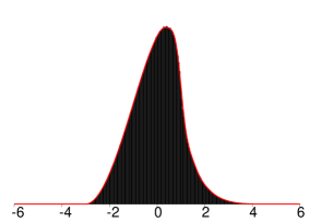
Figure 2. Trace distributions for Examples 5.4, 5.5, and 5.6

The red lines in Figure 2 show the densities of the theoretical trace distributions, as predicted by the Sato–Tate conjecture. For example 5.4, one has the superposition of the distributions for the two components, as explained in Section 3. Note that the theoretical density for Example 5.6 is not symmetric.

An example with CM by ${\mathbbm{Q}}(\sqrt{-1})$

Example 5.7.

Let $X_{4}^{\prime}$ be the double cover of ${\text{\bf P}}^{2}_{\mathbbm{Q}}$, given by

$$w^{2}=xyz(x+y+z)(x+2y+3z)(5x+8y+20z)$$

and $X_{4}$ the $K3$ surface obtained as the minimal desingularisation of $X_{4}^{\prime}$.

• Then the geometric Picard rank of $X_{4}$ is $16$.

• The endomorphism field of $X_{4}$ is $E={\mathbbm{Q}}(\sqrt{-1})$.

Proof. a) One has a lower bound of $16$, as the ramification locus has 15 singular points. An upper bound of $16$ is provided by the reduction modulo $13$, which is of geometric Picard rank $16$.

b) The reduction modulo $11$ is of geometric Picard rank $18$, which, as in Example 5.4, leaves $\smash{E={\mathbbm{Q}}(\sqrt{-1})}$ as the only nontrivial option. The result follows from Theorem A.1 below, as the endomorphism field does not shrink under specialisation [EJ20a, Corollary 4.6].   $\square$

Here, Corollary 4.9 yields $(\mathop{\text{\rm ST}}\nolimits^{2}(X_{4}))^{0}\cong\mathop{\text{\rm U}}\nolimits_{3}$. Moreover, for the component group, one has $\mathop{\text{\rm ST}}\nolimits^{2}_{\text{\rm tr}}(X_{4})/(\mathop{\text{\rm ST}}\nolimits^{2}(X_{1}))^{0}={\mathbbm{Z}}/2{\mathbbm{Z}}$. Indeed, (8) gives an upper bound of ${\mathbbm{Z}}/2{\mathbbm{Z}}$, and there must be a second component, due to the nontrivial jump character, cf. Table 6.

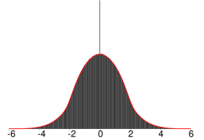
Figure 3. Trace distribution for Example 5.7

In the figure above, the spike is of mass $1/2$.

An example with RM and a cyclic component group of order four

Example 5.8.

Let $X_{5}^{\prime}$ be the double cover of ${\text{\bf P}}^{2}_{\mathbbm{Q}}$, given by

$$w^{2}=xy(x^{4}-7x^{3}y-x^{3}z+19x^{2}y^{2}+4x^{2}yz+x^{2}z^{2}-23xy^{3}-7xy^{2}z-6xyz^{2}$$

$${}-xz^{3}+11y^{4}+7y^{3}z+9y^{2}z^{2}+3yz^{3} +z^{4})$$

and $X_{5}$ the $K3$ surface obtained as the minimal desingularisation of $X_{5}^{\prime}$.

• Then the geometric Picard rank of $X_{5}$ is $16$.

• The endomorphism field of $X_{5}$ is $E={\mathbbm{Q}}(\sqrt{5})$.

Proof. a) One has a lower bound of $16$, as the ramification locus has 15 singular points. As far as upper bounds are concerned, the reductions modulo $7$ and $19$ are both of geometric Picard rank $18$. The characteristic polynomials of the Frobenii are

$$\textstyle(t-1)^{6}(t+1)^{4}(t^{2}+1)^{4}(t^{4}-\frac{12}{7}t^{2}+1)\quad{\rm and}\quad(t-1)^{10}(t+1)^{8}(t^{4}-\frac{4}{19}t^{3}+\frac{34}{19}t^{2}-\frac{4}{19}t+1)\,,$$

so that the Artin–Tate formula [Mi, Theorem 6.1] determines the discriminants of the four-dimensional lattices to $\overline{1}$ and $\overline{5}\in{\mathbbm{Q}}^{*}/{\mathbbm{Q}}^{*2}$, respectively. I.e., the lattices are incompatible and van Luijk’s method [vL] lets the upper bound drop to $17$.

On the other hand, the endomorphism field of $X_{5}$ contains $\smash{{\mathbbm{Q}}(\sqrt{5})}$, which excludes the option of rank $17$. Indeed, $X_{5}$ is isomorphic to the specialisation to $t=0$ of the family described in [EJ20a, Example 1.5]. The isomorphism is induced by the automorphism of ${\text{\bf P}}^{2}_{\overline{\mathbbm{Q}}}$, given by the matrix

$$\left(\begin{array}[]{rrr}1&\;2&\;0\\ 0&1&0\\ 0&0&1\end{array}\right)\,.\vskip 6.0pt plus 2.0pt minus 2.0pt$$

b) In view of a), this follows from [EJ20a, Example 1.5.iv)].   $\square$

Corollary 4.9 shows that $(\mathop{\text{\rm ST}}\nolimits^{2}(X_{5}))^{0}\cong[\mathop{\text{\rm SO}}\nolimits_{3}({\mathbbm{R}})]^{2}$.

Theorem 5.9.

The representation $\smash{\varrho^{2}_{X_{5},l,\text{\rm tr}}}$ induces an isomorphism

$$\overline{\varrho}\colon\mathop{\text{\rm Gal}}\nolimits({\mathbbm{Q}}(\zeta_{5})/{\mathbbm{Q}})\longrightarrow\mathop{\text{\rm ST}}\nolimits^{2}_{\text{\rm tr}}(X_{5})/(\mathop{\text{\rm ST}}\nolimits^{2}(X_{5}))^{0}\,.$$

Proof. First step. Generalities.

The jump character is trivial, so $\mathop{\text{\rm ST}}\nolimits^{2}_{\text{\rm tr}}(X_{5})/(\mathop{\text{\rm ST}}\nolimits^{2}(X_{5}))^{0}$ is bound to the cosets $\smash{\genfrac{(}{)}{0.0pt}{}{+\,\,0}{\,0\,\,+}}$, $\smash{\genfrac{(}{)}{0.0pt}{}{-\,\,0}{\,0\,\,-}}$, $\smash{\genfrac{(}{)}{0.0pt}{}{\,0\,\,+}{-\,\,0}}$, and $\smash{\genfrac{(}{)}{0.0pt}{}{\,0\,\,-}{+\,\,0}}$. Quite generally, there exists a unique number field $L_{0}$, for which $\smash{\varrho^{2}_{X_{5},l,\text{\rm tr}}}$ induces an isomorphism $\smash{\overline{\varrho}\colon\mathop{\text{\rm Gal}}\nolimits(L_{0}/{\mathbbm{Q}})\stackrel{{\scriptstyle\cong}}{{\longrightarrow}}\mathop{\text{\rm ST}}\nolimits^{2}_{\text{\rm tr}}(X_{5})/(\mathop{\text{\rm ST}}\nolimits^{2}(X_{5}))^{0}}$, cf. Remark 2.4.i). In our situation, we find that $\smash{L_{0}}$ is cyclic of a degree dividing four.

Second step. $\smash{L_{0}\supsetneqq{\mathbbm{Q}}(\sqrt{5})}$.

According to Chebotarev, the elements $\smash{\tau^{-1}\mathop{\text{\rm Frob}}\nolimits_{p}\tau}$, for $\smash{\tau\in\mathop{\text{\rm Gal}}\nolimits(\overline{\mathbbm{Q}}/{\mathbbm{Q}})}$ and $p\equiv 2,3\pmod{5}$, are dense in the nontrivial coset $\smash{C_{5}:=\mathop{\text{\rm Gal}}\nolimits(\overline{\mathbbm{Q}}/{\mathbbm{Q}})\setminus U_{5}}$ of the open subgroup $\smash{U_{5}:=\mathop{\text{\rm Gal}}\nolimits(\overline{\mathbbm{Q}}/{\mathbbm{Q}}(\sqrt{5}))\subset\mathop{\text{\rm Gal}}\nolimits(\overline{\mathbbm{Q}}/{\mathbbm{Q}})}$ of index two. Moreover, [EJ20a, Lemma 6.7] shows together with Lemma 4.5 that $\smash{\text{\rm Tr}(\varrho^{2}_{X_{5},l,\text{\rm tr}}(\mathop{\text{\rm Frob}}\nolimits_{p}))=0}$, for every prime $p\equiv 2,3\pmod{5}$. Consequently,

$$\text{\rm Tr}(\varrho^{2}_{X_{5},l,\text{\rm tr}}(\sigma))=0\,,$$ (9)

for every $\sigma\in C_{5}$.

Since, $\smash{U_{5}\subset\mathop{\text{\rm Gal}}\nolimits(\overline{\mathbbm{Q}}/{\mathbbm{Q}})}$ is a subgroup of finite index, $\smash{\overline{\varrho^{2}_{X_{5},l,\text{\rm tr}}(U_{5})}\subseteq G_{X_{5},l,\text{\rm tr}}^{2,\text{\rm Zar}}}$ has the same neutral component, only the component group may differ. Moreover, due to (9), $\smash{\overline{\varrho^{2}_{X_{5},l,\text{\rm tr}}(C_{5})}\subseteq G_{X_{5},l,\text{\rm tr}}^{2,\text{\rm Zar}}}$ is certainly a nontrivial coset. In particular, $\smash{\overline{\varrho^{2}_{X_{5},l,\text{\rm tr}}(U_{5})}}$ must be a proper subgroup of $\smash{G_{X_{5},l,\text{\rm tr}}^{2,\text{\rm Zar}}}$, which yields that $\smash{L_{0}\supseteq{\mathbbm{Q}}(\sqrt{5})}$.

Furthermore, (9) shows that the coset $\smash{\overline{\varrho^{2}_{X_{5},l,\text{\rm tr}}(C_{5})}}$ consists only of components of type $\smash{\genfrac{(}{)}{0.0pt}{}{\,0\,\,+}{-\,\,0}}$ and $\smash{\genfrac{(}{)}{0.0pt}{}{\,0\,\,-}{+\,\,0}}$. In particular, $\mathop{\text{\rm ST}}\nolimits^{2}_{\text{\rm tr}}(X_{5})/(\mathop{\text{\rm ST}}\nolimits^{2}(X_{5}))^{0}$ is indeed of order four.

Third step. Conclusion.

A standard argument involving the smooth specialisation theorem for étale cohomology groups [SGA4, Exp. XVI, Corollaire 2.2] shows that $L_{0}$ is unramified at every prime $p\neq 2$, $5$, and $l$, cf. [CEJ, Lemma 2.2.3.a)]. The field $L_{0}$ is, moreover, known to be independent of $l$ [Se81, p. 16, Théorème], cf. [Se12, §8.3.4]. Thus, working with $l=2$ or $5$, one finds that $L_{0}$ may ramify only at $2$ and $5$.

Besides $\smash{{\mathbbm{Q}}(\zeta_{5})}$, there are only three cyclic number fields of degree four that are unramified outside $2$ and $5$ and contain $\smash{{\mathbbm{Q}}(\sqrt{5})}$. These are the quadratic twists of $\smash{{\mathbbm{Q}}(\zeta_{5})}$ by $\smash{{\mathbbm{Q}}(\sqrt{\delta})}$, for $\delta=-1$, $2$, and $(-2)$. I.e., the unique further cyclic subfield of degree four in $\smash{{\mathbbm{Q}}(\zeta_{5},\sqrt{\delta})}$. Indeed, let $L$ be such a field. Then, since $\smash{\sqrt{5}\in L}$ and $\smash{\sqrt{5}\in{\mathbbm{Q}}(\zeta_{5})}$, the field $\smash{L(\zeta_{5})}$ has Galois group ${\mathbbm{Z}}/4{\mathbbm{Z}}\times{\mathbbm{Z}}/2{\mathbbm{Z}}$. Thus, $\smash{L(\zeta_{5})={\mathbbm{Q}}(\zeta_{5},\sqrt{\delta})}$, for some $\delta\in{\mathbbm{Z}}$. The claim follows, as $\smash{L(\zeta_{5})}$ is unramified outside $2$ and $5$.

Suppose that $L_{0}$ is the quadratic twist of $\smash{{\mathbbm{Q}}(\zeta_{5})}$ by $\smash{{\mathbbm{Q}}(\sqrt{\delta})}$, for $\delta=-1$, $2$, or $(-2)$. Then $\mathop{\text{\rm Frob}}\nolimits_{p}\in\mathop{\text{\rm Gal}}\nolimits(L_{0}/{\mathbbm{Q}})$ is not the neutral element for $p=11$ in the first two cases, and for $p=31$ in the third. However, an experiment shows that $\smash{\varrho^{2}_{X_{5},l,\text{\rm tr}}(\mathop{\text{\rm Frob}}\nolimits_{11})}$ and $\smash{\varrho^{2}_{X_{5},l,\text{\rm tr}}(\mathop{\text{\rm Frob}}\nolimits_{31})}$ are contained in the neutral component, which completes the proof.   $\square$

An example with RM and the Klein four group as the component group

Example 5.10.

Let $X_{6}^{\prime}$ be the double cover of ${\text{\bf P}}^{2}_{\mathbbm{Q}}$, given by

$$w^{2}=xyz(x^{3}-14x^{2}z+11xy^{2}-xz^{2}+12y^{3}-14y^{2}z-12yz^{2}+14z^{3})$$

and $X_{6}$ the $K3$ surface obtained as the minimal desingularisation of $X_{6}^{\prime}$.

• Then the geometric Picard rank of $X_{6}$ is $16$.

• The endomorphism field of $X_{6}$ is at most quadratic.

Proof. a) For the lower bound, the situation is analogous to [CEJ, Example 2.7.3]. One immediately has a lower bound of $13$, as the ramification locus has twelve singular points. Among them, ten are ${\mathbbm{Q}}$-rational, the two others are defined over $\smash{{\mathbbm{Q}}(\sqrt{-47})}$, and conjugate to each other. Moreover, there are a ${\mathbbm{Q}}$-rational line, the inverse image of which splits over $\smash{{\mathbbm{Q}}(\sqrt{14})}$, and two conics that are defined over $\smash{{\mathbbm{Q}}(\sqrt{-1})}$ and conjugate to each other, the inverse images of which split over $\smash{{\mathbbm{Q}}(\sqrt{-1},\sqrt{42})}$. Thus, there is a sublattice $\smash{P\subseteq\mathop{\text{\rm Pic}}\nolimits X_{6,\overline{\mathbbm{Q}}}}$ of rank $16$, such that $\smash{P\otimes_{\mathbbm{Z}}{\mathbbm{C}}=\chi_{\text{\rm triv}}^{12}\oplus\chi_{{\mathbbm{Q}}(\sqrt{-47})}\oplus\chi_{{\mathbbm{Q}}(\sqrt{14})}\oplus\chi_{{\mathbbm{Q}}(\sqrt{42})}\oplus\chi_{{\mathbbm{Q}}(\sqrt{-42})}}$ (cf. [CEJ] for notation). It is a routine work that was carried out with some help of the machine to set up an intersection matrix and to calculate that $\mathop{\text{\rm disc}}\nolimits(P\!\otimes_{\mathbbm{Z}}\!{\mathbbm{Q}})=(-3)\in{\mathbbm{Q}}^{*}/{\mathbbm{Q}}^{*}{}^{2}$.

Concerning an upper bound, the reductions modulo $19$ and $59$ are both of geometric Picard rank $18$. The characteristic polynomials of the Frobenii are

$$\textstyle(t-1)^{14}(t+1)^{4}(t^{4}+\frac{36}{19}t^{2}+1)\quad{\rm and}\quad(t-1)^{14}(t+1)^{4}(t^{4}-\frac{116}{59}t^{3}+\frac{162}{59}t^{2}-\frac{116}{59}t+1)\,,$$

so that the Artin–Tate formula [Mi, Theorem 6.1] determines the discriminants of the four-dimensional lattices to $\overline{1}$ and $\overline{6}\in{\mathbbm{Q}}^{*}/{\mathbbm{Q}}^{*2}$, respectively. I.e., the lattices are incompatible and van Luijk’s method [vL] lets the upper bound drop to $17$.

At this point, a modification of the method described in [EJ11] allows to reduce the upper bound even further. For this, suppose that one had $\smash{\mathop{\text{\rm rk}}\nolimits\mathop{\text{\rm Pic}}\nolimits X_{6,\overline{\mathbbm{Q}}}=17}$. The $\smash{\mathop{\text{\rm Gal}}\nolimits(\overline{\mathbbm{Q}}/{\mathbbm{Q}})}$-representation $\smash{\mathop{\text{\rm Pic}}\nolimits X_{6,\overline{\mathbbm{Q}}}\otimes_{\mathbbm{Z}}{\mathbbm{Q}}}$ then splits off a one-dimensional direct summand $\smash{V\subset(P\otimes_{\mathbbm{Z}}{\mathbbm{Q}})^{\perp}}$.

Let us particularly consider the action of $\smash{\mathop{\text{\rm Frob}}\nolimits_{19}\in\mathop{\text{\rm Gal}}\nolimits(\overline{\mathbbm{Q}}/{\mathbbm{Q}})}$. The characteristic polynomial on the whole of $\smash{\mathop{\text{\rm Pic}}\nolimits X_{6,\overline{\mathbbm{Q}}}\otimes_{\mathbbm{Z}}{\mathbbm{Q}}}$ is then $\smash{(t-1)^{14}(t+1)^{4}(t^{4}+\frac{36}{19}t^{2}+1)}$. Furthermore, as $(-47)$, $14$, $(-1)$, and $(-42)$ are all quadratic non-residues modulo $19$, the action splits $\smash{P\otimes_{\mathbbm{Z}}{\mathbbm{Q}}}$ into a $13$-dimensional invariant subspace $(P\otimes_{\mathbbm{Z}}{\mathbbm{Q}})^{+}$ and a three-dimensional $(-1)$-eigenspace $(P\!\otimes_{\mathbbm{Z}}\!{\mathbbm{Q}})^{-}$. Having set up in magma the corresponding intersection matrices with respect to suitable bases, one calculates that $\smash{\mathop{\text{\rm disc}}\nolimits((P\!\otimes_{\mathbbm{Z}}\!{\mathbbm{Q}})^{+})=\overline{2}\in{\mathbbm{Q}}^{*}/{\mathbbm{Q}}^{*}{}^{2}}$ and $\smash{\mathop{\text{\rm disc}}\nolimits((P\!\otimes_{\mathbbm{Z}}\!{\mathbbm{Q}})^{-})=(-\overline{6})\in{\mathbbm{Q}}^{*}/{\mathbbm{Q}}^{*}{}^{2}}$.

Moreover, the characteristic polynomial of $\mathop{\text{\rm Frob}}\nolimits_{19}$ on $\smash{(P\otimes_{\mathbbm{Z}}{\mathbbm{Q}})^{\perp}}$ turns out to be $\smash{(t-1)(t+1)(t^{4}+\frac{36}{19}t^{2}+1)}$. Therefore, $V$ may only be one of the one-dimensional eigenspaces, either $V^{+}_{19}$ or $V^{-}_{19}$. On the other hand, an application of the Artin–Tate formula shows that $\smash{\mathop{\text{\rm disc}}\nolimits((P\!\otimes_{\mathbbm{Z}}\!{\mathbbm{Q}})^{+}\!\!\perp\!V^{+}_{19})=(-\overline{74})\in{\mathbbm{Q}}^{*}/{\mathbbm{Q}}^{*}{}^{2}}$. I.e., that $\smash{\mathop{\text{\rm disc}}\nolimits(V^{+}_{19})=(-\overline{37})\in{\mathbbm{Q}}^{*}/{\mathbbm{Q}}^{*}{}^{2}}$. Finally, the Artin–Tate formula for ${\mathbbm{F}}_{\!19^{2}}$ yields $\smash{\mathop{\text{\rm disc}}\nolimits((P\!\otimes_{\mathbbm{Z}}\!{\mathbbm{Q}})\!\perp\!V^{+}_{19}\!\perp\!V^{-}_{19})=(-\overline{1})\in{\mathbbm{Q}}^{*}/{\mathbbm{Q}}^{*}{}^{2}}$, so that $\smash{\mathop{\text{\rm disc}}\nolimits(V^{-}_{19})=(-\overline{111})\in{\mathbbm{Q}}^{*}/{\mathbbm{Q}}^{*}{}^{2}}$ results. Consequently, $\smash{\mathop{\text{\rm disc}}\nolimits(V)=(-\overline{37})}$ or $\smash{(-\overline{111})\in{\mathbbm{Q}}^{*}/{\mathbbm{Q}}^{*}{}^{2}}$.

From this, a contradiction arises when one repeats the argument for a suitable second prime number. For example, the action of $\mathop{\text{\rm Frob}}\nolimits_{127}$ on $\smash{P\!\otimes_{\mathbbm{Z}}\!{\mathbbm{Q}}}$ has exactly the same invariant subspace $(P\!\otimes_{\mathbbm{Z}}\!{\mathbbm{Q}})^{+}$. Moreover, on $\smash{(P\!\otimes_{\mathbbm{Z}}\!{\mathbbm{Q}})^{\perp}}$, both the $(+1)$- and $(-1)$-eigenspaces are again of dimension one. A calculation completely analogous to the one above indicates that nothing but $\smash{\mathop{\text{\rm disc}}\nolimits(V)=(-\overline{229})}$ or $(-\overline{687})\in{\mathbbm{Q}}^{*}/{\mathbbm{Q}}^{*}{}^{2}$ may happen. This provides the desired contradiction and hence completes the proof of a).

b) As there are reductions of rank $18$, this is a consequence of [EJ20a, Lemma 6.2].   $\square$

There is strong evidence that the endomorphism field of $X_{6}$ is in fact $E={\mathbbm{Q}}(\sqrt{3})$. The evidence has been described in [EJ16, Section 5]. Note that $\smash{X_{6}=V^{(3)}_{1,2}}$ in the notation of [EJ16, Conjectures 5.2]. Thus, conjecturally, $(\mathop{\text{\rm ST}}\nolimits^{2}(X_{6}))^{0}\cong[\mathop{\text{\rm SO}}\nolimits_{3}({\mathbbm{R}})]^{2}$.

The observation that $\smash{\text{\rm Tr}(\varrho^{2}_{X_{6},l,\text{\rm tr}}(\mathop{\text{\rm Frob}}\nolimits_{p}))=0}$ for all primes $p=\pm 5\pmod{12}$ has meanwhile been extended to $p<10^{8}$. As these are exactly the primes, at which the jump character evaluates to $(-1)$, the component group $\mathop{\text{\rm ST}}\nolimits^{2}_{\text{\rm tr}}(X_{6})/(\mathop{\text{\rm ST}}\nolimits^{2}(X_{6}))^{0}$ is bound to the elements written symbolically as $\smash{\genfrac{(}{)}{0.0pt}{}{+\,\,0}{\,0\,\,+}}$, $\smash{\genfrac{(}{)}{0.0pt}{}{-\,\,0}{\,0\,\,-}}$, $\smash{\genfrac{(}{)}{0.0pt}{}{\,0\,\,+}{+\,\,0}}$, and $\smash{\genfrac{(}{)}{0.0pt}{}{\,0\,\,-}{-\,\,0}}$.

The component $\smash{\genfrac{(}{)}{0.0pt}{}{-\,\,0}{\,0\,\,-}}$ is indeed met, thus the component group is isomorphic to the Klein four group. According to our experiments, $\smash{\overline{x}_{p}\in[\mathop{\text{\rm O}}\nolimits_{3}^{-}({\mathbbm{R}})]^{2}}$ if and only if $p\equiv\pm 1\pmod{12}$ and $\smash{(\frac{-2\cdot 7\cdot 47}{p})=-1}$.

The trace distributions in the RM examples

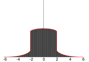
Figure 4. Trace distributions for Examples 5.8 and 5.10

In the figure above, each spike is of mass $1/2$. As before, the red lines show the densities of the theoretical trace distributions. They are obtained as the superpositions of the distributions for the two components $[\mathop{\text{\rm SO}}\nolimits_{3}({\mathbbm{R}})]^{2}$ and $[\mathop{\text{\rm O}}\nolimits_{3}^{-}({\mathbbm{R}})]^{2}$. The first is constructed as explained in Section 3, the second one by mirroring on the $y$-axis.

An example with CM by an endomorphism field of degree six

Example 5.11.

Let $X_{7}^{\prime}$ be the double cover of ${\text{\bf P}}^{2}_{\mathbbm{Q}}$, given by

$$w^{2}=xyz(x^{3}-3x^{2}z-3xy^{2}-3xyz+y^{3}+9y^{2}z+6yz^{2}+z^{3})$$

and $X_{7}$ the $K3$ surface obtained as the minimal desingularisation of $X_{7}^{\prime}$.

• Then the geometric Picard rank of $X_{7}$ is $16$.

• The endomorphism field of $X_{7}$ contains ${\mathbbm{Q}}(\sqrt{-1})$.

Proof. a) One has a lower bound of $16$, as the ramification locus has 15 singular points. An upper bound of $16$ is provided by the reduction modulo $5$, which is of geometric Picard rank $16$.

b) The automorphism of ${\text{\bf P}}^{2}_{\overline{\mathbbm{Q}}}$, given by the matrix

$$\left(\begin{array}[]{rrr}-g\!+\!1&g^{2}\!+\!g\!-\!1&g^{2}\\ 0&0&-g\\ 1&1&1\end{array}\right)\,,$$

for $g:=\zeta_{9}+\zeta_{9}^{-1}-1$, transforms $X_{7}$ into a fibre of the family $q\colon{\mathscr{X}}\to B$, considered in Theorem A.1. The assertion follows, as the endomorphism field does not shrink under specialisation.   $\square$

There is strong evidence that $X_{7}$ has complex multiplication by the endomorphism field $E={\mathbbm{Q}}(\zeta_{9}+\zeta_{9}^{-1},\sqrt{-1})$, which is abelian of degree six. The evidence has been described in [EJ16, last subsection]. Note that $\smash{X_{7}=V^{(-1,\mu_{9})}}$ in the notation of [EJ16, Conjectures 5.2]. Thus, conjecturally, $\smash{(\mathop{\text{\rm ST}}\nolimits^{2}(X_{7}))^{0}\cong[\mathop{\text{\rm U}}\nolimits_{1}]^{3}}$.

The observation that $\smash{\text{\rm Tr}(\varrho^{2}_{X_{7},l,\text{\rm tr}}(\mathop{\text{\rm Frob}}\nolimits_{p}))=0}$ for all primes $p\not\equiv\pm 1\pmod{36}$ has meanwhile been extended to $p<10^{8}$. If one knew this unconditionally then Example 4.13.b) would show that $\mathop{\text{\rm ST}}\nolimits^{2}_{\text{\rm tr}}(X_{7})/(\mathop{\text{\rm ST}}\nolimits^{2}(X_{7}))^{0}\cong{\mathbbm{Z}}/6{\mathbbm{Z}}$. Note that the maximal totally real subfield $E_{0}={\mathbbm{Q}}(\zeta_{9}+\zeta_{9}^{-1})$ of the conjectural endomorphism field is cyclic of degree $3$.

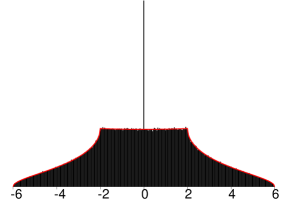
Figure 5. Trace distribution for Example 5.11

In the figure above, the spike is of mass $5/6$.

Conclusion

For each of the seven $K3$ surfaces in the sample, we see a strong coincidence in the data that supports the Sato–Tate conjecture.

The order of convergence

In Example 5.11, up to $10^{8}$, exactly $960\,272$ of the $5\,761\,455$ primes do not contribute to the spike. Only these are to be considered. Then, among the 300 subintervals, the largest discrepancy between the experimental count of Frobenius traces and the theoretical prediction occurs in the subinterval ranging from $1.72$ to $1.76$. Here, $5538.39$ Frobenius traces are to be expected, but only $5341$ are found, a relative error of roughly $3.5\%$.

$N:=$	Largest	Maximal #	Largest
#primes	discrepancy	of traces	discrepancy
		expected	$/\sqrt{\text{\#expected}}$
$32$	$\phantom{-00}1.918$	$\phantom{000}0.19$	$\phantom{-}4.46$
$64$	$\phantom{-00}1.836$	$\phantom{000}0.37$	$\phantom{-}3.02$
$128$	$\phantom{-00}3.261$	$\phantom{000}0.74$	$\phantom{-}3.79$
$256$	$\phantom{-00}3.804$	$\phantom{000}1.48$	$\phantom{-}3.13$
$512$	$\phantom{-00}5.092$	$\phantom{000}2.96$	$\phantom{-}2.96$
$1\,024$	$\phantom{-00}6.156$	$\phantom{000}5.93$	$\phantom{-}2.53$
$2\,048$	$\phantom{-00}9.285$	$\phantom{00}11.85$	$\phantom{-}2.70$
$4\,096$	$\phantom{-0}14.364$	$\phantom{00}23.70$	$\phantom{-}2.95$
$8\,192$	$\phantom{-0}23.728$	$\phantom{00}47.40$	$\phantom{-}3.44$
$16\,384$	$\phantom{-0}30.457$	$\phantom{00}94.80$	$\phantom{-}3.13$
$32\,768$	$\phantom{-0}41.965$	$\phantom{0}189.60$	$\phantom{-}3.05$
$65\,536$	$\phantom{-0}53.930$	$\phantom{0}379.21$	$\phantom{-}2.77$
$131\,072$	$\phantom{-0}75.102$	$\phantom{0}758.42$	$\phantom{-}2.73$
$262\,144$	$-129.287$	$1516.84$	$-3.32$
$524\,288$	$-146.727$	$3033.68$	$-2.66$
$960\,272$	$-197.392$	$5556.40$	$-2.65$

Table 4. Discrepancies between numbers of Frobenius traces

The maximal number of traces to be expected in a subinterval is $5556.40$. This number does not occur near $0.00$, but for the subintervals $[-2.00,-1.96]$ and $[1.96,2.00]$. One calculates that $(5341-5538.39)/\sqrt{5556.40}\approx-2.65$.

Doing the same for only the first $2^{k}$ good primes, not contributing to the spike, for $k=3,\ldots,19$, the data were obtained that are presented in Table 4 above. It seems that the values in the column to the right remain within a bounded range around zero.

As the maximal number of traces expected among the subintervals is proportional to the number of primes $N$, this suggests that the largest discrepancy is proportional to $\sqrt{N}$. Consequently, the $L^{0}$-distance between the experimental and theoretical density functions is proportional to $\smash{\frac{1}{\sqrt{N}}}$, which means that convergence is of order $\smash{\frac{1}{2}}$.

The order of convergence–A second experiment

Experts in Statistics advise to consider the $L^{0}$-distance between the experimental and theoretical distribution functions, instead of the densities. Again, the values in the column to the right seem to fluctuate within a bounded range around zero. Which would indeed show convergence of order $\smash{\frac{1}{2}}$.

	$L^{0}$-distance
$N:=$	between	multiplied
#primes	distribution	by $\sqrt{N}$
	functions
$8$	$-0.175$	$-0.496$
$16$	$-0.262$	$-1.049$
$32$	$-0.155$	$-0.877$
$64$	$-0.077\,5$	$-0.620$
$128$	$-0.047\,2$	$-0.534$
$256$	$\phantom{-}0.057\,2$	$\phantom{-}0.916$
$512$	$\phantom{-}0.034\,1$	$\phantom{-}0.772$
$1\,024$	$-0.018\,8$	$-0.601$
$2\,048$	$-0.013\,1$	$-0.595$
$4\,096$	$-0.007\,40$	$-0.473$
$8\,192$	$-0.007\,05$	$-0.638$
$16\,384$	$\phantom{-}0.004\,12$	$\phantom{-}0.527$
$32\,768$	$-0.003\,55$	$-0.642$
$65\,536$	$\phantom{-}0.003\,06$	$\phantom{-}0.783$
$131\,072$	$\phantom{-}0.001\,70$	$\phantom{-}0.615$
$262\,144$	$-0.001\,50$	$-0.770$
$524\,288$	$-0.001\,21$	$-0.874$
$960\,272$	$-0.000\,521$	$-0.511$

Table 5. $L^{0}$-distance between experimental and theoretical distribution functions

For the other six example surfaces, we made the analogous experiments. We do not think that it is useful to present the corresponding raw data in this article. In fact, all the surfaces examined show qualitatively the same behaviour.

The Lang–Trotter conjecture

Concerning the traces of the Frobenii $\mathop{\text{\rm Frob}}\nolimits_{p}$ on $\smash{H^{2}_{\text{\rm\'{e}t}}(X_{7,\overline{\mathbbm{Q}}},{\mathbbm{Q}}_{l})}$, the statistics for $p<10^{8}$ is as follows. There are $922\,644$ distinct integers occurring as a trace. One of them is $0$, which comes up roughly $\smash{\frac{5}{6}}$ of the time. Except for this, there are $886\,932$ integers that occur only once, $33\,922$ integers that occur exactly twice, $1\,667$ integers that occur exactly three times, $115$ integers that occur exactly four times, and $7$ integers that occur exactly five times as a trace. No integer occurs more than five times. Comparing this with $\log\log 10^{8}\approx 2.913$, there is certainly no contradiction with the Lang–Trotter conjecture to be seen from our data. Once again, the other examples show qualitatively the same behaviour.

Appendix A A family that is acted upon by ${\mathbbm{Q}}(\sqrt{-1})$

Theorem A.1.

Let $B\subset{\text{\bf P}}^{2}_{\mathbbm{Q}}\!\times\!{\text{\bf P}}^{2}_{\mathbbm{Q}}$ be the closed subscheme given by the equations $a_{1}b_{3}+a_{2}b_{1}-2a_{3}b_{1}=0$ and $a_{1}b_{2}+a_{2}b_{3}-2a_{3}b_{2}=0$, and let, moreover, $q\colon{\mathscr{X}}^{\prime}\to B$ be the family of double covers of ${\text{\bf P}}^{2}$ given by

$$w^{2}=l_{1}\cdots l_{6}\,,$$

for $l_{1},\ldots,l_{6}$ the linear forms $l_{1}:=x$, $l_{2}:=y$, $l_{3}:=z$, $l_{4}:=x+y+z$, $l_{5}:=a_{1}x+a_{2}y+a_{3}z$, and $l_{6}:=b_{1}x+b_{2}y+b_{3}z$.

• Then the generic fibre ${\mathscr{X}}^{\prime}_{\eta}$ is normal surface, the minimal desingularisation of which is a $K3$ surface ${\mathscr{X}}_{\eta}$ of geometric Picard rank $16$.

• The endomorphism field of ${\mathscr{X}}_{\eta}$ is ${\mathbbm{Q}}(\sqrt{-1})$.

Proof. a) The singularities of ${\mathscr{X}}^{\prime}_{\eta}$ are caused by those of the ramification curve, and are therefore isolated and of type $A_{1}$. The surface ${\mathscr{X}}_{\eta}$ is a $K3$ surface as the ramification curve is of degree six. For the geometric Picard rank, one has a lower bound of $16$, as the ramification locus has 15 singular points. An upper bound of $16$ is provided by the specialisation to $X_{4}$, cf. Example 5.7.c).

b) The specialisation to $X_{4}$ is known to have an endomorphism field of degree $\leq\!2$, cf. Example 5.7.d). As the endomorphism field does not shrink under specialisation [EJ20a, Corollary 4.6], it is sufficient to show that the endomorphism field of $\smash{{\mathscr{X}}_{\eta}}$ contains $\smash{{\mathbbm{Q}}(\sqrt{-1})}$.

For this, we blow up $\smash{{\text{\bf P}}^{2}_{k(B)}}$ in the seven points ${\text{\bf V}}(l_{i},l_{j})$, for $\{i,j\}=\{1,2\}$, $\{1,4\}$, $\{1,6\}$, $\{2,4\}$, $\{2,6\}$, $\{4,6\}$, and $\{3,5\}$. Since no four of these points are collinear, the result is a weak del Pezzo surface $S$ of degree $2$ [Do, Corollary 8.1.24]. The linear system of the cubic forms vanishing in the seven blown-up points defines a birational morphism $S\to S^{\prime}$ to a singular model $S^{\prime}\colon W^{2}=Q(X,Y,Z)$. Here, $Q$ defines a plane quartic having only simple singularities [Do, Theorem 8.3.2.(iv)]. A calculation shows that, in our particular situation, the quartic ${\text{\bf V}}(Q)$ splits over $k(B)$ into the union of two conics, $Q=Q_{1}Q_{2}$.

The double cover $\smash{{\mathscr{X}}^{\prime}_{\eta}}$ of $\smash{{\text{\bf P}}^{2}_{k(B)}}$ goes over, under blowing up, into a double cover of $S$, and therefore also into one of $S^{\prime}$. The special choice of $B$ makes sure that the ramification locus ${\text{\bf V}}(l_{1}\cdots l_{6})$ is mapped to ${\text{\bf V}}(Q)$. In other words, a linear algebra calculation over the function field $k(B)$ shows that three linearly independent cubic forms vanishing in the seven blown-up points, together with the coordinate $w$, fulfil exactly one quartic relation, which is of the kind $W^{4}=Q(X,Y,Z)$. I.e., ${\mathscr{X}}_{\eta}$ has a singular model ${\mathscr{X}}^{\prime\prime}_{\eta}$ of degree four, which is given by the equation

$$W^{4}=Q_{1}(X,Y,Z)Q_{2}(X,Y,Z)\,.$$

There is an automorphism of ${\mathscr{X}}^{\prime\prime}_{\eta}$, given by $I\colon(W\!:\!X\!:\!Y\!:\!Z)\mapsto(iW\!:\!X\!:\!Y\!:\!Z)$, cf. [EJ20b, Example 6.17]. We claim that the operation of $I$ on $H_{\text{\rm tr}}$ gives rise to complex multiplication. For this, it has to be shown that $J:=I\!\circ\!I$ acts on $H_{\text{\rm tr}}$ as the multiplication by $(-1)$. Let us note that $H_{\text{\rm tr}}$ is a simple ${\mathbbm{Q}}$-Hodge structure [Za, Theorem 1.6.a)], so it suffices to exclude multiplication by $(+1)$.

For this, observe that $\smash{{\mathscr{X}}^{\prime\prime}_{\eta}}$ has four singularities, each of which is of type $A_{3}$. Hence, $\smash{\dim H^{2}({\mathscr{X}}^{\prime\prime}_{\eta}({\mathbbm{C}}),{\mathbbm{Q}})=10}$. The fixed point set of $J$ is the union of two conics, which has topological Euler characteristic $0$. Therefore, the Lefschetz trace formula [Ed, Theorem 8.5] shows that $\smash{\text{\rm Tr}(J|_{H^{2}({\mathscr{X}}^{\prime\prime}_{\eta}({\mathbbm{C}}),{\mathbbm{Q}})})=-2}$. In other words, $\smash{J|_{H^{2}({\mathscr{X}}^{\prime\prime}_{\eta}({\mathbbm{C}}),{\mathbbm{Q}})}}$ has the eigenvalue $(+1)$ with multiplicity $4$, while the eigenvalue $(-1)$ occurs with multiplicity $6$. In particular, $\smash{H_{\text{\rm tr}}}$, which is of dimension six, cannot be contained in the $(+1)$-eigenspace, which completes the proof.   $\square$

Appendix B A table

$i$	1	2	3	4	5	6	7
Bad primes of $X_{i}$	$2,3,5,7,$	$2,3,5,7$	$2,3,5$	$2,3,5,$	$2,5$	$2,3,5,7,$	$2,3$
	$11,13,29$			$7,11$		$11,13,17,47$
Jump character
$\Delta_{\text{\rm tr}}\in{\mathbbm{Q}}^{*}/{\mathbbm{Q}}^{*2}$ of $X_{i}$	$-\overline{6006}$	$\overline{1}$	$\overline{1}$	$-\overline{1}$	$\overline{1}$	$(\overline{3})$	$-\overline{1}$

Table 6. Bad primes and jump character for the surfaces in the sample

References

- [BHPV] Barth, W., Hulek, K., Peters, C., and Van de Ven, A.: Compact complex surfaces, Second edition, Ergebnisse der Mathematik und ihrer Grenzgebiete 4, Springer, Berlin 2004
- [Bo] Borel, A.: Linear algebraic groups, Second edition, Graduate Texts in Mathematics 126, Springer, New York 1991
- [BCP] Bosma, W., Cannon, J., and Playoust, C.: The Magma algebra system I. The user language, J. Symbolic Comput. 24 (1997), 235–265
- [Ch14] Charles, F.: On the Picard number of surfaces over number fields, Algebra Number Theory 8 (2014), 1–17
- [CHT] Clozel, L., Harris, M., and Taylor, R.: Automorphy for some -adic lifts of automorphic mod Galois representations, Publ. Math. IHES 108 (2008), 1–181
- [CEJ] Costa, E., Elsenhans, A.-S., and Jahnel, J.: On the distribution of the Picard ranks of the reductions of a surface, Research in Number Theory 6 (2020), art. 27, 25pp.
- [CT] Costa, E. and Tschinkel, Yu.: Variation of Néron-Severi ranks of reductions of surfaces, Exp. Math. 23 (2014), 475–481
- [De71] Deligne, P.: Théorie de Hodge II, Publ. Math. IHES 40 (1971), 5–57
- [De74] Deligne, P.: La conjecture de Weil I, Publ. Math. IHES 43 (1974), 273–307
- [De80] Deligne, P.: La conjecture de Weil II, Publ. Math. IHES 52 (1980), 137–252
- [De81] Deligne, P.: Relèvement des surfaces en caractéristique nulle (rédigé par L. Illusie), in: Surfaces algébriques (Orsay, 1976–78), Lecture Notes in Math. 868, Springer, Berlin-New York 1981, 58–79
- [Di] Dieudonné, J.: Éléments d’analyse. Tome II, Gauthier-Villars, Cahiers Scientifiques, Fasc. XXXI, Paris 1968
- [Do] Dolgachev, I. V.: Classical Algebraic Geometry: a modern view, Cambridge University press, Cambridge 2012
- [Ed] Edmonds A. L.: Introduction to transformation groups, www.indiana.edu/~jfdavis/seminar/transformationgroupsb.pdf
- [EJ11] Elsenhans, A.-S. and Jahnel, J.: On the computation of the Picard group for surfaces, Mathematical Proceedings of the Cambridge Philosophical Society 151 (2011), 263–270
- [EJ14] Elsenhans, A.-S. and Jahnel, J.: Examples of surfaces with real multiplication, in: Proceedings of the ANTS XI conference (Gyeongju 2014), LMS Journal of Computation and Mathematics 17 (2014), 14–35
- [EJ16] Elsenhans, A.-S. and Jahnel, J.: Point counting on surfaces and an application concerning real and complex multiplication, in: Algorithmic number theory (Kaiserslautern 2016), LMS Journal of Computation and Mathematics 19 (2016), 12–28
- [EJ20a] Elsenhans, A.-S. and Jahnel, J.: Explicit families of K3 surfaces having real multiplication, To appear in: Michigan Mathematical Journal
- [EJ20b] Elsenhans, A.-S. and Jahnel, J.: Real and complex multiplication on K3 surfaces via period integration, To appear in: Experimental Mathematics
- [EJ22] Elsenhans, A.-S. and Jahnel, J.: -adic point counting on surfaces, https://arxiv.org/abs/2202.10853
- [EP] Evans, D. E. and Pugh, M.: Spectral measures associated to rank two Lie groups and finite subgroups of , Comm. Math. Phys. 343 (2016), 811–850
- [FKRS] Fité, F., Kedlaya, K., Rotger, V., and Sutherland, A.: Sato-Tate distributions and Galois endomorphism modules in genus , Compos. Math. 148 (2012), 1390–1442
- [FS] Fité, F. and Sutherland, A.: Sato–Tate distributions of twists of and , Algebra & Number Theory 8 (2014), 543–585
- [vG] van Geemen, B.: Real multiplication on surfaces and Kuga-Satake varieties, Michigan Math. J. 56 (2008), 375–399
- [HST] Harris, M., Shepherd-Barron, N., and Taylor, R.: A family of Calabi-Yau varieties and potential automorphy, Ann. of Math. 171 (2010), 779–813
- [Ha] Harvey, D.: Computing zeta functions of arithmetic schemes, Proc. Lond. Math. Soc. 111 (2015), 1379–1401
- [Jo] Joyce, G. S.: On the simple cubic lattice Green function, Philos. Trans. Roy. Soc. London 273 (1973), 583–610
- [KS] Kedlaya, K. S. and Sutherland, A. V.: Hyperelliptic curves, L-polynomials, and random matrices, in: Arithmetic, geometry, cryptography and coding theory, Contemp. Math. 487, AMS, Providence 2009, 119–162
- [KM] Kendall, M. G. and Moran, P. A. P.: Geometrical probability, Griffin’s Statistical Monographs & Courses 10, Hafner Publishing Co., New York 1963
- [Kn] Knapp, A. W.: Lie groups beyond an introduction, Second edition, Progress in Mathematics 140, Birkhäuser, Boston 2002
- [La] Lachaud, G.: On the distribution of the trace in the unitary symplectic group and the distribution of Frobenius, in: Frobenius distributions: Lang-Trotter and Sato-Tate conjectures, Contemp. Math. 663, AMS, Providence 2016, 185–221
- [LT] Lang, S. and Trotter, H.: Frobenius distributions in -extensions, in: Distribution of Frobenius automorphisms in -extensions of the rational numbers, Lecture Notes in Mathematics 504, Springer, Berlin-New York 1976
- [Le] Lee, D. H.: The structure of complex Lie groups, Chapman & Hall/CRC Research Notes in Mathematics 429, CRC Press, Boca Raton 2002
- [vL] van Luijk, R.: surfaces with Picard number one and infinitely many rational points, Algebra & Number Theory 1 (2007), 1–15
- [Ma] Maplesoft, a division of Waterloo Maple Inc.: maple, Waterloo, Ontario 2019
- [Me] Meckes, E. S.: The random matrix theory of the classical compact groups, Cambridge Tracts in Mathematics 218, Cambridge University Press, Cambridge 2019
- [Mi] Milne, J. S.: On a conjecture of Artin and Tate, Ann. of Math. 102 (1975), 517–533
- [OV] Onishchik, A. L. and Vinberg, E. B. (eds.): Lie groups and Lie algebras III, Structure of Lie groups and Lie algebras, Springer, Berlin 1994
- [OEIS] Sloane, N. J. A. (ed.): The On-Line Encyclopedia of Integer Sequences, published electronically at https://oeis.org
- [Se68] Serre, J.-P.: Abelian -adic representations and elliptic curves, W. A. Benjamin Inc., New York-Amsterdam 1968
- [Se70] Serre, J.-P.: Cours d’arithmétique, Presses Universitaires de France, Paris 1970
- [Se72] Serre, J.-P.: Propriétés galoisiennes des points d’ordre fini des courbes elliptiques, Invent. Math. 15 (1972), 259–331
- [Se81] Serre, J.-P.: Lettres à Ken Ribet du 1/1/1981 et du 29/1/1981, in: Oeuvres–Collected Papers, Volume IV, Springer, Berlin 2000, 1–20
- [Se12] Serre, J.-P.: Lectures on , Chapman & Hall/CRC Research Notes in Mathematics 11, CRC Press, Boca Raton 2012
- [SGA4] Artin, M., Grothendieck, A. et Verdier, J.-L. (avec la collaboration de Deligne, P. et Saint-Donat, B.): Théorie des topos et cohomologie étale des schémas, Séminaire de Géométrie Algébrique du Bois Marie 1963–1964 (SGA 4), Lecture Notes in Math. 269, 270, 305, Springer, Berlin, Heidelberg, New York 1972–1973
- [SGA5] Grothendieck, A. (avec la collaboration de Bucur, I., Houzel, C., Illusie, L. et Serre, J.-P.): Cohomologie -adique et Fonctions , Séminaire de Géométrie Algébrique du Bois Marie 1965–1966 (SGA 5), Lecture Notes in Math. 589, Springer, Berlin, Heidelberg, New York 1977
- [Su19] Sutherland, A. V.: Sato-Tate distributions, in: Analytic methods in arithmetic geometry, Contemp. Math. 740, AMS, Providence 2019, 197–248
- [Su20] Sutherland, A. V.: https://math.mit.edu/drew/, Retrieved on December 1, 2020
- [Tan90] Tankeev, S. G.: Surfaces of type over number fields and the Mumford–Tate conjecture (Russian), Izv. Akad. Nauk SSSR Ser. Mat. 54 (1990), 846–861
- [Tan95] Tankeev, S. G.: Surfaces of type over number fields and the Mumford–Tate conjecture II (Russian), Izv. Ross. Akad. Nauk Ser. Mat. 59 (1995), 179–206
- [Tat] Tate, J.: Algebraic cycles and poles of zeta functions, in: Arithmetical Algebraic Geometry, Proc. Conf. Purdue Univ. 1963, Harper & Row, New York 1965, 93–110
- [Tay] Taylor, R.: Automorphy for some -adic lifts of automorphic mod Galois representations II, Publ. Math. IHES 108 (2008), 183–239
- [We] Wendt, R.: Weyl’s character formula for non-connected Lie groups and orbital theory for twisted affine Lie algebras, J. Funct. Anal. 180 (2001), 31–65
- [Wi] Wiles, A.: Modular elliptic curves and Fermat’s last theorem, Ann. of Math. 141 (1995), 443–551
- [Za] Zarhin, Yu. G.: Hodge groups of surfaces, J. Reine Angew. Math. 341 (1983), 193–220