Constraints on the latitudinal profile of Jupiter’s deep jets

Abstract

The observed zonal winds at Jupiter’s cloud tops have been shown to be closely linked to the asymmetric part of the planet’s measured gravity field. However, other measurements suggest that in some latitudinal regions the flow below the clouds might be somewhat different from the observed cloud-level winds. Here we show, using both the symmetric and asymmetric parts of the measured gravity field, that the observed cloud-level wind profile between 25^∘S and 25^∘N must extend unaltered to depths of thousands of kilometers. Poleward, the midlatitude deep jets also contribute to the gravity signal, but might differ somewhat from the cloud-level winds. We analyze the likelihood of this difference and give bounds to its strength. We also find that to match the gravity measurements, the winds must project inward in the direction parallel to Jupiter’s spin axis, and that their decay inward should be in the radial direction.

¹Department of Earth and Planetary Sciences, Weizmann Institute of Science, Rehovot, Israel.
²School of Physics and Astronomy, University of Leicester, Leicester, UK
³California Institute of Technology, Pasadena, CA, USA
⁴Department of Climate and Space Sciences and Engineering, University of Michigan, Ann Arbor, MI, USA
⁵Jet Propulsion Laboratory, California Institute of Technology, Pasadena, USA
⁶Observatoire de la Cote d’Azur, Nice, France
⁷Southwest Research Institute, San Antonio, Texas, TX, USA

1 Introduction

The zonal (east-west) wind at Jupiter’s cloud level dominate the atmospheric circulation, and strongly relate to the observed cloud bands Fletcher et al. (2020). The structure of the flow beneath the cloud level has been investigated by several of the instruments on board the Juno spacecraft by means of gravity, infrared and microwave measurements Bolton et al. (2017). Particularly, the gravity measurements were used to infer that the winds extend down to roughly 3000 km, and that the main north-south asymmetry in the cloud-level wind extends to these great depths Kaspi et al. (2018), resulting in the substantial values of the odd gravity harmonics $J_{3}$, $J_{5}$, $J_{7}$, and $J_{9}$. The excellent match between the sign and value of the predicted odd harmonics using the cloud-level wind Kaspi (2013) and the Juno gravity measurements Iess et al. (2018), led to the inference that the wind profile at depth is similar to that at the cloud level Kaspi et al. (2018, 2020). Here, we revisit in more detail the relation between the exact meridional profile of the zonal flow and the gravity measurements, and study how much of the cloud-level wind must be retained in order to match the gravity measurements.

Since the gravity measurements are sensitive to mass distribution, they are not very sensitive to the shallow levels (0.5-240 bar) probed by Juno’s microwave radiometer (MWR, Janssen et al., 2017), as the density in this region is low compared to the deeper levels. Yet, the gravity measurements have substantial implications on the MWR region, since if the flow profile at depth (below the MWR region) resembles that at the cloud level it is likely that the flow profile within the MWR region is not very different. In such a case, where the flow is barotropic, this implies via thermal wind balance that latitudinal temperature gradients in the MWR region are small, which has important implication to the MWR analysis of water and ammonia distribution Li et al. (2017); Ingersoll et al. (2017); Li et al. (2020). Thus, it is important to determine how strong the gravity constraint on the temperature distribution is, and what is its latitudinal dependence.

The determination of the zonal flow field at depth is based on the measurements of the odd gravity harmonics, $J_{3}$, $J_{5}$, $J_{7}$, and $J_{9}$, which are uniquely related to the flow field Kaspi (2013). Using only four numbers to determine a 2D (latitude and depth) field poses a uniqueness challenge, and solutions that are unrelated to the observed cloud-level wind can be found Kong et al. (2018), although the origin of such internal flow structure, completely unrelated to the cloud-level winds, is not clear. In addition, these solutions require a flow of about 1 m s^-1 at depth of 0.8 the radius of Jupiter ($\sim$15,000 km), where the significant conductivity Liu et al. (2008); Wicht et al. (2019) is expected to dampen such strong flows Cao and Stevenson (2017); Duer et al. (2019); Moore et al. (2019). Recently, (Galanti and Kaspi, 2021) showed that the interaction of the flow with the magnetic field in the semiconducting region can be used as an additional constraint on the structure of the flow below the cloud level. With some modification of the observed cloud-level wind, well within its uncertainty range Tollefson et al. (2017), a solution can be found that explains the odd gravity harmonics and abides the magnetic field constraints.

All of the above mentioned studies assumed that if the internal flow is related to the observed surface winds, it will manifest its entire latitudinal profile. However, some evidence suggests that at some latitudinal regions the flow below the clouds might be different from the winds at the cloud level. The Galileo probe, entering the Jovian atmosphere around planetocentric latitude 6.5^∘N Orton et al. (1998), measured winds that strengthened from 80 ms^-1 at the cloud level to $\sim$160 ms^-1 at a depth of 4 bars, from where it remains approximately constant until a depth of 20 bars where the probe stopped transmitting data Atkinson et al. (1998). Such a baroclinic shear got further support in studies of equatorial hot spots Li et al. (2006); Choi et al. (2013). Recently, Duer et al. (2020) showed that the MWR measurements of brightness temperature correlate to the zonal wind’s latitudinal profile. They found that profiles differing to a limited extent from the cloud-level can still be consistent with both MWR and gravity. Emanating from the correlations between MWR and the zonal winds, Fletcher et al. (2021) suggested that the winds at some latitudes might strengthen from the cloud level to a depth of 4-8 bars, i.e. not far from where water is expected to be condensing, and only then begin to decay downward. Alternatively, based on stability considerations, it was suggested that while westward jets are not altered much with depth, the eastward jets might increase by 50-100% Dowling (1995, 2020).

Furthermore, in the Kaspi et al. (2018) and Galanti and Kaspi (2021) studies, the observed cloud-level wind has been assumed to be projected into the planet interior along the direction parallel to the spin axis of Jupiter, based on theoretical arguments (Busse, 1970, 1976) and 3D simulations of the flow in a Jovian-like planet (e.g., Busse, 1994; Kaspi et al., 2009; Christensen, 2001; Heimpel et al., 2016). Theoretically this requires the flow to be nearly barotropic, which is not necessarily the case, particularly when considering the 3D nature of the planetary interior. Another assumption made is that the flow decays in the radial direction. This was based on the reasoning that any mechanism acting to decay the flow, such as the increasing conductivity (Cao and Stevenson, 2017), compressibility (Kaspi et al., 2009), or the existence of a stable layer (Debras and Chabrier, 2019; Christensen et al., 2020), will depend on pressure and temperature, which to first order are a function of depth. However, if the internal flow is organized in cylinders it might be the case that the mechanism acting to decay it strengthens also in the direction parallel to the spin axis.

Here we investigate what can be learned about the issues discussed above, based on the measured gravity field, considering both the symmetric and asymmetric components of the gravity field measurements. We study the ability to fit the gravity measurements with a cloud-level wind that is limited to a specific latitudinal range, thus identifying the regions where the observed cloud-level wind is likely to extend deep, and the regions where the interior flow might differ (section 3). We also examine whether a stronger wind at the 4-8 bar level is compatible with the gravity measurements, and if the assumptions regarding the relation of the internal flow to the cloud level can be relaxed (section 4). Finally, we examine the latitudinal dependence of the wind-induced gravity harmonics when magnetohydrodynamics considerations are used as additional constraints (section 5).

2 Defining the cloud-level wind and possible internal flow structures

We examine several aspects of the flow structure that might influence the ability to explain the gravity measurements. First, stemming from the notion that at some latitudinal regions the flow below the cloud level might differ from the observed, we set cases in which the cloud-level wind is truncated at a specific latitude (Fig. 1a). The truncation is done by applying a shifted hemispherically symmetric hyperbolic tangent function with a transition width of 5^∘, to allow a smooth truncation of the wind from the observed flow. The result is a wind profile that equatorward of the truncation latitude is kept as in the cloud-top observations, and poleward decays quickly to zero. We examine 18 cases with truncation latitudes $5^{\circ},10^{\circ},15^{\circ},...,90^{\circ}$. Note that all of the cloud-level wind setups used in this study are based on the analysis of the HST Jupiter images during Juno’s PJ3 (Tollefson et al., 2017)[, Figure 1a, gray line], and that in all figures and calculations we use the planetocentric latitude.

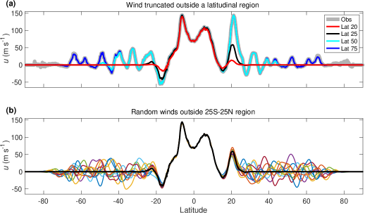
Figure 1: (a) The observed wind (Tollefson et al., 2017) (gray), and variant examples with the wind truncated poleward of the latitudes 20^∘, 25^∘, 50^∘, and 75^∘. (b) The case of wind truncated poleward of the 25^∘ latitude (black), along with examples of random jets added in the truncated regions.

Next, we examine cases in which a different wind structure exists poleward of the truncation latitude. As such, unknown wind structures could possibly replace the observed cloud-level wind at shallow depths of around 5-10 bars (e.g., as can be inferred from MWR, depending on how microwave brightness temperatures are interpreted, see Fletcher et al. 2021). For the purpose of the gravity calculation we treat these wind profiles as if they replace the wind at the cloud level (the variation of the wind between 1 and 10 bars has negligible effect on the induced gravity field). The observed wind is truncated poleward of $25^{\circ}{\rm S}-25^{\circ}{\rm N}$, and replaced with 1000 random wind structures that mimic the latitudinal scale and strength of the observed winds (Fig. 1b).

The cloud-level wind profile is first projected inward in the direction parallel to the spin axis (Kaspi et al., 2010), and then made to decay radially assuming a combination of functions (Fig. 2a), that allow a search for the optimal decay profile (Kaspi et al., 2018; Galanti and Kaspi, 2021, see also supporting information - SI). In addition, we examine two additional cases: a case in which the cloud-level wind is both projected and decays in the radial direction (Fig. 2b), and a case in which the wind is both projected and decays in the direction of the spin axis (Fig. 2c).

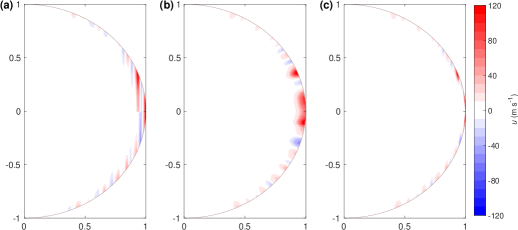
Figure 2: Options of cloud-level wind projection and decay profiles, shown for an example of a sharp decay at a 3000 km distance from the surface. (a) Projection in the direction parallel to the spin axis and decay in the radial direction. (b) Projection and decay in the radial direction. (c) Projection and decay in the direction parallel to the spin axis.

Given a zonal flow structure, thermal wind balance is used to calculate an anomalous density structure associated with large-scale flow in fast rotating gas giants. The density field is then integrated to give the 1-bar gravity field in terms of the zonal gravity harmonics (Kaspi et al., 2010). Using an adjoint based optimization, a solution for the flow structure is searched for, such that the model solution for the gravity field is best fitted to the part of the measured gravity field that can be attributed to the wind (Galanti and Kaspi, 2016). The odd gravity harmonics are attributed solely to the wind, therefore we use the Juno measured values $J_{3}=(-4.24\pm 0.91)\times 10^{-8}$, $J_{5}=(-6.89\pm 0.81)\times 10^{-8}$, $J_{7}=(12.39\pm 1.68)\times 10^{-8}$, and $J_{9}=(-10.58\pm 4.35)\times 10^{-8}$ (Iess et al., 2018). The lowest even harmonics $J_{2}$ and $J_{4}$ are dominated by the planet’s density structure and shape and cannot be used in our analysis, but interior models can give a reasonable estimate for the expected wind contribution for the higher even harmonics $J_{6}$, $J_{8}$, and $J_{10}$ (Guillot et al., 2018). Based on the Juno measurements and the range of interior model solutions, the expected wind-induced even harmonics are estimated as $\Delta J_{6}=1\times 10^{-8}\pm(0.9+2)\times 10^{-8}$, $\Delta J_{8}=3.5\times 10^{-8}\pm(2.46+0.5)\times 10^{-8}$, and $\Delta J_{10}=-3\times 10^{-8}\pm(6.94+0.25)\times 10^{-8}$. Note that the uncertainty associated with each even harmonic has contributions from both the measurement and the range of interior model solutions (first and second uncertainties, respectively). The large uncertainties in the estimated wind-induced even harmonics suggest that our analysis is limited to their order of magnitude and sign.

Finally, in order to isolate the latitudinal dependence from the general ability to fit the gravity harmonics, we first optimize the cloud-level wind so that the odd gravity harmonics are fitted perfectly (Galanti and Kaspi, 2021). The modified wind is very similar to the observed (Fig. S1), well within the uncertainty of the cloud-level wind observation (Tollefson et al., 2017), therefore retaining all the observed latitudinal structure responsible for the wind-induced gravity harmonics.

3 The latitudinal sensitivity of the wind-induced gravity field

We begin by analyzing the effect of the cloud-level wind latitudinal truncation on the ability to explain the gravity harmonics. For each wind setup, the internal flow structure is modified until the best fit to the 4 odd harmonics and the 3 even harmonics is reached (Fig. 3). The cost-function (Fig. 3a), a measure for the overall difference between the measurements and the model solution (see SI), reveals the contribution of each latitudinal region to the solution. First, as expected, when the cloud-level wind is retained at all latitudes, the solution for the odd harmonics is very close to the measurements (Fig. 3b-d, red dots). Importantly, the same optimal flow structure explains very well the even harmonics (Fig. 3e-f, red dots). This is additional evidence that the observed cloud-level wind is dynamically related to the gravity field.

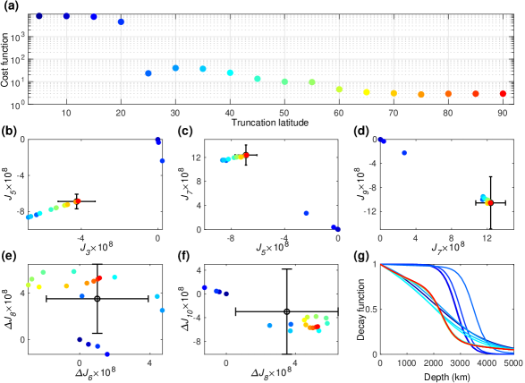
Figure 3: Latitude-dependent solutions as function of the truncation latitude. (a) The overall fit of the model solution to the measurements (cost function). Each case is assigned with a different color that is used in the following panels, ranging from latitude 5^∘ (blue) to 90^∘ (no truncation, red). (b-f) the solutions for the different gravity harmonics (colors), and the measurement (black). (g) the decay function associated with each solution.

Examining the latitudinal dependence of the truncation, it is evident that truncating the observed cloud-level wind closer to the equator than $25^{\circ}{\rm S}-25^{\circ}{\rm N}$ prevents any flow structure that could explain the gravity harmonics. It is most apparent in the odd harmonics (Fig. 3b-d) where the optimal solutions (dark blue circles) are close to zero and far from the measured values. It is also the case for $\Delta J_{8}$ , but for $\Delta J_{6}$ and $\Delta J_{10}$ the solutions are always inside the uncertainty: in $\Delta J_{6}$ because the measured value is very small, and in $\Delta J_{10}$ because the uncertainty is very large. Considering the cloud-level wind profile (Fig. 1a, black), it is not surprising that truncating the winds poleward of $25^{\circ}{\rm S}-25^{\circ}{\rm N}$ makes the difference in the solution, as this is where the positive (negative) jet in the northern (southern) hemisphere are found, and project strongly on the low order odd harmonics. Note that even a 5^∘ difference (Fig. 1a, red, truncation at $20^{\circ}{\rm S}-20^{\circ}{\rm N}$) prevents a physical solution from being reached. Once these opposing jets are included, the flow structure contains enough asymmetry to explain very well $J_{7}$ and $J_{9}$ which have the largest values of the odd harmonics.

However, with the $25^{\circ}{\rm S}-25^{\circ}{\rm N}$ truncation, the model solutions for $J_{3}$ and $J_{5}$ are still outside the measured uncertainty. Only when the influence of the zonal winds throughout the $50^{\circ}{\rm S}-50^{\circ}{\rm N}$ range (Fig. 1a, cyan) is included, then the lower odd harmonics can be explained with the cloud-level wind profile. The optimal decay function for each case (Fig. 3g), emphasize the robustness of the solutions. When only the equatorial region is retained, the optimization is trying (with no success) to include as much mass in the region where the cloud-level wind is projected inward. But once the winds at $25^{\circ}{\rm S}-25^{\circ}{\rm N}$ are included, then the decay function of the wind settles on a similar profile, with some small variations between the cases. Note that repeating these experiments with the exact Tollefson et al. (2017) cloud-level wind profile, does not change substantially the main results (Fig. S2), thus ensuring the robustness of the results.

The same methodology can be applied to a cloud-level wind that is truncated equatorward of a latitudinal region (Fig. S3). The analysis shows that a wind truncated equatorward of a latitude larger than $25^{\circ}{\rm S}-25^{\circ}{\rm N}$ does not allow a plausible solution to be reached. Consistently with the above experiment, the deep jets at $25^{\circ}{\rm S}-25^{\circ}{\rm N}$ are necessary to fit gravity harmonics. Specifically, there is a gradual deterioration of the solution in the truncation region of 0^∘ to 20^∘, which is related solely to the even harmonics $\Delta J_{6}$ , $\Delta J_{8}$, and $\Delta J_{10}$. Once the wind is truncated inside 10^∘S-10^∘N the solution for $\Delta J_{6}$ and $\Delta J_{8}$ is outside the uncertainty range, and $\Delta J_{10}$ moves further away from the measurement. This is due to the strong eastward jets at 6^∘S and 6^∘N.

4 Variants of the flow structure

Next, we examine several variants to the wind setups. In section 3 we showed that the jets between 25^∘S and 25^∘N are crucial for explaining the gravity harmonics, and therefore should not differ much below the cloud level. However, in the regions where the wind is truncated it should be examined whether a flow below the cloud level that is completely different might still allow matching the gravity harmonics. We therefore examine a case where the cloud-level wind is truncated poleward of $25^{\circ}{\rm S}-25^{\circ}{\rm N}$, and in the truncated regions random jets are added to simulate different possible scenarios (Fig. 1b, see SI for definition). The gravity harmonic solutions for 1000 different cases is shown in Fig. 4 (a-c). The largest effect the random jets have is on $J_{3}$ and $J_{5}$, with considerable effect also on the other odds and even harmonics. About 4% of the cases provide a good match to all the measurements (green), therefore it is statistically possible that some combination of jets unseen at the cloud level at the mid-latitudes, with amplitude of up to $\pm 40$ m s^-1, are responsible for part of the gravity signal. Doubling (halving) the random jets strength results in only 1.1% (1.2%) of the solutions to fit the gravity measurement (SI, Fig. S7), suggesting that if alternative jets exists in the mid-latitudes, their amplitude should be around $\pm 40$ m s^-1. These results are consistent with Duer et al. (2020) who did a similar analysis, but taking the full cloud level winds and showed that solutions differing from the cloud level are possible but statistically unlikely ($\sim 1\%$).

Figure 4: (a-c) Solutions with the cloud-level wind truncated poleward of $25^{\circ}{\rm S}-25^{\circ}{\rm N}$ and replaced with random jets there (Fig. 1b). Shown are the solutions for 1000 random cases (gray), and within those the solution which matches all the gravity harmonics (green). Also shown are the solution with no random winds (blue, corresponding to the 25^∘ case in Fig. 3), the solution with no truncation of the winds (red, corresponding to the 90^∘ case in Fig. 3) and the Juno measurements (black). (d) Solutions for cases with cloud-level wind projected in the radial direction (blue; Fig. 2b) and wind decayed in the direction parallel to the spin axis (magenta; Fig. 2c), and a doubled cloud-level wind (green). Also shown are the measurements (black), and the solution with the unaltered cloud-level wind (red; Kaspi et al., 2018).

Aside from modifications to the cloud-level wind, we also examine cases in which the projection of the flow beneath the cloud level is modified. For simplicity, we examine these cases with the observed cloud-level wind spanning the full latitudinal range. Projecting the wind radially and keeping the decay radial (Fig. 2b), we find that there is no plausible solution for flow structure under these assumptions that would give a good fit to the gravity measurements (Fig. 4d, blue). The best-fit model solution for all $J_{n}$ is far from the measurements, well outside their uncertainty range, and does not even match $J_{3}$ in sign. Next, we consider a case in which the decay of the winds is in the direction parallel to the spin axis (Fig. 2c). Here the optimal solution for the odd harmonics is far from the measured values (Fig. 4d, magenta), while for the even harmonics the solution is within the uncertainty range. However, in this case the winds needs to be very deep, extending to $\sim 5000$ km, where the interaction with the magnetic field is extremely strong (Cao and Stevenson, 2017; Galanti et al., 2017; Galanti and Kaspi, 2021). Finally, following the suggestion that the cloud-level wind might get stronger with depth before they decay (e.g., Fletcher et al., 2021), we conduct an experiment in which we double the cloud-level wind. Interestingly, a plausible solution can be achieved (Fig. 4d, green crosses), with a decay profile similar to the Kaspi et al. (2018) solution, but with the winds decaying more baroclinicaly in the upper 2000 km, and then decaying slower (Fig. S6).

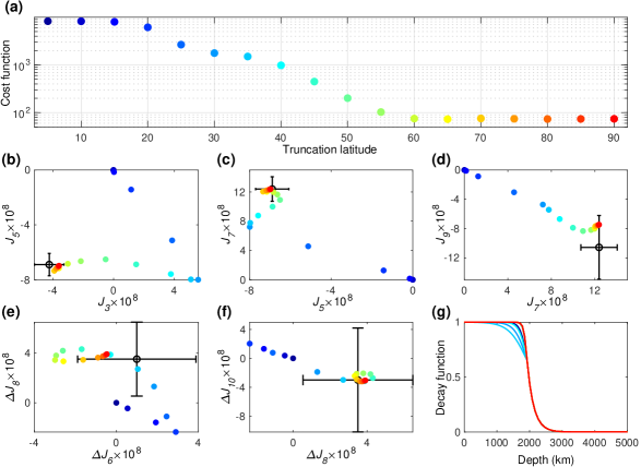
Figure 5: Same as Fig. 3, but for a case where the flow profile in the semiconducting region is restricted to comply with secular variations consideration.

5 Adding magnetohydrodynamic constraints

In Jupiter, the increased conductivity with depth (e.g., French et al., 2012; Wicht et al., 2019) suggests that the flow might be reduced to very small values in the semiconducting region (deeper than 2000 km, Cao and Stevenson, 2017). Using flow estimates in the semiconducting region based on past magnetic secular variations (Moore et al., 2019), Galanti and Kaspi (2021) gave a revised wind decay profile that can explain both the gravity harmonics and the constraints posed by the secular variations. We follow this approach, setting the flow strength in the semiconducting region (deeper than 2000 km, see Galanti and Kaspi, 2021) to be a sharp exponential function (Fig. 5g, right part). Given this inner profile of the decay function, the outer part of the decay function can be searched for, together with the optimal cloud-level wind, that will result in the best fit to the odd measured gravity harmonics. The optimal cloud-level wind (Fig. S1b) is very similar to the observed wind, with deviations that are within the uncertainties.

Using the modified cloud-level wind, the shape of the decay function in the outer neutral region is optimized to allow the best-fit to the odd and even gravity harmonics (Fig. 5b-g). In addition to the odd harmonics, which are expected to fit the measurements, the model also fits very well the even harmonics, despite the limited range of possible decay profiles in the outer region (Fig. 5g). The latitudinal dependence reveals that the range of $50^{\circ}{\rm S}-50^{\circ}{\rm N}$ is needed in order to allow a good fit, especially for $J_{3}$ and $J_{7}$. Similar to the case with gravity-only constraints, fitting the even harmonics, as well as $J_{5}$ and $J_{9}$., requires mostly the cloud-level wind inside the $25^{\circ}{\rm S}-25^{\circ}{\rm N}$ region. Thus, even when including the strong magnetic constraint, the dominance of the $25^{\circ}{\rm S}-25^{\circ}{\rm N}$ region remains robust.

References

- Atkinson et al. (1998) Atkinson, D. H., J. B. Pollack, and A. Seiff, The Galileo probe doppler wind experiment: Measurement of the deep zonal winds on Jupiter, J. Geophys. Res., 103, 22,911–22,928, doi:10.1029/98JE00060, 1998.
- Bolton et al. (2017) Bolton, S. J., et al., Jupiter’s interior and deep atmosphere: The initial pole-to-pole passes with the Juno spacecraft, Science, 356, 821–825, doi:10.1126/science.aal2108, 2017.
- Busse (1970) Busse, F. H., Thermal instabilities in rapidly rotating systems, J. Fluid Mech., 44, 441–460, doi:10.1017/S0022112070001921, 1970.
- Busse (1976) Busse, F. H., A simple model of convection in the Jovian atmosphere, Icarus, 29, 255–260, doi:10.1016/0019-1035(76)90053-1, 1976.
- Busse (1994) Busse, F. H., Convection driven zonal flows and vortices in the major planets, Chaos, 4(2), 123–134, doi:10.1063/1.165999, 1994.
- Cao and Stevenson (2017) Cao, H., and D. J. Stevenson, Zonal flow magnetic field interaction in the semi-conducting region of giant planets, Icarus, 296, 59–72, doi:10.1016/j.icarus.2017.05.015, 2017.
- Choi et al. (2013) Choi, D. S., A. P. Showman, A. R. Vasavada, and A. A. Simon-Miller, Meteorology of Jupiter’s equatorial hot spots and plumes from Cassini, Icarus, 223(2), 832–843, doi:10.1016/j.icarus.2013.02.001, 2013.
- Christensen (2001) Christensen, U. R., Zonal flow driven by deep convection in the major planets, Geophys. Res. Lett., 28, 2553–2556, doi:10.1029/2000GL012643, 2001.
- Christensen et al. (2020) Christensen, U. R., J. Wicht, and W. Dietrich, Mechanisms for Limiting the Depth of Zonal Winds in the Gas Giant Planets, Astrophys. J., 890(1), 61, doi:10.3847/1538-4357/ab698c, 2020.
- Debras and Chabrier (2019) Debras, F., and G. Chabrier, New models of Jupiter in the context of Juno and Galileo, Astrophys. J., 872, 100–, doi:10.3847/1538-4357/aaff65, 2019.
- Dowling (1995) Dowling, T. E., Estimate of Jupiter’s deep zonal-wind profile from Shoemaker-Levy 9 data and Arnold’s second stability criterion, Icarus, 117, 439–442, doi:10.1006/icar.1995.1169, 1995.
- Dowling (2020) Dowling, T. E., Jupiter-style Jet Stability, The Planatary Science Journal, 1, 6, doi:10.3847/PSJ/ab789d, 2020.
- Duer et al. (2019) Duer, K., E. Galanti, and Y. Kaspi, Analysis of Jupiter’s deep jets combining Juno gravity and time-varying magnetic field measurements, Astrophys. J. Let., 879(2), L22, doi:10.3847/2041-8213/ab288e, 2019.
- Duer et al. (2020) Duer, K., E. Galanti, and Y. Kaspi, The Range of Jupiter’s Flow Structures that Fit the Juno Asymmetric Gravity Measurements, J. Geophys. Res. (Planets), 125(8), e06292, doi:10.1029/2019JE006292, 2020.
- Fletcher et al. (2020) Fletcher, L. N., Y. Kaspi, T. Guillot, and A. P. Showman, How Well Do We Understand the Belt/Zone Circulation of Giant Planet Atmospheres?, Space Sci. Rev., 216(2), 30, doi:10.1007/s11214-019-0631-9, 2020.
- Fletcher et al. (2021) Fletcher, L. N., et al., Jupiter’s temperate belt/zone contrasts revealed at depth by Juno microwave observations, submitted, 2021.
- French et al. (2012) French, M., A. Becker, W. Lorenzen, N. Nettelmann, M. Bethkenhagen, J. Wicht, and R. Redmer, Ab initio simulations for material properties along the Jupiter adiabat, Astrophys. J. Sup., 202(1), 5, doi:10.1088/0067-0049/202/1/5, 2012.
- Galanti and Kaspi (2016) Galanti, E., and Y. Kaspi, An Adjoint-based Method for the Inversion of the Juno and Cassini Gravity Measurements into Wind Fields, Astrophys. J., 820(2), 91, doi:10.3847/0004-637X/820/2/91, 2016.
- Galanti and Kaspi (2021) Galanti, E., and Y. Kaspi, Combined magnetic and gravity measurements probe the deep zonal flows of the gas giants, MNRAS, 501(2), 2352–2362, doi:10.1093/mnras/staa3722, 2021.
- Galanti et al. (2017) Galanti, E., H. Cao, and Y. Kaspi, Constraining Jupiter’s internal flows using Juno magnetic and gravity measurements, Geophys. Res. Lett., 44(16), 8173–8181, doi:10.1002/2017GL074903, 2017.
- Guillot et al. (2018) Guillot, T., et al., A suppression of differential rotation in Jupiter’s deep interior, Nature, 555, 227–230, doi:10.1038/nature25775, 2018.
- Heimpel et al. (2016) Heimpel, M., T. Gastine, and J. Wicht, Simulation of deep-seated zonal jets and shallow vortices in gas giant atmospheres, Nature Geoscience, 9, 19–23, doi:10.1038/ngeo2601, 2016.
- Iess et al. (2018) Iess, L., et al., Measurement of Jupiter’s asymmetric gravity field, Nature, 555, 220–222, doi:10.1038/nature25776, 2018.
- Ingersoll et al. (2017) Ingersoll, A. P., et al., Implications of the ammonia distribution on Jupiter from 1 to 100 bars as measured by the Juno microwave radiometer, Geophys. Res. Lett., 44(15), 7676–7685, doi:10.1002/2017GL074277, 2017.
- Janssen et al. (2017) Janssen, M. A., et al., MWR: Microwave Radiometer for the Juno Mission to Jupiter, Space Sci. Rev., 213(1-4), 139–185, doi:10.1007/s11214-017-0349-5, 2017.
- Kaspi (2013) Kaspi, Y., Inferring the depth of the zonal jets on Jupiter and Saturn from odd gravity harmonics, Geophys. Res. Lett., 40, 676–680, doi:10.1029/2009GL041385, 2013.
- Kaspi et al. (2009) Kaspi, Y., G. R. Flierl, and A. P. Showman, The deep wind structure of the giant planets: Results from an anelastic general circulation model, Icarus, 202(2), 525–542, doi:10.1016/j.icarus.2009.03.026, 2009.
- Kaspi et al. (2010) Kaspi, Y., W. B. Hubbard, A. P. Showman, and G. R. Flierl, Gravitational signature of Jupiter’s internal dynamics, Geophys. Res. Lett., 37, L01,204, doi:10.1029/2009GL041385, 2010.
- Kaspi et al. (2020) Kaspi, Y., E. Galanti, A. P. Showman, D. J. Stevenson, T. Guillot, L. Iess, and S. J. Bolton, Comparison of the Deep Atmospheric Dynamics of Jupiter and Saturn in Light of the Juno and Cassini Gravity Measurements, Space Sci. Rev., 216(5), 84, doi:10.1007/s11214-020-00705-7, 2020.
- Kaspi et al. (2018) Kaspi, Y., et al., Jupiter’s atmospheric jet streams extend thousands of kilometres deep, Nature, 555, 223–226, doi:10.1038/nature25793, 2018.
- Kong et al. (2018) Kong, D., K. Zhang, G. Schubert, and J. D. Anderson, Origin of Jupiter’s cloud-level zonal winds remains a puzzle even after Juno, Proc. Natl. Acad. Sci. U.S.A., 115(34), 8499–8504, doi:10.1073/pnas.1805927115, 2018.
- Li et al. (2017) Li, C., et al., The distribution of ammonia on Jupiter from a preliminary inversion of Juno microwave radiometer data, Geophys. Res. Lett., 44(11), 5317–5325, doi:10.1002/2017GL073159, 2017.
- Li et al. (2020) Li, C., et al., The water abundance in Jupiter’s equatorial zone, Nature Astronomy, 4, 609–616, doi:10.1038/s41550-020-1009-3, 2020.
- Li et al. (2006) Li, L., A. P. Ingersoll, A. R. Vasavada, A. A. Simon-Miller, A. D. Del Genio, S. P. Ewald, C. C. Porco, and R. A. West, Vertical wind shear on Jupiter from Cassini images, J. Geophys. Res. (Planets), 111(E4), E04004, doi:10.1029/2005JE002556, 2006.
- Liu et al. (2008) Liu, J., P. M. Goldreich, and D. J. Stevenson, Constraints on deep-seated zonal winds inside Jupiter and Saturn, Icarus, 196, 653–664, doi:10.1016/j.icarus.2007.11.036, 2008.
- Moore et al. (2019) Moore, K. M., H. Cao, J. Bloxham, D. J. Stevenson, J. E. P. Connerney, and S. J. Bolton, Time variation of Jupiter’s internal magnetic field consistent with zonal wind advection, Nature Astronomy, 3, 730–735, doi:10.1038/s41550-019-0772-5, 2019.
- Orton et al. (1998) Orton, G. S., et al., Characteristics of the Galileo probe entry site from earth-based remote sensing observations, J. Geophys. Res., 103, 22,791–22,814, doi:10.1029/98JE02380, 1998.
- Tollefson et al. (2017) Tollefson, J., et al., Changes in Jupiter’s zonal wind profile preceding and during the Juno mission, Icarus, 296, 163–178, doi:10.1016/j.icarus.2017.06.007, 2017.
- Wicht et al. (2019) Wicht, J., T. Gastine, L. D. V. Duarte, and W. Dietrich, Dynamo action of the zonal winds in Jupiter, Astron. and Astrophys., 629, A125, doi:10.1051/0004-6361/201935682, 2019.