February 21, 2021

Solution of the Basel problem
in the framework of distribution theory Andreas Aste
Department of Physics, University of Basel,
Klingelbergstrasse 82, CH-4056 Basel, Switzerland
E-Mail: andreas.aste@unibas.ch

A simple proof of Euler’s formula which states that the sum of the reciprocals of all natural numbers squared equals $\pi^{2}/6$ is presented based on the distribution theory introduced by Laurent Schwartz. Additional identities are obtained as a byproduct of the derivation.

Mathematics Subject Classification MSC 2010: 40A25, 46F05
Keywords: Basel problem; Zeta function; distribution theory; generalized functions; test functions; summation of series

1 Introduction

The so-called Basel problem to determine the sum $\zeta(2)=\sum_{n=1}^{\infty}\frac{1}{n^{2}}=\pi^{2}/6$ was first posed in 1644 by Pietro Mengoli, an Italian mathematician and clergyman from Bologna, and solved by the Swiss mathematician Leonhard Euler (*1707 in Basel, ^†1783 in Saint Petersburg) in 1735. Several ways have been found in the meantime to calculate $\zeta(2)$ (see [2] and references therein). A further simple method to derive Euler’s result using the the theory of distributions and test functions which is based on elementary arguments like translational invariance is presented in this letter.

Distribution theory [1], which represents a mathematical discipline in its own right, is of fundamental significance for a rigourous treatment of quantum field theories in classical spacetime [3, 4]. It is also hoped that the stunning exercise presented in this letter serves as an incentive for graduate students with some basic knowledge of distribution theory to study the subject of generalized functions and their applications in theoretical physics in greater detail.

2 Calculating $\zeta(2)$

We consider the distribution $\Delta_{0}\in\mathcal{D}^{\prime}(\mathds{R})$ defined by the formal expression

$$\Delta_{0}(x)=\sum\limits_{n=-\infty}^{\infty}e^{inx}=\ldots+e^{-3ix}+e^{-2ix}+e^{-x}+1+e^{ix}+e^{2ix}+e^{3ix}+\ldots\,,$$ (1)

which acts on (smooth) test functions (with compact support) $\varphi\in\mathcal{D}(\mathds{R})$ as a linear and, in the sense of distributions, continuous functional according to

$$\Delta_{0}[\varphi]:=\sum\limits_{n=-\infty}^{\infty}\int\limits_{-\infty}^{\infty}e^{inx}\varphi(x)dx=\lim_{N\rightarrow\infty}\sum\limits_{n=-N}^{N}\int\limits_{-\infty}^{\infty}e^{inx}\varphi(x)dx\,.$$ (2)

In fact, $\Delta_{0}$ is well-defined by equation (2) as a distribution in $\mathcal{D}^{\prime}(\mathds{R})$, the dual space of $\mathcal{D}(\mathds{R})$, and equation (2) highlights the meaning of the formal definition (1) of $\Delta_{0}$ as a generalized function [6]. Note that a more intuitive representation of $\Delta_{0}$ as an alternative infinite sum of Dirac delta distributions is motivated in the appendix.

By definition, $\Delta_{0}$ is a periodic distribution invariant under a translation $T_{2\pi}$, i.e. formally

$$(T_{2\pi}\Delta_{0})(x)=\Delta_{0}(x+2\pi)=\sum\limits_{n=-\infty}^{\infty}e^{in(x+2\pi)}=\sum\limits_{n=-\infty}^{\infty}e^{inx}=\Delta_{0}(x)\,,$$ (3)

or in distributional notation

$$(T_{2\pi}\Delta_{0})[\varphi]=\Delta_{0}[T_{2\pi}\varphi]\quad\forall\varphi\in\mathcal{D}(\mathds{R})\,,\quad\mbox{where}\,\,\,(T_{2\pi}\varphi)(x)=\varphi(x-2\pi)\,,$$ (4)

and $\Delta_{0}$ is symmetric

$$\Delta_{0}(x)=\Delta_{0}(-x)\,.$$ (5)

Now since $\Delta_{0}(x)$ is invariant with respect to a multiplication with $e^{ix}$, i.e.

$$e^{ix}\Delta_{0}(x)=e^{ix}\sum\limits_{n=-\infty}^{\infty}e^{inx}=\sum\limits_{n=-\infty}^{\infty}e^{inx}\,,$$ (6)

$\Delta_{0}$ must vanish as a distribution on $\mathds{R}\backslash\{2\pi n\,|\,n\in\mathds{Z}\}$, since only for $x=2\pi n$ with $n\in\mathds{Z}$ one has a trivial factor $e^{ix}=1$; therefore the distributional support of $\Delta_{0}$ must be contained in a corresponding discrete set

$$supp\,\Delta_{0}\subseteq\{2\pi n\,|\,n\in\mathds{Z}\}\,.$$ (7)

For a moment, the following considerations are restricted to the open interval $I=(0,2\pi)$. Calculating the first antisymmetric antiderivative $\Delta_{1}$ of $\Delta_{0}$ with $x\in I$

$$\Delta_{1}(x)=\lim_{\epsilon\searrow 0}\int\limits_{\epsilon}^{x}\Delta_{0}(x^{\prime})dx^{\prime}=-i\sum\limits_{\begin{subarray}{c}n=-\infty\\ n\neq 0\end{subarray}}^{\infty}\frac{e^{inx}}{n}+x=2\sum\limits_{n=1}^{\infty}\frac{\sin(nx)}{n}+x$$ (8)

with

$$\Delta_{1}(x)=-\Delta_{1}(-x)\,,$$ (9)

$\Delta_{1}$ must be constant on $I$, since its derivative $\Delta_{0}$ vanishes there. This also implies that the Fourier sum in equation (8) represents a linear function on $I$. Calculating the mean value $\mu_{I,1}$ of $\Delta_{1}$ on $I$ according to

$$\mu_{I,1}=\frac{1}{2\pi}\lim_{\epsilon\searrow 0}\int\limits_{\epsilon}^{2\pi-\epsilon}\Delta_{1}(x)dx\,,$$ (10)

the oscillatory terms $\sim e^{inx}$ in equation (8) do not contribute to $\mu_{I,1}$ and one is left with

$$\mu_{I,1}=\frac{1}{2\pi}\int\limits_{0}^{2\pi}xdx=\pi\,.$$ (11)

Finally turning to the antiderivative of $\Delta_{1}$ on $I$

$$\Delta_{2}(x)=\int\limits_{0}^{x}\Delta_{1}(x^{\prime})dx^{\prime}=-\sum\limits_{n\in\mathds{Z}\backslash 0}\frac{e^{inx}}{n^{2}}+\frac{1}{2}x^{2}=-2\sum\limits_{n=1}^{\infty}\frac{\cos(nx)}{n^{2}}+\frac{1}{2}x^{2}\,,$$ (12)

one arrives at an expression containing a series that converges absolutely to a continuous function on $I$. However, since the distributional derivative of $\Delta_{2}$ is $\Delta_{1}$ which is constant, i.e., $\pi$ on $I$, $\Delta_{2}$ must be of the form

$$\Delta_{2}(x)=\pi x+\gamma\,,\quad x\in I$$ (13)

with an integration constant $\gamma$. This constant can be calculated by considering the average value of $\Delta_{2}$ on $I$

$$\mu_{I,2}=\frac{1}{2\pi}\int\limits_{0}^{2\pi}x^{2}\frac{dx}{2}=\frac{2\pi^{2}}{3}=\frac{1}{2\pi}\int\limits_{0}^{2\pi}(\pi x+\gamma)dx=\pi^{2}+\gamma\,,$$ (14)

hence $\gamma=-\pi^{2}/3$, an finally Euler’s famous result

$$\Delta_{2}(0)=-2\sum\limits_{n=1}^{\infty}\frac{1}{n^{2}}=\gamma=-\frac{\pi^{2}}{3}\,\,\rightarrow\,\,\sum\limits_{n=1}^{\infty}\frac{1}{n^{2}}=\frac{\pi^{2}}{6}$$ (15)

follows.

As an exercise, the reader may verify that by considering additional antiderivatives of $\Delta_{2}$ like $\Delta_{4}$, $\Delta_{6}$ et cetera, further values of the Euler-Riemann zeta function like

$$\zeta(4)=\sum\limits_{n=1}^{\infty}\frac{1}{n^{4}}=\frac{\pi^{4}}{90}\,,\quad\zeta(6)=\sum\limits_{n=1}^{\infty}\frac{1}{n^{6}}=\frac{\pi^{6}}{945}\,,\quad\ldots$$ (16)

follow directly from strategy outlined above.

Appendix A Explicit representation of $\Delta_{0}$ as an infinite sum of Dirac delta distributions

We consider the following sequence $\{\delta_{N}\}_{N\in\mathds{N}_{0}}\subset\mathcal{D}^{\prime}(\mathds{R})$ of distributions [6] represented by the functions

$$\delta_{N}(x)=\Theta(\pi^{2}-x^{2})\sum\limits_{n=-N}^{N}e^{inx}=\begin{cases}\sum\limits_{n=-N}^{N}e^{inx}&|x|<\pi\\ 0&|x|\geq\pi\end{cases}$$ (17)

with $supp\,\delta_{N}=[-\pi,\pi]$, where

$$\Theta(x)=\begin{cases}1&x>0\\ 0&x\leq 1\end{cases}$$ (18)

is the Heaviside function. With $\delta_{N}(x)=e^{-iNx}+e^{-i(N-1)x}+\ldots+e^{-ix}+1+e^{ix}+\ldots+e^{iNx}$ and

$$e^{ix}\delta_{N}(x)=\delta_{N}(x)+e^{i(N+1)x}-e^{-iNx}$$ (19)

for $x\in(-\pi,\pi)$ one immediately obtains the compact representation

$$\delta_{N}(x)=\frac{e^{i(N+1)x}-e^{-iNx}}{e^{ix}-1}=\frac{e^{i(N+1/2)x}-e^{-i(N+1/2)x}}{e^{ix/2}-e^{-ix/2}}=\frac{\sin((N+1/2)x)}{\sin(x/2)}\,,\quad x\in(-\pi,\pi)\backslash\{0\}$$ (20)

and from the definition (17) one has $\delta_{N}(0)=2N+1$ which removes the singularity appearing at $x=0$ in the representation (20). Only the term $e^{i0x}=1$ in definition (17) contributes to the integral

$$\int\limits_{-\infty}^{\infty}\delta_{N}(x)dx=\int\limits_{-\pi}^{\pi}\delta_{N}(x)dx=2\pi\,.$$ (21)

For illustrative purposes, the graph of $\delta_{50}$ is depicted in Fig. 1.

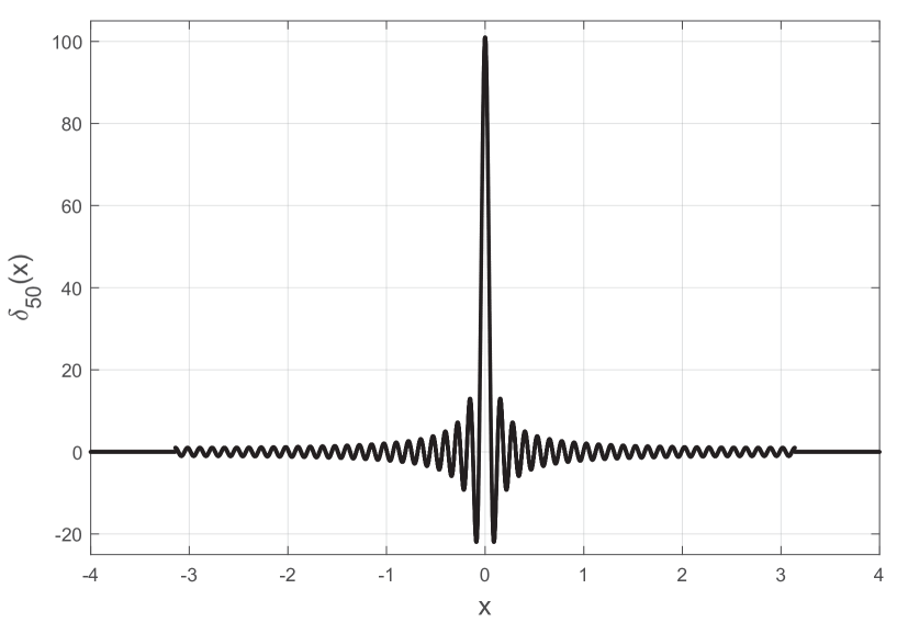
Figure 1: The graph of $\delta_{50}$ defined by equation (17).

In fact, $\{\delta_{N}\}_{N\in\mathds{N}_{0}}\subset\mathcal{D}^{\prime}(\mathds{R})$ is a $\delta$-sequence converging to $2\pi$ times the Dirac delta distribution $\delta$ for $N\rightarrow\infty$. Applying $\delta_{N}$ on a (smooth) test function $\varphi\in\mathcal{D}(\mathds{R})$ (with compact support) leads to

$$\delta_{N}[\varphi]=\int\limits_{-\infty}^{\infty}\delta_{N}(x)\varphi(x)dx=\int\limits_{-\pi}^{\pi}\frac{\sin((N+1/2)x)}{\sin(x/2)}\varphi(x)dx$$

$$=2\int\limits_{-\pi}^{\pi}\frac{\sin((N+1/2)x)}{x}\frac{x/2}{\sin(x/2)}\varphi(x)dx=2\int\limits_{-\pi}^{\pi}\frac{\sin((N+1/2)x)}{x}\beta(x)\frac{x/2}{\sin(x/2)}\varphi(x)dx$$ (22)

where a smooth bump function $\beta\in\mathcal{D}(\mathds{R})$ with the properties $\beta(x)=1$ for $|x|\leq\pi$ and $\beta(x)=0$ for $|x|\geq 3\pi/2$ was introduced which does not change the integral above. Since one has

$$\sigma(x)=\begin{cases}\frac{1}{{\rm{si}}(x/2)}=\frac{x/2}{\sin(x/2)}&|x|\in(0,3\pi/2]\\ 1&x=0\end{cases}\,,\quad\sigma\in C^{\infty}([-3\pi/2,3\pi/2])\,,$$ (23)

i.e. since $\sigma$ is a smooth function on the interval $[-3\pi/2,3\pi/2]$, also $\tilde{\varphi}(x)=\beta(x)\sigma(x)\varphi(x)$ is smooth and has compact support: $\tilde{\varphi}\in\mathcal{D}(\mathds{R})$. Furthermore, $\tilde{\varphi}(0)=\varphi(0)$ holds.

Now, equation (22) becomes, with $x^{\prime}=(N+1/2)x$ in the limit $N\rightarrow\infty$ in the sense of distributions

$$\delta_{N}[\varphi]=\int\limits_{-\infty}^{\infty}\delta_{N}(x)\varphi(x)dx=2\int\limits_{-\pi}^{\pi}\frac{\sin((N+1/2)x)}{x}\tilde{\varphi}(x)dx=2\int\limits_{-(N+1/2)\pi}^{(N+1/2)\pi}\frac{\sin(x^{\prime})}{x^{\prime}}\tilde{\varphi}(x^{\prime}/(N+1/2))dx^{\prime}$$

$$\,\xrightarrow{N\rightarrow\infty}\,2\int\limits_{-\infty}^{\infty}\frac{\sin(x^{\prime})}{x^{\prime}}\tilde{\varphi}(0)dx^{\prime}=2\pi\tilde{\varphi}(0)=2\pi\varphi(0)=2\pi\delta[\varphi]\,.$$ (24)

The normalization of the $\delta$-distribution follows from equation (21), i.e., as a byproduct of the derivation presented above the integral

$$\lim_{N\rightarrow\infty}\int\limits_{-(N+1/2)\pi}^{(N+1/2)\pi}\frac{\sin(x)}{x}dx=\int\limits_{-\infty}^{\infty}\frac{\sin(x)}{x}dx=\pi$$ (25)

is obtained. Neglecting the cutoff in definition (17) leads to the periodic distributional identity

$$\Delta_{0}(x)=\sum\limits_{n=-\infty}^{\infty}e^{inx}=2\pi\sum\limits_{n=-\infty}^{\infty}\delta(x-2\pi n)\quad\mbox{or}\quad\Delta_{0}[\varphi]=2\pi\sum\limits_{n=-\infty}^{\infty}\varphi(2\pi n)\,.$$ (26)

One readily expresses the antisymmetric antiderivative of $\Delta_{0}$ by the help of the floor function $\lfloor\cdot\rfloor$ and the ceiling function $\lceil\cdot\rceil$

$$\Delta_{1}(x)=\pi\biggl{(}\biggl{\lfloor}\frac{x}{2\pi}\biggr{\rfloor}+\biggl{\lceil}\frac{x}{2\pi}\biggr{\rceil}\biggl{)}\,,$$ (27)

which simplifies to

$$\Delta_{1}(x)=\pi\,\text{sign}(x)$$ (28)

on the open interval $(-2\pi,2\pi)$, and the symmetric antiderivative of $\Delta_{1}$ is represented by the continuous function

$$\Delta_{2}(x)=\pi x\biggl{(}\biggl{\lfloor}\frac{x}{2\pi}\biggr{\rfloor}+\biggl{\lceil}\frac{x}{2\pi}\biggr{\rceil}\biggl{)}-2\pi^{2}\biggl{(}\biggl{\lceil}\frac{x}{2\pi}\biggr{\rceil}\biggl{\lfloor}\frac{x}{2\pi}\biggr{\rfloor}\biggl{)}-\frac{\pi^{2}}{3}=-\sum\limits_{n\in\mathds{Z}\backslash\{0\}}\frac{e^{inx}}{n^{2}}+\frac{x^{2}}{2}\,.$$ (29)

References

• [1] Schwartz, L.: GΓ©nΓ©ralisation de la notion de fonction, de dΓ©rivation, de transformation de Fourier et applications mathΓ©matiques et physiques. Ann. Univ. Grenoble. Sect. Sci. Math. Phys. (N.S.) 21 (1945), pp. 57–74 (1945).
• [2] Riemenschneider, O.: Über einige elementare analytische Berechnungen von $\zeta(2)$. Variationen ΓΌber ein Thema von Leonhard Euler. Mitt. Math. Ges. Hamburg XXXXVI, pp. 53-69 (2016).
• [3] Streater, R.F., Wightman, A.S.: PCT, Spin, Statistics and All That. Benjamin-Cummings Publishing Company, 1964.
• [4] Scharf, G.: Finite Quantum Electrodynamics: The Causal Approach. Dover Books on Physics, 2014.
• [5] Epstein H., Glaser V.: The role of locality in perturbation theory. Annales PoincarΓ© Phys. Theor. A19, pp. 211-295 (1973).
• [6] Constantinescu, F.: Distributions and Their Applications in Physics. Pergamon Press, 1980.