Divergent Predictive States:
The Statistical Complexity Dimension of
Stationary, Ergodic Hidden Markov Processes

Abstract

Even simply-defined, finite-state generators produce stochastic processes that require tracking an uncountable infinity of probabilistic features for optimal prediction. For processes generated by hidden Markov chains the consequences are dramatic. Their predictive models are generically infinite-state. And, until recently, one could determine neither their intrinsic randomness nor structural complexity. The prequel, though, introduced methods to accurately calculate the Shannon entropy rate (randomness) and to constructively determine their minimal (though, infinite) set of predictive features. Leveraging this, we address the complementary challenge of determining how structured hidden Markov processes are by calculating their statistical complexity dimension—the information dimension of the minimal set of predictive features. This tracks the divergence rate of the minimal memory resources required to optimally predict a broad class of truly complex processes.

I Introduction

A delicate symbiotic relationship lives at the heart of highly complex systems—the intricate patterns these systems generate arise through an interplay between determinism and stochasticity. Despite progress identifying and measuring degrees of randomness and unpredictability, basic questions about this state of affairs remain. Specifically, how do we quantify “structure”? Can we detect a system’s emergent patterns and quantify their organization?

Clearly posing these questions and developing the tools to answer them required, over the recent decades, integrating Turing’s computation theory [1, 2, 3], Shannon’s information theory [4], and Kolmogorov’s dynamical systems theory [5, 6, 7, 8, 9]. Together they highlighted the central role that information—its generation, transmission, and storage—plays in the organization and functioning of complex systems. Drawing from this convergence, computational mechanics [10] introduced a definition of the structural complexity of stochastic processes—the statistical complexity, which measures the number and distribution of optimally-predictive features.

Answers to the randomness-structure dichotomy have been carefully detailed and successfully implemented for stochastic processes that can be optimally predicted with countably-many predictive features [11, 12, 13]. However, there are complex systems arising in many engineering, physical, and biological systems [14, 15, 16, 17, 18] that require an infinite number of predictive features. Somewhat soberingly, these truly complex systems are implicated in many natural phenomena, from the geophysics of earthquakes [19] and physiological measurements of neural avalanches [20] to semantics in natural language [21] and cascading failures in power transmission grids [22].

As first established by Blackwell in the 1950s [14], calculating the Shannon entropy rate of even apparently simple processes—such as those generated by a discrete time, $N$-state hidden Markov chain (HMC)—requires tracking an uncountably-infinite set of belief distributions over the HMC’s states. The following establishes that optimally predicting this class of processes requires using these belief distributions as predictive features. These feature sets, living on the $(N-1)$-simplex, are complex: generically highly ramified and self-similar, they are the support of similarly-complicated measures [23]. This renders prediction of even simply-defined processes very challenging. Probing their structure is even more difficult. Nevertheless, the broad popularity and application of HMCs—not only in the study of complex systems [10], but also in coding theory [24], stochastic processes [25], stochastic thermodynamics [26], speech recognition [27], computational biology [28, 29], epidemiology [30], and finance [31]—gives testimony to the ubiquity of truly complex systems, in both theory and nature.

Our recent work [32] addressed this state of affairs, showing how to produce infinite sets of predictive features and accurately calculate the entropy rate for processes generated by HMCs. This gave a new and efficient tool for consistently describing the randomness of truly complex systems. However, those results did not address the complementary side of the complex-system paradox—the structural aspect of the interplay between structure and randomness. Troublingly, for processes with uncountably-infinite sets of predictive features, the statistical complexity diverges, substantially circumscribing its usefulness as a metric of system organization. As we will show, quantifying the structure of these truly complex systems requires a new approach and new tools and methods.

Historically, the need for such a measure of divergent information storage and Blackwell’s discovery were perhaps anticipated by Shannon’s definition in the 1940s of dimension rate [4]:

$$\lambda=\lim_{\delta\to 0}\lim_{\epsilon\to 0}\lim_{T\to\infty}\frac{N(\epsilon,\delta,T)}{T\log\epsilon}~{},$$

where $N(\epsilon,\delta,T)$ is the smallest number of elements that may be chosen such that all elements of a trajectory ensemble generated over time $T$, apart from a set of measure $\delta$, are within the distance $\epsilon$ of at least one chosen trajectory. This is the minimal “number of dimensions” required to specify a member of a trajectory (or message) ensemble. Unfortunately, Shannon devotes barely a paragraph to the concept, leaving it largely unmotivated and uninterpreted. Nonetheless, we take inspiration from this to develop the statistical complexity dimension, the asymptotic growth rate of the statistical complexity for an uncountably-infinite set of predictive features.

We conjecture that the statistical complexity dimension is the same dimension rate proposed by Shannon. However, the following goes beyond Shannon’s brief mention to provide constructive and accurate methods for determining this important system invariant. Technically, statistical complexity dimension is defined as the information dimension of the (self-similar set of) predictive states. Several distinct steps are involved. Determining this information dimension requires establishing ergodicity, calculating the Lyapunov spectrum of an HMC’s mixed-state presentation, and applying a suitably modified version of the Lyapunov-information dimension conjecture from dynamical systems that connects the spectrum to the dimension.

To highlight the usefulness of these informational quantities, that otherwise appear rather abstracted from natural systems, it should be noted that the following and its predecessor [32] were proceeded by two companion articles that applied the theoretical results here to two, rather different, physical domains. The first analyzed the origin of randomness and structural complexity engendered by quantum measurement [33]. The second solved a longstanding problem on exactly determining the thermodynamic functioning of Maxwellian demons, aka information engines [18]. That is, the predecessor and the present development (along with a sequel to be announced in the conclusion) lay out the mathematical and algorithmic tools required to successfully analyze structure and randomness in these applied problems. Taken together, we believe the new approach will find even wider use than in these application areas.

In the following, we introduce a practical and calculable measure of structural complexity analogous to Shannon’s dimension rate in the form of statistical complexity dimension $d_{\mu}$. Section II recalls the necessary background in stochastic processes, hidden Markov chains, and information theory. Section III recounts mixed states and their dynamic—the mixed-state presentation—as well as the connection to iterated function systems (IFSs) previously demonstrated. The main result follows in Sec. IV, where the Lyapunov-information dimension conjecture is reviewed and updated to our needs and the statistical complexity dimension $d_{\mu}$ is introduced. Finally, in Sec. VI $d_{\mu}$ of a three-state parametrized HMC is calculated across a wide region of parameter space, demonstrating the insights afforded by and computational efficiency of our methods.

II Hidden Markov Processes

Our main objects of study are stochastic processes and the mechanisms that generate them—hidden Markov chains, mixed states, and the $\epsilon$-machine. We touch on several of their important properties, including stationarity, ergodicity, randomness, and memory. The reader familiar with the previous work in this series [32] may skip to Section II.4.

II.1 Processes

A stochastic process $\mathcal{P}$ is a probability measure over a bi-infinite chain $\ldots\,{X}_{t-2}\,{X}_{t-1}\,{X}_{t}\,{X}_{t+1}\,{X}_{t+2}\ldots$ of random variables, each ${X}_{t}$ denoted by a capital letter. A particular realization $\ldots\,{x}_{t-2}\,{x}_{t-1}\,{x}_{t}\,{x}_{t+1}\,{x}_{t+2}\ldots$ is denoted via lowercase. We assume values ${x}_{t}$ belong to a discrete alphabet $\mathcal{A}$. We work with blocks ${X}_{t:t^{\prime}}$, where the first index is inclusive and the second exclusive: ${X}_{t:t^{\prime}}={X}_{t}\ldots{X}_{t^{\prime}-1}$. $\mathcal{P}$’s measure is defined via the collection of distributions over blocks: $\{\Pr({X}_{t:t^{\prime}}):t<t^{\prime},t,t^{\prime}\in\mathbb{Z}\}$.

To simplify the development, we restrict to stationary, ergodic processes: those for which $\Pr({X}_{t:t+\ell})=\Pr({X}_{0:\ell})$ for all $t\in\mathbb{Z}$, $\ell\in\mathbb{Z}^{+}$, and for which individual realizations obey all of those statistics. In such cases, we only need to consider a process’ length-$\ell$ word distributions $\Pr({X}_{0:\ell})$.

A Markov process is one that exhibits memory over a single time step: $\Pr({X}_{t}|{X}_{-\infty:t})=\Pr({X}_{t}|{X}_{t-1})$. A hidden Markov process is the output of a memoryless channel [34] whose input is a Markov process [25]. The central problem that concerns us arises since the output process generically is not Markov.

II.2 Presentations

Directly working with processes—nominally, infinite sets of infinite sequences and their probabilities—is cumbersome. So, we turn to consider finitely-specified mechanistic models that generate them.

Definition 1.

A finite-state edge-labeled hidden Markov chain (HMC) consists of:

1. a finite set of states $\bm{\mathcal{S}}=\{\sigma_{1},...,\sigma_{N}\}$,

2. a finite alphabet $\mathcal{A}$ of $k$ symbols $x\in\mathcal{A}$, and

3. a set of $N$ by $N$ symbol-labeled transition matrices $T^{({x})}$, ${x}\in\mathcal{A}$: $T^{({x})}_{ij}=\Pr(\sigma_{j},{x}|\sigma_{i})$.

The associated state-to-state transitions are described by the row-stochastic matrix $T=\sum_{x\in\mathcal{A}}T^{(x)}$. The internal-state Markov chain is given by $\{\bm{\mathcal{S}},T\}$. The asymptotic, stationary state distribution is $\pi=\{\Pr(\sigma),\sigma\in\bm{\mathcal{S}}\}$ and, as a vector, is given by $T$’s left eigenvector normalized in probability: $\pi=\pi T$.

The stochastic process $\mathcal{P}$ generated by an HMC is the set of emitted symbol sequences and their probabilities that arise from specifying an initial distribution over states $\bm{\mathcal{S}}$ and following all allowed state-to-state transitions. $\mathcal{P}$ is stationary if the initial distribution is $\pi$.

Figure 1: A hidden Markov chain with two states $\bm{\mathcal{S}}=\{\sigma_{1},\sigma_{2}\}$ and two emitted symbols $\mathcal{A}=\{\square,\triangle\}$. It is nonunifilar and parametrized with $s\in[1,\infty)$. It becomes unifilar in the limit of $s\to\infty$.

A given stochastic process can be generated by any number of HMCs. These alternative mechanisms are called a process’ presentations. We now introduce a structural property of HMCs that has important consequences in determining a process’ randomness and structure.

Definition 2.

A unifilar HMC (uHMC) is an HMC such that for each state $\sigma_{i}\in\bm{\mathcal{S}}$ and each symbol ${x}\in\mathcal{A}$ there is at most one outgoing edge from state $\sigma_{i}$ labeled with symbol ${x}$.

One consequence is that a uHMC’s states are predictive in the sense that each is a function of the prior emitted sequence—the past ${x}_{-\infty:t}=\ldots{x}_{t-2}{x}_{t-1}{x}_{t}$. Consider an infinitely-long past that, in the present, has arrived at state $\sigma_{t}$. For uHMCs, it is not required that this infinitely-long past arrive at a unique state, but it is the case that any state arrived at by this past must have the same past-conditioned distribution of future sequences $\Pr({X}_{\infty:t}|{x}_{-\infty:t})$. We call this deterministic relationship between the past and the future a prediction.

In comparison, a generative (nonunifilar) HMC may return a set of states with varying conditional future distributions upon seeing this infinite past. All that is required for accurate generation is that, if this were to be repeated many times, averaging over these conditional future distributions returns the the unique conditional future distribution $\Pr({X}_{\infty:t}|{x}_{-\infty:t})$ given by the predictive uHMC state.

Although there can be many presentations for a process $\mathcal{P}$, there is a canonical presentation that is unique: a process’ $\epsilon$-machine [10].

Definition 3.

An $\epsilon$-machine is a uHMC with probabilistically distinct states: For each pair of distinct states $\sigma_{i},\sigma_{j}\in\bm{\mathcal{S}}$ there exists a finite word $w={x}_{0:\ell-1}$ such that:

$$\Pr({X}_{0:\ell}=w|\mathcal{S}_{0}=\sigma_{k})\not=\Pr({X}_{0:\ell}=w|\mathcal{S}_{0}=\sigma_{j})~{}.$$

When probabilistically distinct states are enforced for the uHMC, one obtains the $\epsilon$-machine, for which the predictive state itself is unique. This is in contrast to uHMCs and nonunifilar HMCs, where an infinitely-long past need not lead to a unique state.

A process’ $\epsilon$-machine is its optimally-predictive, minimal presentation, in the sense that the set $\bm{\mathcal{S}}$ of predictive states is minimal compared to all its other unifilar presentations. That said, $\bm{\mathcal{S}}$ may be finite, countably infinite, or uncountably infinite. Since they capture a process’ structure and are not merely predictive, an $\epsilon$-machine’s states are called causal states.

II.3 Process Intrinsic Randomness: HMC Entropy Rate

A process’ intrinsic randomness is the information in the present measurement, discounted by having observed the preceding infinitely-long history. It is measured by Shannon’s source entropy rate [4].

Definition 4.

A process’ entropy rate $h_{\mu}$ is the asymptotic average Shannon entropy per symbol [11]:

$$h_{\mu}=\lim_{\ell\to\infty}\operatorname{H}[{X}_{0:\ell}]/\ell~{},$$ (1)

where $H[{X}_{0:\ell}]$ is the Shannon entropy of block ${X}_{0:\ell}$:

$$H[{X}_{0:\ell}]=-\sum_{{x}_{0:\ell}\in\mathcal{A}^{\ell}}\Pr({x}_{0:\ell})\log_{2}\Pr({x}_{0:\ell})~{}.$$ (2)

Given a finite-state unifilar presentation $M_{u}$ of a process $\mathcal{P}$, we may directly calculate the entropy rate from the uHMC’s transition matrices [4]:

$$h_{\mu}=-\sum_{\sigma\in\mathcal{S}}\pi_{\sigma}\sum_{{x}\in\mathcal{A}}\Pr({x}|\sigma)\log_{2}\Pr({x}|\sigma)~{}.$$ (3)

In general, though, for processes generated by nonunifilar HMCs there is no such closed-form expression for the entropy rate [14]. For these processes, the closed-form expression Eq. (3) applied to the HMC states and transition matrices substantially misestimates the generated process’ entropy rate.

Addressing this nonunifilar case was the focus of our previous development [32]. We showed that the entropy rate of a general HMC may be determined using its mixed states; reviewed shortly in Section III. Tracking an HMC’s mixed states allows one to find the entropy rate of the generated process and so the latter’s intrinsic randomness.

II.4 Process Intrinsic Structure

A process’ memory is determined using its $\epsilon$-machine. Depending on the specific need, this may be measured either in terms of the number of causal states $|\bm{\mathcal{S}}|$ or the amount of historical Shannon entropy they store—that is, the statistical complexity $C_{\mu}$.

Definition 5.

A process’ statistical complexity is the Shannon entropy stored in its $\epsilon$-machine’s causal states:

$$C_{\mu}= \operatorname{H}[\Pr(\mathcal{S})]$$

$$= -\sum_{\sigma\in\mathcal{S}}\pi_{\sigma}\log_{2}\pi_{\sigma}~{}.$$ (4)

A process’ $\epsilon$-machine is its smallest uHMC presentation, in the sense that both |$\bm{\mathcal{S}}|$ and $C_{\mu}$ are uniquely minimized by a process’ $\epsilon$-machine, compared to all other unifilar presentations. Due to this, the $\epsilon$-machine’s state entropy $H[\Pr(\mathcal{S})]$ is a unique measure of a process’ structural complexity.

A challenge arises similar to that encountered with determining a process’ entropy rate via its nonunifilar HMC presentations: there is no closed-form expression for the generated process’ $C_{\mu}$. We now turn to give a constructive answer to this challenge. The preceding presentation types—MC, HMC, uHMC, and $\epsilon$-machine—give a useful path to understanding how a process’ different presentations help or hinder determining process properties. The strategy in the following turns on yet another presentation type. Here on in, with nothing else said, reference to an HMC means the general case—a nonunfilar HMC.

III Observer-Process Synchronization

Previously, we introduced mixed-state presentations of HMCs and established their equivalence to random dynamical systems known as iterated function systems (IFSs) [32]. We now briefly review this construction. (Readers familiar with the previous results may skip to Section IV.)

Assume that an observer has a finite HMC presentation $M$ for a process $\mathcal{P}$. Consider the observer-process synchronization problem in which the observer attempts to determine, at each moment, $M$’s state from observed data [35]. Note that this is a dynamical problem—with every new symbol emitted, the state of $M$ may change.

Since $M$ is an hidden Markov chain, the observer cannot directly detect the state. With only knowledge of $M$’s structure, the observer’s best guess is that the states occur according to $M$’s internal-state stationary distribution $\pi$. This distribution describes the proportion of time spent in each state as observation length approaches infinity, so by making this our initial guess, we assume $M$ has been generating $\mathcal{P}$ long enough that we may ignore its initial condition. The observer then refines this guess by monitoring the output data ${x}_{0}\,{x}_{1}\,{x}_{2}\ldots$ that $M$ generates, and comparing this to their knowledge of $M$’s structure. If and when the observer knows with certainty in which state the process is, they have synchronized to the process.

III.1 Mixed-State Presentation

We formalize the observer-synchronization problem by introducing a new presentation for a process $\mathcal{P}$, known as the mixed-state presentation.

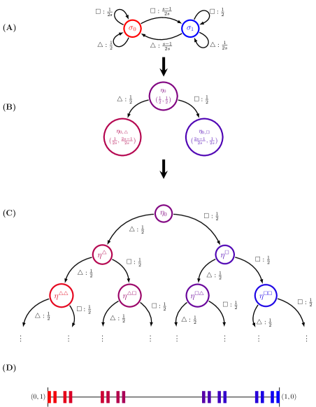
Figure 2: Constructing the mixed-state presentation of the $2$-state nonunifilar HMC shown in (A): The invariant state-distribution $\pi=(1/2,1/2)$. It becomes the first mixed state $\eta_{0}$ used in (B) to calculate the next set of mixed states—those having seen past words of length one. (C) In this example, infinitely-many mixed states are generated and $\bm{\mathcal{R}}$ is the middle-$1/s$ Cantor set. Color is used to indicate the relative closeness of each mixed state to the original states in (A). From $\eta_{0}$, one would need to see a word of infinite $\triangle$s to reach $\sigma_{0}$. In (D) the mixed states for $s=3$ are pictured on the $1$-simplex—the unit interval from $\eta=(0,1)$ to $\eta=(1,0)$. In this representation, the relationship to the Cantor set is visually clear.

III.1.1 Mixed-State Set

Assume we have an $N+1$-state HMC presentation $M$ with $k$ symbols ${x}\in\mathcal{A}$. For a length-$\ell$ word $w$ generated by $M$ let $\eta(w)=\Pr(\bm{\mathcal{S}}|w)$ be the observer’s belief distribution as to the process’ current state after observing $w$:

$$\eta(w)\equiv\Pr(\mathcal{S}_{\ell}|{X}_{0:\ell}=w,\mathcal{S}_{0}\sim\pi)~{}.$$ (5)

${X}\sim\eta$ means that random variable ${X}$ is distributed according to $\eta$.

The belief distributions $\eta(w)$ that an HMC can visit defines its set of mixed states:

$$\bm{\mathcal{R}}=\{\eta(w):w\in\mathcal{A}^{+},\Pr(w)>0\}~{},$$

where $\mathcal{A}^{+}$ indicates the set of all words with positive length. Generically, the mixed-state set $\bm{\mathcal{R}}$ for an $N$-state HMC is infinite, even for finite $N$ [14]. Figure 2 shows a case where the HMC generates the Cantor set as its mixed state set.

When observing a $N$-state machine, the vector $\bra{\eta(w)}$ lives in the (N-1)-simplex $\Delta^{N-1}$, the set such that:

$$\{\eta\in\mathbb{R}^{N}:\langle\eta\ket{{\mathbf{1}}}=1,\langle\eta\ket{\delta_{i}}\geq 0,i=1,\dots,N\}~{},$$

where $\bra{\delta_{i}}=\begin{pmatrix}0&0&\dots&1&\dots&0\end{pmatrix}$ and $\ket{{\mathbf{1}}}=\begin{pmatrix}1&1&\dots&1\end{pmatrix}$. We use this notation for components of the mixed-state vector $\eta$ to avoid confusion with temporal indexing.

III.1.2 Mixed-State Dynamic

The set of mixed states itself does not constitute a presentation. We must augment it with the state dynamic, which gives the transition probabilities between mixed states. Let the initial mixed state be the invariant probability $\pi$ over $M$’s states, so $\bra{\eta_{0}}=\bra{\pi}$. In the context of the mixed-state dynamic, mixed-state subscripts denote time. The probability of transitioning from $\bra{\eta(w)}$ to $\bra{\eta(w{x})}$ on observing symbol ${x}$ follows from Eq. 5 immediately; we have:

$$\Pr(\eta(w{x})|\eta(w))=\Pr({x}|\mathcal{S}_{\ell}\sim\eta(w))~{}.$$

This defines the mixed-state transition dynamic $\mathcal{W}$.

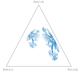
(a) Mixed state attractor for 3-state “alpha” machine.

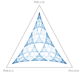
(b) Mixed state attractor for 3-state machine from Section VI, with $\alpha=0.6$ and $x=0.1$.

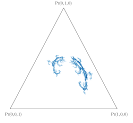
(c) Mixed state attractor for 3-state “beta” machine.

Figure 3: Simple HMCs generate MSPs with a wide variety of structures, many fractal in nature. Each subplot displays $10^{4}$ mixed states of a different, highly-nonunifilar $3$-state hidden Markov chain. The HMCs themselves are specified in Appendix A.

Given $M$’s symbol-labeled transition matrices, we can specify the mixed-state dynamic $\mathcal{W}$ in closed form. First, the probability of generating symbol ${x}$ when in mixed state $\eta$ is:

$$\Pr({x}|\eta)=\bra{\eta}T^{({x})}\ket{{\mathbf{1}}}~{},$$ (6)

where $T^{({x})}$ is the symbol-labeled transition matrix associated with the symbol ${x}$. Now, given a mixed state at time $t$, we may calculate the probability of seeing each ${x}\in\mathcal{A}$. Upon seeing symbol ${x}$, the current mixed state $\bra{\eta_{t}}$ is updated according to:

$$\bra{\eta_{t+1,{x}}}=\frac{\bra{\eta_{t}}T^{({x})}}{\bra{\eta_{t}}T^{({x})}\ket{{\mathbf{1}}}}~{}.$$ (7)

Equation (7) tells us that, by construction, the MSP is unifilar, since each possible output symbol uniquely determines the next (mixed) state. Taken together, Eqs. 6 and 7 define the mixed-state transition dynamic $\mathcal{W}$ as:

$$\Pr(\eta_{t+1},{x}|\eta_{t}) =\Pr({x}|\eta_{t})$$

$$=\bra{\eta_{t}}T^{({x})}\ket{{\mathbf{1}}}~{},$$

for all $\eta\in\bm{\mathcal{R}}$, ${x}\in\mathcal{A}$.

Together the mixed states and their dynamic define an HMC that is unifilar by construction. This is a process’ mixed-state presentation (MSP) $\mathcal{U}(\mathcal{P})=\{\bm{\mathcal{R}},\mathcal{W}\}$.

III.2 Constructing the Mixed-State Presentation

To explicitly find the MSP $\mathcal{U}=\{\bm{\mathcal{R}},\mathcal{W}\}$ for a given HMC $M$ we apply mixed-state construction:

1. Set $\mathcal{U}=\{\bm{\mathcal{R}}=\emptyset,\mathcal{W}=\emptyset\}$.

2. Calculate $M$’s invariant state distribution: $\pi=\pi T$.

3. Take $\eta_{0}$ to be $\bra{\pi}$ and add it to $\bm{\mathcal{R}}$.

4. For each current mixed state $\eta_{t}\in\bm{\mathcal{R}}$, use Eq. 6 to calculate $\Pr({x}|\eta_{t})$ for each ${x}\in\mathcal{A}$.

5. For $\eta_{t}\in\bm{\mathcal{R}}$, use Eq. 7 to find the updated mixed state $\eta_{t+1,{x}}$ for each ${x}\in\mathcal{A}$ with $\Pr({x}|\eta_{t})>0$.

6. Add $\eta_{t}$’s transitions to $\mathcal{W}$ and each $\eta_{t+1,x}$ to $\bm{\mathcal{R}}$.

7. For each new $\eta_{t+1}$, repeat steps 4-6 until no new mixed states are produced.

This algorithm need not terminate, as shown in Fig. 2, which depicts the MSP construction for the HMC in Fig. 1. However, it can terminate for HMCs described by finite-state $\epsilon$-machines. When working with HMCs for which the algorithm does not terminate, one must impose a limit on the number of generated mixed-states, effectively setting a level of approximation for $\bm{\mathcal{R}}$.

One may ask, given that mixed-state construction returns a unifilar HMC of the underlying process, is the MSP the same as the $\epsilon$-machine? It is not guaranteed to be so, as indeed is the case in Fig. 2. While the Cantor machine there generates an uncountably-infinite set of mixed states, the underlying process’ $\epsilon$-machine is a single-state fair coin—which has a one-state HMC as its $\epsilon$-machine. We see this by noting that the symbol-branching probabilities depicted in Fig. 2(C) are identical for every generated mixed state. This may seem a cause for concern. Perhaps we overestimated the necessary state size for the process in Fig. 2 by an infinite factor. However, this case is both rare and easy to check for, as discussed in Appendix B. By applying a simple check on the uniqueness of mixed states as they are constructed, we can confirm if the MSP is the underlying process’ $\epsilon$-machine. Unless otherwise noted, we take this to hold.

Although the most common purpose of applying mixed-state construction is to unifilarize an HMC, we may find the MSP of uHMCs as well. The MSPs of unifilar presentations are interesting and contain additional information beyond the initial unifilar presentation. For example, they typically contain transient causal states and these are employed to calculate many complexity measures that track convergence statistics [36]. The following only considers nontransient (asymptotically recurrent) mixed states.

The following also narrows the focus to mixed-state presentations of nonunifilar HMCs, which typically have an infinite mixed-state set $\bm{\mathcal{R}}$. By way of emphasizing a principle result—and Blackwell’s original point [14]—applying mixed-state construction even to nominally simple, finite-state, finite-alphabet nonunfilar HMCs results in an explosion of mixed states. Figure 3 gives three examples of MSPs with fractal mixed-state sets $\bm{\mathcal{R}}$, each generated by a three-state nonunifilar HMC.

III.3 MSP as an IFS

Specifying MSP construction in this way reveals that generating mixed states is a type of random dynamical system known as place-dependent iterated function system (IFS) [32]. For finite $k$ and space $\Delta$, place-dependent IFSs are characterized by a set of mapping functions:

$$\left\{f^{(x)}:\Delta\to\Delta~{}\middle|~{}x\in\{0,1\dots k\}\right\}~{},$$

and associated probability functions:

$$\left\{p^{(x)}:\Delta\to\left[0,1\right]~{}\middle|~{}x\in\{0,1\dots k\}\right\}~{}.$$

A place-dependent IFS generates a stochastic process over $\eta\in\Delta^{N}$ as follows: Given an initial position $\eta_{0}\in\Delta^{N}$, the probability distribution $\{p^{({x})}(\eta_{0}):{x}=1,\dots,k\}$ is sampled. According to the sample ${x}$, apply $f^{({x})}$ to map $\eta_{0}$ to the next position $\eta_{1}=f^{({x})}(\eta_{0})$. Resample $x$ from the distribution and continue, generating $\eta_{0},\eta_{1},\eta_{2},\ldots$.

An $N$-state HMC’s associated mixed-state presentation defines a place-dependent IFS over the $N-1$ simplex, with each symbol-labeled transition matrix $T^{(x)}$ defining a mapping function (Eq. 7) and associated probability function (Eq. 6). Our previous results showed that an IFS defined by an ergodic HMC generates an ergodic mixed-state process and has a unique attractor—the set of mixed states $\bm{\mathcal{R}}$ [32]. Additionally, this attractor has a unique, attracting, invariant measure known as the Blackwell measure $\mu_{B}(\bm{\mathcal{R}})$.

IV Structure of Infinite-State Processes

Our prior development showed how to use the MSP to find a process’ intrinsic randomness—in the form of Shannon entropy rate $h_{\mu}$ [32]. Our goal here is to complement the measure of randomness with a measure of structure.

Recall that for processes generated by finite unifilar HMCs a unique minimal presentation—the $\epsilon$-machine—exists. Due to the latter’s minimality, for such processes we can then define the statistical complexity $C_{\mu}$ using Eq. 4. In contrast, general (nonunifilar) HMCs have no such canonical minimal presentation. And so, the Shannon entropy of their presentation states is ambiguous. However, Section III demonstrated how to find the mixed-state presentation $\mathcal{U}(M)$ of a nonunifilar HMC $M$, which operation unifilarizes it. A heavy cost is levied—explosion of the mixed-state set. Nonetheless, using the MSP to develop a measure of structure for processes generated by HMCs is naturally appealing, since the MSP is unifilar and unique [32]. Indeed, in most cases, the MSP is the $\epsilon$-machine of the underlying process and so minimal (see Appendix B). And, when not, we can minimize the MSP by merging equivalent mixed states as we construct them.

However, the naive approach of simply measuring structure with statistical complexity $C_{\mu}$ introduces a problem: the statistical complexity diverges for an HMC with an uncountably-infinite state set $\bm{\mathcal{R}}$. In general, MSPs of HMCs are uncountably-infinite state, precluding distinguishing them via $C_{\mu}$. This being said, it is clear visually from Fig. 3 that HMCs with uncountably-infinite state spaces still have significant and distinct structures. We wish to find a way to measure and distinguish such structure. For this, we take inspiration from Shannon’s dimension rate [4] and call on a familiar tool.

Fractal dimension measures the rate at which a chosen size metric of a set diverges with the scale at which the set is observed [37, 38, 39, 40, 41]. Fractal dimension is also useful to probe the “size” of objects when cardinality is not informative. For example, the mixed-state presentation, generically, has an uncountable infinity of causal states. That observation is far too coarse, though, to distinguish the clearly distinct mixed-state sets $\bm{\mathcal{R}}$ in Fig. 3. Each is uncountably infinite, but the $\bm{\mathcal{R}}$’s geometries differ. Determining their fractal and other dimensions will allow us to distinguish them and allow us to introduce additional insights into the original process’ intrinsic information processing.

IV.1 Dimensions

Consider the mixed-state set $\bm{\mathcal{R}}$ on the simplex for an $N$-state HMC $M$ that generates a process $\mathcal{P}$. We consider two types of dimension for $\bm{\mathcal{R}}$: the Minkowski-Bouligand or box-counting dimension, often simply called the fractal dimension, and the information dimension.

To calculate the first, coarse-grain the $N$-simplex with evenly spaced subsimplex cells of side length $\epsilon$. Let $\mathcal{F}(\epsilon)$ be the set of cells that encompass at least one mixed state. Then $\bm{\mathcal{R}}$’s box-counting dimension is:

$$d_{0}(\bm{\mathcal{R}})=-\lim_{\epsilon\to 0}\frac{\log|\mathcal{F(\epsilon)}|}{\log\epsilon}~{},$$ (8)

where $|C|$ is the size of set $C$.

The information dimension tracks how the Blackwell measure $\mu_{B}(\bm{\mathcal{R}})$ scales with $\epsilon$. Let each cell in $\mathcal{F}(\epsilon)$ be a state and approximate the dynamic over $\mathcal{U}(M)$ by grouping all transitions to and from states encompassed by the same cell. This results in a finite-state Markov chain that generates an approximation of the original mixed-state process and has a stationary distribution $\mu(\mathcal{F}(\epsilon))$. Then $\mu_{B}(\bm{\mathcal{R}})$’s information dimension is:

$$d_{1}(\mu_{B}(\bm{\mathcal{R}})) =\lim_{\epsilon\to 0}\frac{H_{\mu}[\mathcal{F}(\epsilon)]}{\log\epsilon}~{},$$ (9)

where $H_{\mu}[\mathcal{F}(\epsilon)]=-\sum_{C_{i}\in\mathcal{F}(\epsilon)}\mu(C_{i})\log\mu(C_{i})$ is the Shannon entropy over the set $\mathcal{F}(\epsilon)$ of cells that cover attractor $\bm{\mathcal{R}}$ with respect to $\mu$.

IV.2 Dimensions and Scaling of HMCs

These dimensions give two complementary resource-scaling laws for HMC-generated processes. Rearranging Eq. 8, we see that the number of mixed states in our finite-state approximation to $\mathcal{U}(M)$ scales algebraically with $\bm{\mathcal{R}}$’s box-counting dimension:

$$|\mathcal{F}(\epsilon)|\sim\epsilon^{-d_{0}(\bm{\mathcal{R}})}~{}.$$ (10)

In other words, for an uncountably infinite MSP, the exponential growth rate of mixed states is $d_{0}(\bm{\mathcal{R}})$.

Similarly, the entropy of the Blackwell measure scales with the information dimension. Rearranging Eq. 9 shows that the state entropy of the finite-state approximation to $\mathcal{U}(M)$ scales logarithmically with $\bm{\mathcal{R}}$’s information dimension with respect to the Blackwell measure:

$$H_{\mu}[\mathcal{F}]\sim d_{1}(\mu_{B})\cdot\log\epsilon~{}.$$ (11)

As $\epsilon\to 0$, $|\mathcal{F}|$ and $H_{\mu}(\mathcal{F})$ diverge and $d_{0}$ and $d_{1}$ are the divergence rates, respectively. The remainder focuses on $d_{1}$ as applied to the $\epsilon$-machine, for which it describes the rate of divergence of statistical complexity $C_{\mu}$.

V Statistical Complexity Dimension

We refer to the information dimension $d_{1}(\mu)$ of the $\epsilon$-machine the statistical complexity dimension $d_{\mu}$.

Applying $d_{1}$ to the Blackwell measure $\mu_{B}(\bm{\mathcal{R}})$ gives the rate of divergence of $C_{\mu}$ as one constructs increasingly better finite-state approximations to the infinite-state $\epsilon$-machine. In this way, $d_{\mu}$ describes the divergence of memory resources when attempting to optimally predict a process that requires an uncountably-infinite number of predictive features. This is a unique, minimal description of the process’ structural complexity. This solves the challenge posed in the introduction: quantifying structure for a broad class of truly complex systems.

When a process may be optimally predicted with a finite number of predictive features, the statistical complexity dimension vanishes. In this case, the more relevant complexity measure is the original $\epsilon$-machine statistical complexity $C_{\mu}$, which is is finite. When a process requires uncountably-infinite causal states, but may be generated with a minimal $N$-state (nonunifilar) HMC, the statistical complexity is less than or equal to $N-1$. This is the associated IFS’s embedding dimension, since the mixed states lie in a space of dimension $N-1$.

Unfortunately, directly calculating the information dimension using Eq. 9—and therefore calculating the statistical complexity dimension $d_{\mu}$—is nontrivial, as it requires estimating a fractal measure. Fortunately, to calculate the $d_{\mu}$ of the mixed state attractor $\bm{\mathcal{R}}$, we can leverage the associated generating dynamical system (see Section III.3).

V.1 Dimension from Dynamical (In)Stabilities

We can link the information dimension of an MSP’s mixed state set $\bm{\mathcal{R}}$ to the stability properties of the associated IFS. This starts with determining the local time-average stability and instability of orbits within an attractor via the spectrum of Lyapunov characteristic exponents $\Gamma=\{\lambda_{1},\ldots,\lambda_{N}:\lambda_{i}\geq\lambda_{i+1}\}$ [42, 43]. Individual LCEs $\lambda_{i}$ measure the average local growth or decay rate of orbit perturbations. The net result is a list of quantities that indicate long-term orbit instability ($\lambda_{i}>0)$ and orbit stability ($\lambda_{i}<0)$ in complementary directions. Usefully, their sum gives the net state-space divergence—volume loss for dissipative systems. The sum of the positive LCEs is the dynamical system’s entropy rate [44, 45, 46, 42, 41]—the net information generation.

To motivate our present use of the Lyapunov spectrum, it will help to develop a simple intuition for how the LCEs relate to dimension. Both of our previously defined dimensional quantities—Eq. 9 and Eq. 8—depended on the growth rate of cells needed to cover the attractor as we take the side length of the cells to zero. First, imagine the attractor of a two-dimensional map with LCEs $\lambda_{1}>0>\lambda_{2}$ and whose state space is covered with equally spaced squares of side length $\epsilon$. After iterating the map $q$ times, for $\epsilon$ small enough, the local action of the map is approximately linear. From the LCE definition, this means it takes the initial square cells to rectangles of average length $(e^{\lambda_{1}q})\epsilon$ and average width $(e^{\lambda_{2}q})\epsilon$. Now, consider covering the attractor with a new set of squares of side length $(e^{\lambda_{2}q})\epsilon$. We can see by inspection that this requires roughly $e^{\left(\lambda_{1}/\lambda_{2}\right)q}$ squares per rectangle. In this way, the Lyapunov exponents relate to the scalings measured by dimension quantities [47].

Indeed, this relationship has resulted in the definition of a Lyapunov dimension $d_{\Gamma}$ in terms of the spectrum $\Gamma$ [48]:

$$d_{\Gamma}=\left\{\begin{aligned} &k+\frac{\sum_{i}^{k}\lambda_{i}}{|\lambda_{k+1}|}~{},&\sum_{i}^{N}\lambda_{i}<0\\ &N~{},&\sum_{i}^{N}\lambda_{i}\geq 0\end{aligned}\right.~{},$$ (12)

where $k$ is the largest index such that the summation $\sum_{i}^{k}\lambda_{i}$ remains positive. If $\lambda_{1}<0$, $d_{\Gamma}=0$. Its name helps distinguish the conditions under which the relationships between the various dimensions actually hold. (There are many conditions and system classes that this summary necessarily leaves out.)

It has been shown that for any ergodic, invariant probability measure $\mu$:

$$d_{1}(\mu)\leq d_{\Gamma}~{},$$

with equality when $\mu$ is a Sinai-Bowen-Ruelle (SBR) measure [49]. Furthermore, it was conjectured that for “typical dynamical systems”, the Lyapunov dimension $d_{\Gamma}$ equals the information dimension $d_{1}$ [48]. This remarkable relationship directly relates a system’s dynamics to the geometry and natural measure of its attractor. Additionally, and usefully, Eq. 12 gives us a tractable method to find the information dimension of an attractor generated by a dynamical system when the equality holds and an upper bound when it does not.

Figure 4: Overlap problem on the $1$-simplex $\Delta^{1}$: Two distinct IFSs are considered, each with two mapping functions. The images of the mapping functions over the entire simplex are depicted in red and blue. (A) Images of the mapping functions $f^{(0)}$ and $f^{(1)}$ do not overlap—every mixed state $\eta_{t}\in\bm{\mathcal{R}}$ has a unique pre-image. (B) Images of the mapping functions overlap (purple Overlapping Region)—there exist $\eta_{1},\eta_{2}\in\bm{\mathcal{R}}$ such that $f^{{}^{\prime}(0)}(\eta_{1})=f^{{}^{\prime}(1)}(\eta_{2})=\eta_{3}$. This case is an overlapping IFS.

V.2 Calculating Statistical Complexity Dimension

We now have in hand two important pieces. First, the definition of statistical complexity dimension $d_{\mu}$ as the information dimension of an $\epsilon$-machine. Second, we have a bound on the information dimension of an attractor, given knowledge of the generating system’s dynamics. To complete our picture, we now address the final puzzle piece.

As Section V.1 discussed, there is a direct relationship between the information dimension of a chaotic attractor and the dynamics of the system to which the attractor belongs. Furthermore, as discussed in Section III.3, every HMC has an associated random dynamical system—the iterated function system (IFS)—which has the HMC’s set of mixed states $\bm{\mathcal{R}}$ as its unique attractor. Combining these two facts allows us to exactly calculate $d_{\mu}$ in many cases of interest.

An advantage of working with IFSs defined by HMCs is a clean division exhibited by their Lyapunov spectrum. It has been shown that the entropy rate of the generated process is equivalent to the largest Lyapunov exponent [50, 51]. Calculating this was the main topic of the prequel to the present work [32]. Furthermore, due to the contractivity of the IFS mapping functions, all other Lyapunov exponents will necessarily be negative. For a review of calculating the Lyapunov exponents for IFSs, see Appendix E.

Therefore, the Lyapunov dimension of an IFS is:

$$\widetilde{d_{\Gamma}}=\left\{\begin{aligned} &k-1+\frac{h_{\mu}+\sum_{i}^{k-1}\lambda_{i}}{|\lambda_{k}|},&h_{\mu}+\sum_{i}^{N}\lambda_{i}<0\\ &N~{},&h_{\mu}+\sum_{i}^{N}\lambda_{i}\geq 0\end{aligned}\right.,$$ (13)

where $k$ is now the largest index for which $h_{\mu}+\sum_{i}^{k}\lambda_{i}>0$. This is simply Eq. 12, as if $h_{\mu}$ was the largest Lyapunov exponent.

Under specific technical conditions to be discussed shortly, the IFS $d_{\Gamma}$ is exactly equal to the information dimension of the IFS’s attractor and, therefore, is $d_{\mu}$ [52]. In general, relaxing those conditions, $\widetilde{d_{\Gamma}}$ upper bounds the statistical complexity dimension:

$$\widetilde{d_{\Gamma}}\geq d_{\mu}~{}.$$ (14)

Assembling these pieces together determines the basic algorithm to calculate (or bound) the statistical complexity dimension:

1. For an $N$-state HMC $M$ with $|\mathcal{A}|=k$, write down the associated IFS with $k$ symbol-labeled mapping functions and probability functions.

2. Calculate the entropy rate $h_{\mu}$ using the Blackwell limit (see [32]).

3. Calculate the negative Lyapunov exponents $\left\{\lambda_{1},\dots,\lambda_{N-1}\right\}$ (see Appendix E).

4. Compute the Lyapunov dimension $d_{\Gamma}$ using Eq. 13.

As mentioned, in specific cases, the Lyapunov dimension is exactly equal to the statistical complexity dimension, and our task is complete. However, there are major technical concerns with when we have only the bound in Eq. 14 and with its tightness then.

V.3 The Overlap Problem

A subtle disadvantage of working with IFSs is a direct result of the stochastic nature of them as random dynamical systems. We must consider the overlap problem, which concerns the ranges of the symbol-labeled mapping functions $f^{(i)}$, illustrated in Fig. 4. Specifically, the problem means that we must distinguish between IFSs that meet the open set condition and those that do not.

Definition 6.

An iterated function system with mapping functions $f^{(\eta)}:\Delta^{N}\to\Delta^{N}$ satisfies the open set condition (OSC) if there exists an open set $U\in\Delta^{N}$ such that for all $\eta,\zeta\in\Delta^{N}$:

$$f^{\eta}(U)\cap f^{\zeta}(U)=\emptyset,\>\>\>\>\eta\neq\zeta~{}.$$

IFSs that meet the OSC are nonoverlapping IFSs.

When the images of the symbol-labeled mappings overlap the inequality in Eq. 14 is strict. To briefly outline the consequences, for an overlapping IFS the entropy rate $h_{\mu}$ does not accurately capture state-space expansion. And, this causes the IFS $d_{\Gamma}$ (Eq. 13) to overestimate the information dimension. As a rule of thumb, the degree to which the mappings overlap determines the magnitude of the bound’s error. The impact of overlaps is significant. It is explored both in Section VI, where we calculate the statistical complexity dimension for HMCs with and without overlap, as well as in the sequel, which diagnoses the problem’s origins and provides an algorithmic solution.

For now, to give a workable approach, we simply introduce two extra steps to the $d_{\mu}$ algorithm from the previous section:

1. Determine if the Open Set Condition is met using the mapping functions $f^{(i)}$.

2. If the OSC is not met, estimate the degree of overlap to determine the closeness of the bound on $d_{\mu}$.

V.4 Statistical Complexity Dimension for Processes Generated by Two-State HMCs

Finally, we analyze two-state HMCs, for which Eq. 13 simplifies significantly. When there is no overlap in the maps, we have exact results for $d_{\mu}$.

Figure 5: Mixed-state attractors generated by a $3$-state HMC parametrized over $\alpha\in[0,1]$ and $x\in[0,0.5]$. The HMC itself is given in Section VI. $10^{5}$ mixed states are plotted for each attractor, with the initial $5\times 10^{4}$ states thrown away as transients. The ranges of the symbol-labeled maps are color shaded, revealing regions of their image overlap on the attractor. Comparing to Section VI, the red, blue, and green regions represent the images of the mapping functions defined by $T^{\square}$, $T^{\triangle}$, and $T^{\circ}$, respectively.

For two-state nonunifilar HMCs, the mixed-state set lives on the $1$-simplex $\Delta^{1}$—the unit interval from $\eta=(0,1)$ to $\eta=(1,0)$. Mixed states $\eta\in\bm{\mathcal{R}}$ and the dynamic on them exist in a one-dimensional space and, thus, there is a single negative Lyapunov exponent $\lambda_{1}<0$.

In this case, the calculation of the negative Lyapunov exponent is particularly direct, since the maps are all one-dimensional. The negative Lyapunov exponent for a one-dimensional map $\eta_{n+1}=f(\eta_{n})$ is:

$$\lambda(\eta_{0})=\lim_{N\to\infty}\frac{1}{N}\sum_{i=0}^{N-1}\log\left|\frac{df(\eta_{i})}{d\eta}\right|$$

for an orbit starting at $\eta_{0}$. For an IFS with a set of of mapping functions $\{f^{({x})}\}$, we find $\lambda$ as the weighted average of the Lyapunov exponents of each map:

$$\lambda_{\mu}=\int\sum_{{x}}p^{({x})}(\eta)\log\left|\frac{df^{({x})}(\eta)}{d\eta}\right|d\mu~{},$$

where $\mu$ is the IFS’s Blackwell measure. We can apply ergodicity to transform this into a summation over time for ease of calculation.

If a two-state HMC has an MSP with an uncountable infinity of mixed states and its corresponding IFS satisfies OSC, there is a simple relationship between the entropy rate, the Lyapunov exponent, and the statistical complexity dimension. This is given by:

$$d_{\mu}(\mu)=-\frac{h_{\mu}}{\lambda_{\mu}}~{},$$ (15)

recalling that $h_{\mu}>0$, so that the dimension is always positive. Failing OSC, this ratio is an upper bound on the dimension of the measure $\mu$ [53]. For a discussion of the intuition behind this formula, see Appendix C.

(a) Mixed-state attractor area estimated across $\alpha$ and $x$. The area is minimized along lines of $\alpha=1/3$ and $x=1/3$, where the attractor becomes point-like.

(b) Mixed-state attractor Lyapunov dimension does not detect the collapse to zero dimension along $\alpha=1/3$, which is due to overlaps.

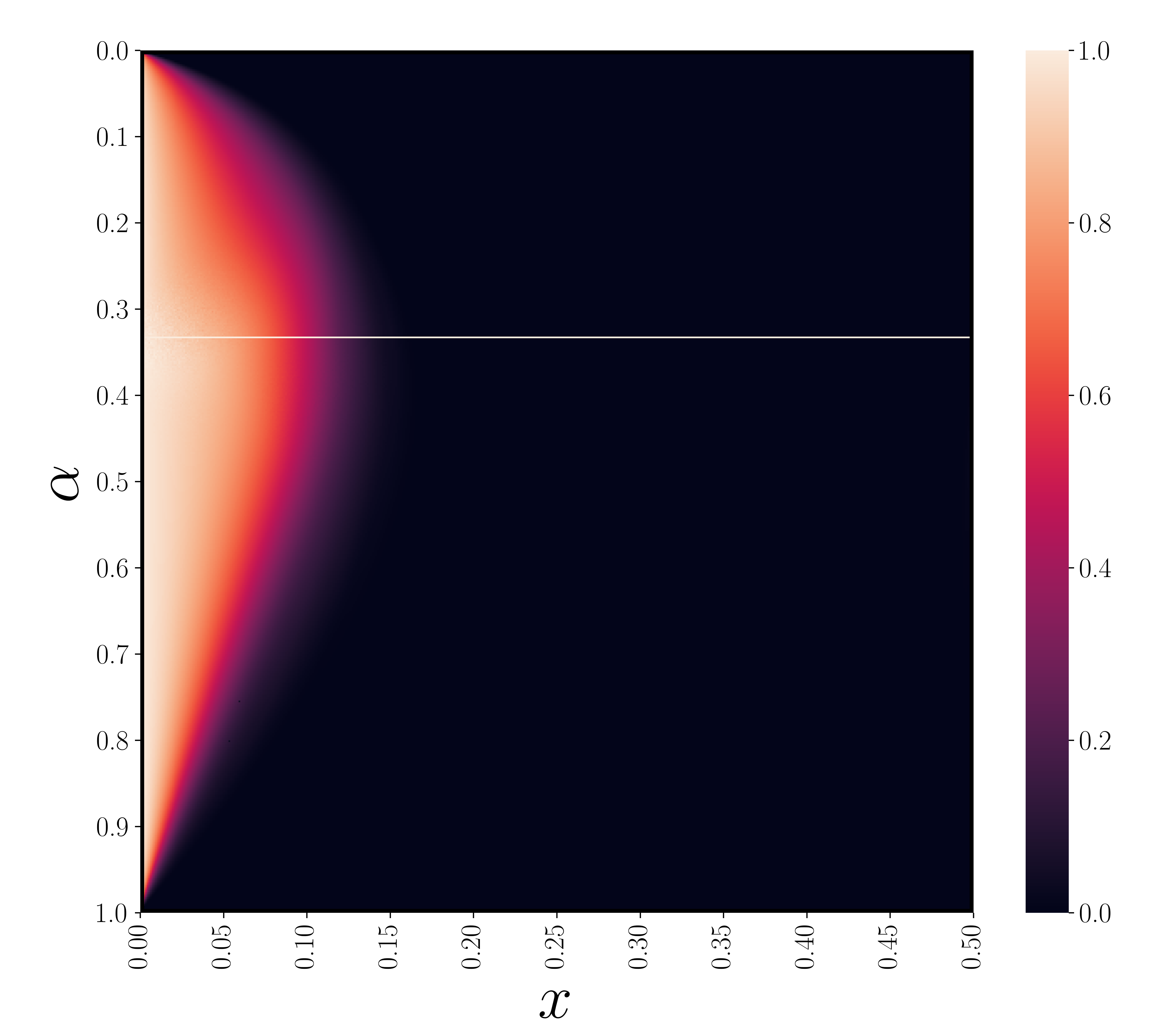
(c) Percentage of attractor area in which there is overlap.

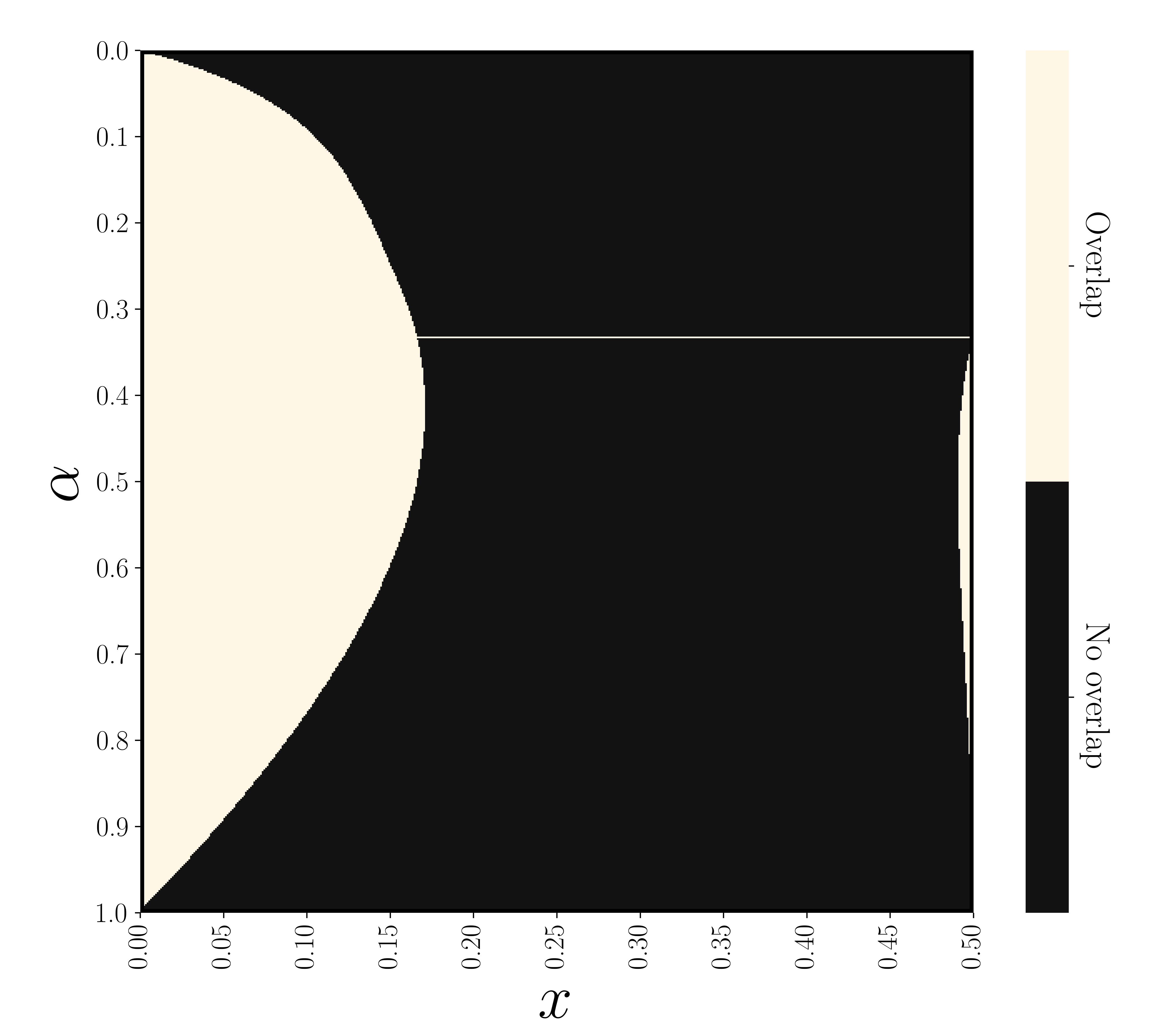
(d) Overlap in the attractor area. Comparing with (c), for much of this area, the overlap is very small.

Figure 6: Attractor area, overlap regions, and Lyapunov dimension of the mixed-state attractors shown in Fig. 5, parametrized by $\alpha=[0,1]$ and $x=[0,0.5]$. The HMC itself is given in Section VI. See Appendix E and Appendix F for a detailed discussion of the production of these plots.

VI Multi-state HMC Examples

Notably, the Lyapunov dimension Eq. 15 for more-than-two-state HMCs is easily shown to be correct when the maps are similitudes and the probability functions are constant. The latter is seen, for example, with the Sierpinski triangle, as discussed in Appendix D.

However, we are generally interested in multi-state HMCs that do not produce perfectly self-similar fractals. Furthermore, we are often interested in considering physical systems described by parametrized HMCs, such as those that arose in the two prequels on quantum measurement processes and information engine functionality [33, 18]. In such cases, an HMC determined by an application may meet the OSC in some regions of parameter space and fail to do so in others. Let’s consider an HMC that spans the breadth of these possible behaviors, from zero overlap to complete overlap. This will demonstrate the range of applicability of our statistical complexity dimension algorithm. And, ultimately in a sequel [54], it leads to a practical algorithm and a conjecture for general HMCs.

Consider the following HMC with $3$ symbols and $3$ states:

$$T^{\square} =\begin{pmatrix}\alpha y&\beta x&\beta x\\ \alpha x&\beta y&\beta x\\ \alpha x&\beta x&\beta y\end{pmatrix},~{}T^{\triangle}=\begin{pmatrix}\beta y&\alpha x&\beta x\\ \beta x&\alpha y&\beta x\\ \beta x&\alpha x&\beta y\end{pmatrix},~{}\text{and}$$

$$T^{\circ} =\begin{pmatrix}\beta y&\beta x&\alpha x\\ \beta x&\beta y&\alpha x\\ \beta x&\beta x&\alpha y\end{pmatrix}~{},$$ (16)

with $\beta=(1-\alpha)/2$ and $y=1-2x$. By inspection, we see that $\alpha$ takes on any value from $0$ to $1$ and $x$ may range from $0$ to $1/2$.

Figure 5 shows how the MSP attractors change across the $(\alpha,x)$ parameter space. Each black dot is a generated mixed state, while the colored regions show the range of each symbol-labeled map.

For example, on one hand, in the top left corner with $\alpha=0.01$ and $x=0.01$, we find an attractor that fills the simplex, with moderate amounts of overlap. On the other, $\alpha=0.79$ and $x=0.11$ produces an attractor with no overlap, and clearly defined regions.

Moreover, for any $\alpha$, choosing $x=1/3$ leads the MSP attractor to collapse to a finite $3$-state HMC, since the symbol-labeled mapping functions become constant functions. In this case, there is no overlap, as each symbol-labeled map takes on a different constant value.

However, when $\alpha=\beta=1/3$, all symbol-labeled mapping functions are identical. Therefore, the attractor is the single fixed-point shared by all three maps—a single-state HMC. This is a case of maximal possible overlap. Along both lines in parameter space the MSP collapses to a finite-state HMC, so $d_{\mu}=0$, by definition. However, these different mechanisms of state-collapse are relevant in calculation of $d_{\Gamma}$ via Eq. 13.

First, consider Fig. 6a, which illustrates the estimated area on the simplex taken up by the attractor across parameter space. For a discussion of how attractor area was estimated, see Appendix F. This figure matches the grid in Fig. 5: lower values of $x$ produce larger attractors, excepting the region near $\alpha=1/3$, where the area drops to zero.

Now, the area taken up by an attractor is not a good proxy for dimension—we may have very small-in-size attractors with large dimension. Indeed, this is the case for most values of $\alpha$ near $1/3$, where the attractors are very small but whose $d_{\mu}\to 2$. However, we know from analyzing the attractor grid that for HMCs lying exactly on this line, the attractor is instantaneously finite state. And so, the statistical complexity dimension $d_{\mu}$ must discontinuously drop to zero. However, this is not accurately reflected by $d_{\Gamma}$, as seen in Fig. 6b.

That said, $d_{\Gamma}$ clearly smoothly approaches zero as $x\to 1/3$. Along the vertical line, $d_{\Gamma}$ is correctly exactly zero. This is the other line in parameter space where the MSP is finite state and $d_{\mu}$ is analytically known to be zero. The disparity, in both correctness and continuity, is due to the different mechanisms driving the collapse noted above.

As $x\to 1/3$, the slopes of the symbol-labeled mapping functions approach zero. When $x=1/3$, the symbol-labeled mapping functions become constant values, as reflected in the Lyapunov exponents and consequently in $d_{\Gamma}$. The constant functions have negative Lyapunov exponents of negative infinity, sending Eq. 13 to zero.

In contrast, along the $\alpha=1/3$ line, the contraction in the state space is a result of the maps instantaneously sharing a fixed point. For $\alpha=1/3\pm\epsilon$, the attractor is not finite. In this region of parameter space, symbol-labeled maps are not infinitely contracting, so $d_{\Gamma}$ badly overestimates $d_{\mu}$ along the $\alpha=1/3$ line. This illustrates the importance of the OSC on the bound.

This poses the question, which regions in HMC parameter space exhibit overlap IFS maps? Figure 6d depicts parameter space regions in terms of overlap or no overlap. Figure 6c shows this as a percentage of the total attractor area. For a discussion of how overlap was determined, please see Appendix F. Comparing the two, we see that there is a significant region over which overlap does exist for $x<0.15$ and a smaller region where $x>0.48$. However, for much of that region the attractor’s overlap area is relatively small. As a rule of thumb, the gap between $d_{\Gamma}$ and $d_{\mu}$ for the mixed-state set is determined by the percentage of the attractor that is affected by overlap. If the overlap region is relatively small, in comparison to the size of the attractor, $d_{\Gamma}$ may be very close to $d_{\mu}$.

However, if the overlap is very large, $d_{\Gamma}$ may be a dramatic overestimation of $d_{\mu}$. This occurs when $\alpha=1/3$ and $x<0.15$. The statistical complexity dimension $d_{\mu}$ vanishes, yet the Lyapunov dimension saturates at $d_{\Gamma}=2.0$.

We also note that the mechanism driving the collapse of the MSP attractor at $\alpha=1/3$ is a discontinuity in the parameter space, as compared to $x=1/3$. This is because state space collapse due to overlap requires the maps to be identical, and even minute differences in the symbol-labeled transition matrices will produce an uncountably-infinite MSP, potentially with $d_{\mu}=2.0$. This encourages us to consider not just the statistical complexity dimension, but also the area of the attractor and the nearby regions in parameter space for a clearer understanding of the underlying HMC. In this, the tools developed here, by allowing (computationally-efficient) surveys of large regions of parameter space, are particularly useful.

Thus, while there are wide parameter regions in which the analysis developed here is correct and efficient, this is not the entire story. Overlap must be addressed for full generality. Our sequel shows how to correct for overestimating statistical complexity dimension, allowing accurate calculation across the entire parameter space [54]. However, the exploratory observations outlined here are a crucial diagnostic guide to those further developments.

VII Conclusion

Our development opened by considering the challenge of quantifying the structure of complex systems. For well over a half a century, since Kolmogorov and Sinai introduced Shannon’s mathematical theory of communication to dynamical systems, the entropy rate stood as the standard by which to quantify randomness in time series and in chaotic dynamical systems. Quantifying observable patterns remained a more elusive goal. However, with developments from computational mechanics, it has become possible to answer questions of structure and pattern, at least for stochastic processes generated by finite-state predictive machines, including the symbolic dynamics generated by chaotic dynamical systems.

To handle processes generated by finite-state nonpredictive (nonunifilar) hidden Markov chains, we developed the mixed-state presentation. This unifilarizes general HMCs, giving a predictive presentation that itself generates the process. However, adopting a unifilar presentation came at a heavy cost: Generically, they are infinite state and so previous structural measures diverge. Nonetheless, we showed how to work constructively with these infinite mixed-state presentations. In particular, we showed that they fall into a common class of dynamical system: The mixed-state presentation is a place-dependent iterated function system. Due to this, a number of results from dynamical systems theory can be applied to more fully describe the original stochastic process.

Previously, others considered the IFS-HMC connection [55, 56]. Complementing those efforts, we expanded the role of the mixed-state presentation to calculate entropy rate and demonstrated its usefulness in determining the underlying structural properties of the generated process. Indeed, Fig. 3 and Fig. 5 show how visually striking—and distinct—mixed-state sets generated by HMCs are.

Here, moving in a new direction beyond previous efforts, we established that the information dimension of the mixed-state attractor is exactly the divergence rate of the statistical complexity [57]—a measure of a process’ structural complexity that tracks memory. Thus, processes in this class effectively increase their use of memory, “creating” mixed or causal states, on the fly. Furthermore, we introduced a method to calculate the information dimension of the mixed-state attractor from the Lyapunov spectrum of the mixed-state IFS. In this way, we demonstrated that coarse-graining the mixed-state simplex—the previous method for studying the structure of infinite-state processes [58]—can be avoided altogether. This greatly improves accuracy and computational speed and deepens our understanding of the origins of complexity in stochastic processes.

During the development, we noted several obstacles. Most importantly, the presence of overlap and failure to meet the Open Set Condition causes the Lyapunov dimension to be a strict upper bound, and some times quite a poor one, on the statistical complexity dimension. The final work of our trilogy [54] introduces a measure of how badly the entropy rate overestimates the expansion of the mixed-state set. Combining this measure with the Lyapunov-information dimension conjecture finally yields a correct Eq. 13 to apply to HMCs with overlap; that is, for processes generated by all general HMCs.

To close, we note that the structural tools introduced here and the entropy-rate method introduced previously have been put to practical use in two previous works. One diagnosed the origin of randomness and structural complexity in quantum measurement [33]. The other exactly determined the thermodynamic functioning of Maxwellian information engines [18], when there had been no previous method for this kind of detailed and accurate analysis. At this point, however, we leave the full explication of these techniques and further analysis on how mixed states reveal the underlying structure of processes generated by hidden Markov chains to the sequel [54].

Supplementary Materials
Divergent Predictive States:
The Statistical Complexity Dimension of
Stationary, Ergodic Hidden Markov Processes
Alexandra Jurgens and James P. Crutchfield
arXiv:2102.10487

The Supplementary Materials give the HMCs for the example processes considered, review MSP minimality, draw a correspondence with the Baker’s Map on the unit square, layout an HMC whose mixed-state set $\bm{\mathcal{R}}$ is the well-known Sierpinski Triangle fractal, and review Lyapunov characteristic exponents and calculating their spectrum for IFSs.

Appendix A Nonunifilar HMC Examples

We reproduce here the HMCs used to create Fig. 3. First, the “alpha” HMC, from Fig. 3a, is given by::

$$T^{\square} =\begin{pmatrix}2.734\times 10^{-2}&0.392&1.924\times 10^{-2}\\ 0.475&2.176\times 10^{-2}&2.766\times 10^{-4}\\ 0.224&2.711\times 10^{-3}&0.236\end{pmatrix},$$ (S1)

$$T^{\triangle} =\begin{pmatrix}1.845\times 10^{-3}&0.133&0.259\\ 3.913\times 10^{-2}&0.315&2.789\times 10^{-2}\\ 0.467&1.015\times 10^{-2}&4.699\times 10^{-3}\end{pmatrix},~{}\text{and}~{}$$

$$T^{\circ} =\begin{pmatrix}9.782\times 10^{-2}&3.374\times 10^{-2}&3.644\times 10^{-2}\\ 5.422\times 10^{-2}&6.503\times 10^{-2}&2.090\times 10^{-3}\\ 5.328\times 10^{-2}&1.278\times 10^{-3}&8.778\times 10^{-4}\end{pmatrix}~{},$$

Fig. 3b is given by Section VI, at $\alpha=0.6$ and $x=0.1$. The “beta” HMC, in Fig. 3c, is given by:

$$T^{\square} =\begin{pmatrix}5.001\times 10^{-2}&0.388&4.251\times 10^{-2}\\ 0.464&4.484\times 10^{-2}&2.495\times 10^{-2}\\ 0.232&2.720\times 10^{-2}&0.243\end{pmatrix},$$ (S2)

$$T^{\triangle} =\begin{pmatrix}1.708\times 10^{-3}&0.123&0.240\\ 3.623\times 10^{-2}&0.292&2.583\times 10^{-2}\\ 0.432&9.397\times 10^{-3}&4.351\times 10^{-3}\end{pmatrix},~{}\text{and}~{}$$

$$T^{\circ} =\begin{pmatrix}9.0576\times 10^{-2}&3.124\times 10^{-2}&3.374\times 10^{-2}\\ 5.020\times 10^{-2}&6.021\times 10^{-2}&1.935\times 10^{-3}\\ 4.933\times 10^{-2}&1.183\times 10^{-3}&8.127\times 10^{-4}\end{pmatrix}~{},$$

Due to finite numerical accuracy, reproduction of the attractors using these specifications may differ slightly from Fig. 3.

Appendix B Mixed-State Presentation Minimality

Given an HMC $M$, minimality of infinite-state mixed-state presentations $\mathcal{U}(M)$ is an open question. MSPs are not guaranteed to be minimal. In fact, it is possible to construct MSPs with an uncountably-infinite number of states for a process that requires only one state to optimally predict, as seen with the Cantor machine process in Figs. 1 and 2. Note that while this HMC generates an uncountable number of mixed states, each one has the same emitted-symbol probability distribution, indicating that all states can be merged into a single state with no loss of predictability. Indeed, the $\epsilon$-machine for the HMC depicted in Fig. 1 is simply the single-state Fair Coin HMC.

A proposed solution to this needless presentation verbosity is a short and simple check on mergeablility of mixed states. This refers to any two distinct mixed states that have the same conditional probability distribution over future strings; i.e., any two mixed states $\eta_{0}$ and $\zeta_{0}$ for which:

$$\Pr({X}_{0:L}|\eta_{0})=\Pr({X}_{0:L}|\zeta_{0})~{},$$ (S3)

for all $L\in\mathbb{N}^{+}$.

A benefit of the IFS formalization of the MSP is the ability to directly check for duplicated states and therefore determine if the MSP is nonminimal. We check this by considering, for an $N+1$ state HMC $M$ with alphabet $\mathcal{A}=\{0,1,\dots,k\}$, the dynamic not only over mixed states, but probability distributions over symbols. Let:

$$P(\eta)=\left(p^{(0)}(\eta),\dots,p^{(k-1)}(\eta)\right)$$ (S4)

and consider Fig. S1. For each mixed state $\eta\in\Delta^{N}$, Eq. S4 gives the corresponding probability distribution $\rho(\eta)\in\Delta^{k}$ over the symbols ${x}\in\mathcal{A}$. Let $M$ emit symbol ${x}$, then the dynamic from one such probability distribution $\rho\in\Delta^{k}$ to the next is given by:

$$g^{({x})}(\rho_{t}) =P\circ f^{({x})}\circ P^{-1}(\rho)$$

$$=\rho_{t+1,{x}}~{}.$$ (S5)

From this, we see that if Eq. S5 is invertible, $g^{({x})}:\Delta^{k}\to\Delta^{k}$ is well defined and has the same functional properties as $f^{({x})}$. In other words, in this case, it is not possible to have two distinct mixed states $\eta,\zeta\in\Delta^{N}$ with the same probability distribution over symbols. And, the probability distributions can only converge under the action of $g^{({x})}$ if the mixed states also converge under the action of $f^{({x})}$. When every mixed state has a unique outgoing probability distribution, these states are also the causal states, and the MSP is the process’ $\epsilon$-machine. Our companion work [59] elaborates on this and the implications for identifying the embedding dimension of minimal generators.

Figure S1: Commuting diagram for probability functions $P=\{p^{(x)}\}$, mixed-state mapping functions $f^{(x)}$, and proposed symbol-distribution mapping functions $g^{(x)}$.

Appendix C Correspondence with Baker’s Map

The simple dimension formula in Eq. 15 may not seem easily motivated. Especially, considering that, in general, both positive and negative Lyapunov exponents are required to have a nontrivial attractor. However, for iterated function systems, all Lyapunov exponents are negative and the expansive role played by positive Lyapunov exponents is instead played by an IFS’s stochastic map selection, as measured by the entropy rate $h_{\mu}$.

This is more intuitively appreciated by comparing the two-state IFS with the Baker’s map. Consider the Baker’s map:

$$x_{n+1} =\left\{\begin{aligned} &\frac{x_{n}}{s_{0}}~{},&y<p\\ &\frac{x_{n}+s_{1}-1}{s_{1}}~{},&y\geq p\end{aligned}\right.\text{~{}~{}~{}and}$$

$$y_{n+1} =\left\{\begin{aligned} &\frac{y_{n}}{p}~{},&y<p\\ &\frac{y_{n}-p}{p-1}~{},&y\geq p\end{aligned}\right.$$

It has LCE spectrum $\Lambda=\{\lambda_{1},\lambda_{2}\}$, where:

$$\lambda_{1} =p\log(p)+(1-p)\log(1-p)$$

$$\lambda_{2} =p\log(1/s_{0})+(1-p)\log(1/s_{1})~{}.$$

Note that $\lambda_{1}>0$ and $\lambda_{2}<0$. Then, the Lyapunov dimension is:

$$d_{\Gamma}=1-\frac{\lambda_{1}}{\lambda_{2}}~{}.$$

To compare this to an IFS, take:

$$\{f(x)\} =\left\{\frac{x_{n}}{s_{0}},\frac{x_{n}+s_{1}-1}{s_{1}}\right\}~{}\text{and}$$

$$\{p(x)\} =\{p,1-p\}~{}.$$

Thus, we identify the $y$ coordinate as controlling the stochastic map choice. The dynamic over position in the $y$ direction exactly determines the IFS entropy rate. Since the Baker’s map is volume preserving in $y$, the extra dimension always contributes a plus one in the dimension formula. In other words, the dimension along a slice of constant $y$ equals the IFS dimension.

Appendix D Sierpinski’s Triangle

The Sierpinski triangle is a canonical Cantor set in two dimensions. An HMC that generates a MSP attractor that is the Sierpinski triangle is:

$$T^{(0)} =\begin{pmatrix}a&0&a(s-1)\\ 0&a&a(s-1)\\ 0&0&as\end{pmatrix},~{}T^{(1)}=\begin{pmatrix}\frac{1-as}{2}&0&0\\ \frac{(1-as)(s-1)}{2s}&\frac{1-as}{2s}&0\\ \frac{(1-as)(s-1)}{2s}&0&\frac{1-as}{2s}\end{pmatrix},~{}\text{and}~{}T^{(2)}=\begin{pmatrix}\frac{1-as}{2s}&\frac{(1-as)(s-1)}{2s}&0\\ 0&\frac{1-as}{2}&0\\ 0&\frac{(1-as)(s-1)}{2s}&\frac{(1-as)(s-1)}{2s}\end{pmatrix}~{},$$ (S6)

where $s$ controls the contraction coefficient and $a$ controls the probability of selecting the maps. This HMC produces constant probability functions:

$$p^{(0)} =as~{},~{}p^{(1)}=\frac{1-as}{2}~{},~{}\text{and}~{}p^{(2)}=\frac{1-as}{2}~{}.$$

and, therefore, linear mappings, since $f^{(0)}=\bra{\eta}T^{(i)}/p^{(i)}(\eta)$. The constant probability functions make the entropy rate trivial to calculate. And, the linearity of the mappings does the same for the Lyapunov exponents.

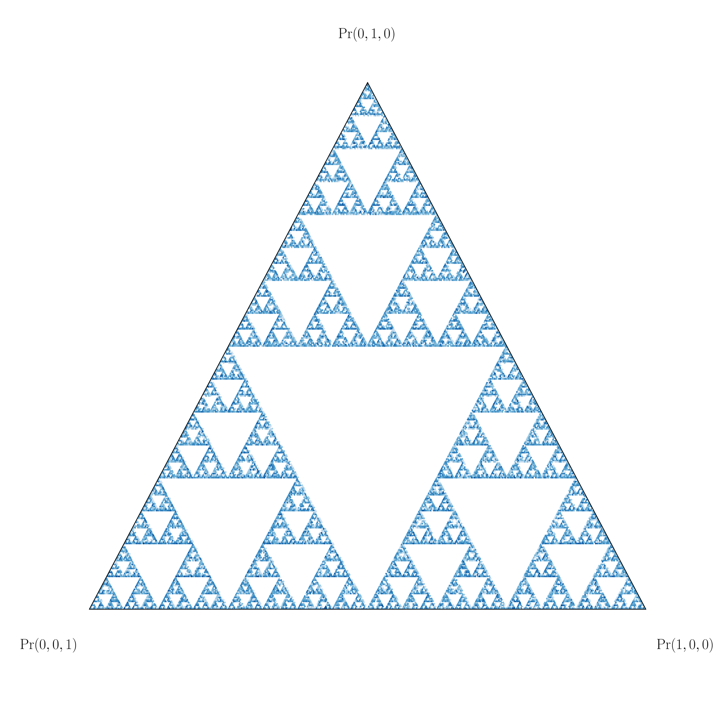
Figure S2: Attractor of the $3$-state, $3$-symbol machine specified in Eq. S6, with $s=2$ and $a=\frac{1}{6}$.

Setting $s=2$ and $a=1/6$, results in equal probability for all maps and gives the standard Sierpinski triangle shown in Fig. S2. In this case, the entropy rate is $h_{\mu}=\log_{2}3$ and the Lyapunov exponents are both $-\log_{2}2$. Plugging this into Eq. 13 returns the well-known fractal dimension of the Sierpinski triangle: $\log_{2}3/\log_{2}2\approx 1.585$.

Appendix E Lyapunov Exponents

A Lyapunov characteristic exponent for a dynamical system measures the exponential rate of separation of trajectories that begin infinitesimally close. Since, typically, the separation rate depends on the direction of the initial separation, we use a spectrum of Lyapunov exponents, with one exponent for each state-space dimension. In a chaotic dynamical system, at least one Lyapunov exponent is positive. In general, the Lyapunov exponent spectrum for an $N$-dimensional dynamical system with mapping $x_{n+1}=F(x_{n})$ depends on the initial condition $x_{0}$. However, here we consider ergodic systems, for which the spectrum does not.

Consider the map’s Jacobian matrix:

$$J=\frac{\partial F}{\partial x}$$

and the evolution of vectors in the tangent space, controlled by:

$$\dot{Y}=YJ~{},$$

where $Y(0)=\mathbb{I}_{N}$ and $Y(t)$ describes how an infinitesimal change in $x(0)$ has propagated to $x(t)$. Let $\{y_{1},\dots,y_{N}\}$ be the eigenvalues of the matrix $Y(t)Y(t)^{\intercal}$. Then, the Lyapunov exponents are:

$$\lambda_{i}=\lim_{t\to\infty}\frac{1}{2t}\log y_{i}~{}.$$

The Lyapunov numbers were introduced and proven to exist by Oseledets [60]. The Lyapunov exponents are merely the logarithms of Lyapunov numbers.

The most common way of calculating an IFS’s Lyapunov spectrum, employed to produce the results in Fig. 6, is the pull-back method. The basic idea is that for an IFS in the $N-1$ simplex, defined by an $N$-state HMC, there will be $N-1$ independent directions of contraction. These directions are represented by a coordinate frame of $N-1$ vectors that are kept orthogonal and normalized. This coordinate frame is carried along a long orbit of the IFS. At each time step, the Jacobian is used to evolve the frame. We track the contraction rate of each vector, and this becomes the estimation of the Lyapunov exponents.

In contrast to applying this approach to deterministic dynamical systems, as is more familiar, an IFS’s stochastic nature introduces additional error. Since the Jacobian varies not just across the simplex, but also for the selected maps, the orbit must be long enough to sample from the IFS attractor’s distribution accurately for each possible mapping function. This being said, it has been established that the pull-back method works for IFS spectra, given a sufficiently long orbit [61].

The prequel, on estimating the entropy rate of HMC processes, made use of error-bounding techniques from Markov chain Monte Carlo (MCMC) [32]. Since here we are estimating Lyapunov exponents by sampling from the Blackwell distribution, similar error-bounding techniques apply. In this analysis, there are two fundamental sources of estimation error. First, that due to initialization bias or undesired statistical trends introduced by the initial transient data produced by the Markov chain before it reaches the desired stationary distribution. Second, there are errors induced by autocorrelation in equilibrium. That is, the samples produced by the Markov chain are correlated. And, the consequence is that statistical error cannot be estimated by $1/\sqrt{N}$, as done for $N$ independent samples.

Bounding these error sources requires estimating the autocorrelation function, which can be done from long sequences of samples. If we have the nonunifilar model in hand, it is a simple matter of sweeping through increasingly long sequences of generated samples until we observe convergence of the autocorrelation function. An alternative method of approximating the infinite-state HMC with a finite-state approximation is discussed in detail in our previous work [32]. The upshot is that the method here generally efficiently leads to accurate estimates of the LCE spectrum.

For completeness, we note that there are alternative methods to calculate Lyapunov exponents; see, e.g., Refs. [62, 63]. These methods may be more appropriate in specific applications. That said, the accuracy and applicability of Lyapunov exponent estimation is not the focus here.

Appendix F Overlap Estimation

To estimate the size of a mixed-state attractor and overlap of mapping functions in Fig. 6, a combination of techniques were used. We will briefly summarize the method here.

First, $250,000$ different HMCs were generated using a $500\times 500$ parameter grid over $\alpha=[0,1]$ and $x=[0,0.5]$. Each HMC was defined by plugging the appropriate parameter values into the symbol-labeled transition matrices in Section VI. From this HMC, the mapping and probability functions were defined (see Eqs. 7 and 6), producing a place-dependent IFS.

For each IFS and associated HMC, $10,000$ mixed states were generated from an initial randomized state, throwing away the first $5,000$ as transients. Using a spatial algorithm from the SciPy Python package, a convex hull was drawn around this set of points, with a small buffer. This convex hull (the attractor “outline”) was converted into a polygon. This polygon was then evolved independently by each symbol-labeled mapping function, producing three polygons, each associated with a symbol. This may be visualized by referencing Fig. 5, where the evolved polygons are depicted on top of the mixed-state attractor, each with a different color. We can see that the combination of these polygons must necessarily cover the attractor.

These three symbol-labeled polygons were then combined into a single polygon or multipolygon (a polygon with “holes” that are themselves polygons) using the geometry-processing module Shapely [64]. This produces a more accurate outline of the attractor than the convex hull. This process may then be repeated with the new outline for as many iterations as desired, until a polygon or multipolygon that covers the mixed state attractor with the desired level of accuracy is produced. The same result could be achieved by beginning with the entire simplex as the initial outline, without any production of mixed-states. However, the step of estimating the convex hull sharply reduces the number of required iterations and, more importantly, makes the required number more equal across parameter space. To see this, consider that attractors taking up less of the simplex require several iterations to converge to the small size of the attractor. By initializing with the convex hull, the process of converging to the attractor’s basic shape is skipped, and the iterations are merely refinements.

In producing Fig. 6, we found that we could determine good outlines across parameter space by evolving the convex hull three times. To produce Fig. 6a, the area of the resultant polygon or multipolygon was found using Shapely. To produce Fig. 6d and Fig. 6d, the outline was evolved one more time by each map, and the resultant polygons and/or multipolygons were checked for intersection. For the binary overlap/no-overlap plot in Fig. 6d, only the existence of overlap somewhere on the attractor was considered. For the percentage overlap in Fig. 6c, the area of the total outline that was comprised of overlapping polygons—whether only two or all three—was compared to the total area. The subtlety of whether an overlap region included two or three maps was largely ignored here, but will be analyzed in future explorations of the overlap problem.