Simulating complex networks in phase space: Gaussian boson sampling
Abstract
We show how phase-space simulations of quantum states in a linear photonic network permit the verification of measurable probabilities and entanglement. We compare our predictions with recent Gaussian boson sampling experiments of Zhong et al. These use squeezed inputs and efficient “on-off” detectors, with up to -th order measured coincidence counts in the data. We introduce a general definition of grouped “on-off” detection probabilities for this purpose. The positive- phase-space method is used to compute any grouped or marginal click probabilities. Additional decoherence is included to obtain agreement between theory and experiment. The only limitation in estimating grouped probabilities is the computational sampling error, which is similar in magnitude to the experimental sampling error. The results obtained and graphed here are from first-order up to 16 000-th order grouped count probabilities. However, any order between these is also computable. We extend these results to include grouped probabilities with multidimensional outcomes that have a polynomial number of points. We also analyze quadrature detection experiments, and show how to simulate genuine multipartite entanglement using Wigner phase-space methods.
I Introduction
Bosonic quantum networks are increasingly useful in quantum technology and quantum computing applications [1]. Linear networks driven either by nonclassical number state [2, 3, 4, 5, 6, 7, 8] or Gaussian inputs [9, 10, 11, 12] for boson sampling are becoming widely available. The squeezed-state interferometer, which is a two-mode linear network, is being employed to enhance gravitational-wave detection sensitivity [13, 14]. More complex photonic networks are under development, both as novel interferometers [15, 16] and as test-beds for multipartite entanglement [17, 18, 19]. Other examples include the Ising machine, used to solve large NP-hard optimization problems [20, 21, 22].
A dramatic increase in scale of a boson sampling quantum network has recently been achieved. Zhong et al. [23] implemented a -mode Gaussian boson sampler (GBS) with squeezed inputs, and detected the output photon counts, whose distribution is called the ’Torontonian’. They measured up to -th order coincidence counts in the outputs, which they estimated to take billion years to simulate conventionally on the world’s fastest current supercomputer. This has led to reports of quantum supremacy by Zhong et al.: that is, a quantum device implementing a computational task that is not classically feasible [24, 25]. Similar reports have been made using quantum logic gates [26].
There is an ongoing debate on how to rigorously validate such technology [27, 28]. Validation based on low-order correlations [29] or direct classical simulation may be susceptible to mock-ups. However, Gaussian inputs to linear networks [9, 30] have a non-computable discrete count probability for large mode number. The output distribution is a Hafnian [10] for photon-number-resolving detectors. In the “on-off” or saturable detector case, it is the Torontonian [11]. Quesada et al. [11, 31] explained that classical evaluation of the ideal “Torontonian” distribution is exponentially complex, making it nearly impossible for more than modes [32].
Since a direct simulation of the output correlations at large cannot be achieved in less than exponential time, another approach is needed to compare theory with experiment in a reasonable timeframe. Theoretical benchmarks are essential, both to know what output is expected, and to understand any other physics.
The objective of this paper is to do simply this: to investigate whether the theory agrees with experiment. We show how one may in part solve this problem, by simulating Gaussian boson linear networks in quantum phase space. This provides a way to verify the output quantum correlations and marginal probabilities, both in the idealized case and with other known physics included. It is important to note that we do not simulate the experiment directly using discrete photon counts [11, 31]. Rather, we verify observable, grouped probabilities by averaging over many random trajectories in phase space [33], which have the same correlations and marginal probabilities.
By contrast, an explicit simulation with discrete counts is feasible, but is currently limited to either small networks or large decoherence [34]. Our methods provide a way to certify the measurable probabilities of experimental outputs, even for systems much larger than the current experimental ones. The phase space approach uses the correctness of quantum mechanics under a change of basis state to develop an alternative, powerful algorithm for efficient verification of any grouped count distribution. We have computed all of the grouped probabilities measured by Zhong et al. [23], including -th order coincidence counts, as well as other marginal probabilities in their data. We calculate these from the model of the apparatus and experimental parameters measured by the experimentalists.
Differences between theory and experiment appear to be caused by input pulse decoherence effects. Our phase-space simulations agree much better with experimental count distributions [23] after including these decoherence effects, and are scalable. Chi-squared tests were carried out [35, 36], which show an improvement of three orders of magnitude for theoretical agreement with experiment.
Results are also obtained for up to mode devices. Computational times and sampling errors are comparable to those in experiments for the same number of samples, making them useful for validation of GBS experiments. We computed marginal, low-order probabilities, as well as higher order, measurable grouped probabilities. Our methods can also be extended if necessary to include other known physics, including multiple frequency modes, dispersion, nonlinearity, decoherence and Raman/Brillouin scattering [37], allowing better understanding of these experiments.
Boson sampling outputs are exponentially hard to generate numerically. Here, we demonstrate how measurable grouped probabilities can be verified. A key feature of quantum mechanics which allows this in GBS is that binary “click” measurement operators are multimode projection operators, whose averages are probabilities. The positive- phase-space representation allows one to calculate these probabilities using efficient phase-space sampling methods, even though a direct sampling of the click distribution is exponentially hard. Since methods used to detect eavesdroppers involve measurement of moments or probabilities, this also suggests relevance to cryptographic steganography, in which messages could be hidden in the random outputs. We further demonstrate, using simulations in a different phase-space, the Wigner representation, how to certify the genuine -partite entanglement of all nodes of a Gaussian network.
II Gaussian bosonic networks
We consider an mode bosonic network, with squeezed-state inputs to out of modes. A linear, unitary transformation is made to a set of output modes, combined with decoherence and losses. Measurements are carried out on the output state . The theoretical problem is to calculate quadrature correlations and binned counts for the output quantum state. To solve this, we utilize discrete Fourier transform methods for ensemble averages of grouped photon counts [33].
A squeezed-state is a minimum uncertainty state in which one of the input mode quadratures has its fluctuations reduced below the vacuum noise level [38, 39, 40]. We suppose that the squeezing of for each excited mode is in the imaginary part of . If each input is independent, the quantum state can be factorized into a product of single-mode states. Defining input quadrature operators , , so that , the quantum inputs are defined by a squeezing vector
The variances in each mode are:
| (1) |
The input photon numbers are , with coherences of . Pulsed squeezing [41] involves multiple longitudinal modes, with mismatches in time or frequency [23], as well as phase noise [42]. We model this experimental decoherence by an intensity transmissivity into the network, combined with a thermal input of uncorrelated photons per mode. Our model is similar to thermal squeezing [43], except with an invariant photon number.
The overall result is that the photon number is unchanged, and the coherence of each mode is reduced so that
II.1 Phase-space representations
At large , number state expansions of the input state require exponentially many expansion coefficients to treat this. Instead, we use phase-space expansions [44] which allow a probabilistic representation of the input states. Two common phase-space approaches are used: the Wigner representation [45], and the generalized -representation [46]. These methods do not assume Gaussianity, and applications to non-Gaussian photonic networks were already demonstrated [33, 47].
II.1.1 Positive -representation
-representations are normally ordered and therefore do not have any vacuum noise, making them efficient for simulating photo-detection measurements. The most suitable technique for non-classical photon-counting measurements is the generalized -representation [46, 48], which has been applied to other large-scale bosonic simulations [49].
In this representation, is expanded over a subspace of the complex plane defined by
| (2) |
The operator basis is a off-diagonal coherent state projector onto multimode Glauber [50] coherent states, and is an integration measure on the -dimensional complex space of amplitudes , which in some cases reduce to simple real amplitudes.
For a squeezed input state , one obtains a positive P-distribution on a real subspace with , . If the input is , a product of single-mode squeezed state density matrices, the solution for a squeezed state, based on one-dimensional coherent state expansions [51] is:
| (3) |
where the normalization constant is
In this approach, normally ordered operator moments are equivalent to stochastic moments [46], so that with quantum expectation values denoted , and probabilistic averages with samples denoted .
To create input samples for a squeezed state distribution , one uses real Gaussian noises with to generate random phase-space samples . The stochastic model for a pure or thermalized squeezed state, , is given by [42]:
| (4) |
The coefficients must satisfy , which gives real amplitudes for , and complex amplitudes for .
II.1.2 Wigner representation
Other possible phase-space methods include the Wigner [45, 52] and Q-function [53], methods with symmetric and anti-normal ordering respectively. These give exponentially larger sampling errors [42] for intensity correlation due to their extra vacuum noise, while the Glauber P-representation is singular for squeezed states. These methods have a classical phase-space, in which . The Wigner representation is best for analyzing multipartite entanglement, with data coming from quadrature measurements [54, 55, 56], which have been carried out at an increasingly large scale [57, 17, 18, 58, 19].
For an input quantum density matrix the Wigner distribution is written most compactly as [59, 44, 60]:
| (5) |
More generally, -ordered classical bosonic representations [61] are defined using an parameter signifying the relative amount of vacuum noise, with for normal ordering or P-representations and for symmetric ordering or Wigner representations. For pure and thermalized squeezed state inputs [62, 42], the -ordered classical phase-space stochastic amplitude is
| (6) |
where has the requirement that:
| (7) |
II.2 Network Transmission
Once a set of input states is simulated, it can be transformed and used to sample the output state in any of these representations. An input density matrix is changed by a linear photonic network to an output density matrix . For unitary transformations , the phase-space amplitudes are transformed deterministically, where , in all representations. In the generalized P-representation one may include a non-unitary transmission matrix to take account of losses, which is equivalent to a master equation [63].
For normal ordering in a linear network, the output density matrix has a simple form [64], including linear couplings and losses:
| (8) |
The input distribution may no longer be restricted to the real axes if there are input thermal photons included to model decoherence with .
For other types of ordering, vacuum noise must be included from the reservoirs that couple to the system modes, causing decoherence. This is achieved by noting that for a vacuum state, the input and output correlations are identical, and for -ordering, It is therefore necessary to add additional vacuum noise if and is non-unitary. This is achieved through defining an hermitian decoherence matrix, , which has a decomposition , where is diagonal and positive. The matrix square root is and the output amplitudes are:
| (9) |
This ensure that vacuum noise is unchanged.
III Quantum measurements
We consider two type of measurements in detail, namely quadrature detection, and efficient photo-detectors that saturate for more than one count.
III.1 Phase-space representations of measurement operators
III.1.1 Quadrature detectors
For quadrature detection, the quadrature phase amplitudes of each output mode are , with special cases, for of and , in a rotating frame. The measurable quadrature correlations are , where , and :
| (10) |
This is directly simulated in the Wigner representation. The phase-space variables are and the correlations are calculated by replacing , and averaging over the Wigner function.
III.1.2 Photon number detectors
For photon number resolving photodetectors, the output number operator is . The -th order Glauber correlation function is [50] :
| (11) |
where is the number of counts at the -th detector, and is the total measurement order. The corresponding phase-space observable is obtained by replacing , where is the output number variable, sampled with probability . To calculate the output number distribution, there are a number of methods [10], for transforming these correlations into the observed distributions, but in this paper we focus on the saturating, or on-off detector, as recent experiments use this type of measurement.
For saturating photodetectors, all non-zero counts give an identical output. The “on-off” click projection operator is [65] :
| (12) |
where is the number of measured counts at the -th detector, and the output number operator is . Multi-mode results are given by an -digit binary number . This has possible patterns available. For a set of sites, each binary number has an -order correlation operator of The corresponding expectation,
| (13) |
is the Torontonian function [11] for Gaussian inputs, if the set of sites corresponds to all output channels. As this is normally ordered, it has a direct correspondence with a phase-space function in the positive P-representation. The phase-space observable is given by replacing , where is the output number variable sampled with probability .
In all cases, the corresponding -th order moment is simulated by replacing with the randomly sampled complex number . We note that the operators are projectors. As a result, their expectations are the probabilities [66] of measuring the count pattern
Since there are exponentially many possible count patterns , the probability of measuring any individual pattern, , becomes infinitesimal for large . A direct measurement cannot obtain all such correlations in less than exponential time. Thus, it is hard to calculate all probabilities, and it is also hard to measure them [33, 47].
III.1.3 Grouped or marginal probabilities
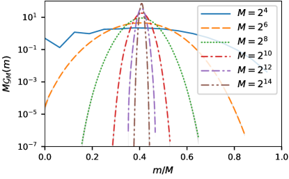
Grouped counts are therefore essential for verifying GBS statistics at large , in order to obtain measurable probabilities. One must simulate and measure the -th order grouped probabilities, , where , is the total probability order [50], and:
| (14) |
These are the -dimensional grouped count probabilities of observing grouped counts in disjoint sets of output modes. If , they include low-order marginal probabilities often proposed for verification purposes, with outputs ignored. The first-order correlation with , is the count probability in the -th channel. Similarly, and gives the Torontonian. For sequential channel groups, the sets are simply denoted by their sizes . Using this notation, is the probability for observing clicks in any pattern, as reported in recent experiments [23].
We use the terminology of quantum optics [50] to define the measurement order, , since the binned correlations involve simultaneous measurements at different sites. However, the are probabilities obtained from some or all of the detectors. One can extract moments from the resulting distributions, and the resulting statistical moments can also have various orders from . It is important to distinguish the original measurement order which depends on the number of modes, from the statistical moment orders that are extracted later.
Calculating these quantities appears intractable at first: how can one compute the sum of exponentially many terms, if each is exponentially hard? Yet, high-order correlations are readily simulated on replacing the operator by the phase-space variable , and averaging over the probability . The summation over grouped correlations is achieved through defining angles , with a Fourier observable defined for , where . The grouped probability is then obtained from a -dimensional inverse discrete Fourier transform, so that:
| (15) |
All combinations of terms vanish in the inverse Fourier transform except those terms with counts. This algorithmic procedure is highly scalable. To demonstrate this, two simulation codes were written and tested. Exact Torontonians were simulated for small networks. Analytically tractable inputs were used to test large networks. Excellent agreement was found in all cases.
To demonstrate this technique for quantum squeezed inputs, we graph the grouped count probability in Fig (1) for sizes up to , using squeezed states with , , for inputs, and random unitaries.
IV Grouped count verification in GBS experiments
The grouped probabilities provide a signature of a quantum state. Clearly, they must be measurable and have a low sampling error. To validate results, the theoretical sampling error must be less than the experimental sampling error , where the experimental sampling error depends on the number of samples used, and scales as . Experiment and simulations have similar time-scales for comparable error-bars.
Due to internal averaging, single group measures are less sensitive to the unitary as increases, but are very sensitive to decoherence. Count “fingerprints” with more groups are also needed for a complete test, and one is computed below. Many such measures are available, both from experimental data and from simulations.
IV.1 Comparisons with a GBS experiment
To compare theory to experiment, squeezing vectors and transmission data from a recent mode Gaussian boson sampling experiment were obtained [23] and simulated with samples. The data was a mode vector of amplitudes , a transmission matrix , and measured click patterns. The experimental data was used to calculate grouped correlations, and compared to simulations with a standard chi-squared test [67], using a lower cut-off of 10 counts per bin [68, 36]. Statistical methods and tests of the codes are given in the Appendix.
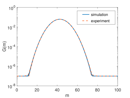
For significant bins, one expects . Simulating total counts, , with pure squeezed-state inputs gave a large chi-squared value of , with valid data points. Additionally, we tested a mode fully thermalized model. This gave an even larger discrepancy. The chi-squared value was , confirming a prediction [69] that one can distinguish boson sampling from uniform distributions.
Better agreement with experiment was obtained with a small admixture of thermal inputs. For optimal fitting, we included an thermal component to model longitudinal mode mismatching. Transmission amplitudes were multiplied by . Results of simulations are given in Fig (2). This agrees with experiment over a range of six orders of magnitude in the measurable grouped probabilities. A chi-squared value of was obtained, giving three orders of magnitude lower values than with pure state inputs. Residual discrepancies may be from nonlinearities.
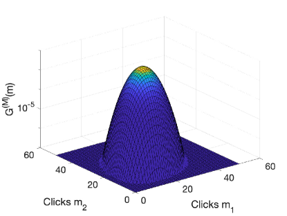
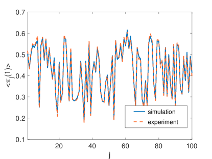
Fig (3) shows , which is a two-dimensional binning of the -th order probabilities. Any number of bins - up to - are feasible in principle. However, experimental sampling errors increase as the grouping dimension increases, giving a limit of dimensions with currently available experimental data. As another comparison, the marginal count probability per channel , is graphed in Fig (4). This also shows good agreement with experiment.
IV.2 Detailed statistical comparisons
We now consider the details of the comparisons and the inferred decoherence from the grouped -th order correlations in a GBS experiment, as compared to a phase-space simulation. We wish to compare two hypotheses. The first, , is that the correlations are given by the experimental squeezing and transmission matrices. The second, , is that there is additional decoherence, modeled by an thermal fraction , with an unchanged photon number.
In both cases, the experimental counts are the same. However, graphing raw experimental and theoretical count probabilities is not useful for comparative purposes, as the probabilities appear nearly identical to the naked eye [67]. Due to the accuracy of the data, with over total counts, it is much more useful to graph the normalized deviation between theoretical and experimental probabilities, as described in the Appendix:
| (16) |
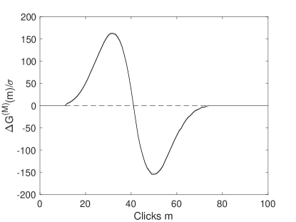
For good agreement between theory and experiment, one expects a normalized difference of unity. Figure (5), shows the normalized discrepancy between theory and experiment in , in a simulation having no decoherence. An inspection of the graph shows very significant differences between the theoretical and experimental count probabilities, with . This is reflected in the results for the null hypothesis , where one obtains an extremely large value of , out of valid data points having more than counts. This gives a discrepancy ratio of .
Clearly, when decoherence is excluded, the experiment strongly disagrees with a simple, coherent GBS model. Therefore, the hypothesis of no decoherence, apart from losses, has a vanishingly small probability. The hypothesis of a fully thermal model with is less likely still. With this model, the total discrepancy ratio is . Hence, the output is easily distinguishable from a thermal one [69].
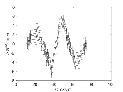
Figure (6), shows the differences in , between experimental and simulated probabilities with a small decoherence of , as described above. The transmission amplitude was increased by a factor of to improve the fit. This is a small correction, since even small deviations can result in large chi-squares. The new graph shows much smaller differences between the theoretical and experimental count probabilities, with .
For the hypothesis , with additional decoherence, the value is . The total ratio is , more than times smaller than for a pure state. This indicates that the hypothesis of additional decoherence is more compatible with experimental measurements. These results show good agreement with a model of GBS including a small thermal decoherence. Other physical effects including nonlinearities may explain the remaining discrepancies.
The phase-space errors here were less than the experimental errors, and could be reduced further, at the cost of longer computation time. There were times more experimental than theoretical samples. Hence, this simulation is comparable or better than experimental efficiency. The error ratio depends on the observations.
The same technique is applicable to any measurable distribution, including lower order marginal probabilities and multiple partitions. We plotted an example of a two-dimensional grouped probability distribution in the previous subsection. This has similar properties, with a distribution close to the experimental one, and includes thousands of data points.
In general it is possible to check the GBS hypothesis for any set of parameters and marginal or grouped probability distributions. Measurable, grouped probability distributions of GBS experimental data can be simulated to high accuracy. We have simulated correlation orders from first up to 16,000th order. The computational time depends on the complexity of extraction of the binned correlations, and on the error requirements.
There are many correlation tests possible. Thus, to disprove a classical mock-up, one could simply use a large, randomly chosen subset of tests of all orders. Just as with other RNG tests, it is increasingly unlikely that a range of statistical tests like this can be faked. We conjecture that the multidimensional grouped probabilities, as in Fig 3, have the most potential for this due to their polynomially large number of probability samples.
V N-partite entanglement
These experiments typically lead to entangled outputs. However, the entanglement is demonstrated most directly using a different type of measurement. We will illustrate this for one type of -partite entangled state that is generated from one or two squeezed vacuum states. In this section, we briefly outline the known method for generating such a state [54, 56]. In short, the squeezed inputs are first combined across a single beam splitter to create a two-mode Einstein-Podolsky-Rosen (EPR) entangled state [70]. One of the outputs is then passed through beam splitters [54, 56].
V.1 Multi-mode entanglement theory
The overall set-up has inputs , where the first two inputs are orthogonally squeezed vacuum states. In particular, is a squeezed vacuum input with , and is squeezed vacuum input with . Here is the squeezing parameter. All other inputs are vacuum states, implying . The inputs are combined across a total of beam splitters. We use the notation to mean the variance of i.e. .
To create two-mode EPR entanglement, inputs and are passed through beam splitter , with reflectivity and , according to
| (17) |
The output of is . It is straightforward to show using the approach developed in [70] that the two outputs are EPR correlated with respect to the quadrature phase amplitudes, i.e.
| (18) |
More details are given in [71, 72], where EPR steering is also considered. For large , both variances become zero. EPR entanglement can also be created from one squeezed input to give
| (19) |
To generate multipartite entanglement, the field is combined across a second with reflectivity and , according to [54]
| (20) |
The output of field is . For , there are only two beam splitters, and the output of is . For , the process continues with another beam splitter
| (21) |
The output of mode is and the output of mode is .
It is possible to continue in this way, and to select the reflectivities of a string of beam splitters so that we obtain, from two squeezed inputs, the following solution for the final outputs , given by , and :
| (22) |
To achieve this, the reflectivity for -th beam splitter, where , is , , for , with . This is explained in more detail in [54, 56].
V.2 Unitary matrix
The corresponding unitary matrix for the set-up is obtained by first introducing a vector of reflection amplitudes, defined by
| (23) |
We express the transformation of the input modes into genuinely entangled output modes as a unitary matrix . The output modes are
| (24) |
Defining and , the elements of the unitary matrix for are given by:
| (25) |
V.3 N-partite entanglement simulations
We now consider how to use phase-space simulations to model an entangled bosonic network, such as the one described in the last section. This result can be readily simulated, and we find that one can verify genuine -partite entanglement [54, 56], where we take . The optimal simulation method is the Wigner representation, which for quadrature measurement is the natural approach, requiring no ordering corrections. Other methods gave larger sampling errors. As one might guess intuitively, it is optimal to use the representation that matches the measurement operator [73].
This case demonstrates the high efficiency of Wigner phase-space methods for simulating quadrature measurements, although it is a completely different type of measurement to the click detection often used in GBS.
We follow the definitions given in Eq. (22). Let and , then the observation of
| (26) |
confirms -partite entanglement for all . The observation of
| (27) |
also confirms -partite entanglement for all . The proof of the latter inequality is given in [54], for full tripartite inseparability. The proofs for genuine -partite entanglement, and for the first inequality involving a product, follow along similar lines, using the methods developed in [56]. The detailed proofs of these threshold points will be given elsewhere [71].
The above inequalities suffice to confirm the -partite entanglement of the fields created by the ideal network, but other methods of detection are also possible [55, 74, 75]. This is particularly true if one assumes pure or Gaussian states, or is interested to measure full -partite inseparability only [55, 74, 76, 17, 57, 75].
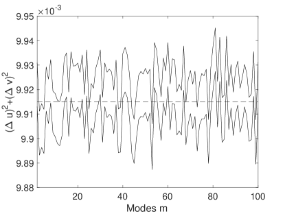
Figure (7), shows the result of a Wigner simulation of multipartite entanglement, plotted against the number of input modes, for and samples. The total ratio of , for 99 data points, showing that the simulation is consistent with the analytic result. The simulation error bars are . The threshold for the signature in this case is at , so the criterion is satisfied.
This level of precision are not obtained for all phase-space methods. In a positive-P simulation of multipartite entanglement, otherwise identical to figure (7) the total chi-squared ratio was , for independent points, indicating agreement with the analytic result, but the sampling error bars were , which is times larger. Similar large errors are found for the Q-function. In both cases, one must add or subtract corrections to transform the variance to symmetric ordering, which leads to larger sampling errors.
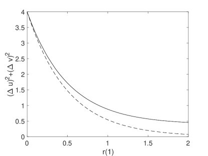
Phase-space simulations can readily include losses, decoherence and inhomogeneity. These all impact the amount of input squeezing required in realistic experiments. A simple example is shown in Fig (8) which simulates an input coupling amplitude transmission of . This is sufficient to prevent the multipartite signature from being achieved for an network, with .
VI Summary
In summary, we have simulated Gaussian bosonic networks with phase-space methods. This efficiently simulates large networks with nonclassical inputs and decoherence. Up to modes were treated. There is excellent agreement with a recent -mode Gaussian boson sampling experiment for the total count probability, provided thermal decoherence is included. Other tests, including arbitrary order marginals, are also possible. The main limitation is that the phase-space sampling errors can be significant if the grouped probabilities are too small, but it is straightforward to increase sample numbers to reduce this. Similar limitations due to sampling error hold for the experimental data as well,
More generally, the representation used should be targeted to the measurement. Positive P-representations are optimal for normally ordered photo-detectors used in Gaussian boson sampling, while Wigner representations scale better for quadrature measurements and entanglement. Following the submission of our work, preprints have appeared covering related topics [77, 78], including calculations of low order marginals of grouped distributions, and improved direct sampling methods.
Acknowledgements.
PDD thanks Jian-Wei Pan for access to experimental data. Corrected results were downloaded on Oct 4, 2021. Large-scale calculations were performed on the OzSTAR national supercomputing facility funded by Swinburne University of Technology and the Australian National Collaborative Research Infrastructure Strategy (NCRIS). This work was also funded through an Australian Research Council Discovery Project Grant DP190101480, and a grant from NTT Research.Appendix: Statistics and numerical validation
Statistical tests
Statistical tests are essential in comparing theory to experimental data. In this paper, we compare phase-space simulations both with exactly known distributions, and with mode experimental observations. The test procedures are similar in both cases. We use chi-square methods originally discovered by Pearson [67], which are widely used in probability and RNG validation [68, 36]. Other tests of probability difference are also feasible, since our techniques generate complete number distributions, but chi-square tests are preferable for sampled data because they take account of experimental sampling errors.
Chi-square tests are used to compare a theoretical probability distribution to a set of experimental measurements [67], and can also be used to compare two independent samples. In these tests, experimental observations are grouped into disjoint classes, with frequencies (for ), from observations.
Let an hypothesis give a probability for an observation in the -th class. Defining an experimental probability estimate as , This has a distribution with , provided the counts all have a nearly Gaussian distribution.
Here, is the expected variance in the experimental counts, which have Poissonian fluctuations. To deal with small counts, it is commonly recommended that these should not be included if . Knuth [36] suggests , and is recommended by NIST [79, 68]. We take the middle ground, ignoring counts less that . Changing this threshold has little effect.
The true theoretical probability is not always available. In this work, we use an estimated value from phase-space simulations, which converges to in the limit of a large ensemble. The theoretical probability is estimated numerically from its ensemble mean, .
To obtain an error estimate for , it is computed numerically [33] by using sub-ensembles, each with many samples. From the central limit theorem, sub-ensemble means are nearly Gaussian distributed, with a standard deviation of . These are obtained from the simulations. As a result, the simulated ensemble mean has a standard deviation in the mean of .
This uncertainty in the true probability implies that the chi-squared test must be modified, which is similar the well-known case of two samples drawn from the same population [35, 80]. For a finite ensemble, we employ an error measure of:
| (28) |
This uses the fact that the experimental and simulated data are independent and nearly Gaussian. The difference in their means has a variance of , which is obtained by adding the two variances. Correlated fluctuations modify the effective degrees of freedom, so we do not calculate the detailed distribution. However, since , we check if .
Fluctuations in the simulated data vanish in the limit of a large simulation, because as . Such tests can be applied to any experimental probability, provided the measured data is binned to give enough counts to be significant. This requirement also includes marginal distributions which are included in our general definition.
Binned tests are also used in other RNG tests [68], which have very similar requirements. The difference between our tests and other RNG tests is that the comparisons are obtained through sampling. This is necessary because the exact Torontonian is non-computable. However, it does raise the question of how many samples are needed. This is answered by increasing the sample number until . We found that was sufficient, using 1200 sub-ensembles of 1000 samples.
Numerical validation tests
To test our numerical results, independent numerical codes for simulations were written for two different languages (Matlab and Python) and computational platforms (a 14 core desktop, and a supercomputer with GPU hardware). Simulations were checked against known Torontonians for 16-mode networks with squeezed inputs [11, 81]. The mode, million sample phase-space simulations took on a current desktop computer.
We validated the theoretical code in larger cases by comparison to exact analytic results for squeezed, thermalized and thermal inputs. Both unitary and lossy transmission matrices were used, and homogeneous or inhomogeneous squeezed inputs. For and matrices, different types of moment were tested with up to four-dimensional binning.
A typical example output is plotted in Fig (9), which shows a test for a thermalized input with and , using a random unitary transmission matrix. The output is the probability for a order correlation, binned four ways, to give click patterns. The graph is a two-dimensional slice in the plane, with and , of the normalized error.
Plotted data was all within . The overall test gave in significant data points (, out of possible click patterns. These results show complete agreement with the analytic probability model.
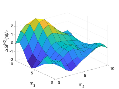
For each matrix, 68 distinct tests with up to data points were carried out, in P, Q and Wigner phase-space. Probability cutoffs were used of , with total samples, since small probabilities are non-Gaussian. This effect is reduced by increasing the ensemble size. The overall result for matrices was . This agrees with analytic tests, with evidence for nearly Gaussian errors.
References
- Scheel [2005] S. Scheel, in Quantum Information Processing, edited by T. Beth and G. Leuchs (Wiley-VCH, Weinheim, 2005) Chap. 28, pp. 382–392.
- Aaronson [2011] S. Aaronson, Proceedings of the Royal Society of London A: Mathematical, Physical and Engineering Sciences 467, 3393 (2011).
- Broome et al. [2013] M. A. Broome, A. Fedrizzi, S. Rahimi-Keshari, J. Dove, S. Aaronson, T. C. Ralph, and A. G. White, Science 339, 794 (2013).
- Crespi et al. [2013] A. Crespi, R. Osellame, R. Ramponi, D. J. Brod, E. F. Galvao, N. Spagnolo, C. Vitelli, E. Maiorino, P. Mataloni, and F. Sciarrino, Nature photonics 7, 545 (2013).
- Tillmann et al. [2013] M. Tillmann, B. Dakić, R. Heilmann, S. Nolte, A. Szameit, and P. Walther, Nature photonics 7, 540 (2013).
- Spring et al. [2013] J. B. Spring, B. J. Metcalf, P. C. Humphreys, W. S. Kolthammer, X.-M. Jin, M. Barbieri, A. Datta, N. Thomas-Peter, N. K. Langford, D. Kundys, et al., Science 339, 798 (2013).
- Spagnolo et al. [2014] N. Spagnolo, C. Vitelli, M. Bentivegna, D. J. Brod, A. Crespi, F. Flamini, S. Giacomini, G. Milani, R. Ramponi, P. Mataloni, et al., Nature Photonics 8, 615 (2014).
- Crespi et al. [2016] A. Crespi et al., Nat. Commun. 7, 10469 (2016).
- Lund et al. [2014] A. P. Lund, A. Laing, S. Rahimi-Keshari, T. Rudolph, J. L. O’Brien, and T. C. Ralph, Phys. Rev. Lett. 113, 100502 (2014).
- Hamilton et al. [2017] C. S. Hamilton, R. Kruse, L. Sansoni, S. Barkhofen, C. Silberhorn, and I. Jex, Phys. Rev. Lett. 119, 170501 (2017).
- Quesada et al. [2018] N. Quesada, J. M. Arrazola, and N. Killoran, Physical Review A 98, 062322 (2018).
- Kruse et al. [2019] R. Kruse, C. S. Hamilton, L. Sansoni, S. Barkhofen, C. Silberhorn, and I. Jex, Physical Review A 100, 032326 (2019).
- Caves [1981] C. M. Caves, Physical Review D 23, 1693 (1981).
- McCuller et al. [2020] L. McCuller, C. Whittle, D. Ganapathy, K. Komori, M. Tse, A. Fernandez-Galiana, L. Barsotti, P. Fritschel, M. MacInnis, F. Matichard, K. Mason, N. Mavalvala, R. Mittleman, H. Yu, M. E. Zucker, and M. Evans, Physical Review Letters 124, 171102 (2020).
- Motes et al. [2015] K. R. Motes, J. P. Olson, E. J. Rabeaux, J. P. Dowling, S. J. Olson, and P. P. Rohde, Phys. Rev. Lett. 114, 170802 (2015).
- Su et al. [2017] Z.-E. Su, Y. Li, P. P. Rohde, H.-L. Huang, X.-L. Wang, L. Li, N.-L. Liu, J. P. Dowling, C.-Y. Lu, and J.-W. Pan, Phys. Rev. Lett. 119, 080502 (2017).
- Chen et al. [2014] M. Chen, N. C. Menicucci, and O. Pfister, Phys. Rev. Lett. 112, 120505 (2014).
- Roslund et al. [2014] J. Roslund, R. M. De Araujo, S. Jiang, C. Fabre, and N. Treps, Nature Photonics 8, 109 (2014).
- Yoshikawa et al. [2016] J.-i. Yoshikawa, S. Yokoyama, T. Kaji, C. Sornphiphatphong, Y. Shiozawa, K. Makino, and A. Furusawa, APL Photonics 1, 060801 (2016).
- Marandi et al. [2014] A. Marandi, Z. Wang, K. Takata, R. L. Byer, and Y. Yamamoto, Nature Photonics 8, 937 (2014).
- Inagaki et al. [2016] T. Inagaki, Y. Haribara, K. Igarashi, T. Sonobe, S. Tamate, T. Honjo, A. Marandi, P. L. McMahon, T. Umeki, K. Enbutsu, et al., Science 354, 603 (2016).
- Yamamoto et al. [2017] Y. Yamamoto, K. Aihara, T. Leleu, K.-i. Kawarabayashi, S. Kako, M. Fejer, K. Inoue, and H. Takesue, npj Quantum Information 3, 1 (2017).
- Zhong et al. [2020] H.-S. Zhong, H. Wang, Y.-H. Deng, M.-C. Chen, L.-C. Peng, Y.-H. Luo, J. Qin, D. Wu, X. Ding, Y. Hu, et al., Science 370, 1460 (2020).
- Bremner et al. [2016] M. J. Bremner, A. Montanaro, and D. J. Shepherd, Phys. Rev. Lett. 117, 080501 (2016).
- Boixo et al. [2018] S. Boixo, S. V. Isakov, V. N. Smelyanskiy, R. Babbush, N. Ding, Z. Jiang, M. J. Bremner, J. M. Martinis, and H. Neven, Nature Physics 14, 595 (2018).
- Arute et al. [2019] F. Arute, K. Arya, R. Babbush, D. Bacon, J. C. Bardin, R. Barends, R. Biswas, S. Boixo, F. G. Brandao, D. A. Buell, et al., Nature 574, 505 (2019).
- Shepherd and Bremner [2009] D. Shepherd and M. J. Bremner, Proceedings of The Royal Society A: Mathematical, Physical and Engineering Sciences 465, 1413 (2009).
- Hangleiter et al. [2019] D. Hangleiter, M. Kliesch, J. Eisert, and C. Gogolin, Phys. Rev. Lett. 122, 210502 (2019).
- Phillips et al. [2019] D. Phillips, M. Walschaers, J. Renema, I. Walmsley, N. Treps, and J. Sperling, Physical Review A 99, 023836 (2019).
- Brod et al. [2019] D. J. Brod, E. F. Galvão, A. Crespi, R. Osellame, N. Spagnolo, and F. Sciarrino, Advanced Photonics 1, 034001 (2019).
- Quesada and Arrazola [2020] N. Quesada and J. M. Arrazola, Physical Review Research 2, 023005 (2020).
- Li et al. [2020] Y. Li, M. Chen, Y. Chen, H. Lu, L. Gan, C. Lu, J. Pan, H. Fu, and G. Yang, arXiv preprint arXiv:2009.01177 (2020).
- Opanchuk et al. [2018] B. Opanchuk, L. Rosales-Zárate, M. D. Reid, and P. D. Drummond, Physical Review A 97, 042304 (2018).
- Qi et al. [2020] H. Qi, D. J. Brod, N. Quesada, and R. García-Patrón, Physical review letters 124, 100502 (2020).
- Pearson [1911] K. Pearson, Biometrika 8, 250 (1911).
- Knuth [2014] D. E. Knuth, Art of computer programming, volume 2: Seminumerical algorithms (Addison-Wesley Professional, 2014).
- Corney et al. [2008] J. F. Corney, J. Heersink, R. Dong, V. Josse, P. D. Drummond, G. Leuchs, and U. L. Andersen, Physical Review A 78, 023831 (2008).
- Yuen [1976] H. P. Yuen, Physical Review A 13, 2226 (1976).
- Drummond and Ficek [2004] P. D. Drummond and Z. Ficek, eds., Quantum Squeezing (Springer-Verlag, Berlin, Heidelberg, New York, 2004).
- Vahlbruch et al. [2016] H. Vahlbruch, M. Mehmet, K. Danzmann, and R. Schnabel, Physical Review Letters 117, 110801 (2016).
- Raymer et al. [1991] M. G. Raymer, P. D. Drummond, and S. J. Carter, Optics letters 16, 1189 (1991).
- Drummond and Opanchuk [2020] P. D. Drummond and B. Opanchuk, Physical Review Research 2, 033304 (2020).
- Fearn and Collett [1988] H. Fearn and M. Collett, Journal of Modern Optics 35, 553 (1988).
- Hillery et al. [1984] M. Hillery, R. F. O’Connell, M. O. Scully, and E. P. Wigner, Phys. Rep. 106, 121 (1984).
- Wigner [1932] E. Wigner, Phys. Rev. 40, 749 (1932).
- Drummond and Gardiner [1980] P. D. Drummond and C. W. Gardiner, J. Phys. A 13, 2353 (1980).
- Opanchuk et al. [2019] B. Opanchuk, L. Rosales-Zárate, M. D. Reid, and P. D. Drummond, Optics Letters 44, 343 (2019).
- Drummond et al. [1981] P. D. Drummond, C. W. Gardiner, and D. F. Walls, Phys. Rev. A 24, 914 (1981).
- Drummond and Chaturvedi [2016] P. D. Drummond and S. Chaturvedi, Physica Scripta 91, 073007 (2016).
- Glauber [1963] R. J. Glauber, Phys. Rev. 130, 2529 (1963).
- Janszky and Vinogradov [1990] J. Janszky and A. V. Vinogradov, Physical review letters 64, 2771 (1990).
- Moyal [1949] J. E. Moyal, Mathematical Proceedings of the Cambridge Philosophical Society 45, 99 (1949).
- Husimi [1940] K. Husimi, Proc. Phys. Math. Soc. Jpn. 22, 264 (1940).
- van Loock and Furusawa [2003] P. van Loock and A. Furusawa, Physical Review A 67, 052315 (2003).
- Sperling and Vogel [2013] J. Sperling and W. Vogel, Physical review letters 111, 110503 (2013).
- Teh and Reid [2014] R. Y. Teh and M. D. Reid, Physical Review A 90, 062337 (2014).
- Coelho et al. [2009] A. Coelho, F. Barbosa, K. Cassemiro, A. Villar, M. Martinelli, and P. Nussenzveig, Science 326, 823 (2009).
- Armstrong et al. [2015] S. Armstrong, M. Wang, R. Y. Teh, Q. Gong, Q. He, J. Janousek, H.-A. Bachor, M. D. Reid, and P. K. Lam, Nature Physics 11, 167 (2015).
- Louisell [1973] W. H. Louisell, Quantum statistical properties of radiation (Wiley, New York, 1973).
- Drummond and Hillery [2014] P. D. Drummond and M. Hillery, The quantum theory of nonlinear optics (Cambridge University Press, 2014).
- Cahill and Glauber [1969] K. E. Cahill and R. J. Glauber, Physical Review 177, 1882 (1969).
- Olsen and Bradley [2009] M. Olsen and A. Bradley, Optics Communications 282, 3924 (2009).
- Gardiner [2004] C. Gardiner, Handbook of Stochastic Methods for Physics, Chemistry, and the Natural Sciences, Springer complexity (Springer, 2004).
- Drummond et al. [2016] P. D. Drummond, B. Opanchuk, L. Rosales-Zárate, M. D. Reid, and P. J. Forrester, Physical Review A 94, 042339 (2016).
- Sperling et al. [2012] J. Sperling, W. Vogel, and G. S. Agarwal, Phys. Rev. A 85, 023820 (2012).
- Caves and Drummond [1994] C. M. Caves and P. D. Drummond, Reviews of Modern Physics 66, 481 (1994).
- Pearson [1900] K. Pearson, The London, Edinburgh, and Dublin Philosophical Magazine and Journal of Science 50, 157 (1900).
- Rukhin et al. [2010] A. L. Rukhin, J. Soto, J. R. Nechvatal, M. E. Smid, E. B. Barker, S. D. Leigh, M. Levenson, M. Vangel, D. L. Banks, et al., A statistical test suite for random and pseudorandom number generators for cryptographic applications (2010).
- Aaronson and Arkhipov [2014] S. Aaronson and A. Arkhipov, Quantum Info. Comput. 14, 1383 (2014).
- Reid [1989] M. D. Reid, Phys. Rev. A 40, 913 (1989).
- Dellios et al. [2021] A. Dellios, P. D. Drummond, B. Opanchuk, R. Y. Teh, and M. D. Reid (2021).
- Teh et al. [2021] R. Y. Teh, M. Gessner, M. D. Reid, and M. Fadel, arXiv preprint arXiv:2108.06926 (2021).
- Dirac [1945] P. A. M. Dirac, Rev. Mod. Phys. 17, 195 (1945).
- Gerke et al. [2015] S. Gerke, J. Sperling, W. Vogel, Y. Cai, J. Roslund, N. Treps, and C. Fabre, Physical review letters 114, 050501 (2015).
- Shalm et al. [2013] L. K. Shalm, D. R. Hamel, Z. Yan, C. Simon, K. J. Resch, and T. Jennewein, Nature Physics 9, 19 (2013).
- Villar et al. [2005] A. S. Villar, L. S. Cruz, K. N. Cassemiro, M. Martinelli, and P. Nussenzveig, Physical Review Letters 95, 243603 (2005).
- Bulmer et al. [2021] J. F. Bulmer, B. A. Bell, R. S. Chadwick, A. E. Jones, D. Moise, A. Rigazzi, J. Thorbecke, U.-U. Haus, T. Van Vaerenbergh, R. B. Patel, et al., arXiv preprint arXiv:2108.01622 (2021).
- Villalonga et al. [2021] B. Villalonga, M. Y. Niu, L. Li, H. Neven, J. C. Platt, V. N. Smelyanskiy, and S. Boixo, arXiv preprint arXiv:2109.11525 (2021).
- Roscoe and Byars [1971] J. T. Roscoe and J. A. Byars, Journal of the American Statistical Association 66, 755 (1971).
- Pearson [1932] K. Pearson, Biometrika , 457 (1932).
- Gupt et al. [2020] B. Gupt, J. M. Arrazola, N. Quesada, and T. R. Bromley, Quantum Information Processing 19, 1 (2020).