End-to-end neural network approach to 3D reservoir simulation and adaptation

Abstract

Reservoir simulation and adaptation (also known as history matching) are typically considered as separate problems. While a set of models are aimed at the solution of the forward simulation problem assuming all initial geological parameters are known, the other set of models adjust geological parameters under the fixed forward simulation model to fit production data. This results in many difficulties for both reservoir engineers and developers of new efficient computation schemes. We present a unified approach to reservoir simulation and adaptation problems. A single neural network model allows a forward pass from initial geological parameters of the 3D reservoir model through dynamic state variables to well’s production rates and backward gradient propagation to any model inputs and variables. The model fitting and geological parameters adaptation both become the optimization problem over specific parts of the same neural network model. Standard gradient-based optimization schemes can be used to find the optimal solution. Using real-world oilfield model and historical production rates we demonstrate that the suggested approach allows reservoir simulation and history matching with a benefit of several orders of magnitude simulation speed-up. Finally, to propagate this research we open-source a Python-based framework DeepField that allows standard processing of reservoir models and reproducing the approach presented in this paper.

1 Introduction

Reservoir simulation is a complex concept that typically includes a lot of steps ranging from construction of appropriate geological model to an estimation of field performance, e.g. oil production rates. However, once all the geological parameters (initial and boundary conditions) are set, and control parameters are given, the challenge is to simulate reservoir dynamics, i.e. estimate time-dependent variables (phase saturation, pressure, well’s production rates, etc.). A standard approach is based on a system of hydrodynamic equations and its numerical evaluation (see, e.g. Chen et al. (2006)). While the physical equations can be assumed as fixed, numerical solution methods become a matter of intense research.

Straightforward implementation of finite-difference methods (i.e. discretization of physical equations) guaranties to provide a solution, but requires enormous computational costs in practical cases. Since the middle of the last century, investigations in parallelized solution schemes or more advanced computation algorithms in application to the petroleum industry become a separate research field. Since recently, implementation of machine learning methods into classical schemes is of special interest (see, e.g. Sun and Zhang (2020) for implementation details and Koroteev and Tekic (2021) for future perspectives).

Modern reservoir simulation schemes provide an excellent approximation of field dynamics in synthetic cases (Kvashchuk et al., 2019). However, due to natural uncertainties in the estimation of geological parameters in real-world fields, uncertainties in obtained solutions easily make them impractical. A process of adaptation in the space of initial and boundary conditions to align simulated data and actual production rates is known as history matching (HM). The problem is clearly ill-posed and thus assumes various adaptation strategies (see, e.g. Oliver and Chen (2011) for a review).

Mathematically, HM is an optimization problem over a certain space of variables. The point is that simulated data are usually obtained with black-box simulation tools that restrict straightforward application of standard gradient-based optimization methods. Moreover, forward simulation usually requires high computational and time costs, and it complicates dramatically alternative approaches. As a result, HM has become a separate research field.

One could substantially benefit from considering reservoir simulation and adaptation within a single framework. We present an approach that makes it possible and, moreover, uses the same optimization methods for the solution of both problems. We implement an end-to-end neural network model for reservoir simulation and production rates calculation. The model training phase can be considered as an optimization problem in the space of neural network variables given a dataset of simulated field scenarios. In the same way, given actual production rates, we consider HM as an optimization problem in the space of geological parameters.

By construction, neural network models allow gradient backpropagation to any input and internal variables and one can apply common optimization algorithms for model fitting (see Goodfellow et al. (2016) for general theory). Of course, gradient-based HM is not a new idea (see e.g. Kaleta et al. (2011) or Gómez et al. (2001)). The point is that in contrast to previous works, estimation of gradients does not require elaboration of separate models or substantial model reduction. Gradients in neural network models can be computed analytically and thanks to modern programming frameworks, there is no need to do it explicitly. Using a real-world oilfield model we demonstrate that this approach provides accurate solutions in reservoir simulation and adaptation with several orders of magnitude speed benefit in comparison to standard industrial software. Note that in previous work Illarionov et al. (2020) the HM problem was investigated only with respect to simulated dynamic state variables (pressures and phase saturations), while in this work, we consider the most practical problem given historical well’s production rates.

Of course, the suggested model is not aimed at the direct substitution of standard simulation software, which is based on finite-difference methods. While the last ones provide highly precise solutions at the cost of large computation time, the neural network approach allows faster approximation by means of reduced accuracy to some extent, which is expected in any proxy model.

2 Dynamics module

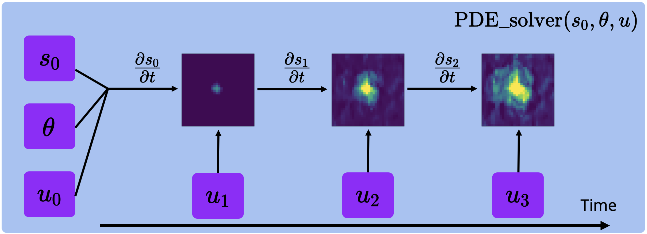
The standard approach to hydrodynamic simulation is to apply the finite-difference (or finite-volume) method to a set of partial differential equations (PDE) of multi-phase flow through a porous medium. Let $\theta$ represent static reservoir variables (computational grid, initial permeability and porosity fields, etc.). Reservoir state at time $t$ will be denoted as $s(t)$ and contain pore pressure, gas content, oil, water and gas saturations. Let also denote production and injection schedules at time $t$ as $u(t)$ and call them control variables. In the classical simulation, the control variable can be defined in many ways. We will assume it contains bottomhole pressures for all production wells and injection rates for all injection wells (at time $t$). The output of the simulation at time $t$ is the state at the next time step $s(t+\Delta t)$. Thus, one step of the standard simulation process can be described as

$$s(t+\Delta t)=\textrm{PDE\_solver}(s(t),u(t),\theta,\Delta t)\,.$$ (1)

The example of classical hydrodynamic simulation with the finite-differences method is shown in Fig. 1. Now we move to description of the proposed model.

Figure 1: Classical simulation scheme with the finite-differences method. Here $\theta$, $s_{0}$ and $u_{i}$ denote reservoir static variables, initial state and control parameters for the time interval. At each timestep the simulation process (1) outputs the solution $s_{i}$ and we show only some slices of the 3D cubes obtained.

2.1 Latent space dynamics

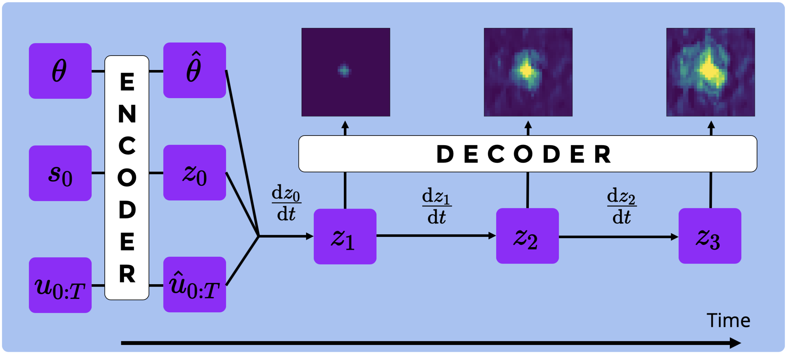
The proposed reservoir simulation model is inspired by the Reduced Order Modelling (ROM) technique presented in Kani and Elsheikh (2018) and recently applied e.g. in Jin et al. (2020) and the Neural Ordinary Differential Equations (neural ODEs) introduced in Chen et al. (2018). For brevity we call the model Neural Differential Equations based Reduced Order Model (NDE-b-ROM). The idea is to translate the reservoir dynamics into a latent space using encoder-decoder NNs and reconstruct latent space dynamics using differentiable neural ODE. This gives a more flexible approach in contrast to linear decomposition models (e.g. Dynamic Mode Decomposition (Kutz et al., 2016)) and can be compared to several non-linear models based on NNs proposed in Temirchev et al. (2020); Watter et al. (2015); Banijamali et al. (2017).

More precisely, we approximate reservoir dynamics in a space of compressed (latent) reservoir state representations $z(t)$. In the following description we will use bold letters (e.g. $\bf g$, $\bf E_{\theta}$) to indicate functions that are unknown a priory and are specified during the model training stage. Of course, after the model is trained, these functions are considered as completely defined. Thus we assume an existence of mappings ${\bf E_{s}}:\mathcal{S}\rightarrow\mathcal{Z}$ and ${\bf E_{z}}:\mathcal{Z}\rightarrow\mathcal{S}$ between full-order states and its latent representations such that the composition ${\bf E_{z}}\circ{\bf E_{s}}$ is close to the identical operator. Latent space dynamics is assumed to be governed by an ODE of the form:

$$\frac{dz}{dt}={\bf g}(z(t),\hat{u}(t),\hat{\theta})\,,$$ (2)

were ${\bf g}(\cdot)$ is some non-linear function, $\hat{u}$ and $\hat{\theta}$ represent latent control and latent static variables of an oilfield. Latent control and static variables are assumed to be obtained from mappings ${\bf E_{u}}:\mathcal{U}\rightarrow\hat{\mathcal{U}}$ and ${\bf E_{\theta}}:\Theta\rightarrow\hat{\Theta}$ respectively.

The simulation process starts with an initial reservoir state $s(0)$ and requires well control schedule $u(t)$ and static information $\theta$. The next reservoir states $s(t)$ are obtained iteratively as follows::

• Encode initial state $z(0)={\bf E_{s}}(s(0))$, static variables $\hat{\theta}={\bf E_{\theta}(\theta)}$ and control $\hat{u}(t)={\bf E_{u}}(u(t))$ for all $t$;

• Solve the latent ODE for a required period of time using any appropriate numerical scheme. For example, using an explicit integration scheme: $z(t+\Delta t)=z(t)+\Delta t\cdot{\bf g}(z(t),\hat{u}(t),\hat{\theta})$. As a result we obtain the latent solution $z(t)$ for all $t$;

• Decode the latent solution: $s(t)={\bf E_{z}}(z(t))$ for all $t$.

The overall structure of the proposed process is presented in Fig. 2.

Figure 2: Simulation scheme with the NDE-b-ROM model. Here $\theta$, $s_{0}$ and $u_{0:T}$ denote reservoir static variables, initial state and control parameters for the time interval $(0:T)$. These variables pass through the encoder (which is specific for each variable) and are mapped into the latent space variables denoted as $\hat{\theta}$, $z_{0}$ and $\hat{u}_{0:T}$. Solving the ODE (2) in the latent space we obtain a set of latent solutions $z_{1}$, $z_{2}$, etc. Decoding latent states $z_{i}$ we obtain a solution in the initial space and show only some slices of the 3D cubes obtained.

2.2 Neural Network Architecture

The introduced mappings $\bf E_{s}$, $\bf E_{z}$ $\bf E_{u}$, $\bf E_{\theta}$ and $\bf g$ are represented by fully-convolutional NNs (Long et al., 2015). A benefit of the fully-convolutional architecture is a natural scalability of the model. In the context of reservoir simulation it allows processing of oil fields of different sizes.

Mappings $\bf E_{s}$, $\bf E_{u}$, $\bf E_{\theta}$ (encoders) are approximated by 4-layer fully-convolutional NNs. The dimensionality reduction is controlled by the stride parameter of convolutions. The mapping $\bf E_{z}$ (decoder) is approximated by a similar NN without strides. Instead, the decoder should increase the dimensionality of a latent variable. It is achieved by the use of a 3-D analog of the Pixel Shuffle method (Shi et al., 2016) (we call it Voxel Shuffle). The function $\bf g$ is approximated by a simple 2-layer convolutional network. All the modules use Batch Normalization (Ioffe and Szegedy, 2015) and Leaky ReLU non-linearity (Maas, 2013). This architecture is a result of the compromise between the model depth and ability to fit into a limited GPU memory when training on large reservoir models with a large number of timestamps. Of course, there are many internal parameters in each layer that might require specification. In order to provide the full reproducibility on the model we open-source the code of the model as well as any details of data processing and model training steps in the GitHub repository https://github.com/Skoltech-CHR/DeepField.

It should be also noted that in contrast to the standard downscaling-upscaling procedures we do not expect substantial information leakage about reservoir heterogeneities in the latent space. The point is that during the model training stage the encoder-decoder pairs are optimized in a way that their composition acts as the identity transform.

2.3 Training procedure

NDE-b-ROM is trained end-to-end in a supervised manner. This requires to have a training dataset $\mathcal{D}$ that gives examples of true dynamics evolution.

In supervised learning, dataset comprises a set of pairs $\{X_{i},Y_{i}\}_{i=0}^{N}$. Here $X_{i}$ is known information about $i$-th reservoir:

$$X_{i}=\{s_{i}(0),\theta_{i},u_{i}(0),u_{i}(t_{1}),u_{i}(t_{2}),\dots\}\,,$$ (3)

while $Y_{i}$ is a target containing all the information that should be predicted by a model:

$$Y_{i}=\{s_{i}(t_{1}),s_{i}(t_{2}),s_{i}(t_{3}),\dots\}\,,$$ (4)

and $N$ is the dataset size.

Commonly, datasets of sufficient size are not available due to technical and commercial subtleties. To overcome this problem we take several hydrodynamic models of real oilfields, randomize them and perform simulation of state (target) variables using classical reservoir simulators. Randomization is made in two steps:

• Create new initial state and static variables by adding a small amount of correlated zero-mean Gaussian noise. Create a new bottomhole pressure schedule by sampling from some distribution (see the discussion below). This step generates $X_{i}$.

• Feed the generated initial data into a classical finite difference hydrodynamic simulator and get true dynamics $Y_{i}$.

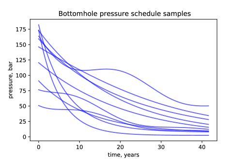
The choice of good generative schemes is a non-trivial problem and requires a separate investigation. For simplicity, we applied Gaussian randomization for static variables and initial states. We use correlated noise in order to vary large-scale field properties rather than to simulate even larger uncertainties about values in particular grid cells. For bottomhole pressure a hand-crafted scheme was used:

$$u_{i}(t)=\varepsilon_{0}\frac{1-sin(\varepsilon_{1}t+\varepsilon_{2})}{2}\exp(-\varepsilon_{3}t)+\varepsilon_{4}+\varepsilon_{5}(t)\,.$$ (5)

Here $\{\varepsilon_{i}\}_{i=0}^{5}$ are random numbers from a uniform distribution; $\varepsilon_{5}$ is the only component which is resampled at each time step.

Proposed generative scheme gives us realistic initial and boundary conditions as well as a bottomhole pressure schedule (see Fig. 3).

Figure 3: Example of the bottom-hole pressure schedule samples from the generative model.

3 Rates module

Inflow from the cell connected with perforated well segment is calculated on the basis of standard relation between inflow and pressure drop:

$$q_{P}^{l}(t)=C^{l}(t)m^{l}_{P}(t)\left(p^{l}(t)-p^{l}_{con}(t)\right)\,.$$ (6)

Here $q_{P}^{l}(t)$ is a volumetric inflow of a phase $P$ from the $l$-th cell to the well at time $t$, $C^{l}$ denotes connection productivity index, $m^{l}_{P}$ is total mobility of the phase $P$, $p^{l}$ – pressure in the $l$-th cell, $p^{l}_{con}$ – pressure on the well-cell interface.

In case of well parallel to one of the coordinate axis, connection productivity index are calculated explicitly. First we find the effective value of the product of formation permeability $K$ and formation thickness $h$:

$$(Kh)^{l}=\sqrt{k^{l}_{1}k^{l}_{2}}h^{l}\;,$$ (7)

here $k^{l}_{1}$, $k^{l}_{2}$ are permeabilities in the directions perpendicular to the well, $h^{l}$ is length of perforated well segment in the $l$-th cell. Then for the connection index we have

$$C^{l}=\frac{2\pi(Kh)^{l}}{\mathrm{\ln}(r^{l}_{o}/r_{w})}\;,$$ (8)

where $r_{o}$ is equivalent radius (Peaceman radius, Peaceman (1978)), $r_{w}$ is a well radius. Equivalent radius $r_{0}$ is calculated as

$$r^{l}_{0}=0.28\frac{\left((d^{l}_{1})^{2}\left(\frac{k^{l}_{2}}{k^{l}_{1}}\right)^{\frac{1}{2}}+(d^{l}_{2})^{2}\left(\frac{k^{l}_{1}}{k^{l}_{2}}\right)^{\frac{1}{2}}\right)^{\frac{1}{2}}}{\left(\frac{k^{l}_{2}}{k^{l}_{1}}\right)^{\frac{1}{4}}+\left(\frac{k^{l}_{1}}{k^{l}_{2}}\right)^{\frac{1}{4}}}\;,$$ (9)

where $d^{l}_{1}$, $d^{l}_{2}$ denote sizes of $l$-th block in directions perpendicular to the well.

If a well has arbitrary trajectory it is approximated as a piecewise linear one; for each linear segment projection onto coordinate axis are calculated and connection productivity indices are calculated separately for each projections. Thus we obtain projections of the connectivity index onto coordinate index $C^{l}_{x}$, $C^{l}_{y}$, $C^{l}_{z}$. To obtain a resulting connectivity index for the cell we summarize these indices:

$$C^{l}=C^{l}_{x}+C^{l}_{y}+C^{l}_{z}.$$ (10)

The described scheme of rates calculation as well as the dynamics modules are implemented using PyTorch framework (Paszke et al., 2019). This enables automatic gradient propagation through rate calculations and makes it suitable for optimization problems such as history matching.

4 Adaptation scheme

Implementing reservoir simulation model as an end-to-end differentiable neural network, any set of model parameters can be considered as a space for adaptation. Moreover, standard adaptation goal (minimization of a difference between simulated and observed data) can be naturally extended with regularization terms that, e.g., penalize material-balance violation or correction amplitudes. A detailed investigation of various sets of parameters in combination with regularization terms should be a matter of separate research, in this paper we present rather proof-of-concept results and discuss further research options.

Following a common HM approach we consider adaptation in the space of rock parameters (porosity and permeability) and extend it with the auxiliary space of connection productivity indices. Gradient backpropagation through the neural network model allows sensitivity estimation for each individual grid cell block. To avoid the undesired overfitting, we require that changes in a cell block should be correlated with neighboring blocks and penalize large amplitudes using $L_{2}$ regularization. Up to some extent this regularization hinders the capability of the neural network to model various faults. However, providing the model with an additional 3D tensor describing the distribution of fault should help to take this information into account. We attribute this investigation to future research.

Technically, we split initial grid into small cubes of four cell blocks in each direction (of course, one can vary cube sizes to perform adaptation at different spatial scales). Each cube attributes to a single additive rock correction factor, initialized with small-amplitude zero mean random noise (we found this initialization works better than constant zero initialization). These correction factors will be adjusted during HM and propagate back to cell blocks of the initial grid through bilinear upsampling.

To include connectivity indices in a space of adaptation parameters we multiply (6) by additional connectivity correction factors. In order to ensure that connectivity correction factors remain non-negative during adaptation, we will vary its logarithms instead of the connectivity correction factors itself. Logarithms are initialized again with small-amplitude zero mean random noise.

The adaptation process works as follows. We iteratively pass the adaptation time interval with time steps of a fixed size. At each step, we calculate predicted production rates and calculate a loss function that penalties a difference between predicted and target values. Based on the loss function value, we compute gradients with respect to rock and connectivity correction factors and accumulate the gradients. When the time steps reach the end of the adaptation interval, correction factors are updated according to the accumulated gradients and the Adam optimization scheme (Kingma and Ba, 2014). Then the gradients are set to zero, and the next iteration begins.

Figure 4: Adaptation scheme. Orange boxes indicate adaptation variables. Rock correction variables are upscaled to the shape of initial rock variables and are added to them. Then the NDE-b-ROM model computes production rates for each well block. Production rates are multiplied by connectivity correction factors. Then total production rates are compared with historical values and loss function is computed. Using the loss function value gradients are propagated back to adaptation variables. Blue arrows show forward data flow, orange arrows show gradients flow.

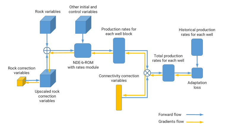
Total loss function at each iteration is defined as the aggregated loss over all steps. Iterations stop when the total loss stops to decrease substantially. Running the model several times and varying parameters of the Adam optimization algorithm, we find that increasing of learning rate to 0.3 provides better and faster convergence. Also, the weight decay parameter is set to $5\times 10^{-4}$, which penalizes large amplitudes of correction factors.

5 Reservoir model

For numerical experiments we used a synthetic model of the one of Western Siberia oilfield. The model grid is represented in corner point geometry with $145\times 121\times 210$ cells, about 1.3M of which are active. In the Fig. 5 structure of the model as well as porosity distribution are presented. Fig. 6 shows oil and gas saturation distributions.

Figure 5: Porosity distribution in the reservoir model.

(a)

(b)

Figure 6: LABEL:sub@fig:saturation:soil – oil saturation distribution, LABEL:sub@fig:saturation:sgas – gas saturation distribution in the reservoir model.

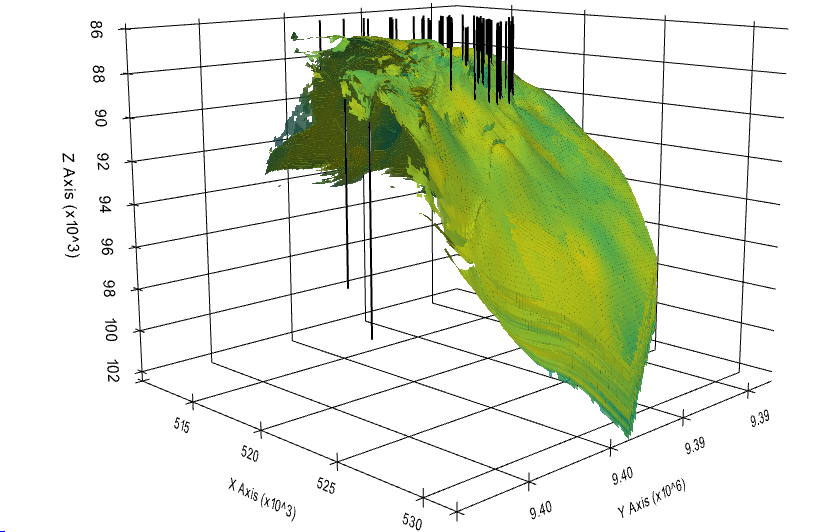
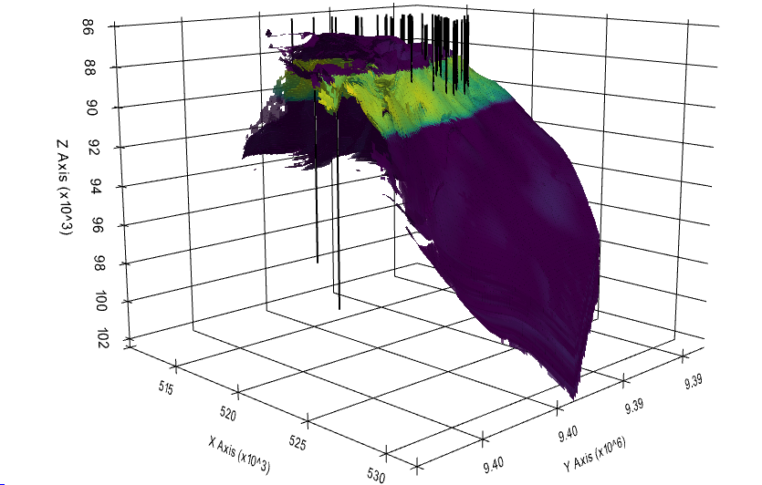
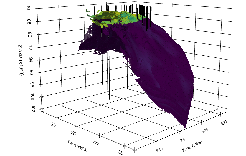
The oilfield has anticlinal shape with gas cap in the top and oil fringe under the gas cap. The complex structure of the model with both gas cap and underlying water make it very sensitive to modelling accuracy. The simulator has to be capable of proper simulation of water and gas coning effects.

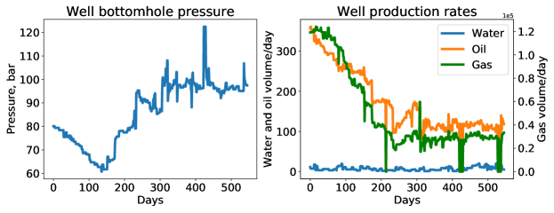
The hydrocarbons are recovered with the use of 64 production wells located in both oil and gas areas. Due to the early stage of reservoir recovery, only a small fraction of wells has more or less complete production history. We carefully selected a time interval and a set of wells involved in this research to eliminate low-quality records and, in particular, to eliminate wells with only fragmentary history available. The reason for this preprocessing is as follows. It is clear that data quality is essential for accuracy of adaptation results. However, it is rather difficult to separate the impact of data quality and model capability itself. The aim of this paper is to demonstrate the generic approach, while application to different reservoir models with specifically complicated history data might require a customization of data preprocessing steps. The latter discussion is out of the scope of this paper. Finally, we use a set of 12 wells and a time interval of 1.5 years. Each well has daily recorded historical oil, water and gas production rates as well as bottomhole pressure. The recorded bottomhole pressure is used as control parameter in reservoir simulation. An example of recorded history for one of the wells is presented in the Fig. 7.

Figure 7: Historical recorded bottomhole pressure (left panel) and production rates (right panel) for a sample well. Note the double axis (one for water and oil volumes and one for gas volume) in the right panel.

6 Results

In this section, we provide results of an experiment in which rock parameters are varied on a grid downsampled by factor 4 with respect to original grid sizes. Note that downsampling is applied not due to resource limitation but as a natural regularization for HM. The loss function for HM is defined as mean squared error (MSE) between predicted and historical (target) rates for each well and aggregated over all wells and fluid phases (gas, water, oil). To normalize substantially different scales in production rates of various fluid phases, we apply logarithmic calibration before computing the MSE. Also, we apply a linear time-weighting function that increases an impact of error with time progressing. An intuition behind this weighting is that errors in recent rates are more important in comparison to more time-remote errors.

Fig. 8 shows the total loss function decrease against iterations. After 150 iterations loss stops to decrease and begins to fluctuate near a constant value. We stop the adaptation process at this moment.

Figure 8: Adaptation loss function decay against iterations.

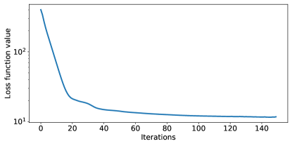
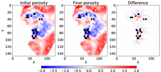
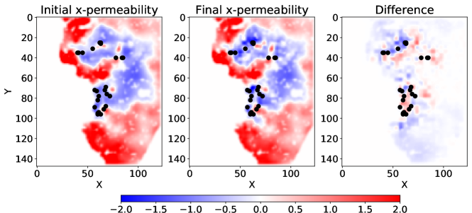
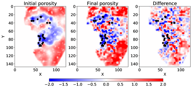
Fig. 9 and Fig. 10 show a sample horizontal slice of the cube of normalized porosity and x-permeability. Note that due to weight regularization the adaptation process affects only a small region around the production wells. In contrast, a model without regularization makes changes even in areas remote from production wells, which is less physically sound (see Fig. 11 for comparison).

Figure 9: Sample horizontal slice of the cube of normalized porosity values. The left panel shows the initial porosity distribution. The middle panel is the result of adaptation. The right panel shows the difference between the plots. Black dots indicate the location of production wells. Weights regularization is applied during adaptation.

Figure 10: Same as Fig. 9 but for the cube of normalized x-permeability.

Figure 11: Same as Fig. 9 but without weights regularization during adaptation.

The next Fig. 15 shows how much are the changes in adaptation parameters introduced by the HM. On average, rock variables obtain a small negative bias -0.01 (significant statistically). However, we find that the initial phase content (i.e. porosity multiplied by phase saturation and cell volume) changes only by less than $1\%$. Quite interesting, we find that almost all connectivity correction factors are distributed near 0 and 1 (being unit initialized). Since the connectivity correction factor is multiplicative, value 1 means no correction is applied, while 0 corresponds to a effectively closed cell’s perforation. Note that this result requires a separate detailed investigation in order to avoid physically irrelevant situations when e.g. several well’s block are substituted with a single block of increased connectivity index. We admit that additional regularization terms might be proposed to control the distribution of connectivity correction factors.

Figure 12: Distribution of rock (left panel) and connectivity (right panel) correction factors. Note that rock corrections are additive, while connectivity corrections are multiplicative. Red line in the left plot shows the mean value of the distribution.

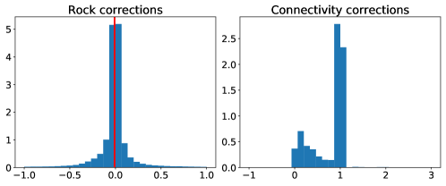
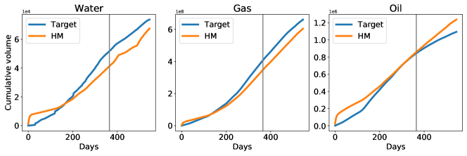
Fig. 13 shows a comparison of target and simulated cumulative production rates. Note that the time interval is split into two parts. The first one shows a comparison within the adaptation period. The second one demonstrates a prediction against historical values. We observe that the model is possible to reproduce the historical values given in the adaptation period and can be used for forecasting on an interval that is at least half of the adaptation period length. The same plot but for a sample well is shown in Fig. 14. We observe that predicted values partially go off-track, e.g. for the water. We address this issue to the current limitation of the neural network model that supports only the limited scope of features and events given in the reservoir history data. More detailed technical description is available in the documentation that supports the open-sourced code.

Figure 13: Cumulative production rates over all wells. Blue line shows historical values, orange line is a model simulation. Vertical line separates adaptation and prediction periods.

Figure 14: Cumulative production rates for a sample well. Blue line shows historical values, orange line is a model simulation. Vertical line separates adaptation and prediction periods. Note that daily historical rates and borehole pressure for the same well are shown in Fig. 7.

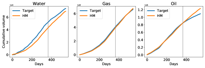
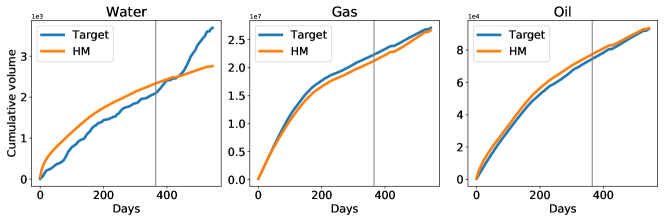
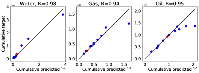
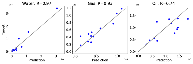
Fig. 15 shows a correlation diagram between predicted and target cumulative production rates over all wells. We observe that for each phase (water, gas, and oil), the correlation coefficient ($R$ value) is 0.94 or above. This indicates that the adaptation process successfully matches the production rates of individual wells.

Figure 15: Correlation between target and predicted cumulative production rates for individual wells (shown as dots). Correlation coefficients are given in the title of each plot. Inclined gray line corresponds to $R=1$. Well shown in red is the same well as in Fig. 14 and Fig. 7.

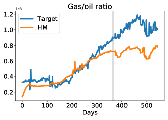
In Fig. 16 we provide a gas/oil a ratio computed according to daily simulated and historical gas and oil production rates. Since the gas/oil ratio is a critical parameter in the reservoir recovery management, we find that predicted values are in partial agreement with actual historical values.

Figure 16: Gas/oil ratio according to daily gas and oil production rates. Blue line shows target (historical) values, orange line is a simulation. Vertical line separates adaptation and prediction intervals.

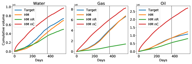
To demonstrate the role of rock and connectivity correction factors, we exclude from simulation either rock or connectivity correction factors and compare the simulation with target values and a simulation where both factors are included. One can note in Fig. 17 that each set of adaptation variables is meaningful, and its combination gives substantially better results.

Figure 17: Cumulative production rates aggregated over all wells. Target (blue line) shows historically recorded values. The orange line (labeled "HM") is a model simulation. The green line (labeled "HM nR") shows a model simulation where rock correction factors are not applied. The red line (labeled "HM nC") shows a model simulation where connectivity correction factors are not applied.

Finally, we demonstrate that adaptation only in the space of rock correction factors (without including connectivity factors) limits the model quality. Indeed, while cumulative production rates over all wells shown in Fig. 18 are compatible with previous Fig. 13, correlation between individual wells become substantially worse (compare Fig. 19 and Fig. 15). We conclude that adaptation in the joint space of rock and connectivity factors allows better matching for individual wells. One can also conclude from the last example that for evaluation of different adaptation models total production rates can not be a single benchmark and additional metrics should be considered as well.

Figure 18: Same as Fig 13 but only rock correction factors were varied during adaptation.

Figure 19: Same as Fig 15 but only rock correction factors were varied during adaptation.

7 Conclusions

We presented an end-to-end neural network approach that allows reservoir simulation and history matching with standard gradient-based optimization algorithms. The neural network model has initial geological parameters of the 3D reservoir model in the input. In the output, the model returns wells’ production rates. By construction, neural network models allow gradients propagation to any internal and input variables. Using a dataset of development scenarios, we train the neural network to simulate general geological relations. In this case, internal network variables are optimized. Using historical records on real production rates and bottomhole pressure, we solve the history matching problem. In this case, initial rock parameters and connectivity indices were optimized. As we demonstrated, the final model allows reliable simulation of historical production rates and forecasting of reservoir dynamics.

It should be noted that the suggested neural network approach is not to replace standard industrial reservoir simulation software. The goal is to obtain a substantially faster simulation tool, probably at the cost of acceptable accuracy decrease. In this research, we consider the reservoir model of about 3.7M total grid cell size and about 1.3M of active cells. Simulation of daily production rates for 1.5 years time interval takes about 1 minute (using modern GPU workstation). Note that the computation also includes a complete simulation of pressure and phase saturation cubes. This result is several orders of magnitude faster in comparison to current industrial reservoir simulation software. The adaptation process for one-year period takes about 3 hours.

The neural network approach opens a broad and convenient way for implementation of many reservoir simulation and adaptation strategies. The point is that one can easily combine variables to be optimized during HM. For example, in this research, we consider a joint adaptation in the space of rock parameters and connectivity indices. Also, the HM and forward simulation problems can be naturally extended by additional regularization terms, including a control for proper conservation of physical parameters such as mass of components. Investigation and comparison of the various experiment settings is a matter of future research, which looks optimistic taking into account proof-of-the-concept results demonstrated in this paper.

This research is completely based on the source-code available in the GitHub repository https://github.com/Skoltech-CHR/DeepField.

References

- Banijamali et al. (2017) Banijamali, E., Shu, R., Ghavamzadeh, M., Bui, H.H., Ghodsi, A., 2017. Robust locally-linear controllable embedding. CoRR abs/1710.05373. URL: http://arxiv.org/abs/1710.05373, arXiv:1710.05373.
- Chen et al. (2018) Chen, T.Q., Rubanova, Y., Bettencourt, J., Duvenaud, D.K., 2018. Neural ordinary differential equations. CoRR abs/1806.07366. URL: http://arxiv.org/abs/1806.07366, arXiv:1806.07366.
- Chen et al. (2006) Chen, Z., Huan, G., Ma, Y., 2006. Computational Methods for Multiphase Flows in Porous Media. Society for Industrial and Applied Mathematics. URL: http://epubs.siam.org/doi/book/10.1137/1.9780898718942, doi:10.1137/1.9780898718942.
- Goodfellow et al. (2016) Goodfellow, I., Bengio, Y., Courville, A., 2016. Deep Learning. MIT Press. http://www.deeplearningbook.org.
- Gómez et al. (2001) Gómez, S., Gosselin, O., Barker, J., 2001. Gradient-based history matching with a global optimization method. SPE Journal - SPE J 6, 200--208. doi:10.2118/71307-PA.
- Illarionov et al. (2020) Illarionov, E., Temirchev, P., Voloskov, D., Gubanova, A., Koroteev, D., Simonov, M., Akhmetov, A., Margarit, A., 2020. 3d reservoir model history matching based on machine learning technology. URL: https://doi.org/10.2118/201924-MS, doi:10.2118/201924-MS. d023S012R001.
- Ioffe and Szegedy (2015) Ioffe, S., Szegedy, C., 2015. Batch normalization: Accelerating deep network training by reducing internal covariate shift. CoRR abs/1502.03167. URL: http://arxiv.org/abs/1502.03167, arXiv:1502.03167.
- Jin et al. (2020) Jin, Z.L., Liu, Y., Durlofsky, L.J., 2020. Deep-learning-based surrogate model for reservoir simulation with time-varying well controls. Journal of Petroleum Science and Engineering 192, 107273. URL: https://www.sciencedirect.com/science/article/pii/S0920410520303533, doi:https://doi.org/10.1016/j.petrol.2020.107273.
- Kaleta et al. (2011) Kaleta, M., Hanea, R., Heemink, A., Jansen, J.D., 2011. Model-reduced gradient-based history matching. Computational Geosciences 15, 135--153. doi:10.1007/s10596-010-9203-5.
- Kani and Elsheikh (2018) Kani, J.N., Elsheikh, A.H., 2018. Reduced order modeling of subsurface multiphase flow models using deep residual recurrent neural networks. CoRR abs/1810.10422.
- Kingma and Ba (2014) Kingma, D.P., Ba, J., 2014. Adam: A Method for Stochastic Optimization. arXiv e-prints , arXiv:1412.6980arXiv:1412.6980.
- Koroteev and Tekic (2021) Koroteev, D., Tekic, Z., 2021. Artificial intelligence in oil and gas upstream: Trends, challenges, and scenarios for the future. Energy and AI 3, 100041. URL: http://www.sciencedirect.com/science/article/pii/S2666546820300410, doi:https://doi.org/10.1016/j.egyai.2020.100041.
- Kutz et al. (2016) Kutz, J.N., Brunton, S.L., Brunton, B.W., Proctor, J.L., 2016. Dynamic Mode Decomposition. Society for Industrial and Applied Mathematics, Philadelphia, PA. URL: https://epubs.siam.org/doi/abs/10.1137/1.9781611974508, doi:10.1137/1.9781611974508, arXiv:https://epubs.siam.org/doi/pdf/10.1137/1.9781611974508.
- Kvashchuk et al. (2019) Kvashchuk, A., Klöfkorn, R., Sandve, T.H., 2019. Comparison of higher order schemes on complicated meshes and reservoirs. URL: https://doi.org/10.2118/193839-MS, doi:10.2118/193839-MS. d011S005R002.
- Long et al. (2015) Long, J., Shelhamer, E., Darrell, T., 2015. Fully convolutional networks for semantic segmentation. arXiv:1411.4038.
- Maas (2013) Maas, A.L., 2013. Rectifier nonlinearities improve neural network acoustic models.
- Oliver and Chen (2011) Oliver, D.S., Chen, Y., 2011. Recent progress on reservoir history matching: a review. Computational Geosciences 15, 185--221. URL: https://doi.org/10.1007/s10596-010-9194-2, doi:10.1007/s10596-010-9194-2.
- Paszke et al. (2019) Paszke, A., Gross, S., Massa, F., Lerer, A., Bradbury, J., Chanan, G., Killeen, T., Lin, Z., Gimelshein, N., Antiga, L., Desmaison, A., Kopf, A., Yang, E., DeVito, Z., Raison, M., Tejani, A., Chilamkurthy, S., Steiner, B., Fang, L., Bai, J., Chintala, S., 2019. Pytorch: An imperative style, high-performance deep learning library, in: Wallach, H., Larochelle, H., Beygelzimer, A., d'Alché-Buc, F., Fox, E., Garnett, R. (Eds.), Advances in Neural Information Processing Systems 32. Curran Associates, Inc., pp. 8024--8035. URL: http://papers.neurips.cc/paper/9015-pytorch-an-imperative-style-high-performance-deep-learning-library.pdf.
- Peaceman (1978) Peaceman, D.W., 1978. Interpretation of well-block pressures in numerical reservoir simulation , 17.
- Shi et al. (2016) Shi, W., Caballero, J., Huszár, F., Totz, J., Aitken, A.P., Bishop, R., Rueckert, D., Wang, Z., 2016. Real-time single image and video super-resolution using an efficient sub-pixel convolutional neural network. arXiv:1609.05158.
- Sun and Zhang (2020) Sun, S., Zhang, T., 2020. Reservoir Simulation: Machine Learning and Modeling. Elsevier. URL: https://www.sciencedirect.com/book/9780128209578/reservoir-simulations, doi:10.1016/C2019-0-02019-5.
- Temirchev et al. (2020) Temirchev, P., Simonov, M., Kostoev, R., Burnaev, E., Oseledets, I., Akhmetov, A., Margarit, A., Sitnikov, A., Koroteev, D., 2020. Deep neural networks predicting oil movement in a development unit. Journal of Petroleum Science and Engineering 184, 106513. URL: http://www.sciencedirect.com/science/article/pii/S0920410519309349, doi:https://doi.org/10.1016/j.petrol.2019.106513.
- Watter et al. (2015) Watter, M., Springenberg, J.T., Boedecker, J., Riedmiller, M.A., 2015. Embed to control: A locally linear latent dynamics model for control from raw images, in: NIPS.