Towards Accurate and Compact Architectures via Neural Architecture Transformer

Abstract

Designing effective architectures is one of the key factors behind the success of deep neural networks. Existing deep architectures are either manually designed or automatically searched by some Neural Architecture Search (NAS) methods. However, even a well-designed/searched architecture may still contain many nonsignificant or redundant modules/operations (e.g., some intermediate convolution or pooling layers). Such redundancy may not only incur substantial memory consumption and computational cost but also deteriorate the performance. Thus, it is necessary to optimize the operations inside an architecture to improve the performance without introducing extra computational cost. To this end, we have proposed a Neural Architecture Transformer (NAT) method which casts the optimization problem into a Markov Decision Process (MDP) and seeks to replace the redundant operations with more efficient operations, such as skip or null connection. Note that NAT only considers a small number of possible transitions and thus comes with a limited search/transition space. As a result, such a small search space may hamper the performance of architecture optimization. To address this issue, we propose a Neural Architecture Transformer++ (NAT++) method which further enlarges the set of candidate transitions to improve the performance of architecture optimization. Specifically, we present a two-level transition rule to obtain valid transitions, i.e., allowing operations to have more efficient types (e.g., convolution${\to}$separable convolution) or smaller kernel sizes (e.g., $5{\times}5{\to}3{\times}3$). Note that different operations may have different valid transitions. We further propose a Binary-Masked Softmax (BMSoftmax) layer to omit the possible invalid transitions. Last, based on the MDP formulation of NAT and NAT++, we apply policy gradient to learn an optimal policy, which will be used to infer the optimized architectures. We apply NAT and NAT++ to optimize both hand-crafted architectures and NAS based architectures. Extensive experiments on several benchmark datasets show that the transformed architecture significantly outperforms both its original counterpart and the architectures optimized by existing methods.

1 Introduction

Deep neural networks (DNNs) [1] have produced state-of-the-art results in many challenging tasks including image classification [2, 3, 4, 5, 6, 7], face recognition [8, 9, 10], and object detection [11, 12, 13]. One of the key factors behind the success lies in the innovation of neural architectures, such as VGG [14] and ResNet[15]. However, designing effective neural architectures is often very labor-intensive and relies heavily on human expertise. More critically, such a human-designed process is hard to fully explore the whole architecture design space. As a result, the resultant architectures are often very redundant and may not be optimal. Hence, there is a growing interest in replacing the manual process of architecture design with an automatic way called Neural Architecture Search (NAS).

Recently, substantial studies [16, 17, 18, 19] have shown that automatically discovered architectures are able to achieve highly competitive performance compared to the hand-crafted architectures. However, there are some limitations to the NAS based architecture design methods. In fact, since there is an extremely large search space [17, 18] (e.g., billions of candidate architectures), these methods are hard to be trained and often produce sub-optimal architectures, leading to the limited representation performance or substantial computational cost. Thus, even for the architectures searched by NAS methods, it is still necessary to optimize their redundant operations to achieve better performance and/or reduce the computational cost.

To optimize the architectures, Luo et al. recently proposed a Neural Architecture Optimization (NAO) method [20]. Specifically, NAO first encodes an architecture into an embedding in the continuous space and then conducts gradient descent to obtain a better embedding. After that, it uses a decoder to map the embedding back to obtain an optimized architecture. However, NAO has its own set of limitations. First, NAO often produces a totally different architecture from the input architecture, making it hard to analyze the relationship between the optimized and the original architectures (See Fig. 1). Second, NAO may improve the architecture design at the expense of introducing extra parameters or computational cost. Third, similar to the NAS methods, NAO has a very large search space, which may not be necessary for architecture optimization and may make the optimization problem very expensive to solve. An illustrative comparison between our methods and NAO can be found in Fig. 1.

Figure 1: Comparison between Neural Architecture Optimization (NAO) [20] and our Neural Architecture Transformer (NAT). Green blocks denote the two input nodes of the cell and blue blocks denote the intermediate nodes. Red blocks denote the connections that are changed by NAT. The accuracy and the number of parameters are evaluated on CIFAR-10 models.

Unlike existing methods that design/find neural architectures, we have proposed a Neural Architecture Transformer (NAT) [21] method to automatically optimize neural architectures to achieve better performance and/or lower computational cost. To this end, NAT replaces the expensive operations or redundant modules in an architecture with the more efficient operations. Note that NAT can be used as a general architecture optimizer that takes any architecture as input and outputs an optimized architecture. NAT has shown great performance in optimizing various architectures on several benchmark datasets. However, NAT only considers three operation transitions, i.e., remaining unchanged, replacing with null connection, replacing with skip connection. Such a small search/transition space may hamper the performance of architecture optimization. Thus, it is important and necessary to enlarge the search space of architecture optimization.

In this paper, based on NAT, we propose a Neural Architecture Transformer++ (NAT++) method which considers a larger search space to conduct architecture optimization in a finer manner. To this end, we present a two-level transition rule to simultaneously change both the type and the kernel size of an operation in architecture optimization. Specifically, NAT++ encourages operations to have more efficient types (e.g., convolution${\to}$separable convolution) or smaller kernel sizes (e.g., $5{\times}5{\to}3{\times}3$). For convenience, we use valid transitions to denote those transitions that do not increase the computational cost. Note that different operations may have different valid transitions. To make NAT++ accommodate all the considered operations, we propose a Binary-Masked Softmax (BMSoftmax) layer to omit all the invalid transitions that violate the transition rule. In this way, NAT++ is able to predict the optimal transitions for the operations with different valid transitions simultaneously. Extensive experiments show that our NAT++ significantly outperforms existing methods.

The contributions of this paper are summarized as follows.

• We propose a Neural Architecture Transformer (NAT) method which optimizes arbitrary architectures for better performance and/or less computational cost. To this end, NAT either removes the redundant operations or replaces them with skip connections. To better exploit the adjacency information of operations in an architecture, we propose to exploit graph convolutional network (GCN) to build the architecture optimization model.

• Based on NAT, we propose a Neural Architecture Transformer++ (NAT++) method which considers a larger search space for architecture optimization. Specifically, NAT++ presents a two-level transition rule which encourages operations to have a more efficient type and/or a smaller kernel size. Thus, NAT++ is able to automatically obtain the valid transitions (i.e., the transitions to more efficient operations).

• To accommodate the operations which may have different valid transitions, we propose a Binary-Masked Softmax (BMSoftmax) layer to build a general NAT++ model which predicts the optimal transitions for all the operations simultaneously.

• Extensive experiments on several benchmark datasets show that our NAT and NAT++ consistently improve the design of various architectures, including both hand-crafted and NAS based architectures. Compared to the original architectures, the optimized architectures tend to yield significantly better performance and/or lower computational cost.

This paper extends our preliminary version [21] from several aspects. 1) We propose an advanced version NAT++ by enlarging the search space to improve the performance of architecture optimization. 2) We present a two-level transition rule to automatically obtain the valid transitions for each operation on both the operation type level and the kernel size level. 3) We propose a Binary-Masked Softmax (BMSoftmax) layer to omit all the invalid transitions. 4) We compare the computational cost of different operations and analyze the effect of the transitions among them on our method. 5) We provide more analysis about the impact of different operations on the convergence speed of architectures. 6) We investigate the possible bias towards the architectures with too many skip connections in the proposed method. 7) We provide more empirical results to show the effectiveness of NAT and NAT++ based on various architectures.

Figure 2: An example of the graph representation of a residual block and the diagram of operation transformations. (a) a residual block [15]; (b) a graph view of residual block; (c) transitions among three kinds of operations. ${N}$ denotes a null operation without any computation, ${S}$ denotes a skip connection, and ${O}$ denotes some computational modules other than null and skip connections.

2 Related Work

2.1 Hand-crafted Architecture Design

Many studies have proposed a series of deep neural architectures, such as AlexNet [3], VGG [14] and so on. Based on these models, many efforts have been made to further increase the representation ability of deep networks. Szegedy et al. propose the GoogLeNet [22] which consists of a set of convolutions with different kernel sizes. He et al. propose the residual network (ResNet) [15] by introducing residual shortcuts between different layers. To design more compact models, MobileNet [23, 24] employs depthwise separable convolution to reduce model size and computational overhead. ShuffleNet [25, 26] exploits pointwise group convolution and channel shuffle to significantly reduce computational cost while maintaining comparable accuracy. However, the human-designed process often requires substantial human effort and cannot fully explore the whole architecture space.

2.2 Neural Architecture Search

Recently, neural architecture search (NAS) has been proposed to automate the process of architecture design [27, 28, 29, 30, 31]. Specifically, Zoph et al.  use a recurrent neural network as the controller [18] to construct each convolution by determining the optimal stride, the number and the shape of filters. Pham et al.  propose a weight sharing technique [17] to significantly improve search efficiency. Liu et al.  propose a differentiable NAS method, called DARTS [16], which relaxes the search space to be continuous. Recently, Luo et al. propose the Neural Architecture Optimization (NAO) [20] method to perform architecture search on continuous space by exploiting encoding-decoding technique. Unlike these methods, our method optimizes architectures without introducing extra computational cost (See comparisons in Fig. 1).

2.3 Architecture Adaptation and Model Compression

Several methods have been proposed to adapt architectures to some specific platform or compress some existing architectures. To obtain compact models,  [32, 33, 34, 35] adapt architectures to the more compact ones by learning the optimal settings of each convolution. One can also exploit model compression methods [36, 37, 38, 39] to remove the redundant channels to obtain compact models. Recently, ESNAC [40] uses Bayesian optimization techniques to search for a compressed network via layer removal, layer shrinkage, and adding skip connections. ASP [41] proposes an affine parameter sharing method to search for the optimal channel numbers of each layer to optimize architectures. Nevertheless, these methods have to learn a compressed model for a specific architecture and have limited generalization ability to different architectures. Unlike these methods, we seek to learn a general optimizer for arbitrary architecture.

Figure 3: The scheme of the proposed NAT. Our NAT takes an arbitrary architecture as input and produces the optimized architecture as the output. We use blue arrows to represent the process of architecture optimization. Red arrows and boxes denote the computation of reward and gradients. $R(\alpha|\beta)$ denotes the reward that measures the performance improvement between two architectures $\alpha$ and $\beta$.

3 Neural Architecture Transformer

3.1 Problem Definition

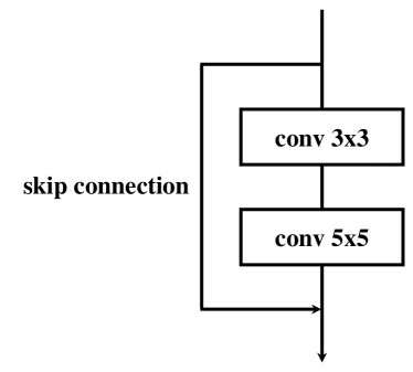
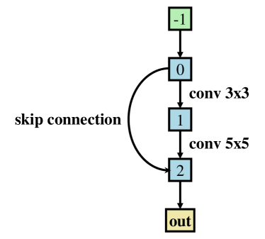
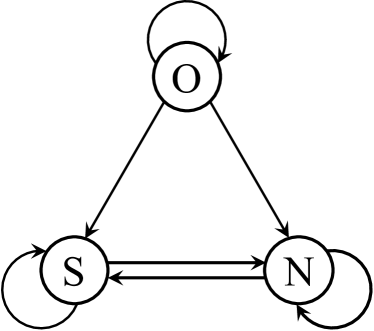
Following [17, 16], we consider a cell as the basic block to build the entire network. Given a cell based architecture space $\Omega$, we can represent an architecture $\alpha$ as a directed acyclic graph (DAG), i.e., $\alpha=\left(\mathcal{V},\mathcal{E}\right)$, where ${\mathcal{V}}$ is a set of nodes that denote the feature maps in DNNs and $\mathcal{E}$ is an edge set [18, 17, 16], as shown in Fig. 2. Here, a DAG contains $|{\mathcal{V}}|$ nodes $\{{\bf X}_{l}\}_{l=-2}^{|{\mathcal{V}}|-3}$, where ${\bf X}_{-2}$ and ${\bf X}_{-1}$ denote the outputs of two previous cells, and ${\bf X}_{|{\mathcal{V}}|-3}$ denotes the output node that concatenates all intermediate nodes $\{{\bf X}_{l}\}_{l=0}^{|{\mathcal{V}}|-3}$. Each intermediate node is able to connect with all previous nodes. The directed edge $e_{ij}\in{\mathcal{E}}$ denotes some operation (e.g., convolution or max pooling) that transforms the feature map from node $v_{i}$ to $v_{j}$. For convenience, we divide the edges in ${\mathcal{E}}$ into three categories, namely, $S$, ${N}$, $O$, as shown in Fig. 2. Here, ${S}$ denotes the skip connection, ${N}$ denotes the null connection (i.e., no edge between two nodes), and ${O}$ denotes the operations other than skip connection or null connection (e.g., convolution or max pooling). Note that different operations have different cost. Specifically, let $c(\cdot)$ be a function to evaluate the computational cost. Obviously, we have $c({O})>c({S})>c({N})$.

In this paper, we propose an architecture optimization method, called Neural Architecture Transformer (NAT), to optimize any given architecture to achieve better performance and/or less computational cost. To avoid introducing extra computational cost, an intuitive way is to make the original operation have less computational cost, e.g., replacing operations with skip or null connection. Although skip connection has a slightly higher cost than null connection, it often can significantly improve the performance [15, 42]. Thus, we enable the transition from null connection to skip connection to increase the representation ability of deep networks. In summary, we constrain the possible transitions among $O$, $S$ and ${N}$ in Fig. 2 in order to reduce the computational cost.

3.2 Markov Decision Process for NAT

In this paper, we seek to learn a general architecture optimizer which takes any given architecture as input and outputs the corresponding optimized architecture. Let $\beta$ be the input architecture which follows some distribution $p(\cdot)$, e.g., multivariate uniformly discrete distribution. We seek to obtain the optimized architecture $\alpha$ by learning the mapping $\alpha\leftarrow{\rm NAT}(\beta;\theta)$, where $\theta$ denotes the learnable parameters. Let $w_{\alpha}$ and $w_{\beta}$ be the well-learned model parameters of architectures $\alpha$ and $\beta$, respectively. We measure the performance of $\alpha$ and $\beta$ by some metric $R(\alpha,w_{\alpha})$ and $R(\beta,w_{\beta})$, e.g., accuracy. For convenience, we define the performance improvement between $\alpha$ and $\beta$ by $R(\alpha|\beta)=R(\alpha,w_{\alpha})-R(\beta,w_{\beta})$. To illustrate our method, we first discuss the architecture optimization problem for a specific architecture and then generalize it to the problem for different architectures.

To learn a good architecture transformer ${\rm NAT}(\beta;\theta)$ to optimize a specific $\beta$, we can maximize the performance improvement $R(\alpha|\beta)$. However, simply maximizing $R(\alpha|\beta)$ may easily find an architecture $\alpha$ with much higher computational cost than the input counterpart $\beta$. Instead, we seek to obtain the optimized architectures with better performance without introducing additional computational cost. To this end, we introduce a constraint $c(\alpha)\leq c(\beta)$ to encourage the optimized architecture to have lower computational cost than the input one. Moreover, it is worth mentioning that, directly obtaining the optimal $\alpha$ w.r.t. the input architecture $\beta$ is non-trivial [18]. Following [18, 17], we instead learn a policy $\pi(\cdot|\beta;\theta)$ and use it to produce an optimized architecture, i.e., $\alpha{\sim}\pi(\cdot|\beta;\theta)$. To learn the policy, we seek to solve the following optimization problem:

$$\max_{\theta}~{}\mathbb{E}_{\alpha\sim\pi(\cdot|\beta;\theta)}~{}[R\left(\alpha|\beta\right)],$$ (1)

$$~{}\text{s.t. }~{}c(\alpha)\leq c(\beta),~{}\alpha\sim\pi(\cdot|\beta;\theta),$$

where $\mathbb{E}_{\alpha\sim\pi(\cdot|\beta;\theta)}\left[\cdot\right]$ denotes the expectation operation over $\alpha$.

However, the optimization problem in Eqn. (1) only focuses on a single input architecture. To learn a general architecture transformer that is able to optimize any given architecture, we maximize the expectation of performance improvement $R(\alpha|\beta)$ over the distribution of input architecture $\beta{\sim}p(\cdot)$. Formally, the expected performance improvement over different input architectures can be formulated by $\mathbb{E}_{\beta\sim p(\cdot)}\left[\mathbb{E}_{\alpha\sim\pi(\cdot|\beta;\theta)}~{}R\left(\alpha|\beta\right)\right]$. Consequently, the optimization problem becomes

$$\max_{\theta}~{}\mathbb{E}_{\beta\sim p(\cdot)}\left[\mathbb{E}_{\alpha\sim\pi(\cdot|\beta;\theta)}~{}R\left(\alpha|\beta\right)\right],$$ (2)

$$~{}\text{s.t. }~{}c(\alpha)\leq c(\beta),~{}\alpha\sim\pi(\cdot|\beta;\theta).$$

Unlike conventional neural architecture search (NAS) methods that design/find an architecture from scratch [17, 16], we hope to optimize any given architectures by replacing redundant operations (e.g., convolution) in the input architecture with the more efficient ones (e.g., skip connection). Since we only allow the transitions that do not increase the computational cost (also called valid transitions) in Fig. 2, compared to the input architecture $\beta$, the optimized architecture $\alpha$ would have less or at least the same computational cost. Thus, the proposed method can naturally satisfy the cost constraint $c(\alpha)\leq c(\beta)$.

As mentioned above, our NAT only takes a single architecture $\beta$ as input to predict the optimized architectures. However, one may obtain a better optimized architecture if we consider the previous success and failure optimization results/records of other architectures. In this case, the optimization problem would be extremely complicated and hard to solve. To alleviate the training difficulty of the optimization problem, we formulate it as a Markov Decision Process (MDP). Specifically, we exploit the Markov property to optimize the current architecture without considering the previous optimization results (similar to the MDP formulation in the multi-arm bandit problem [43, 44]). In this way, MDP is able to greatly simplify the decision process. We put more discussions on our MDP formulation in the supplementary.

MDP formulation details. A typical MDP [45] is defined by a tuple $(\mathcal{S},\mathcal{A},P,{R},q,\gamma)$, where $\mathcal{S}$ is a finite set of states, $\mathcal{A}$ is a finite set of actions, $P:\mathcal{S}\times\mathcal{A}\times\mathcal{S}\rightarrow\mathbb{R}$ is the state transition distribution, ${R}:\mathcal{S}\times\mathcal{A}\rightarrow\mathbb{R}$ is the reward function, $q:\mathcal{S}\rightarrow[0,1]$ is the distribution of initial state, and $\gamma\in[0,1]$ is a discount factor. Here, we define an architecture as a state, a transformation mapping $\beta\to\alpha$ as an action. Here, we use the accuracy improvement on the validation set as the reward. Since the problem is a one-step MDP, we can omit the discount factor $\gamma$. Based on the problem definition, we transform any $\beta$ into an optimized architecture $\alpha$ with the policy $\pi(\cdot|\beta;\theta)$.

3.3 Policy Learning by Graph Convolutional Network

As mentioned in Section 3.2, NAT takes an architecture graph $\beta$ as input and outputs the optimization policy $\pi(\cdot|\beta;\theta)$. To learn the optimal policy, since the optimization of an operation/edge in the architecture graph depends on the adjacent nodes and edges, we consider both the current edge and its neighbors. Therefore, we build the controller model with a graph convolutional networks (GCN) [46] to exploit the adjacency information of the operations in the architecture. Here, an architecture graph can be represented by a data pair $({\bf A},{\bf X})$, where ${\bf A}$ denotes the adjacency matrix of the graph and ${\bf X}$ denotes the attributes of the nodes together with their two input edges. We put more details in the supplementary.

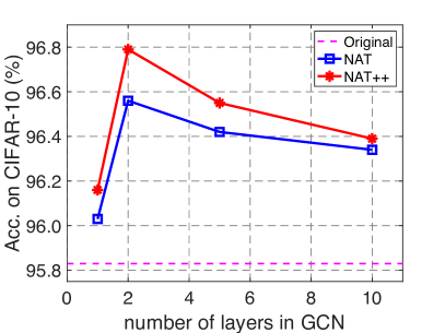
Note that a graph convolutional layer is able to extract features by aggregating the information from the neighbors of each node (i.e., one-hop neighbors) [47]. Nevertheless, building the model with too many graph convolutional layers (i.e., high-order model) may introduce redundant information [48] and hamper the performance (See results in Fig. 7(a)). In practice, we build our NAT with a two-layer GCN, which can be formulated as

$$\small{\bf{Z}}=f({\bf X},{\bf A})=h\left({\bf A}{\rm\sigma}\left({\bf A}{\bf X}{\bf W}^{(0)}\right){\bf W}^{(1)}{\bf W}^{\rm FC}\right),$$ (3)

where ${\bf W}^{(0)}$ and ${\bf W}^{(1)}$ denote the weights of two graph convolution layers, ${\bf W}^{\rm FC}$ denotes the weight of the fully-connected layer, $\sigma$ is a non-linear activation function (e.g., ReLU [49]), $h(\cdot)$ denotes the softmax layer, and ${\bf{Z}}$ refers to the probability distribution of $\pi(\cdot|\beta;\theta)$ over 3 transitions on the edges, i.e., “remaining unchanged”, “replacing with null connection”, and “replacing with skip connection”. It is worth mentioning that, the controller model is essentially a 3-class GCN based classifier. Given $K$ edges in an architecture, NAT outputs the probability distribution ${\bf{Z}}\in{\mathbb{R}}^{K\times 3}$. For convenience, we denote $\theta=\{{\bf W}^{(0)},{\bf W}^{(1)},{\bf W}^{\rm FC}\}$ as the parameters of the controller model of NAT.

Algorithm 1 Training method for NAT.

0:  The number of sampled input architectures in an iteration $m$, the number of sampled optimized architectures for each input architecture $n$, learning rate $\eta$, regularizer parameter $\lambda$ in Eqn. (4), input architecture distribution $p(\cdot)$.

1:  Initialize the parameters $\theta$ and $w$.

2:  while not convergent do

3:     for each iteration on training data do

4:        // Fix $\theta$ and update $w$.

5:        Sample $\beta_{i}\sim p(\cdot)$ to construct a batch $\{\beta_{i}\}_{i=1}^{m}$.

6:        Update supernet parameters $w$ by descending the gradient:

7:         

$$w\leftarrow w-\eta\frac{1}{m}\sum_{i=1}^{m}\nabla_{w}\mathcal{L}(\beta_{i},w).$$

8:     end for

9:     for each iteration on validation data do

10:        // Fix $w$ and update $\theta$.

11:        Sample $\beta_{i}\sim p(\cdot)$ to construct a batch $\{\beta_{i}\}_{i=1}^{m}$.

12:        Obtain $\{\alpha_{j}\}_{j=1}^{n}$ according to the policy learned by GCN.

13:        Update transformer parameters $\theta$ by ascending the gradient:

14:         

$$\theta\leftarrow \theta+\eta\frac{1}{mn}\sum_{i=1}^{m}\sum_{j=1}^{n}\Big{[}\nabla_{\theta}\log\pi(\alpha_{j}|\beta_{i};\theta)R(\alpha_{j}|\beta_{i})$$

$$+ \lambda\nabla_{\theta}H\big{(}\pi\left(\cdot|\beta_{i};\theta\right)\big{)}\Big{]}.$$

15:     end for

16:  end while

3.4 Training Method for NAT

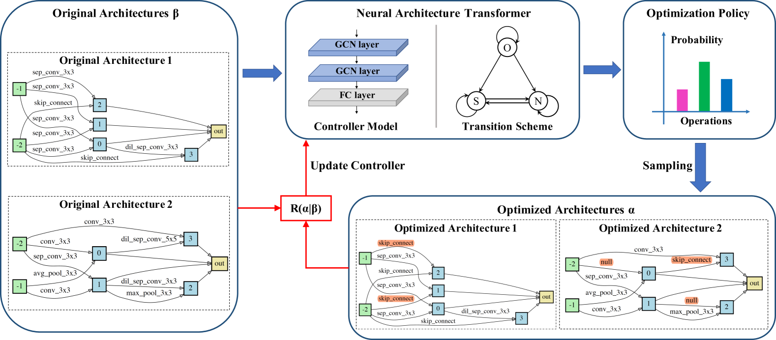
As shown in Fig. 3, given an architecture $\beta$ as input, NAT outputs the policy/distribution $\pi(\cdot|\beta;\theta)$ over different candidate transitions. Based on $\pi(\cdot|\beta;\theta)$, we conduct sampling to obtain the optimized architecture $\alpha$. After that, we compute the reward $R(\alpha|\beta)$ to guide the search process. To learn NAT, we first update the supernet parameters $w$ and then update the architecture transformer parameters $\theta$ in each iteration. We show the detailed training procedure in Algorithm 1.

Training the parameters of the supernet $w$. Given any $\theta$, we need to update the supernet parameters $w$ based on the training data. To accelerate the training process, we adopt the parameter sharing technique [17]. Then, we can use the shared parameters $w$ to represent the parameters for different architectures. For any architecture $\beta\sim p(\cdot)$, let $\mathcal{L}(\beta,w)$ be the loss function, e.g., the cross-entropy loss. Then, given any $m$ sampled architectures, the updating rule for $w$ with parameter sharing can be given by $w\leftarrow w-\eta\frac{1}{m}\sum_{i=1}^{m}\nabla_{w}\mathcal{L}(\beta_{i},w)$, where $\eta$ is the learning rate.

Training the parameters of the controller model $\theta$. We train the transformer with reinforcement learning (i.e., policy gradient) [50] for several reasons. First, from Eqn. (2), there are no supervision signals (i.e., “ground-truth” better architectures) to train the model in a supervised manner. Second, the metrics of both accuracy and computational cost are non-differentiable. As a result, the gradient-based methods cannot be directly used for training. To address these issues, we use reinforcement learning to train our model by maximizing the expected reward over the optimization results of different architectures.

To encourage exploration, we use an entropy regularization term in the objective to prevent the transformer from converging to a local optimum too quickly [51], e.g., selecting the “original” option for all the operations. The objective can be formulated as

$$J(\theta)=\mathbb{E}_{\beta\sim p(\cdot)}[\mathbb{E}_{\alpha\sim\pi(\cdot|\beta;\theta)}\left[{R}\left(\alpha|\beta\right)\right]{+}\lambda H\big{(}\pi(\cdot|\beta;\theta)\big{)}]$$ (4)

$$=\sum_{\beta}p(\beta)\big{[}\sum_{\alpha}\pi(\alpha|\beta;\theta)\big{(}{R}\left(\alpha|\beta\right)\big{)}+\lambda H\big{(}\pi(\cdot|{\beta};\theta)\big{)}\big{]},$$

where $p(\beta)$ is the probability to sample some architecture $\beta$ from the distribution $p(\cdot)$, $\pi(\alpha|\beta;\theta)$ is the probability to sample some architecture $\alpha$ from the distribution $\pi({\cdot|\beta};\theta)$, $H(\cdot)$ evaluates the entropy of the policy, and $\lambda$ controls the strength of the entropy regularization term. For each input architecture, we sample $n$ optimized architectures $\{\alpha_{j}\}_{j=1}^{n}$ from the distribution $\pi(\cdot|\beta;\theta)$ in each iteration. Thus, the gradient of Eqn. (4) w.r.t. $\theta$ becomes

$$\nabla_{\theta}J(\theta) \approx\frac{1}{mn}\sum_{i=1}^{m}\sum_{j=1}^{n}\Big{[}\nabla_{\theta}\log\pi(\alpha_{j}|\beta_{i};\theta)R(\alpha_{j}|\beta_{i})$$ (5)

$$+\lambda\nabla_{\theta}H\big{(}\pi(\cdot|\beta_{i};\theta)\big{)}\Big{]}.$$

The regularization term $H\big{(}\pi(\cdot|\beta_{i};\theta)\big{)}$ encourages the distribution $\pi(\cdot|\beta;\theta)$ to have high entropy, i.e., high diversity in the decisions on the edges. Thus, the decisions for some operations would be encouraged to choose the “skip” or “null” operations during training. In this sense, NAT is able to explore the whole search space to find the optimal architecture.

3.5 Inferring the Optimized Architectures

After the training process in Algorithm 1, we obtain the parameters $\theta$ of the architecture transformer model ${\rm NAT}(\cdot;\theta)$. Based on the NAT model, we take any given architecture $\beta$ as input and output the architecture optimization policy $\pi(\cdot|\beta;\theta)$. Then, we conduct sampling according to the learned policy to obtain the optimized architecture, i.e., $\alpha{\sim}\pi(\cdot|\beta;\theta)$. Specifically, we predict the optimal transition among three candidate transitions (i.e., “remaining unchanged”, “replacing with null connection”, and “replacing with skip connection”) for each edge in the architecture graph. Note that the sampling method is not an iterative process and we perform sampling once for each operation/edge. We can also obtain the optimized architecture by selecting the operation with the maximum probability, which, however, tends to reach a local optimum and yields worse results than the sampling based method (See results in supplementary).

Figure 4: Operation transition scheme of NAT++. (a) Two-level transition rule of NAT++; (b) Computational cost of different operations. We set the input channel and output channel to 128, the height and width of the input feature maps to 32. Here, sep denotes a separable convolution and dil denotes a dilated separable convolution.

4 Neural Architecture Transformer++

As mentioned in Section 3, NAT replaces the redundant operations in $O$ with the null connections $N$ or the skip connections $S$ according to the transition scheme in Fig. 2. However, there are still several limitations of NAT. First, merely replacing an operation with the null or skip connection makes the search space very small and may hamper the performance of architecture optimization. Second, when we divide $O$ into more specific operations, the number of transitions between every two categories would significantly increase. As a result, it is non-trivial to manually design valid transitions for each operation using NAT. Third, since operations may have different valid transitions to reduce the computational cost, it is hard to build a general GCN based classifier to predict the optimal transitions for all the operations.

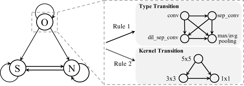
To address the above limitations, we further consider more possible operation transitions to enlarge the search space and develop more flexible operation transition rules. The proposed method is called Neural Architecture Transformer++ (NAT++), whose operation transition scheme is shown in Fig. 4. In NAT++, we propose a two-level transition rule which encourages operations to have more efficient types or smaller kernel sizes to produce more compact architectures. Note that different operations may have different valid transitions. To predict the optimal transitions for the operations with different valid transitions, we propose a Binary-Masked Softmax (BMSoftmax) layer to build the NAT++ model. We will depict our NAT++ in the following.

4.1 Operation Transition Scheme for NAT++

Note that NAT [21] only considers three operation transitions, i.e., remaining unchanged, replacing with null connection, replacing with skip connection. As a result, the search space may be very limited and may hamper the performance of architecture optimization. To consider a larger search space, we propose a two-level transition scheme which encourages operations to have more efficient types and/or smaller kernel sizes (See Fig. 4).

4.1.1 Two-level Transition Scheme

In NAT++, we consider a larger search space to enable more possible transitions for architecture optimization. Specifically, we allow the transitions among six operation types, namely standard convolution, separable convolution, dilated separable convolution, max/average pooling, skip connection, and null connection. For each operation type, we consider three kernel sizes, i.e., $1{\times}1$, $3{\times}3$, and $5{\times}5$. To optimize both the type and kernel size of operations, we design a type transition rule and a kernel transition rule, respectively.

• Type Transition: We seek to reduce the computational cost by changing operation into a more computationally efficient one. According to Fig. 4, we use the following rule:

  $$\text{{Rule 1:} conv}\rightarrow\text{sep\_conv}\rightarrow\text{dil\_sep\_conv}\rightarrow\text{pooling},$$

  where $\rightarrow$ denotes the transition direction. Since max pooling has a similar computational cost to average pooling, we enable the transition between max pooling and average pooling.

• Kernel Transition: Given a specific operation type, one can also adjust the kernel size to change the operation. In general, a larger kernel would induce higher computational cost. Thus, to make sure that all the transitions can reduce the computational cost, we consider the following rule:

  $$\text{Rule 2: }5\times 5\rightarrow 3\times 3\rightarrow 1\times 1.$$

It is worth noting that only using any of the two rules cannot guarantee that we can reduce the computational cost. Specifically, according to Fig. 4, if we only focus on the rule on operation type, there may still exist some transitions that increase the computational cost by changing the operation type to a more efficient one but increasing the kernel size, e.g., conv_$1{\times}1$ $\to$ sep_conv_$3{\times}3$. Similarly, if we only reduce the kernel size, there may also exist some transitions that introduce extra computational cost by changing the operation type to a more expensive one, e.g., sep_conv_$5{\times}5$ $\to$ conv_$3{\times}3$. Thus, in practice, we make all the transitions meet the above two rules simultaneously to avoid increasing the computational cost. With the proposed two-level transition rule, unlike NAT, our NAT++ is able to automatically obtain the valid transitions for all the operations.

4.1.2 Search Space of NAT++

NAT++ has more possible transitions than NAT and thus has a larger search space. Given a cell structure with $|{\mathcal{V}}|$ nodes and $2(|{\mathcal{V}}|{\small-}3)$ edges, we consider 13 operations/states in total (See more details in Fig. 4 and supplementary). Based on a specific $\beta$, the size of the largest search space of NAT++ is $|\Omega_{\beta}|=13^{2(|{\mathcal{V}}|-3)}$, which is larger than the largest search space of NAT with the size of $|\Omega_{\beta}|=3^{2(|{\mathcal{V}}|-3)}$. Therefore, NAT++ has the ability to find the architectures with better performance and lower computational cost than NAT (See results in Section 5). Note that NAT++ also allows the transitions $O{\to}S$, $O{\to}N$, and $S{\leftrightarrow}N$. Hence, the search space of NAT is a true subset of the search space of NAT++.

4.1.3 Complexity Analysis of Different Operations

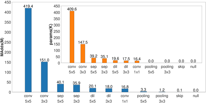
Note that our NAT and NAT++ seek to replace operations with the more efficient ones to avoid introducing additional computation cost. To determine which operations are more efficient, we compare the computational cost of different operations in terms of the number of multiply-adds (MAdds) and the number of parameters.

In Fig. 4, we sort the operations according to the number of parameters and MAdds in descending order. From Fig. 4, we draw the following observations. First, given a fixed kernel size, different operation types have different computational cost. Specifically, separable and dilated separable convolution have lower computational cost than the standard convolution. The max/average pooling, skip connection, and null connection have less or even no computational cost. Second, when we fix the operation type, the kernel size is also an important factor that affects the computational cost of operations. In general, a smaller kernel tends to have a lower computational cost.

4.2 Policy Learning for NAT++

To learn the optimal policy $\pi(\cdot|\beta;\theta)$ for NAT++, we also use a GCN based classifier to predict the optimal transition for each operation/edge. However, it is hard to directly apply the GCN based classifier in NAT to predict the optimal transitions for the operations with different valid transitions. Note that, in NAT, all the operations share the same valid transitions, i.e., remaining unchanged, replacing with null connection, replacing with skip connection. However, in NAT++, each operation has its own valid transitions and these transitions directly determine the considered classes of the GCN based classifier. As a result, we may have to design a GCN classifier for each operation, which, however, is very expensive in practice.

To address this issue, we make the following changes to build the GCN model of NAT++. First, we increase the number of output channels of the final FC layer to match all the considered operations. In this way, NAT++ is able to consider more possible transitions than NAT. Second, according to the transition scheme in Fig. 4, we replace the standard softmax layer in Eqn. (3) with a Binary-Masked Softmax (BMSoftmax) layer to omit all the invalid transitions that violate the two-level transition rule. Specifically, given $C$ different operations, we represent the transitions for each operation as a binary mask ${\bf v}\in{\mathbb{R}}^{C}$ (1 for valid transitions and 0 for invalid transitions). To omit the invalid transitions, NAT++ only computes the probabilities of all the valid transitions and leaves the probabilities of the invalid ones to be zero. Let ${\bf u}{\in}{\mathbb{R}}^{C}$ be the predicted logits by NAT++ over $C$ transitions. We compute the probability for the $i$-th transition by

$$h({\bf u},{\bf v})_{i}=\frac{{\bf v}_{i}\cdot e^{{\bf u}_{i}}}{\sum_{j=1}^{K}{\bf v}_{j}\cdot e^{{\bf u}_{j}}}.$$ (6)

Based on BMSoftmax, NAT++ is able to determine the optimal transition for the operations with different valid transitions.

4.3 Possible Bias Risk of NAT and NAT++

As shown in Figs. 2 and 4, both NAT and NAT++ seek to replace redundant operations with skip connections when optimizing architectures. However, the architectures with more skip connections tend to converge faster than other architectures [52, 53]. As a result, the competition between skip connections and other operations may easily become unfair [54] and mislead the search process. Consequently, the NAS methods may incur a bias towards those architectures which converge faster but may yield poor generalization performance [55, 52, 53]. More analysis on the bias issue can be found in supplementary.

To address the bias issue, Zhou et al.  introduce a binary gate to each operation and propose a path-depth-wise regularization method to encourage the gates along the long paths in the supernet [56]. Such a regularization forces NAS methods to explore the architectures with slow convergence speed. It is worth mentioning that, based on NAT and NAT++, we can alleviate the bias issue without the need for complex regularization. As shown in Algorithm 1, unlike ENAS [17] and DARTS [16], we decouple the supernet training from architecture search by sampling architectures from a uniform distribution $p(\cdot)$ rather than the learned policy $\pi(\cdot|\beta;\theta)$. Since all the operations have the same probability to be sampled, we provide an equal opportunity to train the architectures with different operations. In this sense, we can alleviate the possible bias issue (See results in Section 6.5). More critically, our methods are able to find better architectures than the architecture searched by [56] on ImageNet (See Table III).

TABLE I: Performance of the optimized architectures obtained by different methods based on hand-crafted architectures. “/” denotes the original models that are not changed by architecture optimization methods.

CIFAR						ImageNet
Model	Method	#Params (M)	#MAdds (M)	Acc. (%)		Model	Method	#Params (M)	#MAdds (M)	Acc. (%)
				CIFAR-10	CIFAR-100					Top-1	Top-5
VGG16	/	15.2	313	93.56	71.83	VGG16	/	138	15620	71.6	90.4
	NAO[20]	19.5	548	95.72	74.67		NAO [20]	148	18896	72.9	91.3
	ESNAC [40]	14.6	295	95.26	74.43		ESNAC [40]	133	14523	73.6	91.5
	APS [41]	15.0	305	95.53	74.79		APS [41]	137	15220	73.9	91.7
	NAT	15.2	315	96.04	75.02		NAT	138	15693	74.3	92.0
	NAT++	14.4	301	96.16	75.23		NAT++	131	14907	74.7	92.2
ResNet20	/	0.3	41	91.37	68.88	ResNet18	/	11.7	1580	69.8	89.1
	NAO [20]	0.4	61	92.44	71.22		NAO [20]	17.9	2246	70.8	89.7
	ESNAC [40]	0.3	40	92.87	71.58		ESNAC [40]	11.2	1544	71.0	89.9
	APS [41]	0.3	42	93.14	71.84		APS [41]	11.2	1547	70.9	90.0
	NAT	0.3	42	93.05	71.67		NAT	11.7	1588	71.1	90.0
	NAT++	0.3	39	93.23	71.97		NAT++	11.0	1516	71.3	90.2
ResNet56	/	0.9	127	93.21	71.54	ResNet50	/	25.6	3530	76.2	92.9
	NAO [20]	1.3	199	95.27	74.25		NAO [20]	34.8	4505	77.4	93.2
	ESNAC [40]	0.8	125	95.33	74.30		ESNAC [40]	25.0	3484	77.4	93.3
	APS [41]	0.8	123	94.54	73.58		APS [41]	24.9	3461	77.6	93.4
	NAT	0.9	129	95.40	74.33		NAT	25.6	3547	77.7	93.5
	NAT++	0.8	124	95.47	74.41		NAT++	24.8	3452	77.8	93.6
ShuffleNet	/	0.9	161	92.29	71.14	ShuffleNet	/	2.4	138	68.0	86.4
	NAO [20]	1.4	251	93.16	72.04		NAO [20]	3.5	217	68.2	86.5
	ESNAC [40]	0.8	153	93.21	72.14		ESNAC [40]	2.2	131	68.4	86.6
	APS [41]	0.9	161	93.47	72.40		APS [41]	2.4	138	68.9	87.0
	NAT	0.8	158	93.37	72.34		NAT	2.3	136	68.7	86.8
	NAT++	0.7	147	93.53	72.61		NAT++	2.1	125	68.8	87.0
MobileNetV2	/	2.3	91	94.47	73.66	MobileNetV2	/	3.4	300	72.0	90.3
	NAO [20]	2.9	131	94.75	73.79		NAO [20]	4.5	513	72.2	90.6
	ESNAC [40]	2.1	84	94.87	73.94		ESNAC [40]	3.1	277	72.4	90.8
	APS [41]	2.3	90	95.03	74.14		APS [41]	3.4	303	72.3	90.6
	NAT/NAT++	2.3	92	95.17	74.22		NAT/NAT++	3.4	302	72.5	91.0

TABLE II: Performance comparisons of the optimization results of hand-crafted architectures on face recognition datasets. “/” denotes the original models that are not changed by architecture optimization methods.

Model	Method	#Params (M)	#MAdds (M)	Acc. (%)
				LFW	CFP-FP	AgeDB-30
LResNet34E-IR [57]	/	31.8	7104	99.72	96.39	98.03
	NAO[20]	43.7	9874	99.73	96.41	98.07
	ESNAC [40]	31.7	7002	99.77	96.52	98.19
	APS [41]	31.6	6997	99.80	96.64	98.30
	NAT	31.8	7107	99.79	96.66	98.28
	NAT++	31.5	7023	99.83	96.72	98.35
MobileFaceNet [58]	/	1.0	441	99.50	92.23	95.63
	NAO [20]	1.3	584	99.53	92.28	95.75
	ESNAC [40]	0.9	408	99.59	92.37	95.98
	APS [41]	1.0	437	99.63	92.41	96.13
	NAT/NAT++	1.0	443	99.76	92.50	96.36

5 Experiments

We apply our method to optimize some well-designed architectures, including hand-crafted architectures and NAS based architectures. We have released the code for both NAT and NAT++ .

Figure 5: Architecture optimization results of several hand-crafted architectures. We provide both the views of graph (middle) and network (right).

5.1 Implementation Details

TABLE III: Comparisons of the optimized architectures obtained by different methods on NAS based architectures. “-” denotes that the results are not reported. “/” denotes the original models that are not changed by architecture optimization methods. ^† denotes the models trained with cutout.

CIFAR						ImageNet
Model	Method	#Params (M)	#MAdds (M)	Acc. (%)		Model	Method	#Params (M)	#MAdds (M)	Acc. (%)
				CIFAR-10	CIFAR-100					Top-1	Top-5
AmoebaNet† [59]	/	3.2	-	96.73	-	AmoebaNet [59]	/	5.1	555	74.5	92.0
PNAS† [60]		3.2	-	96.67	81.13	PNAS [60]		5.1	588	74.2	91.9
SNAS† [61]		2.9	-	97.08	82.47	SNAS [61]		4.3	522	72.7	90.8
GHN† [62]		5.7	-	97.22	-	GHN [62]		6.1	569	73.0	91.3
PR-DARTS† [56]		3.4	-	97.68	83.55	PR-DARTS [56]		5.0	543	75.9	92.7
ENAS† [17]	/	4.6	804	97.11	82.87	ENAS [17]	/	5.6	607	73.8	91.7
	NAO [20]	4.5	763	97.05	82.57		NAO [20]	5.5	589	73.7	91.7
	ESNAC [40]	4.1	717	97.13	83.15		ESNAC [40]	5.0	542	73.5	91.4
	APS [41]	4.4	744	97.26	83.45		APS [41]	5.5	591	74.0	91.9
	NAT	4.6	804	97.24	83.43		NAT	5.6	607	73.9	91.8
	NAT++	3.7	580	97.31	83.51		NAT++	5.4	582	74.3	92.1
DARTS† [16]	/	3.3	533	97.06	83.03	DARTS [16]	/	4.7	574	73.1	91.0
	NAO [20]	3.5	577	97.09	83.12		NAO [20]	5.0	621	73.3	91.1
	ESNAC [40]	2.8	457	97.21	83.36		ESNAC [40]	4.0	494	73.5	91.2
	APS [41]	3.2	515	97.25	83.44		APS [41]	4.5	539	73.3	91.2
	NAT	2.7	424	97.28	83.49		NAT	4.0	441	73.7	91.4
	NAT++	2.5	395	97.30	83.56		NAT++	3.8	413	73.9	91.5
NAONet† [20]	/	128	66016	97.89	84.33	NAONet [20]	/	11.3	1360	74.3	91.8
	NAO [20]	143	73705	97.91	84.42		NAO [20]	11.8	1417	74.5	92.0
	ESNAC [40]	107	55187	97.98	84.49		ESNAC [40]	9.5	1139	74.6	92.1
	APS [41]	125	63468	97.96	84.47		APS [41]	11.0	1286	74.5	92.1
	NAT	113	58326	98.01	84.53		NAT	8.4	1025	74.8	92.3
	NAT++	101	51976	98.07	84.60		NAT++	8.1	992	75.0	92.5
PC-DARTS† [63]	/	3.6	570	97.43	84.21	PC-DARTS [63]	/	5.3	597	75.8	92.7
	NAO [20]	4.7	725	97.49	84.30		NAO [20]	6.7	706	76.0	92.8
	ESNAC [40]	3.3	503	97.44	84.20		ESNAC [40]	4.7	529	75.9	92.7
	APS [41]	3.4	529	97.47	84.28		APS [41]	5.0	557	76.0	92.7
	NAT	3.4	518	97.51	84.31		NAT	4.9	546	76.1	92.8
	NAT++	3.3	512	97.57	84.37		NAT++	4.8	540	76.3	93.0

We build the supernet by stacking 8 cells with the initial channel number of 20. We train the transformer for 200 epochs. Following the setting of [16], we set $m=1$, $n=1$, and $\lambda=0.003$ in Eqn. (5). To cover all possible architectures, we set $q(\cdot)$ to be a uniform distribution. For the evaluation of networks, we replace the original cells with the optimized cells and train the models from scratch. For all the considered architectures, we follow the same settings of the original papers, i.e., we build the models with the same number of layers and channels as the original ones. We only apply cutout to the NAS based architectures on CIFAR.

5.2 Results on Hand-crafted Architectures

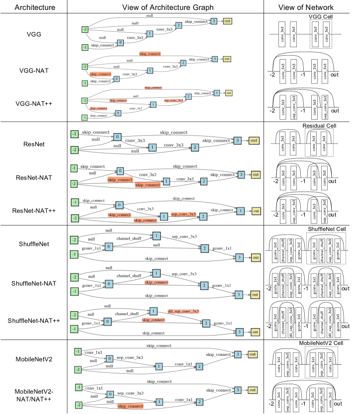
In this experiment, we apply both NAT and NAT++ to four popular hand-crafted architectures, namely VGG [14], ResNet [15], ShuffleNet [25] and MobileNetV2 [24]. To make all architectures share the same graph representation method defined in Section 3.2, we add null connections into the hand-crafted architectures to ensure that each node has two input nodes (See Fig. 5). Note that each hand-crafted architecture may have multiple graph representations. However, our methods yield stable results on different graph representations (See results in supplementary).

5.2.1 Quantitative Results

From Table I, our NAT based models consistently outperform the original models by a large margin with approximately the same computational cost. Compared to NAT, NAT++ produces better optimized architectures with higher accuracy and lower computational cost. These results show that, by enlarging the search space, NAT++ is able to further improve the performance of architecture optimization. Moreover, compared to existing methods (i.e., NAO, ESNAC and ASP), NAT++ produces the architectures with higher accuracy and lower computational cost. Note that NAT and NAT++ yield the same results when optimizing MobileNetV2. The main reason is that the operations in MobileNetV2 are either conv_$1{\times}1$ or sep_conv_$3{\times}3$, which have already been very efficient operations. Thus, it is hard to benefit from the extended transition scheme of NAT++ when there are very few valid operation transitions.

We also evaluate our method on face recognition tasks. In this experiment, we consider three benchmark datasets (i.e., LFW [64], CFP-FP [65] and AgeDB-30 [66]) and two baselines (i.e., LResNet34E-IR [57] and MobileFaceNet [58]). We adopt the same settings as that in [57]. More training details can be found in the supplementary. From Table II, the models optimized by NAT consistently outperform the original models without introducing extra computational cost. Moreover, NAT++ yields the best optimization results w.r.t. both architectures on all datasets.

5.2.2 Visualization of the Optimized Architectures

In this section, we visualize the original and optimized hand-crafted architectures in Fig. 5. From Fig. 5, NAT is able to introduce additional skip connections to the architecture to improve the architecture design. Unlike NAT, NAT++ conducts architecture optimization in a finer manner. Specifically, NAT++ replaces some standard convolutions with separable convolutions for VGG and ResNet. In this way, NAT++ not only reduces the number of parameters and computational cost but also further improves the performance (See Table I).

5.3 Results on NAS Based Architectures

We also apply the proposed methods to the automatically searched architectures. In this experiment, we consider four state-of-the-art NAS based architectures, namely DARTS [16], ENAS [17], NAONet [20] and PC-DARTS [63]. Moreover, we compare our optimized architectures with other NAS based architectures, including AmoebaNet [59], PNAS [60], SNAS [61], GHN [62], and PR-DARTS [56].

Figure 6: Effect of NAT and NAT++ on the average performance over 20 randomly sampled architectures on CIFAR-10.

From Table III, given different input architectures, the architectures obtained by NAT consistently yield higher accuracy than their original counterparts and the architectures optimized by existing methods. For example, given DARTS as input, NAT not only reduces 15% parameters and 23% computational cost but also achieves 0.6% improvement in terms of Top-1 accuracy on ImageNet. For NAONet, NAT reduces approximately 25% parameters and computational cost, and achieves 0.5% improvement in terms of Top-1 accuracy. Moreover, we also evaluate the architectures optimized by NAT++. As shown in Table III, equipped with the extended transition scheme, NAT++ is able to find better architectures with higher accuracy and lower computational cost than the architectures found by NAT and existing methods. Due to the page limit, we show the visualization results of the optimized architectures in the supplementary. These results show the effectiveness of the proposed method.

6 Further Experiments

(a) Number of layers vs. Accuracy.

(b) Value of $\lambda$ vs. Accuracy.

Figure 7: Effect of the number of layers in GCN and the value of $\lambda$ on the performance of NAT and NAT++.

(a) Convergence curves of Arch1.

(b) Convergence curves of Arch2.

(c) Convergence curves of Arch3.

(d) Convergence curves of Arch4.

Figure 8: Comparisons of convergence between the original architectures and the optimized architectures by NAT and NAT++ on CIFAR-10.

6.1 Results on Randomly Sampled Architectures

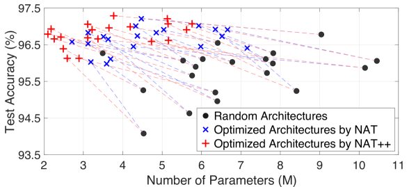
We apply our NAT and NAT++ to 20 randomly sampled architectures from the whole architecture space. We train all architectures using momentum SGD with a batch size of 128 for 600 epochs. From Table IV and Fig. 6, the architectures optimized by NAT surpass the original ones in terms of both accuracy and computational cost. Moreover, equipped with the two-level transition scheme, NAT++ further improves the architecture optimization results. To better illustrate this, we exhibit the result of each architecture in Fig. 6, which shows that the models optimized by NAT++ achieve higher accuracy with fewer parameters than NAT. In this sense, our method has good generalizability on a wide range of architectures, making it possible to be applied in real-world applications.

TABLE IV: Effect of NAT on the average performance over 20 randomly sampled architectures on CIFAR-10.

Method	Original	NAT	NAT++
#Params (M)	6.40$\pm$2.04	4.67$\pm$1.36	3.66$\pm$1.23
#MAdds (G)	1.07$\pm$0.32	0.79$\pm$0.21	0.52$\pm$0.20
Test accuracy (%)	95.83$\pm$1.08	96.56$\pm$0.47	96.79$\pm$0.32

6.2 Effect of the Number of Layers in GCN

We investigate the effect of the number of layers in GCN on the performance of our method. Specifically, we apply both NAT and NAT++ to optimize 20 randomly sampled architectures. We build 4 GCN models with $\{1,2,5,10\}$ layers, respectively. Note that a graph convolutional layer aims to extract features by aggregating the information from the neighbors of each node (i.e., one-hop neighbors) [47]. The GCN with multiple layers is able to exploit the information from multi-hop neighbors in a graph [67, 68].

From Fig. 7(a), when we build a single-layer GCN, the model yields very poor performance since a single-layer model cannot handle the information from the nodes with more than 1 hop. However, if we build the GCN model with 5 or 10 layers, the larger models also hamper the performance since the models with too many graph convolutional layers (i.e., high-order model) may introduce redundant information [48]. To learn a good policy, we build a two-layer GCN in practice.

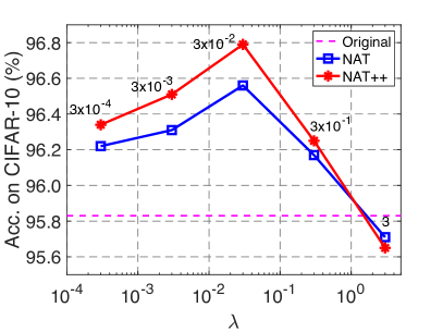
6.3 Effect of $\lambda$ in Eqn. (4)

In this part, we investigate the effect of $\lambda$ (which makes a trade-off between the reward and the entropy term in Eqn. (4)) on the performance of architecture optimization. We train NAT and NAT++ with $\lambda\in\{3{\times}10^{-4},3{\times}10^{-3},3{\times}10^{-2},3{\times}10^{-1},3\}$ and report the average accuracy over the optimization results of 20 randomly sampled architectures. From Fig. 7(b), when we increase $\lambda$ from $3{\times}10^{-4}$ to $3{\times}10^{-2}$, the entropy term gradually becomes more important and encourages the model to explore the search space. In this way, it prevents the model from converging to a local optimum and helps find better optimized architectures. If we further increase $\lambda$ to $3\times 10^{-1}$, the entropy term would overwhelm the objective function and hamper the performance. When we use a very large $\lambda=3$, the search process becomes approximately the same as random search and yields the architectures even worse than the original counterparts. In practice, we set $\lambda=3{\times}10^{-2}$.

TABLE V: Effect of $m$ and $n$ on the performance and search cost (GPU hour) of NAT and NAT++. We report the average performance on CIFAR-10 over the optimization results of 20 randomly sampled architectures.

m		1	5	10	30
NAT	Accuracy (%)	96.56$\pm$0.47	96.58$\pm$0.41	96.61$\pm$0.33	96.59$\pm$0.37
	Search Cost	5.3	19.9	38.9	122.7
NAT++	Accuracy (%)	96.79$\pm$0.32	96.80$\pm$0.37	96.83$\pm$0.29	96.81$\pm$0.34
	Search Cost	5.7	20.8	40.4	114.3
n		1	5	10	30
NAT	Accuracy (%)	96.56$\pm$0.47	96.59$\pm$0.41	96.57$\pm$0.43	96.58$\pm$0.39
	Search Cost	5.3	17.1	33.3	82.2
NAT++	Accuracy (%)	96.79$\pm$0.32	96.80$\pm$0.35	96.82$\pm$0.35	96.84$\pm$0.37
	Search Cost	5.7	18.2	35.1	86.7

6.4 Effect of $m$ and $n$ in Eqn. (5)

In this section, we investigate the effect of the hyper-parameters $m$ and $n$ on the performance of our method. When we gradually increase $m$ during training, more architectures have to be evaluated via additional forward propagations through the supernet to compute the reward. The search cost would significantly increase with the increase of $m$. From Table V, we do not observe obvious performance improvement when we consider a large $m$. One possible reason is that, based on the uniform distribution $p(\cdot)$, even sampling one architecture in each iteration has provided sufficient diversity of the input architectures to train our model. Thus, we set $m=1$ in practice.

We also investigate the effect of the hyper-parameter $n$ which controls the number of sampled optimized architectures for each input architecture. When we consider a large $n$, we have to evaluate more optimized architectures to compute the reward in each iteration, yielding significantly increased search cost. As shown in Table V, similar to $m$, our model only achieves marginal performance improvement with the increase of $n$. In practice, $n=1$ works well in NAT and NAT++. The main reason is that most of the sampled architectures can be very similar based on a fixed policy/distribution $\pi(\cdot|\beta;\theta)$. As a result, increasing the number of sampled optimized architectures may provide limited benefits for the training process. Actually, a similar phenomenon is also observed in ENAS [17].

6.5 Discussions on the Possible Bias Risk

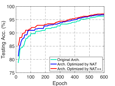
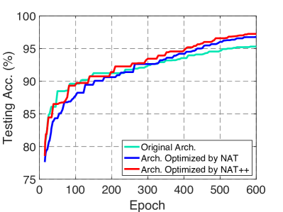
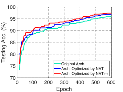
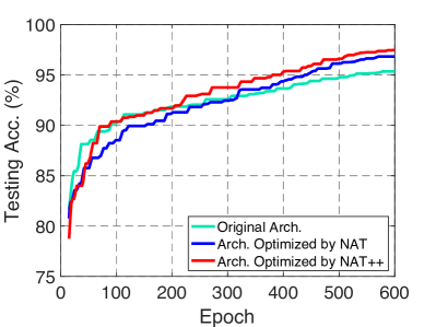
In this section, based on our methods, we investigate the possible bias issue towards the architectures that have fast convergence speed (in the early stage) but poor generalization performance. In this experiment, we randomly collect a set of architectures and use NAT and NAT++ to optimize them. Then, we compare the convergence curves of the original architectures and the optimized architectures on CIFAR-10. From Fig. 8, some of the original architectures incur the issue of “fast convergence in the early stage but with poor generalization performance”, e.g., Arch2 and Arch4. In contrast, all of the architectures optimized by NAT and NAT++ have a relatively stable convergence speed and yield better generalization performance than their original counterparts. From these results, the bias problem is not obvious in our methods. The main reason is that, in NAT and NAT++, all the operations have the same probability to be sampled and we would offer an equal opportunity to train the architectures with different operations. In this sense, we are able to alleviate the too fast convergence issue incurred by skip connection. Due to the page limit, we put the convergence curves of more architectures in the supplementary.

7 Conclusion

In this paper, we have proposed a novel Neural Architecture Transformer (NAT) for the task of architecture optimization. To solve this problem, we seek to replace the existing operations with more computationally efficient operations. Specifically, we propose a NAT to replace the redundant or non-significant operations with the skip connection or null connection. Moreover, we design an advanced NAT++ to further enlarge the search space. To be specific, we present a two-level transition rule which encourages operations to have a more efficient type or smaller kernel size to produce the more compact architectures. To verify the proposed method, we apply NAT and NAT++ to optimize both hand-crafted architectures and Neural Architecture Search (NAS) based architectures. Extensive experiments on several benchmark datasets demonstrate the effectiveness of the proposed method in improving the accuracy and compactness of neural architectures.

References

- [1] Y. LeCun, B. Boser, J. S. Denker, D. Henderson, R. E. Howard, W. Hubbard, and L. D. Jackel, “Backpropagation Applied to Handwritten zip Code Recognition,” Neural Computation, vol. 1, no. 4, pp. 541–551, 1989.
- [2] Y. Guo, Q. Wu, C. Deng, J. Chen, and M. Tan, “Double forward propagation for memorized batch normalization,” in AAAI Conference on Artificial Intelligence, 2018, pp. 3134–3141.
- [3] A. Krizhevsky, I. Sutskever, and G. E. Hinton, “Imagenet classification with deep convolutional neural networks,” in Advances in Neural Information Processing Systems, 2012, pp. 1097–1105.
- [4] R. K. Srivastava, K. Greff, and J. Schmidhuber, “Training Very Deep Networks,” in Advances in Neural Information Processing Systems, 2015, pp. 2377–2385.
- [5] Z. Jiang, Y. Zheng, H. Tan, B. Tang, and H. Zhou, “Variational deep embedding: An unsupervised and generative approach to clustering,” in International Joint Conference on Artificial Intelligence, 2017, pp. 1965–1972.
- [6] Y. Wei, W. Xia, M. Lin, J. Huang, B. Ni, J. Dong, Y. Zhao, and S. Yan, “Hcp: A flexible cnn framework for multi-label image classification,” IEEE Transactions on Pattern Analysis and Machine Intelligence, vol. 38, no. 9, pp. 1901–1907, 2015.
- [7] Y. Rao, J. Lu, J. Lin, and J. Zhou, “Runtime network routing for efficient image classification,” IEEE Transactions on Pattern Analysis and Machine Intelligence, 2018.
- [8] F. Schroff, D. Kalenichenko, and J. Philbin, “Facenet: A Unified Embedding for Face Recognition and Clustering,” in IEEE Conference on Computer Vision and Pattern Recognition, 2015, pp. 815–823.
- [9] Y. Sun, X. Wang, and X. Tang, “Deeply Learned Face Representations are Sparse, Selective, and Robust,” in IEEE Conference on Computer Vision and Pattern Recognition, 2015, pp. 2892–2900.
- [10] R. Ranjan, V. M. Patel, and R. Chellappa, “Hyperface: A deep multi-task learning framework for face detection, landmark localization, pose estimation, and gender recognition,” IEEE Transactions on Pattern Analysis and Machine Intelligence, vol. 41, no. 1, pp. 121–135, 2017.
- [11] S. Ren, K. He, R. Girshick, and J. Sun, “Faster r-cnn: Towards real-time object detection with region proposal networks,” IEEE Transactions on Pattern Analysis and Machine Intelligence, vol. 39, no. 6, pp. 1137–1149, 2016.
- [12] S. Ren, K. He, R. Girshick, X. Zhang, and J. Sun, “Object Detection Networks on Convolutional Feature Maps,” IEEE Transactions on Pattern Analysis and Machine Intelligence, 2016.
- [13] X. Zhang, J. Zou, K. He, and J. Sun, “Accelerating Very Deep Convolutional Networks for Classification and Detection,” IEEE Transactions on Pattern Analysis and Machine Intelligence, vol. 38, no. 10, pp. 1943–1955, 2016.
- [14] K. Simonyan and A. Zisserman, “Very deep convolutional networks for large-scale image recognition,” in International Conference on Learning Representations, 2015.
- [15] K. He, X. Zhang, S. Ren, and J. Sun, “Deep residual learning for image recognition,” in IEEE Conference on Computer Vision and Pattern Recognition, 2016, pp. 770–778.
- [16] H. Liu, K. Simonyan, and Y. Yang, “Darts: Differentiable architecture search,” in International Conference on Learning Representations, 2019.
- [17] H. Pham, M. Guan, B. Zoph, Q. Le, and J. Dean, “Efficient neural architecture search via parameter sharing,” in International Conference on Machine Learning, 2018, pp. 4095–4104.
- [18] B. Zoph and Q. V. Le, “Neural architecture search with reinforcement learning,” in International Conference on Learning Representations, 2017.
- [19] Y. Guo, Y. Chen, Y. Zheng, P. Zhao, J. Chen, J. Huang, and M. Tan, “Breaking the curse of space explosion: Towards efficient nas with curriculum search,” in International Conference on Machine Learning. PMLR, 2020, pp. 3822–3831.
- [20] R. Luo, F. Tian, T. Qin, E. Chen, and T.-Y. Liu, “Neural architecture optimization,” in Advances in Neural Information Processing Systems, 2018, pp. 7816–7827.
- [21] Y. Guo, Y. Zheng, M. Tan, Q. Chen, J. Chen, P. Zhao, and J. Huang, “Nat: Neural architecture transformer for accurate and compact architectures,” in Advances in Neural Information Processing Systems, 2019, pp. 735–747.
- [22] C. Szegedy, W. Liu, Y. Jia, P. Sermanet, S. Reed, D. Anguelov, D. Erhan, V. Vanhoucke, and A. Rabinovich, “Going deeper with convolutions,” in IEEE Conference on Computer Vision and Pattern Recognition, 2015, pp. 1–9.
- [23] A. G. Howard, M. Zhu, B. Chen, D. Kalenichenko, W. Wang, T. Weyand, M. Andreetto, and H. Adam, “Mobilenets: Efficient convolutional neural networks for mobile vision applications,” arXiv preprint arXiv:1704.04861, 2017.
- [24] M. Sandler, A. Howard, M. Zhu, A. Zhmoginov, and L.-C. Chen, “Mobilenetv2: Inverted residuals and linear bottlenecks,” in IEEE Conference on Computer Vision and Pattern Recognition, 2018, pp. 4510–4520.
- [25] X. Zhang, X. Zhou, M. Lin, and J. Sun, “Shufflenet: An extremely efficient convolutional neural network for mobile devices,” in IEEE Conference on Computer Vision and Pattern Recognition, 2018, pp. 6848–6856.
- [26] N. Ma, X. Zhang, H.-T. Zheng, and J. Sun, “Shufflenet v2: Practical guidelines for efficient cnn architecture design,” in European Conference on Computer Vision, 2018, pp. 116–131.
- [27] B. Baker, O. Gupta, N. Naik, and R. Raskar, “Designing neural network architectures using reinforcement learning,” in International Conference on Learning Representations, 2017.
- [28] Z. Zhong, J. Yan, W. Wu, J. Shao, and C.-L. Liu, “Practical block-wise neural network architecture generation,” in IEEE Conference on Computer Vision and Pattern Recognition, 2018, pp. 2423–2432.
- [29] H. Cai, L. Zhu, and S. Han, “ProxylessNAS: Direct neural architecture search on target task and hardware,” in International Conference on Learning Representations, 2019.
- [30] A. Vaswani, N. Shazeer, N. Parmar, J. Uszkoreit, L. Jones, A. N. Gomez, Ł. Kaiser, and I. Polosukhin, “Attention is all you need,” in Advances in Neural Information Processing Systems, 2017, pp. 5998–6008.
- [31] D. R. So, C. Liang, and Q. V. Le, “The evolved transformer,” in International Conference on Machine Learning, 2019.
- [32] T.-J. Yang, A. Howard, B. Chen, X. Zhang, A. Go, M. Sandler, V. Sze, and H. Adam, “Netadapt: Platform-aware neural network adaptation for mobile applications,” in European Conference on Computer Vision, 2018, pp. 285–300.
- [33] C. Lemaire, A. Achkar, and P.-M. Jodoin, “Structured pruning of neural networks with budget-aware regularization,” in IEEE Conference on Computer Vision and Pattern Recognition, 2019, pp. 9108–9116.
- [34] X. Dai, P. Zhang, B. Wu, H. Yin, F. Sun, Y. Wang, M. Dukhan, Y. Hu, Y. Wu, Y. Jia et al., “Chamnet: Towards efficient network design through platform-aware model adaptation,” in IEEE Conference on Computer Vision and Pattern Recognition, 2019, pp. 11 398–11 407.
- [35] T. Chen, I. Goodfellow, and J. Shlens, “Net2net: Accelerating learning via knowledge transfer,” in International Conference on Learning Representations, 2016.
- [36] H. Li, A. Kadav, I. Durdanovic, H. Samet, and H. P. Graf, “Pruning filters for efficient convnets,” in International Conference on Learning Representations, 2017.
- [37] Y. He, X. Zhang, and J. Sun, “Channel pruning for accelerating very deep neural networks,” in IEEE International Conference on Computer Vision, 2017, pp. 1398–1406.
- [38] J.-H. Luo, H. Zhang, H.-Y. Zhou, C.-W. Xie, J. Wu, and W. Lin, “Thinet: Pruning CNN filters for a thinner net,” in IEEE Transactions on Pattern Analysis and Machine Intelligence, vol. 41, no. 10, 2019, pp. 2525–2538.
- [39] Z. Zhuang, M. Tan, B. Zhuang, J. Liu, Y. Guo, Q. Wu, J. Huang, and J. Zhu, “Discrimination-aware channel pruning for deep neural networks,” in Advances in Neural Information Processing Systems, 2018, pp. 875–886.
- [40] S. Cao, X. Wang, and K. M. Kitani, “Learnable embedding space for efficient neural architecture compression,” in International Conference on Learning Representations, 2019.
- [41] J. Wang, H. Bai, J. Wu, X. Shi, J. Huang, I. King, M. Lyu, and J. Cheng, “Revisiting parameter sharing for automatic neural channel number search,” Advances in Neural Information Processing Systems, vol. 33, 2020.
- [42] K. He, X. Zhang, S. Ren, and J. Sun, “Identity mappings in deep residual networks,” in European Conference on Computer Vision, 2016, pp. 630–645.
- [43] J. Vermorel and M. Mohri, “Multi-armed bandit algorithms and empirical evaluation,” in European conference on machine learning. Springer, 2005, pp. 437–448.
- [44] V. Anantharam, P. Varaiya, and J. Walrand, “Asymptotically efficient allocation rules for the multiarmed bandit problem with multiple plays-part i: Iid rewards,” IEEE Transactions on Automatic Control, vol. 32, no. 11, pp. 968–976, 1987.
- [45] J. Schulman, S. Levine, P. Abbeel, M. Jordan, and P. Moritz, “Trust region policy optimization,” in International Conference on Machine Learning, 2015, pp. 1889–1897.
- [46] T. N. Kipf and M. Welling, “Semi-supervised classification with graph convolutional networks,” in International Conference on Learning Representations, 2016.
- [47] Z. Wu, S. Pan, F. Chen, G. Long, C. Zhang, and S. Y. Philip, “A comprehensive survey on graph neural networks,” IEEE Transactions on Neural Networks and Learning Systems, 2020.
- [48] Q. Zhu, B. Du, and P. Yan, “Multi-hop convolutions on weighted graphs,” arXiv preprint arXiv:1911.04978, 2019.
- [49] V. Nair and G. E. Hinton, “Rectified linear units improve restricted boltzmann machines,” in International Conference on Machine Learning, 2010, pp. 807–814.
- [50] R. J. Williams, “Simple statistical gradient-following algorithms for connectionist reinforcement learning,” Machine Learning, vol. 8, no. 3-4, pp. 229–256, 1992.
- [51] B. Zoph, V. Vasudevan, J. Shlens, and Q. V. Le, “Learning transferable architectures for scalable image recognition,” in IEEE Conference on Computer Vision and Pattern Recognition, 2018, pp. 8697–8710.
- [52] A. Zela, T. Elsken, T. Saikia, Y. Marrakchi, T. Brox, and F. Hutter, “Understanding and robustifying differentiable architecture search,” in International Conference on Learning Representations, 2019.
- [53] X. Chen and C.-J. Hsieh, “Stabilizing differentiable architecture search via perturbation-based regularization,” in International Conference on Machine Learning, 2020.
- [54] X. Chu, B. Zhang, R. Xu, and J. Li, “Fairnas: Rethinking evaluation fairness of weight sharing neural architecture search,” arXiv preprint arXiv:1907.01845, 2019.
- [55] Y. Shu, W. Wang, and S. Cai, “Understanding architectures learnt by cell-based neural architecture search,” in International Conference on Learning Representations, 2019.
- [56] P. Zhou, C. Xiong, R. Socher, and S. C. Hoi, “Theory-inspired path-regularized differential network architecture search,” in Advances in Neural Information Processing Systems, 2020.
- [57] J. Deng, J. Guo, N. Xue, and S. Zafeiriou, “Arcface: Additive angular margin loss for deep face recognition,” in Proceedings of the IEEE Conference on Computer Vision and Pattern Recognition, 2019, pp. 4690–4699.
- [58] S. Chen, Y. Liu, X. Gao, and Z. Han, “Mobilefacenets: Efficient cnns for accurate real-time face verification on mobile devices,” in Chinese Conference on Biometric Recognition. Springer, 2018, pp. 428–438.
- [59] E. Real, A. Aggarwal, Y. Huang, and Q. V. Le, “Regularized evolution for image classifier architecture search,” in AAAI Conference on Artificial Intelligence, vol. 33, 2019, pp. 4780–4789.
- [60] C. Liu, B. Zoph, M. Neumann, J. Shlens, W. Hua, L.-J. Li, L. Fei-Fei, A. Yuille, J. Huang, and K. Murphy, “Progressive neural architecture search,” in European Conference on Computer Vision, 2018, pp. 19–34.
- [61] S. Xie, H. Zheng, C. Liu, and L. Lin, “SNAS: Stochastic neural architecture search,” in International Conference on Learning Representations, 2019.
- [62] C. Zhang, M. Ren, and R. Urtasun, “Graph hypernetworks for neural architecture search,” in International Conference on Learning Representations, 2019.
- [63] Y. Xu, L. Xie, X. Zhang, X. Chen, G.-J. Qi, Q. Tian, and H. Xiong, “Pc-darts: Partial channel connections for memory-efficient differentiable architecture search,” in International Conference on Learning Representations, 2020.
- [64] G. B. Huang, M. Ramesh, T. Berg, and E. Learned-Miller, “Labeled faces in the wild: A database for studying face recognition in unconstrained environments,” Technical Report 07-49, University of Massachusetts, Amherst, Tech. Rep., 2007.
- [65] S. Sengupta, J.-C. Chen, C. Castillo, V. M. Patel, R. Chellappa, and D. W. Jacobs, “Frontal to profile face verification in the wild.” IEEE, 2016, pp. 1–9.
- [66] S. Moschoglou, A. Papaioannou, C. Sagonas, J. Deng, I. Kotsia, and S. Zafeiriou, “Agedb: the first manually collected, in-the-wild age database,” 2017, pp. 51–59.
- [67] X. V. Lin, R. Socher, and C. Xiong, “Multi-hop knowledge graph reasoning with reward shaping,” in Proceedings of the 2018 Conference on Empirical Methods in Natural Language Processing, EMNLP 2018, Brussels, Belgium, October 31-November 4, 2018, 2018.
- [68] M. Ding, C. Zhou, Q. Chen, H. Yang, and J. Tang, “Cognitive graph for multi-hop reading comprehension at scale,” in Proceedings of the 58th Annual Meeting of the Association for Computational Linguistics, 2019.