Concealed Object Detection

Abstract

We present the first systematic study on concealed object detection (COD), which aims to identify objects that are visually embedded in their background. The high intrinsic similarities between the concealed objects and their background make COD far more challenging than traditional object detection/segmentation. To better understand this task, we collect a large-scale dataset, called COD10K, which consists of 10,000 images covering concealed objects in diverse real-world scenarios from 78 object categories. Further, we provide rich annotations including object categories, object boundaries, challenging attributes, object-level labels, and instance-level annotations. Our COD10K is the largest COD dataset to date, with the richest annotations, which enables comprehensive concealed object understanding and can even be used to help progress several other vision tasks, such as detection, segmentation, classification etc. Motivated by how animals hunt in the wild, we also design a simple but strong baseline for COD, termed the Search Identification Network (SINet). Without any bells and whistles, SINet outperforms twelve cutting-edge baselines on all datasets tested, making them robust, general architectures that could serve as catalysts for future research in COD. Finally, we provide some interesting findings, and highlight several potential applications and future directions. To spark research in this new field, our code, dataset, and online demo are available at our project page: http://mmcheng.net/cod.

1 Introduction

Can you find the concealed object(s) in each image of Fig. 1 within 10 seconds? Biologists refer to this as background matching camouflage (BMC) [2], where one or more objects attempt to adapt their coloring to match “seamlessly” with the surroundings in order to avoid detection [3]. Sensory ecologists [4] have found that this BMC strategy works by deceiving the visual perceptual system of the observer. Naturally, addressing concealed object detection (COD) requires a significant amount of visual perception [6] knowledge. Understanding COD has not only scientific value in itself, but it also important for applications in many fundamental fields, such as computer vision (e.g., for search-and-rescue work, or rare species discovery), medicine (e.g., polyp segmentation [7], lung infection segmentation [8]), agriculture (e.g., locust detection to prevent invasion), and art (e.g., recreational art [9]).

In Fig. 2, we present examples of generic, salient, and concealed object detection. The high intrinsic similarities between the targets and non-targets make COD far more challenging than traditional object segmentation/detection [10, 11, 12]. Although it has gained increased attention recently, studies on COD still remain scarce, mainly due to the lack of a sufficiently large dataset and a standard benchmark like Pascal-VOC [13], ImageNet [14], MS-COCO [15], ADE20K [16], and DAVIS [17].

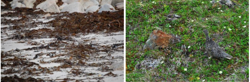
Figure 1: Examples of background matching camouflage (BMC). There are seven and six birds for the left and right image, respectively. Answers in color are shown in Fig. 27.

\begin{overpic}[width=433.62pt]{DifferentTask} \put(5.8,-3.5){\footnotesize(a) Image} \put(25.0,-3.5){\footnotesize(b) Generic object} \put(51.0,-3.5){\footnotesize(c) Salient object} \put(73.5,-3.5){\footnotesize(d) Concealed object} \end{overpic}

Figure 2: Task relationship. Given an input image (a), we present the ground-truth for (b) panoptic segmentation [5] (which detects generic objects [18, 19] including stuff and things), (c) instance level salient object detection [20, 11], and (d) the proposed concealed object detection task, where the goal is to detect objects that have a similar pattern to the natural environment. In this example, the boundaries of the two butterflies are blended with the bananas, making them difficult to identify.

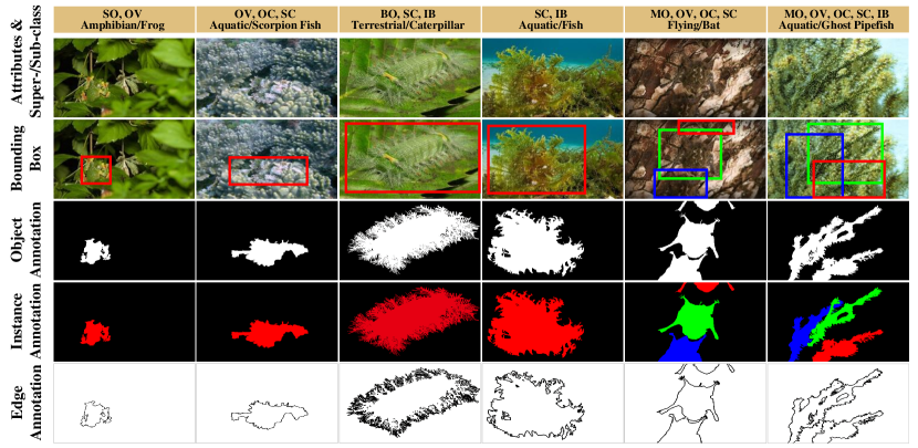
Figure 3: Annotation diversity in the proposed COD10K dataset. Instead of only providing coarse-grained object-level annotations like in previous works, we offer six different annotations for each image, which include attributes and categories ($1^{st}$ row), bounding boxes ($2^{nd}$ row), object annotation ($3^{rd}$ row), instance annotation ($4^{th}$ row), and edge annotation ($5^{th}$ row).

In this paper, we present the first complete study for the concealed object detection task using deep learning, bringing a novel view to object detection from a concealed perspective.

1.1 Contributions

Our main contributions are as follows:

• COD10K Dataset. With the goal mentioned above, we carefully assemble COD10K, a large-scale concealed object detection dataset. Our dataset contains 10,000 images covering 78 object categories, such as terrestrial, amphibians, flying, aquatic, etc. All the concealed images are hierarchically annotated with category, bounding-box, object-level, and instance-level labels (Fig. 3), benefiting many related tasks, such as object proposal, localization, semantic edge detection, transfer learning [21], domain adaption [22], etc. Each concealed image is assigned challenging attributes (e.g., shape complexity-SC, indefinable boundaries-IB, occlusions-OC) found in the real-world and matting-level [23] labeling (which takes $\sim$60 minutes per image). These high-quality labels could help provide deeper insight into the performance of models.

• COD Framework. We propose a simple but efficient framework, named SINet (Search Identification Net). Remarkably, the overall training time of SINet takes 4 hours and it achieves the new state-of-the-art (SOTA) on all existing COD datasets, suggesting that it could offer a potential solution to concealed object detection. Our network also yield several interesting findings (e.g., search and identification strategy is suitable for COD), making various potential applications more feasible.

• COD Benchmark. Based on the collected COD10K and previous datasets [24, 25], we offer a rigorous evaluation of 12 SOTA baselines, making ours the largest COD study. We report baselines in two scenarios, i.e., super-class and sub-class. We also track the community’s progress via an online benchmark (http://dpfan.net/camouflage/).

• Downstream Applications. To further support research in the field, we develop an online demo (http://mc.nankai.edu.cn/cod) to enable other researchers to test their scenes easily. In addition, we also demonstrate several potential applications such as medicine, manufacturing, agriculture, art, etc.

• Future Directions. Based on the proposed COD10K, we also discuss ten promising directions for future research. We find that concealed object detection is still far from being solved, leaving large room for improvement.

This paper is based on and extends our conference version [1] in terms of several aspects. First, we provide a more detailed analysis of our COD10K, including the taxonomy, statistics, annotations, and resolutions. Secondly, we improve the performance our SINet model by introducing neighbor connection decoder (NCD) and group-reversal attention (GRA). Thirdly, we conduct extensive experiments to validate the effectiveness of our model, and provide several ablation studies for the different modules within our framework. Fourth, we provide an exhaustive super-class and sub-class benchmarking and a more insightful discussion regarding the novel COD task. Last but not least, based on our benchmark results, we draw several important conclusions and highlight several promising future directions, such as concealed object ranking, concealed object proposal, concealed instance segmentation.

2 Related Work

In this section, we briefly review closely related works. Following [10], we roughly divide object detection into three categories: generic, salient, and concealed object detection.

TABLE I: Summary of COD datasets, showing that COD10K offers much richer annotations and benefits many tasks. Att.: Attribute label. BBox.: Bounding box label. Ml.: Alpha matting-level annotation [23]. Ins.: Instance-level label. Cate.: Category label. Obj.: Object-level label. Loc.: Location. Det.: Detection. Cls.: Classification. WS.: Weak Supervision. InSeg. Instance Segmentation.

	Statistics			Annotations						Data Split		Tasks
Dataset	Year	#Img.	#Cls.	Att.	BBox.	Ml.	Ins.	Cate.	Obj.	#Training	#Testing	Loc.	Det.	Cls.	WS.	InSeg.
CHAMELEON [24]	2018	76	N/A	$\times$	$\times$	$\times$	$\times$	$\times$	✓	0	76	✓	✓	$\times$	$\times$	$\times$
CAMO-COCO [25]	2019	2,500	8	✓	$\times$	$\times$	$\times$	$\times$	✓	1,250	1,250	✓	✓	$\times$	$\times$	$\times$
COD10K (OUR)	2020	10,000	78	✓	✓	✓	✓	✓	✓	6,000	4,000	✓	✓	✓	✓	✓

Generic Object Segmentation (GOS).   One of the most popular directions in computer vision is generic object segmentation [26, 27, 28, 5]. Note that generic objects can be either salient or concealed. Concealed objects can be seen as difficult cases of generic objects. Typical GOS tasks include semantic segmentation and panoptic segmentation (see Fig. 2 b).

Salient Object Detection (SOD).   This task aims to identify the most attention-grabbing objects in an image and then segment their pixel-level silhouettes [29, 30, 31]. The flagship products that make use of SOD technology [32] are Huawei’s smartphones, which employ SOD [32] to create what they call “AI Selfies”. Recently, Qin et al.  applied the SOD algorithm [33] to two (near) commercial applications: AR COPY & PASTE and OBJECT CUT. These applications have already drawn great attention (12K github stars) and have important real-world impacts.

Although the term “salient” is essentially the opposite of “concealed” (standout vs. immersion), salient objects can nevertheless provide important information for COD, e.g., images containing salient objects can be used as the negative samples. Giving a complete review on SOD is beyond the scope of this work. We refer readers to recent survey and benchmark papers [11, 34, 35, 36] for more details. Our online benchmark is publicly available at: http://dpfan.net/socbenchmark/.

Concealed Object Detection (COD).   Research into COD, which has had a tremendous impact on advancing our knowledge of visual perception, has a long and rich history in biology and art. Two remarkable studies on concealed animals from Abbott Thayer [37] and Hugh Cott [38] are still hugely influential. The reader can refer to the survey by Stevens et al.  [4] for more details on this history. There are also some concurrent works [39, 40, 41] that are accepted after this submission.

COD Datasets. CHAMELEON [24] is an unpublished dataset that has only 76 images with manually annotated object-level ground-truths (GTs). The images were collected from the Internet via the Google search engine using “concealed animal” as a keyword. Another contemporary dataset is CAMO [25], which has 2.5K images (2K for training, 0.5K for testing) covering eight categories. It has two sub-datasets, CAMO and MS-COCO, each of which contains 1.25K images. Unlike existing datasets, the goal of our COD10K is to provide a more challenging, higher quality, and more densely annotated dataset. COD10K is the largest concealed object detection dataset so far, containing 10K images (6K for training, 4K for testing). See Table I for details.

Types of Camouflage. Concealed images can be roughly split into two types: those containing natural camouflage and those with artificial camouflage. Natural camouflage is used by animals (e.g., insects, sea horses, and cephalopods) as a survival skill to avoid recognition by predators. In contrast, artificial camouflage is usually used in art design/gaming to hide information, occurs in products during the manufacturing process (so-called surface defects [42], defect detection [43, 44]), or appears in our daily life (e.g., transparent objects [45, 46, 47]).

COD Formulation. Unlike class-aware tasks such as semantic segmentation, concealed object detection is a class-agnostic task. Thus, the formulation of COD is simple and easy to define. Given an image, the task requires a concealed object detection algorithm to assign each pixel $i$ a label $Label_{i}\in$ {0,1}, where $Label_{i}$ denotes the binary value of pixel $i$. A label of 0 is given to pixels that do not belong to the concealed objects, while a label of 1 indicates that a pixel is fully assigned to the concealed objects. We focus on object-level concealed object detection, leaving concealed instance detection to our future work.

\begin{overpic}[width=433.62pt]{sub-classExample} \put(1.0,-1.0){sea-horse} \put(22.0,-1.0){cat} \put(40.0,-1.0){dog} \put(60.0,-1.0){bird} \put(72.0,-1.0){sea-lion} \put(87.0,-1.0){butterfly} \end{overpic}

Figure 4: Examples of sub-classes. Please refer to supplementary materials for other sub-classes.

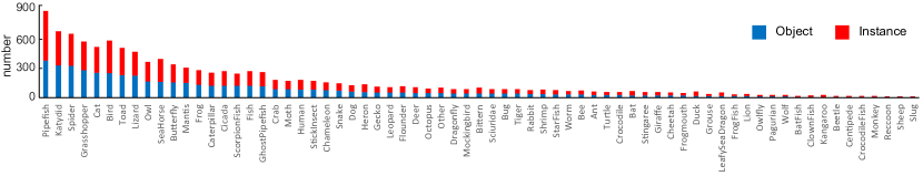
Figure 5: Object and instance distributions of each concealed category in the COD10K. COD10K consists of 5,066 concealed images from 69 categories. Zoom in for best view.

3 COD10K Dataset

The emergence of new tasks and datasets [48, 16, 49] has led to rapid progress in various areas of computer vision. For instance, ImageNet [50] revolutionized the use of deep models for visual recognition. With this in mind, our goals for studying and developing a dataset for COD are: (1) to provide a new challenging object detection task from the concealed perspective, (2) to promote research in several new topics, and (3) to spark novel ideas. Examples from COD10K are shown in Fig. 1. We will provide the details on COD10K in terms of three key aspects including image collection, professional annotation, and dataset features and statistics.

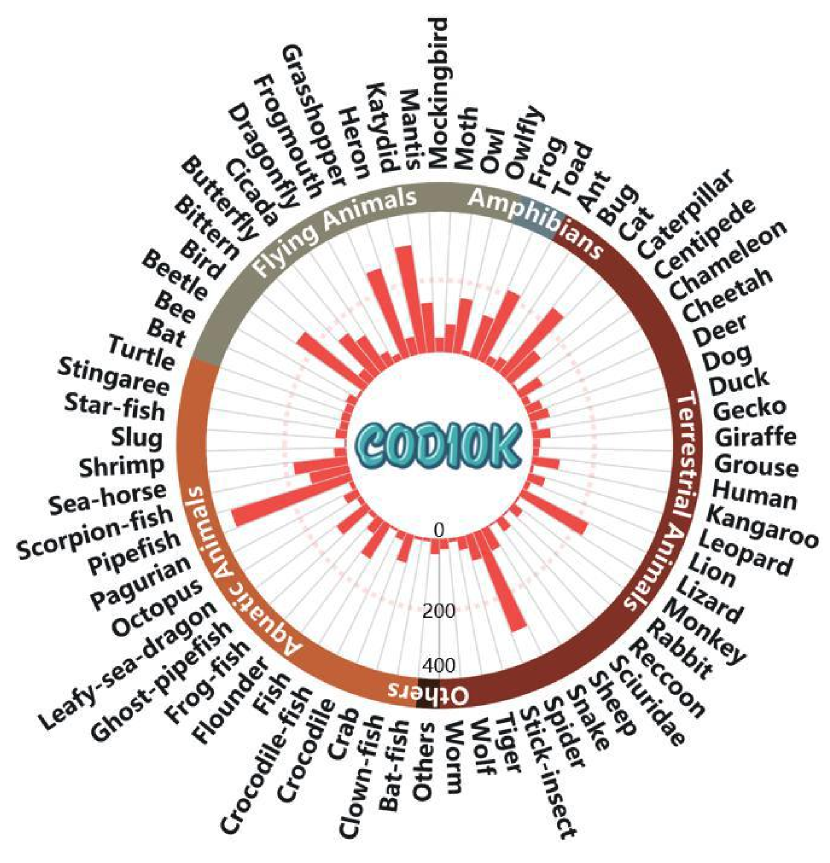
Figure 6: Taxonomic system. We illustrate the histogram distribution for the 69 concealed categories in our COD10K.

3.1 Image Collection

As discussed in [17, 51, 11], the quality of annotation and size of a dataset are determining factors for its lifespan as a benchmark. To this end, COD10K contains 10,000 images (5,066 concealed, 3,000 background, 1,934 non-concealed), divided into 10 super-classes (i.e., flying, aquatic, terrestrial, amphibians, other, sky, vegetation, indoor, ocean, and sand), and 78 sub-classes (69 concealed, 9 non-concealed) which were collected from multiple photography websites.

Most concealed images are from Flickr and have been applied for academic use with the following keywords: concealed animal, unnoticeable animal, concealed fish, concealed butterfly, hidden wolf spider, walking stick, dead-leaf mantis, bird, sea horse, cat, pygmy seahorses, etc. (see Fig. 4) The remaining concealed images (around 200 images) come from other websites, including Visual Hunt, Pixabay, Unsplash, Free-images, etc., which release public-domain stock photos, free from copyright and loyalties. To avoid selection bias [11], we also collected 3,000 salient images from Flickr. To further enrich the negative samples, 1,934 non-concealed images, including forest, snow, grassland, sky, seawater and other categories of background scenes, were selected from the Internet. For more details on the image selection scheme, we refer to Zhou et al.  [52].

3.2 Professional Annotation

Recently released datasets [51, 53, 54] have shown that establishing a taxonomic system is crucial when creating a large-scale dataset. Motivated by [55], our annotations (obtained via crowdsourcing) are hierarchical (category $\rightarrowtail$ bounding box $\rightarrowtail$ attribute $\rightarrowtail$ object/instance).

$\bullet$ Categories. As illustrated in Fig. 6, we first create five super-class categories. Then, we summarize the 69 most frequently appearing sub-class categories according to our collected data. Finally, we label the sub-class and super-class of each image. If the candidate image does not belong to any established category, we classify it as ‘other’.

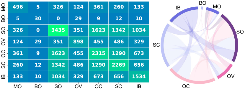
Attr.	Description
MO	Multiple Objects. Image contains at least two objects.
BO	Big Object. Ratio ($\tau_{bo}$) between object area and image area $\geq$0.5.
SO	Small Object. Ratio ($\tau_{so}$) between object area and image area $\leq$0.1.
OV	Out-of-View. Object is clipped by image boundaries.
OC	Occlusions. Object is partially occluded.
SC	Shape Complexity. Object contains thin parts (e.g., animal foot).
IB	Indefinable Boundaries. The foreground and background areas
	around the object have similar colors ($\chi^{2}$ distance $\tau_{gc}$ between
	RGB histograms less than 0.9).

Figure 7: Attribute distribution. Top-left: Co-attributes distribution over COD10K. The number in each grid indicates the total number of images. Top-right: Multi-dependencies among these attributes. A larger arc length indicates a higher probability of one attribute correlating to another. Bottom: attribute descriptions. Examples could be found in the first row of Fig. 3.

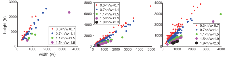
Figure 8: Image resolution (unit for the axis: pixel) distribution of COD datasets. From left to right: CHAMELEON [24], CAMO-COCO [25] and COD10K datasets.

$\bullet$ Bounding boxes. To extend COD10K for the concealed object proposal task, we also carefully annotate the bounding boxes for each image.

$\bullet$ Attributes. In line with the literature [11, 17], we label each concealed image with highly challenging attributes faced in natural scenes, e.g., occlusions, indefinable boundaries. Attribute descriptions and the co-attribute distribution is shown in Fig. 7.

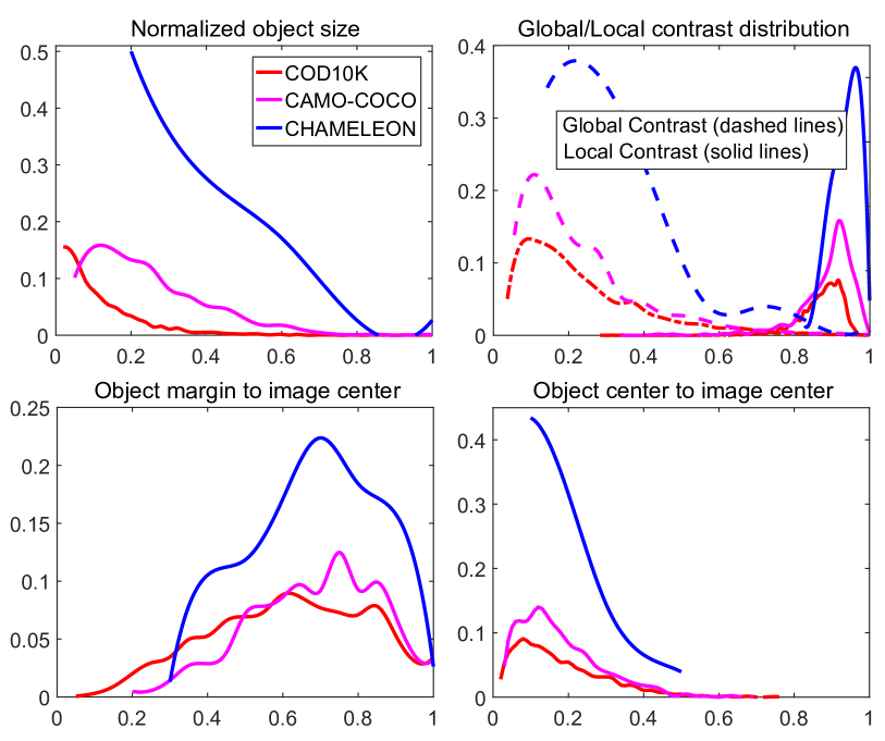
Figure 9: Comparison between the proposed COD10K and existing datasets. COD10K has smaller objects (top-left), contains more difficult conceale (top-right), and suffers from less center bias (bottom-left/right).

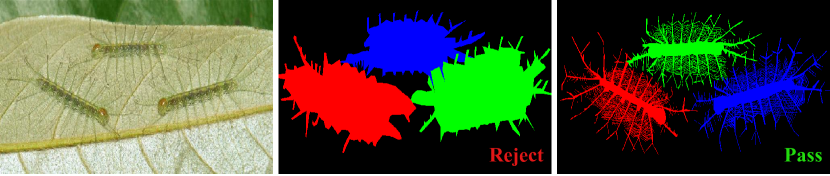
Figure 10: High-quality annotation. The annotation quality is close to the existing matting-level [23] annotation.

$\bullet$ Objects/Instances. We stress that existing COD datasets focus exclusively on object-level annotations (Table I). However, being able to parse an object into its instances is important for computer vision researchers to be able to edit and understand a scene. To this end, we further annotate objects at an instance-level, like COCO [15], resulting in 5,069 objects and 5,930 instances.

3.3 Dataset Features and Statistics

We now discuss the proposed dataset and provide some statistics.

$\bullet$ Resolution distribution. As noted in [56], high-resolution data provides more object boundary details for model training and yields better performance when testing. Fig. 8 presents the resolution distribution of COD10K, which includes a large number of Full HD 1080p resolution images.

$\bullet$ Object size. Following [11], we plot the normalized (i.e., related to image areas) object size in Fig. 9 (top-left), i.e., the size distribution from 0.01%$\sim$ 80.74% (avg.: 8.94%), showing a broader range compared to CAMO-COCO, and CHAMELEON.

$\bullet$ Global/Local contrast. To evaluate whether an object is easy to detect, we describe it using the global/local contrast strategy [57]. Fig. 9 (top-right) shows that objects in COD10K are more challenging than those in other datasets.

$\bullet$ Center bias. This commonly occurs when taking a photo, as humans are naturally inclined to focus on the center of a scene. We adopt the strategy described in [11] to analyze this bias. Fig. 9 (bottom-left/right) shows that our COD10K dataset suffers from less center bias than others.

$\bullet$ Quality control. To ensure high-quality annotation, we invited three viewers to participate in the labeling process for 10-fold cross-validation. Fig. 10 shows examples that were passed/rejected. This matting-level annotation costs $\sim$ 60 minutes per image on average.

$\bullet$ Super/Sub-class distribution. COD10K includes five concealed super-classes (i.e., terrestrial, atmobios, aquatic, amphibian, other) and 69 sub-classes (e.g., bat-fish, lion, bat, frog, etc). Examples of the word cloud and object/instance number for various categories are shown in Fig. 5 & Fig. 11, respectively.

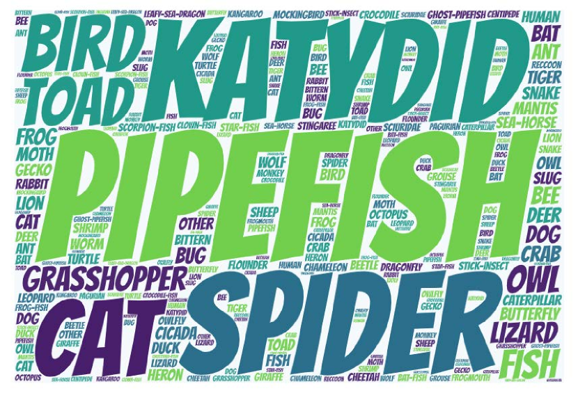
Figure 11: Word cloud distribution. The size of a specific word is proportional to the ratio of that keyword.

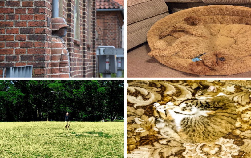
Figure 12: Diverse types of concealed objects in our COD10K. For instance, concealed human in art ($1^{st}$ column), and concealed animals ($2^{nd}$ column) in our daily life.

$\bullet$ Dataset splits. To provide a large amount of training data for deep learning algorithms, our COD10K is split into 6,000 images for training and 4,000 for testing, randomly selected from each sub-class.

$\bullet$ Diverse concealed objects. In addition to the general concealed patterns, such as those in Fig. 1, our dataset also includes various other types of concealed objects, such as concealed body paintings and conceale in daily life (see Fig. 12).

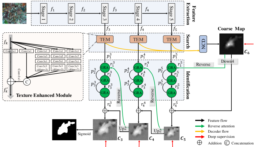
Figure 13: Pipeline of our SINet framework. It consists of three main components: the texture enhanced module (TEM), neighbor connection decoder (NCD), and group-reversal attention (GRA). The TEM is introduced to mimic the textural structure of receptive fields in the human visual system. The NCD is responsible for locating the candidates with the assistance of the TEM. The GRA blocks reproduce the identification stages of animal predation. Note that $f^{\prime}_{k}$ = $p_{1}^{k}$.

4 COD Framework

4.1 Network Overview

Fig. 13 illustrates the overall concealed object detection framework of the proposed SINet (Search Identification Network). Next, we explain our motivation and introduce the network overview.

Motivation.   Biological studies [58] have shown that, when hunting, a predator will first judge whether a potential prey exists, i.e., it will search for a prey. Then, the target animal can be identified; and, finally, it can be caught.

Introduction.   Several methods [59, 60] have shown that satisfactory performance is dependent on the re-optimization strategy (i.e., coarse-to-fine), which is regarded as the composition of multiple sub-steps. This also suggests that decoupling the complicated targets can break the performance bottleneck. Our SINet model consists of the first two stages of hunting, i.e., search and identification. Specifically, the former phase (Section 4.2) is responsible for searching for a concealed object, while the latter one (Section 4.3) is then used to precisely detect the concealed object in a cascaded manner.

Next, we elaborate on the details of the three main modules, including a) the texture enhanced module (TEM), which is used to capture fine-grained textures with the enlarged context cues; b) the neighbor connection decoder (NCD), which is able to provide the location information; and c) the cascaded group-reversal attention (GRA) blocks, which work collaboratively to refine the coarse prediction from the deeper layer.

4.2 Search Phase

Feature Extraction.   For an input image $\mathbf{I}\!\in\!\mathbb{R}^{W\!\times\!H\!\times\!3}$, a set of features $f_{k},k\in\{1,2,3,4,5\}$ is extracted from Res2Net-50 [61] (removing the top three layers, i.e., ‘average pool’, ‘1000-d fc’, and ‘softmax’). Thus, the resolution of each feature $f_{k}$ is ${H/2^{k}\times W/2^{k}},k\in\{1,2,3,4,5\}$, covering diversified feature pyramids from high-resolution, weakly semantic to low-resolution, strongly semantic.

Texture Enhanced Module (TEM).   Neuroscience experiments have verified that, in the human visual system, a set of various sized population receptive fields helps to highlight the area close to the retinal fovea, which is sensitive to small spatial shifts [62]. This motivates us to use the TEM [63] to incorporate more discriminative feature representations during the searching stage (usually in a small/local space). As shown in Fig. 13, each TEM component includes four parallel residual branches $\{b_{i},i=1,2,3,4\}$ with different dilation rates $d\in\{1,3,5,7\}$ and a shortcut branch (gray arrow), respectively. In each branch $b_{i}$, the first convolutional layer utilizes a $1\times 1$ convolution operation (Conv1$\times$1) to reduce the channel size to 32. This is followed by two other layers: a $(2i-1)\times(2i-1)$ convolutional layer and a $3\times 3$ convolutional layer with a specific dilation rate $(2i-1)$ when $i>1$. Then, the first four branches $\{b_{i},i=1,2,3,4\}$ are concatenated and the channel size is reduced to $C$ via a 3$\times$3 convolution operation. Note that we set $C=32$ in the default implementation of our network for time-cost trade-off. Finally, the identity shortcut branch is added in, then the whole module is fed to a ReLU function to obtain the output feature $f_{k}^{\prime}$. Besides, several works (e.g., Inception-V3 [64]) have suggested that the standard convolution operation of size $(2i-1)\times(2i-1)$ can be factorized as a sequence of two steps with $(2i-1)\times 1$ and $1\times(2i-1)$ kernels, speeding-up the inference efficiency without decreasing the representation capabilities. All of these ideas are predicated on the fact that a 2D kernel with a rank of one is equal to a series of 1D convolutions [65, 66]. In brief, compared to the standard receptive fields block structure [62], TEM add one more branch with a larger dilation rate to enlarge the receptive field and further replace the standard convolution with two asymmetric convolutional layers. For more details please refer to Fig. 13.

Neighbor Connection Decoder (NCD).   As observed by Wu et al.  [63], low-level features consume more computational resources due to their larger spatial resolutions, but contribute less to performance. Motivated by this observation, we decide to aggregate only the top-three highest-level features (i.e., $\{f_{k}\in\mathbb{R}^{W/2^{k}\times H/2^{k}\times C},k=3,4,5\}$) to obtain a more efficient learning capability, rather than taking all the feature pyramids into consideration. To be specific, after obtaining the candidate features from the three previous TEMs, in the search phase, we need to locate the concealed object.

However, there are still two key issues when aggregating multiple feature pyramids; namely, how to maintain semantic consistency within a layer and how to bridge the context across layers. Here, we propose to address these with the neighbor connection decoder (NCD). More specifically, we modify the partial decoder component (PDC) [63] with a neighbor connection function and get three refined features $f_{k}^{nc}=F_{NC}(f_{k}^{\prime};\mathbf{W}_{NC}^{u})$, $k\in\{3,4,5\}$ and $u\in\{1,2,3\}$, which are formulated as:

$$\left\{\begin{array}[]{l}f_{5}^{nc}=f_{5}^{\prime}\\ f_{4}^{nc}=f_{4}^{\prime}\otimes g[\delta^{2}_{\uparrow}(f_{5}^{\prime});\mathbf{W}_{NC}^{1}]\\ f_{3}^{nc}=f_{3}^{\prime}\otimes g[\delta^{2}_{\uparrow}(f_{4}^{nc});\mathbf{W}_{NC}^{2}]\otimes g[\delta^{2}_{\uparrow}(f_{4}^{\prime});\mathbf{W}_{NC}^{3}]\end{array}\right.$$ (1)

where $g[\cdot;\mathbf{W}_{NC}^{u}]$ denotes a 3$\times$3 convolutional layer followed by a batch normalization operation. To ensure shape matching between candidate features, we utilize an upsampling (e.g., 2 times) operation $\delta^{2}_{\uparrow}(\cdot)$ before element-wise multiplication $\otimes$. Then, we feed $f_{k}^{nc},k\in\{3,4,5\}$ into the neighbor connection decoder (NCD) and generate the coarse location map $\mathbf{C_{6}}$.

4.3 Identification Phase

Reverse Guidance.   As discussed in Section 4.2, our global location map $C_{6}$ is derived from the three highest layers, which can only capture a relatively rough location of the concealed object, ignoring structural and textural details (see Fig. 13). To address this issue, we introduce a principled strategy to mine discriminative concealed regions by erasing objects [67, 68, 7]. As shown in Fig. 14 (b), we obtain the output reverse guidance $r_{1}^{k}$ via sigmoid and reverse operation. More precisely, we obtain the output reverse attention guidance $r_{1}^{k}$ by a reverse operation, which can be formulated as:

$$r_{1}^{k}=\left\{\begin{aligned} &\circleddash\left[\sigma(\delta^{4}_{\downarrow}(C_{k+1})),~{}\mathbf{E}\right],k=5,\\ &\circleddash\left[\sigma(\delta^{2}_{\uparrow}(C_{k+1})),~{}\mathbf{E}\right],k\in\{3,4\},\end{aligned}\right.$$ (2)

where $\delta^{4}_{\downarrow}$ and $\delta^{2}_{\uparrow}$ denote a $\times$4 down-sampling and $\times$2 up-sampling operation, respectively. $\sigma(x)=1/(1+e^{-x})$ is the sigmoid function, which is applied to convert the mask into the interval [0, 1]. $\circleddash$ is a reverse operation subtracting the input from matrix $\mathbf{E}$, in which all the elements are $1$.

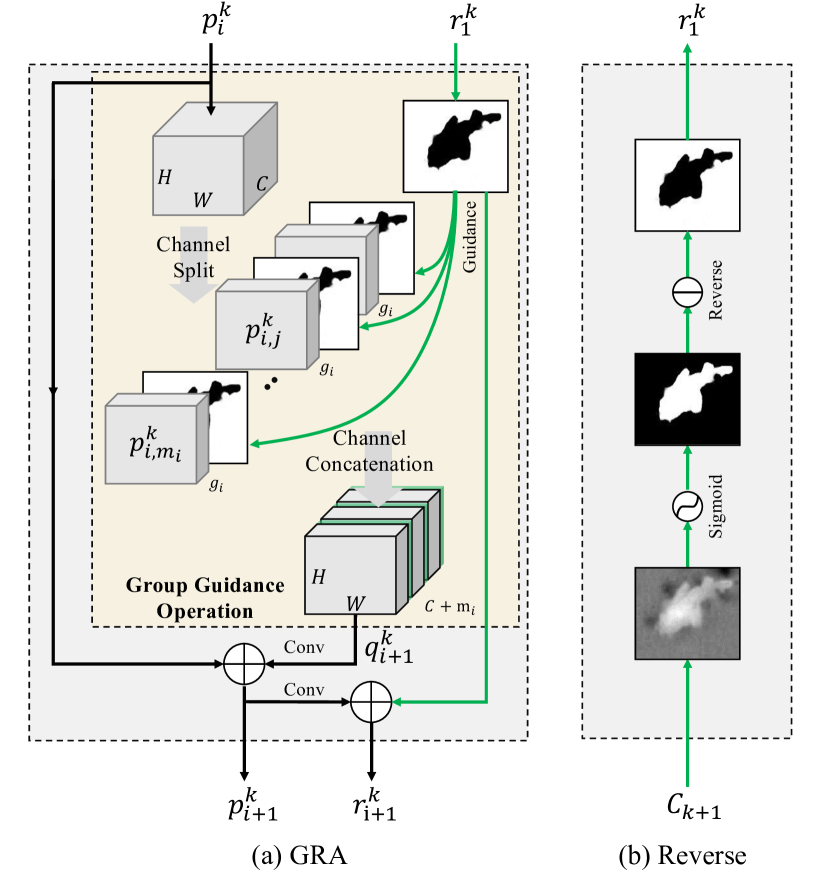
Figure 14: Component details. Details on the group-reversal attention (b) block $G_{i}^{k}$ in the identification phase, where $i$ denotes the number of GRAs in the $k$-th feature pyramids. Note that $m_{i}=C/g_{i}$.

Group Guidance Operation (GGO).   As shown in [7], reverse attention is used for mining complementary regions and details by erasing the existing estimated target regions from side-output features. Inspired by [69], we present a novel group-wise operation to utilize the reverse guidance prior more effectively. As can be seen in Fig. 14 (a), the group guidance operation contains two main steps. First, we split the candidate features $\{p_{i}^{k}\in\mathbb{R}^{H/2^{k}\times W/2^{k}\times C},k=3,4,5\}$ into multiple (i.e., $m_{i}=C/g_{i}$) groups along the channel-wise dimension, where $i=1,2,3$ and $g_{i}$ denotes the group size of processed features. Then, the guidance prior $r_{1}^{k}$ is periodically interpolated among the split features $p_{i,j}^{k}\in\mathbb{R}^{H/2^{k}\times W/2^{k}\times{\color[rgb]{0,0,0}g_{i}}}$, where $i\in\{1,2,3\},j\in\{1,\dots,{\color[rgb]{0,0,0}m_{i}}\},k\in\{3,4,5\}$. Thus, this operation (i.e., $q_{i+1}^{k}=\mathbf{F}^{GGO}[p_{i}^{k},r_{i}^{k};{\color[rgb]{0,0,0}m_{i}}]$) can be decoupled as two steps:

$$\textit{Step I:}~{}\{p_{i,1}^{k},\dots,p_{i,j}^{k},\dots,p_{i,{\color[rgb]{0,0,0}m_{i}}}^{k}\}~{}\leftarrow~{}\mathbf{F}^{S}(p_{i}^{k})$$ (3)

$$\textit{Step II:}~{}q_{i+1}^{k}~{}\leftarrow~{}\mathbf{F}^{C}(\{p_{i,1}^{k},r_{1}^{k}\},\dots,\{p_{i,j}^{k},r_{1}^{k}\},\dots,\{p_{i,{\color[rgb]{0,0,0}m_{i}}}^{k},r_{1}^{k}\}),$$

where $\mathbf{F}^{S}$ and $\mathbf{F}^{C}$ indicate the channel-wise split and concatenation function for the candidates. Note that $\mathbf{F}^{GGO}:p_{i}^{k}\in\mathbb{R}^{H/2^{k}\times W/2^{k}\times C}\rightarrow q_{i+1}^{k}\in\mathbb{R}^{H/2^{k}\times W/2^{k}\times(C+{\color[rgb]{0,0,0}m_{i}})}$, where $k\in\{3,4,5\}$. In contrast, [7] puts more emphasis on ensuring that the candidate features are directly multiplied by the priors, which may incur two issues: a) feature confusion due to the limited discriminative ability of the network, and b) the simple multiplication introduces both true and false guidance priors and is thus prone to accumulating inaccuracies. Compared to [7], our GGO can explicitly isolate the guidance prior and candidate feature before the subsequent refinement process.

Group-Reversal Attention (GRA).   Finally, we introduce the residual learning process, termed the GRA block, with the assistance of both the reverse guidance and group guidance operation. According to previous studies [59, 60], multi-stage refinement can improve performance. We thus combine multiple GRA blocks (e.g., $G^{k}_{i}$, $i\in\{1,2,3\},k\in\{3,4,5\}$) to progressively refine the coarse prediction via different feature pyramids. Overall, each GRA block has three residual learning processes:

1. We combine candidate features $p_{i}^{k}$ and $r_{1}^{k}$ via the group guidance operation and then use the residual stage to produce the refined features $p_{i+1}^{k}$. This is formulated as:

   $$p_{i+1}^{k}=p_{i}^{k}+g[\mathbf{F}^{GGO}[p_{i}^{k},r_{1}^{k};{\color[rgb]{0,0,0}m_{i}}];\mathbf{W}^{v}_{GRA}],$$ (4)

   where $\mathbf{W}^{v}$ denotes the convolutional layer with a 3$\times$3 kernel followed by batch normalization layer for reducing the channel number from $C+m_{i}$ to $C$. Note that we only reverse the guidance prior in the first GRA block (i.e., when $i=1$) in the default implementation. Refer to Section 5.3 for detailed discussion.

2. Then, we get a single channel residual guidance:

   $$r_{i+1}^{k}=r_{1}^{k}+g[p_{i+1}^{k};\mathbf{W}^{w}_{GRA}],$$ (5)

   which is parameterized by learnable weights $\mathbf{W}^{w}_{GRA}$.

3. Finally, we only output the refined guidance, which serves as the residual prediction. It is formulated as:

   $$C_{k}=r_{i+1}^{k}+\delta(C_{k+1}),$$ (6)

   where $\delta(\cdot)$ is $\delta^{2}_{\uparrow}$ when $k=\{3,4\}$ and $\delta^{4}_{\downarrow}$ when $k=5$.

4.4 Implementation Details

4.4.1 Learning Strategy

Our loss function is defined as $\textit{L}=\textit{L}_{IoU}^{W}+\textit{L}_{BCE}^{W}$, where $\textit{L}_{IoU}^{W}$ and $\textit{L}_{BCE}^{W}$ represent the weighted intersection-over-union (IoU) loss and binary cross entropy (BCE) loss for the global restriction and local (pixel-level) restriction. Different from the standard IoU loss, which has been widely adopted in segmentation tasks, the weighted IoU loss increases the weights of hard pixels to highlight their importance. In addition, compared with the standard BCE loss, $\textit{L}_{BCE}^{W}$ pays more attention to hard pixels rather than assigning all pixels equal weights. The definitions of these losses are the same as in [59, 70] and their effectiveness has been validated in the field of salient object detection. Here, we adopt deep supervision for the three side-outputs (i.e., $C_{3}$, $C_{4}$, and $C_{5}$) and the global map $C_{6}$. Each map is up-sampled (e.g., $C_{3}^{up}$) to the same size as the ground-truth map $G$. Thus, the total loss for the proposed SINet can be formulated as: $\textit{L}_{total}=\textit{L}(C_{6}^{up},G)+\sum_{i=3}^{i=5}\textit{L}(C_{i}^{up},G)$.

4.4.2 Hyperparameter Settings

SINet is implemented in PyTorch and trained with the Adam optimizer [71]. During the training stage, the batch size is set to 36, and the learning rate starts at 1e-4, dividing by 10 every 50 epochs. The whole training time is only about 4 hours for 100 epochs. The running time is measured on an Intel^® i9-9820X CPU @3.30GHz $\times$ 20 platform and a single NVIDIA TITAN RTX GPU. During inference, each image is resized to 352$\times$352 and then fed into the proposed pipeline to obtain the final prediction without any post-processing techniques. The inference speed is $\sim$45 fps on a single GPU without I/O time. Both PyTorch [72] and Jittor [73] verisons of the source code will be made publicly avaliable.

TABLE II: Quantitative results on three different datasets. The best scores are highlighted in bold. Note that the ANet-SRM model (only trained on CAMO) does not have a publicly available code, thus other results are not available. $\uparrow$ indicates the higher the score the better. $E_{\phi}$ denotes mean E-measure [74].

	CHAMELEON [24]				CAMO-Test [25]				COD10K-Test (OUR)
Baseline Models	$S_{\alpha}\uparrow$	$E_{\phi}\uparrow$	$F_{\beta}^{w}\uparrow$	$M\downarrow$	$S_{\alpha}\uparrow$	$E_{\phi}\uparrow$	$F_{\beta}^{w}\uparrow$	$M\downarrow$	$S_{\alpha}\uparrow$	$E_{\phi}\uparrow$	$F_{\beta}^{w}\uparrow$	$M\downarrow$
FPN [75]	0.794	0.783	0.590	0.075	0.684	0.677	0.483	0.131	0.697	0.691	0.411	0.075
MaskRCNN [76]	0.643	0.778	0.518	0.099	0.574	0.715	0.430	0.151	0.613	0.748	0.402	0.080
PSPNet [77]	0.773	0.758	0.555	0.085	0.663	0.659	0.455	0.139	0.678	0.680	0.377	0.080
UNet++ [78]	0.695	0.762	0.501	0.094	0.599	0.653	0.392	0.149	0.623	0.672	0.350	0.086
PiCANet [79]	0.769	0.749	0.536	0.085	0.609	0.584	0.356	0.156	0.649	0.643	0.322	0.090
MSRCNN [80]	0.637	0.686	0.443	0.091	0.617	0.669	0.454	0.133	0.641	0.706	0.419	0.073
PFANet [81]	0.679	0.648	0.378	0.144	0.659	0.622	0.391	0.172	0.636	0.618	0.286	0.128
CPD [63]	0.853	0.866	0.706	0.052	0.726	0.729	0.550	0.115	0.747	0.770	0.508	0.059
HTC [82]	0.517	0.489	0.204	0.129	0.476	0.442	0.174	0.172	0.548	0.520	0.221	0.088
ANet-SRM [25]	-	-	-	-	0.682	0.685	0.484	0.126	-	-	-	-
EGNet [12]	0.848	0.870	0.702	0.050	0.732	0.768	0.583	0.104	0.737	0.779	0.509	0.056
PraNet [7]	0.860	0.907	0.763	0.044	0.769	0.824	0.663	0.094	0.789	0.861	0.629	0.045
SINet_cvpr [1]	0.869	0.891	0.740	0.044	0.751	0.771	0.606	0.100	0.771	0.806	0.551	0.051
SINet (OUR)	0.888	0.942	0.816	0.030	0.820	0.882	0.743	0.070	0.815	0.887	0.680	0.037

TABLE III: Quantitative results on four super-classes of the COD10K dataset in terms of four widely used evaluation metrics. All methods are trained using the same dataset as in [1]. $\uparrow$ indicates the higher the score the better, and $\downarrow$: the lower the better.

	Amphibian (124 images)				Aquatic (474 images)				Flying (714 images)				Terrestrial (699 images)
Baseline Models	$S_{\alpha}\uparrow$	$E_{\phi}\uparrow$	$F_{\beta}^{w}\uparrow$	$M\downarrow$	$S_{\alpha}\uparrow$	$E_{\phi}\uparrow$	$F_{\beta}^{w}\uparrow$	$M\downarrow$	$S_{\alpha}\uparrow$	$E_{\phi}\uparrow$	$F_{\beta}^{w}\uparrow$	$M\downarrow$	$S_{\alpha}\uparrow$	$E_{\phi}\uparrow$	$F_{\beta}^{w}\uparrow$	$M\downarrow$
FPN [75]	0.745	0.776	0.497	0.065	0.684	0.732	0.432	0.103	0.726	0.766	0.440	0.061	0.601	0.656	0.353	0.109
MaskRCNN [76]	0.665	0.785	0.487	0.081	0.560	0.721	0.344	0.123	0.644	0.767	0.449	0.063	0.611	0.630	0.380	0.075
PSPNet [77]	0.736	0.774	0.463	0.072	0.659	0.712	0.396	0.111	0.700	0.743	0.394	0.067	0.669	0.718	0.332	0.071
UNet++ [78]	0.677	0.745	0.434	0.079	0.599	0.673	0.347	0.121	0.659	0.727	0.397	0.068	0.608	0.749	0.288	0.070
PiCANet [79]	0.686	0.702	0.405	0.079	0.616	0.631	0.335	0.115	0.663	0.676	0.347	0.069	0.658	0.708	0.273	0.074
MSRCNN [80]	0.722	0.786	0.555	0.055	0.614	0.686	0.398	0.107	0.675	0.744	0.466	0.058	0.594	0.661	0.361	0.081
PFANet [81]	0.693	0.677	0.358	0.110	0.629	0.626	0.319	0.155	0.658	0.648	0.299	0.102	0.611	0.603	0.237	0.111
CPD [63]	0.794	0.839	0.587	0.051	0.739	0.792	0.529	0.082	0.777	0.827	0.544	0.046	0.714	0.771	0.445	0.058
HTC [82]	0.606	0.598	0.331	0.088	0.507	0.495	0.183	0.129	0.582	0.559	0.274	0.070	0.530	0.485	0.170	0.078
EGNet [12]	0.785	0.854	0.606	0.047	0.725	0.793	0.528	0.080	0.766	0.826	0.543	0.044	0.700	0.775	0.445	0.053
PraNet [7]	0.842	0.905	0.717	0.035	0.781	0.883	0.696	0.065	0.819	0.888	0.669	0.033	0.756	0.835	0.565	0.046
SINet_cvpr [1]	0.827	0.866	0.654	0.042	0.758	0.803	0.570	0.073	0.798	0.828	0.580	0.040	0.743	0.778	0.491	0.050
SINet (OUR)	0.858	0.916	0.756	0.030	0.811	0.883	0.696	0.051	0.839	0.908	0.713	0.027	0.787	0.866	0.623	0.039

5 COD Benchmark

5.1 Experimental Settings

5.1.1 Evaluation Metrics

Mean absolute error (MAE) is widely used in SOD tasks. Following Perazzi et al.  [83], we also adopt the MAE ($M$) metric to assess the pixel-level accuracy between a predicted map and ground-truth. However, while useful for assessing the presence and amount of error, the MAE metric is not able to determine where the error occurs. Recently, Fan et al. proposed a human visual perception based E-measure ($E_{\phi}$) [74], which simultaneously evaluates the pixel-level matching and image-level statistics. This metric is naturally suited for assessing the overall and localized accuracy of the concealed object detection results. Note that we report mean $E_{\phi}$ in the experiments. Since concealed objects often contain complex shapes, COD also requires a metric that can judge structural similarity. We therefore utilize the S-measure ($S_{\alpha}$) [84] as our structural similarity evaluation metric. Finally, recent studies [74, 84] have suggested that the weighted F-measure ($F_{\beta}^{w}$) [85] can provide more reliable evaluation results than the traditional $F_{\beta}$. Thus, we further consider this as an alternative metric for COD. Our one-key evaluation code is also available at the project page.

5.1.2 Baseline Models

We select 12 deep learning baselines [75, 76, 77, 78, 79, 80, 81, 63, 82, 12, 25, 7] according to the following criteria: a) classical architectures, b) recently published, and c) achieve SOTA performance in a specific field.

5.1.3 Training/Testing Protocols

For fair comparison with our previous version [1], we adopt the same training settings [1] for the baselines. We evaluate the models on the whole CHAMELEON [24] dataset and the test sets of CAMO and COD10K.

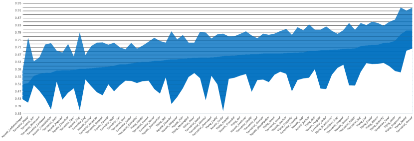
Figure 15: Per-subclass performance. Sub-classes are sorted by difficulty, determined by the mean $S_{\alpha}$ [84] across 12 baselines. We also provide the minimum (bottom line) and maximum (top line) $S_{\alpha}$ for each sub-class.

5.2 Results and Data Analysis

This section provides the quantitative evaluation results on CHAMELEON, CAMO, and COD10K datasets, respectively.

Performance on CHAMELEON.   From Table II, compared with the 12 SOTA object detection baselines and ANet-SRM, our SINet achieves the new SOTA performances across all metrics. Note that our model does not apply any auxiliary edge/boundary features (e.g., EGNet [12], PFANet [81]), pre-processing techniques [86], or post-processing strategies such as [87, 88].

TABLE IV: Results of $S_{\alpha}$ for each sub-class in our COD10K dataset. The best performing method of each category is highlighted in bold.

	HTC	PFANet	MRCNN	BASNet	UNet++	PiCANet	MSRCNN	PoolNet	PSPNet	FPN	EGNet	CPD	PraNet	SINet
Sub-class	[82]	[81]	[76]	[59]	[78]	[79]	[80]	[89]	[77]	[75]	[12]	[63]	[7]	OUR
Amphibian-Frog	0.600	0.678	0.664	0.692	0.656	0.687	0.692	0.732	0.697	0.731	0.745	0.752	0.823	0.837
Amphibian-Toad	0.609	0.697	0.666	0.717	0.689	0.714	0.739	0.786	0.757	0.752	0.812	0.817	0.853	0.870
Aquatic-BatFish	0.546	0.746	0.634	0.749	0.626	0.624	0.637	0.741	0.724	0.764	0.707	0.761	0.879	0.873
Aquatic-ClownFish	0.547	0.519	0.509	0.464	0.548	0.636	0.571	0.626	0.531	0.730	0.632	0.646	0.707	0.787
Aquatic-Crab	0.543	0.661	0.691	0.643	0.630	0.675	0.634	0.727	0.680	0.724	0.760	0.753	0.792	0.815
Aquatic-Crocodile	0.546	0.631	0.660	0.599	0.602	0.669	0.646	0.743	0.636	0.687	0.772	0.761	0.806	0.825
Aquatic-CrocodileFish	0.436	0.572	0.558	0.475	0.559	0.373	0.479	0.693	0.624	0.515	0.709	0.690	0.669	0.746
Aquatic-Fish	0.488	0.622	0.597	0.625	0.574	0.619	0.680	0.703	0.650	0.699	0.717	0.778	0.784	0.834
Aquatic-Flounder	0.403	0.663	0.539	0.633	0.569	0.704	0.570	0.782	0.646	0.695	0.798	0.774	0.835	0.889
Aquatic-FrogFish	0.595	0.768	0.650	0.736	0.671	0.670	0.653	0.719	0.695	0.807	0.806	0.730	0.781	0.894
Aquatic-GhostPipefish	0.522	0.690	0.556	0.679	0.651	0.675	0.636	0.717	0.709	0.744	0.759	0.763	0.784	0.817
Aquatic-LeafySeaDragon	0.460	0.576	0.442	0.481	0.523	0.499	0.500	0.547	0.563	0.507	0.522	0.534	0.587	0.670
Aquatic-Octopus	0.505	0.708	0.598	0.644	0.663	0.673	0.720	0.779	0.723	0.760	0.810	0.812	0.896	0.887
Aquatic-Pagurian	0.427	0.578	0.477	0.607	0.553	0.624	0.583	0.657	0.608	0.638	0.683	0.611	0.615	0.698
Aquatic-Pipefish	0.510	0.553	0.531	0.557	0.550	0.612	0.566	0.625	0.642	0.632	0.681	0.704	0.769	0.781
Aquatic-ScorpionFish	0.459	0.697	0.482	0.686	0.630	0.605	0.600	0.729	0.649	0.668	0.730	0.746	0.766	0.808
Aquatic-SeaHorse	0.566	0.656	0.581	0.664	0.663	0.623	0.657	0.698	0.687	0.715	0.750	0.765	0.810	0.823
Aquatic-Shrimp	0.500	0.574	0.520	0.631	0.586	0.574	0.546	0.605	0.591	0.667	0.647	0.669	0.727	0.735
Aquatic-Slug	0.493	0.581	0.368	0.492	0.533	0.460	0.661	0.732	0.547	0.664	0.777	0.774	0.701	0.729
Aquatic-StarFish	0.568	0.641	0.617	0.611	0.657	0.638	0.580	0.733	0.722	0.756	0.811	0.787	0.779	0.890
Aquatic-Stingaree	0.519	0.721	0.670	0.618	0.571	0.569	0.709	0.733	0.616	0.670	0.741	0.754	0.704	0.815
Aquatic-Turtle	0.364	0.686	0.594	0.658	0.565	0.734	0.762	0.757	0.664	0.745	0.752	0.786	0.773	0.760
Flying-Bat	0.589	0.652	0.611	0.623	0.557	0.638	0.679	0.725	0.657	0.714	0.765	0.784	0.817	0.847
Flying-Bee	0.578	0.579	0.628	0.547	0.588	0.616	0.679	0.670	0.655	0.665	0.737	0.709	0.763	0.777
Flying-Beetle	0.699	0.741	0.693	0.810	0.829	0.780	0.796	0.860	0.808	0.848	0.830	0.887	0.890	0.903
Flying-Bird	0.591	0.628	0.680	0.627	0.643	0.674	0.681	0.735	0.696	0.708	0.763	0.785	0.822	0.835
Flying-Bittern	0.639	0.621	0.703	0.650	0.673	0.741	0.704	0.785	0.701	0.751	0.802	0.838	0.827	0.849
Flying-Butterfly	0.653	0.692	0.697	0.700	0.725	0.714	0.762	0.777	0.736	0.758	0.816	0.818	0.871	0.883
Flying-Cicada	0.640	0.682	0.620	0.729	0.675	0.691	0.708	0.781	0.744	0.733	0.820	0.812	0.845	0.883
Flying-Dragonfly	0.472	0.679	0.624	0.712	0.670	0.694	0.682	0.695	0.681	0.707	0.761	0.779	0.779	0.837
Flying-Frogmouth	0.684	0.766	0.648	0.828	0.813	0.722	0.773	0.883	0.741	0.795	0.901	0.928	0.927	0.941
Flying-Grasshopper	0.563	0.671	0.651	0.689	0.656	0.692	0.666	0.734	0.710	0.740	0.773	0.779	0.821	0.833
Flying-Heron	0.563	0.579	0.629	0.598	0.670	0.647	0.699	0.718	0.654	0.743	0.783	0.786	0.810	0.823
Flying-Katydid	0.540	0.661	0.593	0.657	0.653	0.659	0.615	0.696	0.687	0.709	0.730	0.739	0.802	0.809
Flying-Mantis	0.527	0.622	0.569	0.618	0.614	0.629	0.603	0.661	0.658	0.670	0.696	0.690	0.749	0.775
Flying-Mockingbird	0.641	0.550	0.622	0.593	0.636	0.596	0.664	0.670	0.674	0.683	0.721	0.737	0.788	0.838
Flying-Moth	0.583	0.720	0.726	0.737	0.707	0.685	0.747	0.783	0.753	0.798	0.833	0.854	0.878	0.917
Flying-Owl	0.625	0.671	0.705	0.656	0.657	0.718	0.710	0.781	0.712	0.750	0.793	0.809	0.837	0.868
Flying-Owlfly	0.614	0.690	0.524	0.669	0.633	0.580	0.599	0.778	0.583	0.743	0.782	0.756	0.758	0.863
Other-Other	0.571	0.613	0.603	0.593	0.638	0.653	0.675	0.687	0.671	0.665	0.725	0.700	0.777	0.779
Terrestrial-Ant	0.506	0.516	0.508	0.519	0.523	0.585	0.538	0.552	0.572	0.564	0.627	0.605	0.676	0.669
Terrestrial-Bug	0.578	0.681	0.682	0.687	0.686	0.701	0.691	0.743	0.710	0.799	0.799	0.803	0.828	0.856
Terrestrial-Cat	0.505	0.585	0.591	0.557	0.562	0.608	0.613	0.669	0.624	0.634	0.682	0.678	0.745	0.772
Terrestrial-Caterpillar	0.517	0.643	0.569	0.691	0.636	0.581	0.575	0.638	0.640	0.685	0.684	0.704	0.729	0.776
Terrestrial-Centipede	0.432	0.573	0.476	0.485	0.496	0.554	0.629	0.703	0.561	0.536	0.727	0.643	0.704	0.762
Terrestrial-Chameleon	0.556	0.651	0.627	0.653	0.619	0.619	0.632	0.695	0.659	0.673	0.713	0.732	0.789	0.804
Terrestrial-Cheetah	0.536	0.649	0.699	0.624	0.603	0.662	0.598	0.717	0.720	0.667	0.732	0.769	0.800	0.826
Terrestrial-Deer	0.530	0.581	0.610	0.564	0.558	0.600	0.623	0.650	0.644	0.660	0.667	0.670	0.719	0.757
Terrestrial-Dog	0.572	0.560	0.596	0.536	0.559	0.574	0.614	0.608	0.588	0.613	0.607	0.648	0.666	0.707
Terrestrial-Duck	0.530	0.535	0.557	0.539	0.524	0.558	0.619	0.582	0.602	0.548	0.598	0.682	0.742	0.746
Terrestrial-Gecko	0.485	0.674	0.662	0.725	0.683	0.705	0.606	0.733	0.724	0.747	0.789	0.771	0.833	0.848
Terrestrial-Giraffe	0.469	0.628	0.697	0.620	0.611	0.701	0.635	0.681	0.718	0.722	0.747	0.776	0.809	0.784
Terrestrial-Grouse	0.704	0.760	0.726	0.721	0.774	0.805	0.780	0.879	0.803	0.806	0.904	0.919	0.888	0.921
Terrestrial-Human	0.530	0.629	0.608	0.613	0.549	0.577	0.658	0.697	0.636	0.665	0.708	0.700	0.765	0.817
Terrestrial-Kangaroo	0.482	0.586	0.599	0.467	0.548	0.588	0.571	0.644	0.630	0.623	0.650	0.620	0.798	0.816
Terrestrial-Leopard	0.617	0.647	0.742	0.616	0.640	0.652	0.673	0.736	0.720	0.704	0.744	0.791	0.791	0.823
Terrestrial-Lion	0.534	0.634	0.695	0.599	0.660	0.656	0.658	0.720	0.714	0.663	0.754	0.751	0.805	0.813
Terrestrial-Lizard	0.579	0.629	0.634	0.635	0.633	0.656	0.627	0.710	0.702	0.716	0.744	0.777	0.804	0.830
Terrestrial-Monkey	0.423	0.693	0.724	0.593	0.611	0.730	0.663	0.792	0.678	0.614	0.709	0.699	0.851	0.888
Terrestrial-Rabbit	0.504	0.657	0.685	0.634	0.635	0.721	0.731	0.794	0.722	0.758	0.789	0.806	0.829	0.843
Terrestrial-Reccoon	0.451	0.525	0.536	0.461	0.482	0.702	0.723	0.643	0.532	0.592	0.691	0.659	0.781	0.766
Terrestrial-Sciuridae	0.533	0.612	0.638	0.573	0.608	0.693	0.661	0.745	0.725	0.721	0.775	0.757	0.810	0.842
Terrestrial-Sheep	0.434	0.451	0.721	0.410	0.482	0.467	0.763	0.660	0.466	0.430	0.489	0.487	0.481	0.500
Terrestrial-Snake	0.544	0.590	0.586	0.603	0.567	0.614	0.597	0.714	0.695	0.652	0.738	0.788	0.771	0.831
Terrestrial-Spider	0.528	0.594	0.593	0.594	0.580	0.621	0.572	0.650	0.649	0.651	0.685	0.687	0.740	0.771
Terrestrial-StickInsect	0.473	0.548	0.486	0.526	0.535	0.600	0.491	0.578	0.607	0.629	0.616	0.647	0.660	0.696
Terrestrial-Tiger	0.489	0.583	0.576	0.555	0.573	0.563	0.565	0.638	0.602	0.599	0.647	0.621	0.690	0.703
Terrestrial-Wolf	0.472	0.574	0.602	0.535	0.534	0.568	0.621	0.650	0.656	0.651	0.704	0.662	0.737	0.749
Terrestrial-Worm	0.485	0.652	0.596	0.642	0.628	0.558	0.651	0.692	0.629	0.684	0.763	0.670	0.724	0.806

Performance on CAMO.   We also test our model on the CAMO [25] dataset, which includes various concealed objects. Based on the overall performances reported in Table II, we find that the CAMO dataset is more challenging than CHAMELEON. Again, SINet obtains the best performance, further demonstrating its robustness.

Performance on COD10K.   With the test set (2,026 images) of our COD10K dataset, we again observe that the proposed SINet is consistently better than other competitors. This is because its specially designed search and identification modules can automatically learn rich diversified features from coarse to fine, which are crucial for overcoming challenging ambiguities in object boundaries. The results are shown in Table II and Table III.

Per-subclass Performance.   In addition to the overall quantitative comparisons on our COD10K dataset, we also report the quantitative per-subclass results in the Table IV to investigate the pros and cons of the models for future researchers. In Fig. 15, we additionally show the minimum, mean, and maximum S-measure performance of each sub-class over all baselines. The easiest sub-class is “Grouse”, while the most difficult is the “LeafySeaDragon”, from the aquatic and terrestrial categories, respectively.

Qualitative Results.   We present more detection results of our conference version model (SINet_cvpr) for various challenging concealed objects, such as spider, moth, sea horse, and toad, in the supplementary materials. As shown in Fig. 16, SINet further improves the visual results compared to SINet_cvpr in terms of different lighting ($1^{st}$ row), appearance changes ($2^{nd}$ row), and indefinable boundaries ($3^{rd}$ to $5^{th}$). PFANet [81] is able to locate the concealed objects, but the outputs are always inaccurate. By further using reverse attention module, PraNet [7] achieves a relatively more accurate location than PFANet in the first case. Nevertheless, it still misses the fine details of objects, especially for the fish in the $2^{nd}$ and $3^{rd}$ rows. For all these challenging cases, SINet is able to infer the real concealed object with fine details, demonstrating the robustness of our framework.

GOS vs. SOD Baselines.   One noteworthy finding is that, among the top-3 models, the GOS model (i.e., FPN [75]) performs worse than the SOD competitors, CPD [63], EGNet [12], suggesting that the SOD framework may be better suited for extension to COD tasks. Compared with both the GOS [75, 76, 77, 78, 80, 82] and the SOD [79, 81, 63, 12] models, SINet significantly decrease the training time (e.g., SINet: 4 hours vs. EGNet: 48 hours) and achieve the SOTA performance on all datasets, showing that they are promising solutions for the COD problem. Due to the limited space, fully comparing them with existing SOTA SOD models is beyond the scope of this paper. Note that our main goal is to provide more general observations for future work. More recent SOD models can be found in our project page.

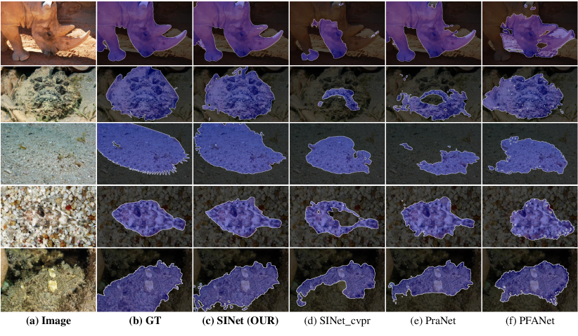
Figure 16: Comparison of our SINet and three top-performing baselines, including (d) SINet_cvpr [1], (e) PraNet [7], and (f) PFANet [81].

TABLE V: Structure-measure ($S_{\alpha}\uparrow$ [84]) scores for cross-dataset generalization. SINet_cvpr is trained on one dataset (rows) and tested on all datasets (columns). “Self”: training and testing on the same dataset (diagonal). “Mean others”: average score on all except self.

	CAMO  [25]	COD10K (OUR)	Self	Mean others	Drop$\downarrow$
CAMO [25]	0.803	0.702	0.803	0.702	12.6%
COD10K (OUR)	0.742	0.700	0.700	0.742	-6.0%
Mean others	0.742	0.702

Generalization.   The generalizability and difficulty of datasets play a crucial role in both training and assessing different algorithms [35]. Hence, we study these aspects for existing COD datasets, using the cross-dataset analysis method [90], i.e., training a model on one dataset, and testing it on others. We select two datasets, namely CAMO [25], and our COD10K. Following [35], for each dataset, we randomly select 800 images as the training set and 200 images as the testing set. For fair comparison, we train SINet_cvpr on each dataset until the loss is stable.

TABLE VI: Ablation studies for each component on three test datasets. For details please refer to Section 5.3.

	Decoder		TEM		GRA		CHAMELEON [24]				CAMO-Test [25]				COD10K-Test (OUR)
No.	PD	NCD	Sy. Conv.	Asy. Conv,	Reverse	Group Size	$S_{\alpha}\uparrow$	$E_{\phi}\uparrow$	$F_{\beta}^{w}\uparrow$	$M\downarrow$	$S_{\alpha}\uparrow$	$E_{\phi}\uparrow$	$F_{\beta}^{w}\uparrow$	$M\downarrow$	$S_{\alpha}\uparrow$	$E_{\phi}\uparrow$	$F_{\beta}^{w}\uparrow$	$M\downarrow$
#1				$\checkmark$	$\{1,0,0\}$	$\{32;8;1\}$	0.884	0.940	0.811	0.033	0.812	0.869	0.730	0.073	0.812	0.884	0.679	0.039
#2	$\checkmark$			$\checkmark$	$\{1,0,0\}$	$\{32;8;1\}$	0.881	0.934	0.799	0.034	0.820	0.877	0.740	0.071	0.813	0.884	0.673	0.038
#3		$\checkmark$			$\{1,0,0\}$	$\{32;8;1\}$	0.887	0.934	0.813	0.033	0.811	0.867	0.731	0.074	0.815	0.888	0.680	0.036
#4		$\checkmark$	$\checkmark$		$\{1,0,0\}$	$\{32;8;1\}$	0.888	0.944	0.818	0.030	0.810	0.866	0.730	0.073	0.814	0.883	0.678	0.037
#5		$\checkmark$		$\checkmark$	$\{0,0,0\}$	$\{32;8;1\}$	0.886	0.942	0.814	0.031	0.814	0.873	0.739	0.073	0.814	0.887	0.682	0.037
#6		$\checkmark$		$\checkmark$	$\{1,1,0\}$	$\{32;8;1\}$	0.879	0.928	0.794	0.035	0.820	0.877	0.738	0.071	0.807	0.878	0.661	0.040
#7		$\checkmark$		$\checkmark$	$\{1,1,1\}$	$\{32;8;1\}$	0.886	0.939	0.812	0.031	0.817	0.875	0.736	0.073	0.810	0.884	0.670	0.037
#8		$\checkmark$		$\checkmark$	$\{1,0,0\}$	$\{1;1;1\}$	0.888	0.940	0.812	0.031	0.819	0.877	0.741	0.072	0.814	0.887	0.681	0.037
#9		$\checkmark$		$\checkmark$	$\{1,0,0\}$	$\{8;8;8\}$	0.886	0.943	0.814	0.032	0.816	0.872	0.738	0.074	0.815	0.886	0.682	0.037
#10		$\checkmark$		$\checkmark$	$\{1,0,0\}$	$\{32;32;32\}$	0.884	0.944	0.810	0.033	0.819	0.876	0.738	0.071	0.813	0.884	0.675	0.037
#11		$\checkmark$		$\checkmark$	$\{1,0,0\}$	$\{1;8;32\}$	0.883	0.940	0.812	0.032	0.811	0.869	0.734	0.073	0.815	0.887	0.679	0.036
#OUR		$\checkmark$		$\checkmark$	$\{1,0,0\}$	$\{32;8;1\}$	0.888	0.942	0.816	0.030	0.820	0.882	0.743	0.070	0.815	0.887	0.680	0.037

Table V provides the S-measure results for the cross-dataset generalization. Each row lists a model that is trained on one dataset and tested on all others, indicating the generalizability of the dataset used for training. Each column shows the performance of one model tested on a specific dataset and trained on all others, indicating the difficulty of the testing dataset. Please note that the training/testing settings are different from those used in Table II, and thus the performances are not comparable. As expected, we find that our COD10K has better generalization ability than the CAMO (e.g., the last column ‘Drop$\downarrow$: -6.0%’). This is because our dataset contains a variety of challenging concealed objects (Section 3). We can thus see that our COD10K dataset contains more challenging scenes.

5.3 Ablation Studies

We now provide a detailed analysis of the proposed SINet on CHAMELEON, CAMO, and COD10K. We verify the effectiveness by decoupling various sub-components, including the NCD, TEM, and GRA, as summarized in Table VI. Note that we maintain the same hyperparameters mentioned in Section 4.4 during the re-training process for each ablation variant.

Effectiveness of NCD.   We explore the influence of the decoder in the search phase of our SINet. To verify its necessity, we retrain our network without the NCD (No.#1) and find that, compared with #OUR (last row in Table VI), the NCD is attributed to boosting the performance on CAMO, increasing the mean $E_{\phi}$ score from 0.869 to 0.882. Further, we replace the NCD with the partial decoder [63] (i.e., PD of No.#2) to test the performance of this scheme. Comparing No.#2 with #OUR, our design can enhance the performance slightly, increasing it by 1.7% in terms of $F^{w}_{\beta}$ on the CHAMELEON.

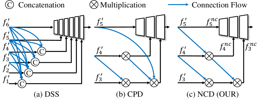
Figure 17: Comparison of various types of inter-layer feature aggregation strategies with a short connection. (a) DSS [32] introduce the densely connected short connection in a top-down manner. (b) CPD [63] constructs a partial decoder by discarding larger resolution features of shallower layers for memory and speed enhancement. (c) Our neighbor connection decoder only propagates between neighboring layers.

As shown in Fig. 17, we present a novel feature aggregation strategy before the modified UNet-like decoder (removing the bottom-two high-resolution layers), termed the NCD, with neighbor connections between adjacent layers. This design is motivated by the fact that the high-level features are superior to semantic strength and location accuracy, but introduce noise and blurred edges for the target object.

Instead of broadcasting features from densely connected layers with a short connection [32] or a partial decoder with a skip connection [63], our NCD exploits the semantic context through a neighbor connection, providing a simple but effective way to reduce inconsistency between different features. Aggregating all features by a short connection [32] increases the parameters. This is one of the major differences between DSS (Fig. 17 a) and NCD. Compared to CPD [63] (Fig. 17 b), which ignores feature transparency between $f_{5}^{\prime}$ and $f_{4}^{\prime}$, NCD is more efficient at broadcasting the features step by step.

Effectiveness of TEM.   We provide two different variants: (a) without TEM (No.#3), and (b) with symmetric convolutional layers [64] (No.#4). Comparing with No.#3, we find that our TEM with asymmetric convolutional layers (No.#OUR) is necessary for increasing the performance on the CAMO dataset. Besides, replacing the standard symmetric convolutional layer (No.#4) with an asymmetric convolutional layer (No.#OUR) has little impact on the learning capability of the network, while further increasing the mean $E_{\phi}$ from 0.866 to 0.882 on the CAMO dataset.

Effectiveness of GRA.   Reverse Guidance. As shown in the ‘Reverse’ column of Table VI, {*,*,*} indicates whether the guidance is reversed (see Fig. 14 (b)) before each GRA block $G^{k}_{i}$. For instance, {1,0,0} means that we only reverse the guidance in the first block (i.e., $r^{k}_{1}$) and the remaining two blocks (i.e., $r^{k}_{2}$ and $r^{k}_{3}$) do not have a reverse operation.

We investigate the contribution of the reverse guidance in the GRA, including three alternatives: (a) without any reverse, i.e., {0,0,0} of No.#5, (b) reversing the first two guidances $r^{k}_{i},i\in\{1,2\}$, i.e., {1,1,0} of No.#6, and (c) reversing all the guidances $r^{k}_{i},i\in\{1,2,3\}$, i.e., {1,1,1} of No.#7. Compared to the default implementation of SINet (i.e., {1,0,0} of No.#OUR), we find that only reversing the first guidance may help the network to mine diversified representations from two perspectives (i.e., attention and reverse attention regions), while introducing reverse guidance several times in the intermediate process may cause confusion during the learning procedure, especially for setting #6 on the CHAMELEON and COD10K datasets.

Group Size of GGO. As shown in the ‘Group Size’ column of  Table VI, $\{*;*;*\}$ indicates the number of feature slices (i.e., group size $g_{i}$) from the GGO of the first block $G^{k}_{1}$ to last block $G^{k}_{3}$. For example, $\{32;8;1\}$ indicates that we split the candidate feature $p^{k}_{i},i\in\{1,2,3\}$ into 32, 8, and 1 group sizes at each GRA block $G^{k}_{i},i\in\{1,2,3\}$, respectively. Here, we discuss two ways of selecting the group size, i.e., the uniform strategy (i.e., $\{1;1;1\}$ of #8, $\{8;8;8\}$ of #9, $\{32;32;32\}$ of #10) and progressive strategy (i.e., $\{1;8;32\}$ of #11 and $\{32;8;1\}$ of #OUR). We observe that our design based on the progressive strategy can effectively maintain the generalizability of the network, providing more satisfactory performance compared with other variants.

6 Downstream Applications

Concealed object detection systems have various downstream applications in fields such as medicine, art, and agriculture. Here, we envision some potential uses due to the common feature of these applications where the target objects share similar appearance with the background. Under such circumstances, COD models are very suitable to act as a core component of these applications to mine camouflaged objects. Note that these applications are only toy examples to spark interesting ideas for future research.

6.1 Application I: Medicine

6.1.1 Polyp Segmentation

As we all know, early diagnosis through medical imaging plays a key role in the treatment of diseases. However, the early disease area/lesions usually have a high degree of homogeneity with the surrounding tissues. As a result, it is difficult for doctors to identity the lesion area in the early stage from a medical image. One typical example is the early colonoscopy to segment polyps, which has contributed to roughly 30% decline in the incidence of colorectal cancer [7]. Similar to concealed object detection, polyp segmentation (see Fig. 18) also faces several challenges, such as variation in appearance and blurred boundaries. The recent state-of-the-art polyp segmentation model, PraNet [7], has shown promising performance in both polyp segmentation (Top-1) and concealed object segmentation (Top-2). From this point of view, embedding our SINet into this application could potentially achieve more robust results.

\begin{overpic}[width=433.62pt]{Medical-min} \put(10.0,-3.0){(a)} \put(35.0,-3.0){(b)} \put(62.0,-3.0){(c)} \put(85.0,-3.0){(d)} \end{overpic}

Figure 18: Polyp segmentation. (a) & (c) are input polyp images. (b) & (d) are corresponding ground-truths.

\begin{overpic}[width=433.62pt]{Medical-2-min} \put(10.0,-3.0){(a)} \put(35.0,-3.0){(b)} \put(62.0,-3.0){(c)} \put(85.0,-3.0){(d)} \end{overpic}

Figure 19: Lung infection segmentation. The first row presents COVID-19 lung infection CT scans, while the second row shows their ground-truths labeled by doctors. From (a) to (d), COVID-19 patients from mild to severe.

\begin{overpic}[width=433.62pt]{SurfaceDefect-min} \put(10.0,-3.0){(a)} \put(35.0,-3.0){(b)} \put(62.0,-3.0){(c)} \put(85.0,-3.0){(d)} \end{overpic}

Figure 20: Surface defect detection. The defect types are textile (a), stone (b), magnetic tile (c), and wood (d), respectively. The second row presented their corresponding ground truths. Source images are derived from [91].

6.1.2 Lung Infection Segmentation

Another concealed object detection example is the lung infection segmentation task in the medical field. Recently, COVID-19 has been of particular concern, and resulted in a global pandemic. An AI system equipped with a COVID-19 lung infection segmentation model would be helpful in the early screening of COVID-19. More details on this application can be found in the recent segmentation model [8] and survey paper [92]. We believe retrain our SINet model using COVID-19 lung infection segmentation datasets will be another interesting potential application.

6.2 Application II: Manufacturing

6.2.1 Surface Defect Detection

In industrial manufacturing, products (e.g., wood, textile, and magnetic tile) of poor quality will inevitably lead to adverse effects on the economy. As can be seen from Fig. 20, the surface defects are challenging, with different factors including low contrast, ambiguous boundaries and so on. Since traditional surface defect detection systems mainly rely on humans, major issues are highly subjective and time-consuming to identify. Thus, designing an automatic recognition system based on AI is essential to increase productivity. We are actively constructing such a data set to advance related research. Some related papers can be found at: https://github.com/Charmve/Surface-Defect-Detection/tree/master/Papers.

\begin{overpic}[width=433.62pt]{PestsDetection-min} \put(14.0,-3.0){(a)} \put(48.0,-3.0){(b)} \put(81.0,-3.0){(c)} \end{overpic}

Figure 21: Pest detection. For pest detection applications, the system can generate a bounding box (b) for each locally screened image (a) or provide statistics (pest counting) for locust plague density monitoring in the whole environment (c).

\begin{overpic}[width=433.62pt]{FruitMaturity-min} \put(14.0,-3.0){(a)} \put(48.0,-3.0){(b)} \put(81.0,-3.0){(c)} \end{overpic}

Figure 22: Fruit maturity detection. Compared with the traditional manual inspection (c) of fruits, such as Persea Americana (a) and Myrica Rubra (b) for maturity, an AI-based maturity monitoring system will greatly improve production efficiency.

6.3 Application III: Agriculture

6.3.1 Pest Detection

Since early 2020, plagues of desert locusts have invaded the world, from Africa to South Asia. Large numbers of locusts gnaw on fields and completely destroy agricultural products, causing serious financial losses and famine due to food shortages. As shown in Fig. 21, introducing AI-based techniques to provide scientific monitoring is feasible for achieving sustainable regulation/containment by governments. Collecting relevant insect data for COD models requires rich biological knowledge, which is also a difficulty faced in this application.

6.3.2 Fruit Maturity Detection

In the early stages of ripening, many fruits appear similar to green leaves, making it difficult for farmers to monitor production. We present two types of fruits, i.e., Persea Americana and Myrica Rubra, in Fig. 22. These fruits share similar characteristics to concealed objects, so it is possible to utilize a COD algorithm to identify them and improve the monitoring efficiency.

Figure 23: Recreational art. Some animals are embedded into the background by algorithms. Source images from Chu et al.  [9] and all rights reserved by 2010 John Van Straalen.

6.4 Application IV: Art

6.4.1 Recreational Art

Background warping to concealed salient objects is a fascinating technique in the SIGGRAPH community. Fig. 23 presents some examples generated by Chu et al. in [9]. We argue that this technique will provide more training data for existing data-hungry deep learning models, and thus it is of value to explore the underlying mechanism behind the feature search and conjunction search theory described by Treisman and Wolfe [93, 94].

\begin{overpic}[width=433.62pt]{Concealed2Salient} \put(14.0,-3.0){(a)} \put(48.0,-3.0){(b)} \put(81.0,-3.0){(c)} \end{overpic}

Figure 24: Converting concealed objects to salient objects. Source images from [25]. One interesting application is to identify (b) a specific concealed object (a) and then convert it to a salient object (c).

\begin{overpic}[width=433.62pt]{TransparentObject-min} \put(14.0,-3.0){(a)} \put(48.0,-3.0){(b)} \put(81.0,-3.0){(c)} \end{overpic}

Figure 25: Transparent stuff/objects detection. In our daily lives, we humans see, touch, or interact with various transparent stuff such as windows (a), glass doors (b), and glass walls (c). Second rows are corresponding ground-truths. It is essential to teach AI robots to identify transparent stuff/objects to avoid unseen obstacles.

\begin{overpic}[width=433.62pt]{SearchEngine} \put(0.0,5.0){(b)} \put(0.0,25.0){(a)} \end{overpic}

Figure 26: Search engines. Internet search engine application equipped without (a)/with (b) a concealed detection system.

6.4.2 From Concealed to Salient Objects

Concealed object detection and salient object detection are two opposite tasks, making it convenient for us to design a multi-task learning framework that can simultaneously increase the robustness of the network. As shown in Fig. 24, there exist two reverse objects (a) and (c). An interesting application is to provide a scroll bar to allow users to customize the degree of salient objects from the concealed objects.

6.5 Application V: Daily Life

6.5.1 Transparent Stuff/Objects Detection

Transparent objects, such as glass products, are commonplace in our daily life. These objects/things, including doors and walls, inherit the appearance of their background, making them unnoticeable, as illustrated in Fig. 25. As a sub-task of concealed object detection, transparent object detection [47] and transparent object tracking [95] have shown promise.

6.5.2 Search Engines

Fig. 26 shows an example of search results from Google. From the results (Fig. 26 a), we notice that the search engine cannot detect the concealed butterfly, and thus only provides images with similar backgrounds. Interestingly, when the search engine is equipped with a concealed detection system (here, we just simply change the keyword), it can identify the concealed object and then feedback several butterfly images (Fig. 26 b).

7 Potential Research Directions

Despite the recent 10 years of progress in the field of concealed object detection, the leading algorithms in the deep learning era remain limited compared to those for generic object detection [96] and cannot yet effectively solve real-world challenges as shown in our COD10K benchmark (Top-1: $F_{\beta}^{w}<0.7$). We highlight some long-standing challenges, as follows:

• Concealed object detection under limited conditions: few/zero-shot learning, weakly supervised learning, unsupervised learning, self-supervised learning, limited training data, unseen object class, etc.

• Concealed object detection combined with other modalities: Text, Audio, Video, RGB-D, RGB-T, 3D, etc.

• New directions based on the rich annotations provided in the COD10K, such as concealed instance segmentation, concealed edge detection, concealed object proposal, concealed object ranking, among others.

Based on the above-mentioned challenges, there are a number of foreseeable directions for future research:

(1) Weakly/Semi-Supervised Detection: Existing deep-based methods extract the features in a fully supervised manner from images annotated with object-level labels. However, the pixel-level annotations are usually manually marked by LabelMe or Adobe Photoshop tools with intensive professional interaction. Thus, it is essential to utilize weakly/semi (partially) annotated data for training in order to avoid heavy annotation costs.

(2) Self-Supervised Detection: Recent efforts to learn representations (e.g., image, audio, and video) using self-supervised learning [97, 98] have achieved world-renowned achievements, attracting much attention. Thus, it is natural to setup a self-supervised learning benchmark for the concealed object detection task.

(3) Concealed Object Detection in Other Modalities: Existing concealed data is only based on static images or dynamic videos [99]. However, concealed object detection in other modalities can be closely related in domains such as pest monitoring in the dark night, robotics, and artist design. Similar to in RGB-D SOD [53], RGB-T SOD [100], CoSOD [101, 102], and VSOD [103], these modalities can be audio, thermal, group image, or depth data, raising new challenges under specific scenes.

(4) Concealed Object Classification: Generic object classification is a fundamental task in computer vision. Thus concealed object classification will also likely gain attention in the future. By utilizing the class and sub-class labels provided in COD10K, one could build a large scale and fine-grain classification task.

(5) Concealed Object Proposal and Tracking: In this paper, the concealed object detection is actually a segmentation task. It is different from traditional object detection, which generates a proposal or bounding boxes as the prediction. As such, concealed object proposal and tracking is a new and interesting direction [104] for future work.

(6) Concealed Object Ranking: Currently, most concealed object detection algorithms are built upon binary ground-truths to generate the masks of concealed objects, with only limited works analyzing the rank of concealed objects [39]. However, understanding the level of concealment could help to better explore the mechanism behind the models, providing deeper insights into them. We refer readers to [105, 39] for some inspiring ideas.

(7) Concealed Instance Segmentation: As described in [20], instance segmentation is more crucial than object-level segmentation for practical applications. For example, we can push the research on camouflaged object segmentation into camouflaged instance segmentation.

(8) Universal Network for Multiple Tasks: As studied by Zamir et al. in Taskonomy [21], different visual tasks have strong relationships. Thus, their supervision can be reused in one universal system without piling up complexity. It is natural to consider devising a universal network to simultaneously localize, segment and rank concealed objects.

(9) Neural Architecture Search: Both traditional algorithms and deep learning-based models for concealed object detection require human experts with strong prior knowledge or skilled expertise. Sometimes, the hand-crafted features and architectures designed by algorithm engineers may not optimal. Therefore, neural architecture search techniques, such as the popular automated machine learning [106], offer a potential direction.

(10) Transferring Salient Objects to Concealed Objects: Due to space limitations, we only evaluated typical salient object detection models in our benchmark section. There are several valuable problems that deserve further studying, however, such as transferring salient objects to concealed objects to increase the training data, and introducing a generative adversarial mechanism between the SOD and COD tasks to increase the feature extraction ability of the network.

The ten new research directions listed for concealed object remain far from being solved. However, there are many famous works that can be referred to, providing us a solid basis for studying the object detection task from a concealed perspective.

8 Conclusion

We have presented the first comprehensive study on object detection from a concealed vision perspective. Specifically, we have provided the new challenging and densely annotated COD10K dataset, conducted a large-scale benchmark, developed a simple but efficient end-to-end search and identification framework (i.e., SINet), and highlighted several potential applications. Compared with existing cutting-edge baselines, our SINet is competitive and generates more visually favorable results. The above contributions offer the community an opportunity to design new models for the COD task. In the future, we plan to extend our COD10K dataset to provide inputs of various forms, such as multi-view images (e.g., RGB-D SOD [107, 108]), textual descriptions, video (e.g., VSOD [103]), among others. We also plan to automatically search the optimal receptive fields [109] and employ improved feature representations [110] for better model performance.

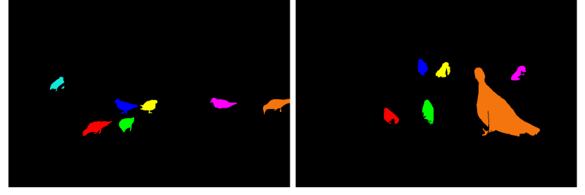
Figure 27: Ground-truths of the images presented in Fig. 1

Deng-Ping Fan received his PhD degree from the Nankai University in 2019. He joined Inception Institute of AI in 2019. He has published about 25 top journal and conference papers such as TPAMI, CVPR, ICCV, ECCV, etc. His research interests include computer vision and visual attention, especially on RGB salient object detection (SOD), RGB-D SOD, Video SOD, Co-SOD. He won the Best Paper Finalist Award at IEEE CVPR 2019, the Best Paper Award Nominee at IEEE CVPR 2020.

Ge-Peng Ji is currently a MS of Communication and Information System at School of Computer Science, Wuhan University. His research interests lie in designing deep neural networks and applying deep learning in various fields of low-level vision, such as RGB salient object detection, RGB-D salient object detection, video object segmentation, concealed object detection, and medical image segmentation.

Ming-Ming Cheng received his PhD degree from Tsinghua University in 2012. He then he did 2 years research fellow, with Prof. Philip Torr in Oxford. He is a full professor at Nankai University since 2016, leading the Media Computing Lab. His research interests includes computer graphics, machine learning, computer vision, and image processing. He is an Associate Editor of IEEE TIP. He received several research awards, including the ACM China Rising Star Award, the IBM Global SUR Award, etc.

Ling Shao is the CEO and the Chief Scientist of the Inception Institute of Artificial Intelligence (IIAI), Abu Dhabi, United Arab Emirates. He was the initiator and the Founding Provost and Executive Vice President of the Mohamed bin Zayed University of Artificial Intelligence (the world’s first AI University), UAE. His research interests include computer vision, machine learning, and medical imaging. He is a fellow of the IEEE, the IAPR, the IET, and the BCS.

References

- [1] D.-P. Fan, G.-P. Ji, G. Sun, M.-M. Cheng, J. Shen, and L. Shao, “Camouflaged object detection,” in IEEE Conf. Comput. Vis. Pattern Recog., 2020, pp. 2777–2787.
- [2] I. C. Cuthill, M. Stevens, J. Sheppard, T. Maddocks, C. A. Párraga, and T. S. Troscianko, “Disruptive coloration and background pattern matching,” Nature, vol. 434, no. 7029, p. 72, 2005.
- [3] A. Owens, C. Barnes, A. Flint, H. Singh, and W. Freeman, “Camouflaging an object from many viewpoints,” in IEEE Conf. Comput. Vis. Pattern Recog., 2014, pp. 2782–2789.
- [4] M. Stevens and S. Merilaita, “Animal camouflage: current issues and new perspectives,” Phil. Trans. R. Soc. B: Biological Sciences, vol. 364, no. 1516, pp. 423–427, 2008.
- [5] A. Kirillov, K. He, R. Girshick, C. Rother, and P. Dollár, “Panoptic segmentation,” in IEEE Conf. Comput. Vis. Pattern Recog., 2019, pp. 9404–9413.
- [6] T. Troscianko, C. P. Benton, P. G. Lovell, D. J. Tolhurst, and Z. Pizlo, “Camouflage and visual perception,” Phil. Trans. R. Soc. B: Biological Sciences, vol. 364, no. 1516, pp. 449–461, 2008.
- [7] D.-P. Fan, G.-P. Ji, T. Zhou, G. Chen, H. Fu, J. Shen, and L. Shao, “Pranet: Parallel reverse attention network for polyp segmentation,” in Med. Image. Comput. Comput. Assist. Interv., 2020.
- [8] D.-P. Fan, T. Zhou, G.-P. Ji, Y. Zhou, G. Chen, H. Fu, J. Shen, and L. Shao, “Inf-Net: Automatic COVID-19 Lung Infection Segmentation from CT Images,” IEEE Trans. Med. Imaging, 2020.
- [9] H.-K. Chu, W.-H. Hsu, N. J. Mitra, D. Cohen-Or, T.-T. Wong, and T.-Y. Lee, “Camouflage images.” ACM Trans. Graph., vol. 29, no. 4, pp. 51–1, 2010.
- [10] Z.-Q. Zhao, P. Zheng, S.-t. Xu, and X. Wu, “Object detection with deep learning: A review,” IEEE T. Neural Netw. Learn. Syst., vol. 30, no. 11, pp. 3212–3232, 2019.
- [11] D.-P. Fan, J. Zhang, G. Xu, M.-M. Cheng, and L. Shao, “Salient objects in clutter,” arXiv preprint arXiv:, 2021.
- [12] J.-X. Zhao, J.-J. Liu, D.-P. Fan, Y. Cao, J. Yang, and M.-M. Cheng, “Egnet:edge guidance network for salient object detection,” in Int. Conf. Comput. Vis., 2019.
- [13] M. Everingham, L. Van Gool, C. K. Williams, J. Winn, and A. Zisserman, “The pascal visual object classes (voc) challenge,” Int. J. Comput. Vis., vol. 88, no. 2, pp. 303–338, 2010.
- [14] J. Deng, W. Dong, R. Socher, L.-J. Li, K. Li, and L. Fei-Fei, “Imagenet: A large-scale hierarchical image database,” in IEEE Conf. Comput. Vis. Pattern Recog., 2009, pp. 248–255.
- [15] T.-Y. Lin, M. Maire, S. Belongie, J. Hays, P. Perona, D. Ramanan, P. Dollár, and C. L. Zitnick, “Microsoft coco: Common objects in context,” in Eur. Conf. Comput. Vis., 2014, pp. 740–755.
- [16] B. Zhou, H. Zhao, X. Puig, S. Fidler, A. Barriuso, and A. Torralba, “Scene parsing through ade20k dataset,” in IEEE Conf. Comput. Vis. Pattern Recog., 2017, pp. 633–641.
- [17] F. Perazzi, J. Pont-Tuset, B. McWilliams, L. Van Gool, M. Gross, and A. Sorkine-Hornung, “A benchmark dataset and evaluation methodology for video object segmentation,” in IEEE Conf. Comput. Vis. Pattern Recog., 2016, pp. 724–732.
- [18] L. Liu, W. Ouyang, X. Wang, P. Fieguth, J. Chen, X. Liu, and M. Pietikäinen, “Deep learning for generic object detection: A survey,” Int. J. Comput. Vis., 2019.
- [19] G. Medioni, “Generic object recognition by inference of 3-d volumetric,” Object Categorization: Comput. Hum. Vis. Perspect., vol. 87, 2009.
- [20] G. Li, Y. Xie, L. Lin, and Y. Yu, “Instance-level salient object segmentation,” in IEEE Conf. Comput. Vis. Pattern Recog., 2017, pp. 247–256.
- [21] A. R. Zamir, A. Sax, W. Shen, L. J. Guibas, J. Malik, and S. Savarese, “Taskonomy: Disentangling task transfer learning,” in IEEE Conf. Comput. Vis. Pattern Recog., 2018, pp. 3712–3722.
- [22] K. Saenko, B. Kulis, M. Fritz, and T. Darrell, “Adapting visual category models to new domains,” in Eur. Conf. Comput. Vis., 2010, pp. 213–226.
- [23] Y. Zhang, L. Gong, L. Fan, P. Ren, Q. Huang, H. Bao, and W. Xu, “A late fusion cnn for digital matting,” in IEEE Conf. Comput. Vis. Pattern Recog., 2019, pp. 7469–7478.
- [24] P. Skurowski, H. Abdulameer, J. Błaszczyk, T. Depta, A. Kornacki, and P. Kozieł, “Animal camouflage analysis: Chameleon database,” 2018, unpublished Manuscript.
- [25] T.-N. Le, T. V. Nguyen, Z. Nie, M.-T. Tran, and A. Sugimoto, “Anabranch network for camouflaged object segmentation,” Comput. Vis. Image Underst., vol. 184, pp. 45–56, 2019.
- [26] J. Shotton, J. Winn, C. Rother, and A. Criminisi, “Textonboost: Joint appearance, shape and context modeling for multi-class object recognition and segmentation,” in Eur. Conf. Comput. Vis., 2006, pp. 1–15.
- [27] C. Liu, J. Yuen, and A. Torralba, “Sift flow: Dense correspondence across scenes and its applications,” IEEE Trans. Pattern Anal. Mach. Intell., vol. 33, no. 5, pp. 978–994, 2010.
- [28] M. Everingham, S. A. Eslami, L. Van Gool, C. K. Williams, J. Winn, and A. Zisserman, “The PASCAL visual object classes challenge: A retrospective,” Int. J. Comput. Vis., vol. 111, no. 1, pp. 98–136, 2015.
- [29] L. Itti, C. Koch, and E. Niebur, “A model of saliency-based visual attention for rapid scene analysis,” IEEE Trans. Pattern Anal. Mach. Intell., vol. 20, no. 11, pp. 1254–1259, 1998.
- [30] M.-M. Cheng, N. J. Mitra, X. Huang, P. H. S. Torr, and S.-M. Hu, “Global contrast based salient region detection,” IEEE Trans. Pattern Anal. Mach. Intell., vol. 37, no. 3, pp. 569–582, 2015.
- [31] S.-H. Gao, Y.-Q. Tan, M.-M. Cheng, C. Lu, Y. Chen, and S. Yan, “Highly efficient salient object detection with 100k parameters,” in Eur. Conf. Comput. Vis., 2020.
- [32] Q. Hou, M.-M. Cheng, X. Hu, A. Borji, Z. Tu, and P. Torr, “Deeply supervised salient object detection with short connections,” IEEE Trans. Pattern Anal. Mach. Intell., vol. 41, no. 4, pp. 815–828, 2019.
- [33] X. Qin, D.-P. Fan, C. Huang, C. Diagne, Z. Zhang, A. C. Sant’Anna, A. Su‘arez, M. Jagersand, and L. Shao, “Boundary-aware segmentation network for mobile and web applications,” arXiv preprint arXiv:2101.04704, 2021.
- [34] A. Borji, M.-M. Cheng, H. Jiang, and J. Li, “Salient object detection: A benchmark,” IEEE Trans. Image Process., vol. 24, no. 12, pp. 5706–5722, 2015.
- [35] W. Wang, Q. Lai, H. Fu, J. Shen, and H. Ling, “Salient object detection in the deep learning era: An in-depth survey,” IEEE Trans. Pattern Anal. Mach. Intell., 2021.
- [36] A. Borji, M.-M. Cheng, Q. Hou, H. Jiang, and J. Li, “Salient object detection: A survey,” Computational Visual Media, vol. 5, no. 2, pp. 117–150, 2019.
- [37] G. H. Thayer and A. H. Thayer, Concealing-coloration in the Animal Kingdom: An Exposition of the Laws of Disguise Through Color and Pattern: Being a Summary of Abbott H. Thayer’s Discoveries. Macmillan Company, 1909.
- [38] H. B. Cott, Adaptive coloratcottion in animals. Methuen & Co., Ltd., 1940.
- [39] Q. Zhai, X. Li, F. Yang, C. Chen, H. Cheng, and D.-P. Fan, “Mutual graph learning for camouflaged object detection,” in IEEE Conf. Comput. Vis. Pattern Recog., 2021.
- [40] Y. Lyu, J. Zhang, Y. Dai, L. Aixuan, B. Liu, N. Barnes, and D.-P. Fan, “Simultaneously localize, segment and rank the camouflaged objects,” in IEEE Conf. Comput. Vis. Pattern Recog., 2021.
- [41] H. Mei, G.-P. Ji, Z. Wei, X. Yang, X. Wei, and D.-P. Fan, “Camouflaged object segmentation with distraction mining,” in IEEE Conf. Comput. Vis. Pattern Recog., 2021.
- [42] D. Tabernik, S. Šela, J. Skvarč, and D. Skočaj, “Segmentation-based deep-learning approach for surface-defect detection,” J. Intell. Manuf., vol. 31, no. 3, pp. 759–776, 2020.
- [43] Y. He, K. Song, Q. Meng, and Y. Yan, “An end-to-end steel surface defect detection approach via fusing multiple hierarchical features,” IEEE Trans. Instrum. Meas., vol. 69, no. 4, pp. 1493–1504, 2020.
- [44] H. Dong, K. Song, Y. He, J. Xu, Y. Yan, and Q. Meng, “Pga-net: Pyramid feature fusion and global context attention network for automated surface defect detection,” IEEE Trans. Industr. Inform., 2020.
- [45] A. Kalra, V. Taamazyan, S. K. Rao, K. Venkataraman, R. Raskar, and A. Kadambi, “Deep polarization cues for transparent object segmentation,” in IEEE Conf. Comput. Vis. Pattern Recog., 2020, pp. 8602–8611.
- [46] Y. Xu, H. Nagahara, A. Shimada, and R.-i. Taniguchi, “Transcut: Transparent object segmentation from a light-field image,” in Int. Conf. Comput. Vis., 2015, pp. 3442–3450.
- [47] E. Xie, W. Wang, W. Wang, M. Ding, C. Shen, and P. Luo, “Segmenting transparent objects in the wild,” in Eur. Conf. Comput. Vis., 2020.
- [48] M. Cordts, M. Omran, S. Ramos, T. Rehfeld, M. Enzweiler, R. Benenson, U. Franke, S. Roth, and B. Schiele, “The cityscapes dataset for semantic urban scene understanding,” in IEEE Conf. Comput. Vis. Pattern Recog., 2016, pp. 3213–3223.
- [49] G. Neuhold, T. Ollmann, S. Rota Bulo, and P. Kontschieder, “The mapillary vistas dataset for semantic understanding of street scenes,” in IEEE Conf. Comput. Vis. Pattern Recog., 2017, pp. 4990–4999.
- [50] O. Russakovsky, J. Deng, H. Su, J. Krause, S. Satheesh, S. Ma, Z. Huang, A. Karpathy, A. Khosla, M. Bernstein et al., “Imagenet large scale visual recognition challenge,” Int. J. Comput. Vis., vol. 115, no. 3, pp. 211–252, 2015.
- [51] W. Wang, J. Shen, F. Guo, M.-M. Cheng, and A. Borji, “Revisiting video saliency: A large-scale benchmark and a new model,” in IEEE Conf. Comput. Vis. Pattern Recog., 2018, pp. 4894–4903.
- [52] B. Zhou, A. Lapedriza, A. Khosla, A. Oliva, and A. Torralba, “Places: A 10 million image database for scene recognition,” IEEE Trans. Pattern Anal. Mach. Intell., vol. 40, no. 6, pp. 1452–1464, 2017.
- [53] D.-P. Fan, Z. Lin, Z. Zhang, M. Zhu, and M.-M. Cheng, “Rethinking rgb-d salient object detection: Models, data sets, and large-scale benchmarks,” IEEE T. Neural Netw. Learn. Syst., 2021.
- [54] D. Damen, H. Doughty, G. Maria Farinella, S. Fidler, A. Furnari, E. Kazakos, D. Moltisanti, J. Munro, T. Perrett, W. Price et al., “Scaling egocentric vision: The epic-kitchens dataset,” in Eur. Conf. Comput. Vis., 2018, pp. 720–736.
- [55] K. Mo, S. Zhu, A. X. Chang, L. Yi, S. Tripathi, L. J. Guibas, and H. Su, “Partnet: A large-scale benchmark for fine-grained and hierarchical part-level 3d object understanding,” in IEEE Conf. Comput. Vis. Pattern Recog., 2019, pp. 909–918.
- [56] Y. Zeng, P. Zhang, J. Zhang, Z. Lin, and H. Lu, “Towards high-resolution salient object detection,” in Int. Conf. Comput. Vis., 2019.
- [57] Y. Li, X. Hou, C. Koch, J. M. Rehg, and A. L. Yuille, “The secrets of salient object segmentation,” in IEEE Conf. Comput. Vis. Pattern Recog., 2014, pp. 280–287.
- [58] J. R. Hall, I. C. Cuthill, R. Baddeley, A. J. Shohet, and N. E. Scott-Samuel, “Camouflage, detection and identification of moving targets,” Proc. Royal Soc. B: Biological Sciences, vol. 280, no. 1758, p. 20130064, 2013.
- [59] X. Qin, Z. Zhang, C. Huang, C. Gao, M. Dehghan, and M. Jagersand, “Basnet: Boundary-aware salient object detection,” in IEEE Conf. Comput. Vis. Pattern Recog., 2019, pp. 7479–7489.
- [60] N. Xu, B. Price, S. Cohen, and T. Huang, “Deep image matting,” in IEEE Conf. Comput. Vis. Pattern Recog., 2017, pp. 2970–2979.
- [61] S.-H. Gao, M.-M. Cheng, K. Zhao, X.-Y. Zhang, M.-H. Yang, and P. Torr, “Res2net: A new multi-scale backbone architecture,” IEEE Trans. Pattern Anal. Mach. Intell., vol. 43, no. 2, pp. 652–662, 2021.
- [62] S. Liu, D. Huang et al., “Receptive field block net for accurate and fast object detection,” in Eur. Conf. Comput. Vis., 2018, pp. 385–400.
- [63] Z. Wu, L. Su, and Q. Huang, “Cascaded partial decoder for fast and accurate salient object detection,” in IEEE Conf. Comput. Vis. Pattern Recog., 2019, pp. 3907–3916.
- [64] C. Szegedy, V. Vanhoucke, S. Ioffe, J. Shlens, and Z. Wojna, “Rethinking the inception architecture for computer vision,” in IEEE Conf. Comput. Vis. Pattern Recog., 2016, pp. 2818–2826.
- [65] M. Jaderberg, A. Vedaldi, and A. Zisserman, “Speeding up convolutional neural networks with low rank expansions,” in Brit. Mach. Vis. Conf., 2014.
- [66] E. L. Denton, W. Zaremba, J. Bruna, Y. LeCun, and R. Fergus, “Exploiting linear structure within convolutional networks for efficient evaluation,” Adv. Neural Inform. Process. Syst., vol. 27, pp. 1269–1277, 2014.
- [67] Y. Wei, J. Feng, X. Liang, M.-M. Cheng, Y. Zhao, and S. Yan, “Object region mining with adversarial erasing: A simple classification to semantic segmentation approach,” in IEEE Conf. Comput. Vis. Pattern Recog., 2017, pp. 1568–1576.
- [68] S. Chen, X. Tan, B. Wang, and X. Hu, “Reverse attention for salient object detection,” in Eur. Conf. Comput. Vis., 2018, pp. 234–250.
- [69] S. Chen and Y. Fu, “Progressively guided alternate refinement network for rgb-d salient object detection,” in Eur. Conf. Comput. Vis., 2020, pp. 520–538.
- [70] J. Wei, S. Wang, and Q. Huang, “F3Net: Fusion, Feedback and Focus for Salient Object Detection,” in AAAI Conf. Art. Intell., 2020.
- [71] D. P. Kingma and J. Ba, “Adam: A method for stochastic optimization,” in Int. Conf. Learn. Represent., 2015.
- [72] A. Paszke, S. Gross, F. Massa, A. Lerer, J. Bradbury, G. Chanan, T. Killeen, Z. Lin, N. Gimelshein, L. Antiga et al., “Pytorch: An imperative style, high-performance deep learning library,” in Adv. Neural Inform. Process. Syst., 2019.
- [73] S.-M. Hu, D. Liang, G.-Y. Yang, G.-W. Yang, and W.-Y. Zhou, “Jittor: a novel deep learning framework with meta-operators and unified graph execution,” Science China Information Sciences, vol. 63, no. 12, pp. 1–21, 2020.
- [74] D.-P. Fan, G.-P. Ji, X. Qin, and M.-M. Cheng, “Cognitive vision inspired object segmentation metric and loss function (in chinese),” SCIENTIA SINICA Informationis, 2021.
- [75] T. Lin, P. Dollar, R. Girshick, K. He, B. Hariharan, and S. Belongie, “Feature pyramid networks for object detection,” in IEEE Conf. Comput. Vis. Pattern Recog., 2017, pp. 936–944.
- [76] K. He, G. Gkioxari, P. Dollár, and R. Girshick, “Mask r-cnn,” in Int. Conf. Comput. Vis., 2017, pp. 2961–2969.
- [77] H. Zhao, J. Shi, X. Qi, X. Wang, and J. Jia, “Pyramid scene parsing network,” in IEEE Conf. Comput. Vis. Pattern Recog., 2017, pp. 6230–6239.
- [78] Z. Zhou, M. M. Rahman Siddiquee, N. Tajbakhsh, and J. Liang, “Unet++: A nested u-net architecture for medical image segmentation,” in D. Learn. Med. Image Anal., 2018, pp. 3–11.
- [79] N. Liu, J. Han, and M.-H. Yang, “Picanet: Learning pixel-wise contextual attention for saliency detection,” in IEEE Conf. Comput. Vis. Pattern Recog., 2018, pp. 3089–3098.
- [80] Z. Huang, L. Huang, Y. Gong, C. Huang, and X. Wang, “Mask scoring r-cnn,” in IEEE Conf. Comput. Vis. Pattern Recog., 2019, pp. 6409–6418.
- [81] T. Zhao and X. Wu, “Pyramid feature attention network for saliency detection,” in IEEE Conf. Comput. Vis. Pattern Recog., 2019, pp. 3085–3094.
- [82] K. Chen, J. Pang, J. Wang, Y. Xiong, X. Li, S. Sun, W. Feng, Z. Liu, J. Shi, W. Ouyang et al., “Hybrid task cascade for instance segmentation,” in IEEE Conf. Comput. Vis. Pattern Recog., 2019, pp. 4974–4983.
- [83] F. Perazzi, P. Krähenbühl, Y. Pritch, and A. Hornung, “Saliency filters: Contrast based filtering for salient region detection,” in IEEE Conf. Comput. Vis. Pattern Recog., 2012, pp. 733–740.
- [84] D.-P. Fan, M.-M. Cheng, Y. Liu, T. Li, and A. Borji, “Structure-measure: A New Way to Evaluate Foreground Maps,” in Int. Conf. Comput. Vis., 2017, pp. 4548–4557.
- [85] R. Margolin, L. Zelnik-Manor, and A. Tal, “How to evaluate foreground maps?” in IEEE Conf. Comput. Vis. Pattern Recog., 2014, pp. 248–255.
- [86] G. Mori, “Guiding model search using segmentation,” in Int. Conf. Comput. Vis., 2005, pp. 1417–1423.
- [87] P. Krahenbuhl and V. Koltun, “Efficient inference in fully connected crfs with gaussian edge potentials,” in Adv. Neural Inform. Process. Syst., 2011, pp. 109–117.
- [88] Y. Boykov, O. Veksler, and R. Zabih, “Fast approximate energy minimization via graph cuts,” in IEEE Conf. Comput. Vis. Pattern Recog., 1999, pp. 377–384.
- [89] J.-J. Liu, Q. Hou, M.-M. Cheng, J. Feng, and J. Jiang, “A simple pooling-based design for real-time salient object detection,” IEEE Conf. Comput. Vis. Pattern Recog., 2019.
- [90] A. Torralba, A. A. Efros et al., “Unbiased look at dataset bias,” in IEEE Conf. Comput. Vis. Pattern Recog., 2011, pp. 1521–1528.
- [91] T. He, Y. Liu, C. Xu, X. Zhou, Z. Hu, and J. Fan, “A fully convolutional neural network for wood defect location and identification,” IEEE Access, vol. 7, pp. 123 453–123 462, 2019.
- [92] F. Shi, J. Wang, J. Shi, Z. Wu, Q. Wang, Z. Tang, K. He, Y. Shi, and D. Shen, “Review of artificial intelligence techniques in imaging data acquisition, segmentation and diagnosis for covid-19,” IEEE Rev. Biomed. Eng., 2020.
- [93] A. Treisman, “Features and objects: The fourteenth bartlett memorial lecture,” Q. J. Exp. Psychol. (Hove), vol. 40, no. 2, pp. 201–237, 1988.
- [94] J. M. Wolfe, “Guided search 2.0 a revised model of visual search,” Psychon. Bull. Rev., vol. 1, no. 2, pp. 202–238, 1994.
- [95] H. Fan, H. A. Miththanthaya, S. R. Rajan, X. Liu, Z. Zou, Y. Lin, H. Ling et al., “Transparent object tracking benchmark,” arXiv preprint arXiv:2011.10875, 2020.
- [96] L. Liu, W. Ouyang, X. Wang, P. Fieguth, J. Chen, X. Liu, and M. Pietikäinen, “Deep learning for generic object detection: A survey,” Int. J. Comput. Vis., vol. 128, no. 2, pp. 261–318, 2020.
- [97] T. Afouras, A. Owens, J. S. Chung, and A. Zisserman, “Self-supervised learning of audio-visual objects from video,” arXiv preprint arXiv:2008.04237, 2020.
- [98] K. He, H. Fan, Y. Wu, S. Xie, and R. Girshick, “Momentum contrast for unsupervised visual representation learning,” in IEEE Conf. Comput. Vis. Pattern Recog., 2020, pp. 9729–9738.
- [99] H. Lamdouar, C. Yang, W. Xie, and A. Zisserman, “Betrayed by motion: Camouflaged object discovery via motion segmentation,” in Asian Conf. Comput. Vis., 2020.
- [100] Q. Zhang, N. Huang, L. Yao, D. Zhang, C. Shan, and J. Han, “Rgb-t salient object detection via fusing multi-level cnn features,” IEEE Trans. Image Process., vol. 29, pp. 3321–3335, 2019.
- [101] D.-P. Fan, T. Li, Z. Lin, G.-P. Ji, D. Zhang, M.-M. Cheng, H. Fu, and J. Shen, “Re-thinking co-salient object detection,” IEEE Trans. Pattern Anal. Mach. Intell., 2021.
- [102] Q. Fan, D.-P. Fan, H. Fu, C.-K. Tang, L. Shao, and Y.-W. Tai, “Group collaborative learning for co-salient object detection,” in IEEE Conf. Comput. Vis. Pattern Recog., 2021.
- [103] D.-P. Fan, W. Wang, M.-M. Cheng, and J. Shen, “Shifting more attention to video salient object detection,” in IEEE Conf. Comput. Vis. Pattern Recog., 2019, pp. 8554–8564.
- [104] A. Mondal, “Camouflaged object detection and tracking: A survey,” Int. J. Image Graph., vol. 20, no. 04, p. 2050028, 2020.
- [105] M. Kalash, M. A. Islam, and N. Bruce, “Relative saliency and ranking: Models, metrics, data and benchmarks,” IEEE Trans. Pattern Anal. Mach. Intell., 2019.
- [106] Q. Yao, M. Wang, Y. Chen, W. Dai, H. Yi-Qi, L. Yu-Feng, T. Wei-Wei, Y. Qiang, and Y. Yang, “Taking human out of learning applications: A survey on automated machine learning,” arXiv preprint arXiv:1810.13306, 2018.
- [107] K. Fu, D.-P. Fan, G.-P. Ji, Q. Zhao, J. Shen, and C. Zhu, “Siamese network for rgb-d salient object detection and beyond,” IEEE Trans. Pattern Anal. Mach. Intell., 2021.
- [108] J. Zhang, D.-P. Fan, Y. Dai, S. Anwar, F. Saleh, S. Aliakbarian, and N. Barnes, “Uncertainty inspired rgb-d saliency detection,” IEEE Trans. Pattern Anal. Mach. Intell., 2021.
- [109] S.-H. Gao, Q. Han, Z.-Y. Li, P. Peng, L. Wang, and M.-M. Cheng, “Global2local: Efficient structure search for video action segmentation,” in IEEE Conf. Comput. Vis. Pattern Recog., 2021.
- [110] S.-H. Gao, Q. Han, D. Li, P. Peng, M.-M. Cheng, and P. Peng, “Representative batch normalization with feature calibration,” in IEEE Conf. Comput. Vis. Pattern Recog., 2021.