Safety Embedded Control of Nonlinear Systems via Barrier States*

Abstract

In many safety-critical control systems, possibly opposing safety restrictions and control performance objectives arise. To confront such a conflict, this letter proposes a novel methodology that embeds safety into stability of control systems. The development enforces safety by means of barrier functions used in optimization through the construction of barrier states (BaS) which are embedded in the control system’s model. As a result, as long as the equilibrium point of interest of the closed loop system is asymptotically stable, the generated trajectories are guaranteed to be safe. Consequently, a conflict between control objectives and safety constraints is substantially avoided. To show the efficacy of the proposed technique, we employ barrier states with the simple pole placement method to design safe linear controls. Nonlinear optimal control is subsequently employed to fulfill safety, stability and performance objectives by solving the associated Hamilton-Jacobi-Bellman (HJB) which minimizes a cost functional that can involve the BaS. Following this further, we exploit optimal control with barrier states on an unstable, constrained second dimensional pendulum on a cart model that is desired to avoid low velocities regions where the system may exhibit some controllability loss and on two mobile robots to safely arrive to opposite targets with an obstacle on the way.

I Introduction

Control theory has been a central element in today’s fast growing, interdisciplinary technologies from simple decision making problems to terrifically complex autonomous systems. Undoubtedly, advancements in technologies are faced with unprecedented challenges. One vital challenge is safety. Nonetheless, conflicting safety restrictions and control objectives potentially appear in safety-critical control systems. The main goal of this letter is to develop a control design methodology that satisfies safety constraints and evades the possible conflict between safety constraints and control objectives. The objective is achieved by embedding the safety constraints in the system’s model through barrier states (BaS) which are provided to the control law used to attain performance objectives.

For a dynamical system, safety is classically verified by invariance of the set of permitted states. The set of permitted states is (forward) invariant if at some point in time it contains the system’s state then it contains the state for all (future) times [1]. To formally prove invariance and verify safety, barrier certificates were introduced in the control literature [2] (for a brief historical overview, see [3]). Extending the idea to control dynamical systems, a set is said to be controlled invariant, also called viable, if for any initial condition in the set, the associated trajectory is forced to be in the set for all future times using a proper control. Influenced by barrier certificates and control Lyapunov functions (CLFs), control barrier functions (CBFs) were introduced in [4], which were further developed in [5, 6, 7, 8]. CBFs can be looked at as state-dependent hard input constraints which are commonly used in quadratic programming (QP) fashion to produce a safe controller [6, 8, 8]. CBFs are becoming increasingly popular in multi-objective control due to their ability of rendering sets invariant and flexible unification with CLFs. Nonetheless, to avoid conflicts in the CLF-CBF QP, one of the conditions needs to be relaxed. For a complete review on CBFs, the reader may refer to [3].

In this letter, inspired by adopting barrier functions to establish inequality constraints forming CBFs, we utilize barrier functions to construct barrier states. Those barrier states (BaS) create barriers in the state space forcing the search of a stabilizing feedback control law to the set of safe controls. Specifically, the barrier states are appended to the model of the safety-critical dynamical system to generate a system that is safe if the equilibrium point of interest is asymptotically stable. Therefore, since safety and stability have been unified, designing a stabilizing controller for the new model means a stabilizing safe control for the original dynamical system. In other words, the safety property is embedded in the stability of the system as the feedback controller is a function of the system’s states and the barrier states, hence the name safety embedded control. The proposed method is general enough to be used with any valid barrier function. For standard barrier functions, such as Log or inverse, we show that it is possible to generate smooth or even analytic state equations for barrier states if desired. Unlike control barrier functions, no explicit knowledge of the relative degree of the system with respect to the output describing the safe region is required.

The letter is organized as follows. Section II presents the problem statement. In Section III, utilizing barrier functions, we develop barrier states used to embed safety in the stabilization problem. Subsequently, we implement the developed concept to design simple safe linear controls in Section IV. In Section V, we employ barrier states in the context of constrained optimal control to meet safety and performance objectives through minimizing an infinite horizon cost functional. In Section VI, we show the effectiveness of the proposed technique through safely stabilizing an unstable pendulum on a cart model where it is desired to avoid low velocity regions near the $90^{\text{o}}$ angle. Moreover, a multi-robot example is used where two simple mobile robots are to go to specific locations safely, i.e. without colliding while avoiding obstacles on the way. Lastly, conclusion remarks are driven in Section VII.

II Problem Statement

Consider the nonlinear control-affine dynamical system

$$\dot{x}=f(x)+g(x)u$$ (1)

where $x\in\mathcal{D}\subset\mathbb{R}^{n}$, $u\in\mathcal{U}\subset\mathbb{R}^{m}$, $f:\mathbb{R}^{n}\rightarrow\mathbb{R}^{n}$ and $g:\mathbb{R}^{n}\rightarrow\mathbb{R}^{n\times m}$ are continuously differentiable and $f(0)=0$, without loss of generality. We wish to formulate a continuous stabilizing feedback controller $u=K(x)$ that renders the nonempty open subset $\mathcal{C}$ of $\mathcal{D}$ defined as $\mathcal{C}=\{x\in\mathcal{D}:h(x)>0\}$ controlled invariant, where $h:\mathcal{D}\rightarrow\mathbb{R}$ is a continuously differentiable scalar valued function that represents the safe set. The set $\mathcal{D}$ represents the domain of operation which will be further prescribed later in the letter. The set $\mathcal{C}$, referred to as the safe set, is said to be forward invariant with respect to the closed-loop system $\dot{x}=f(x)+g(x)K(x)$ if $x(0)\in\mathcal{C}$ implies $x(t)\in\mathcal{C}$, $\forall t\geq 0$.

Definition 1.

The continuous feedback controller $u=K(x)$ is said to be safe if $\mathcal{C}$ is forward invariant with respect to the resulting closed-loop system $\dot{x}=f(x)+g(x)K(x)$. That is,

$$h(x(t))>0\ \forall t\geq 0;\ x(0)\in\mathcal{C}$$ (2)

We refer to this as the safety condition.

Enforcement of the safety constraint may be facilitated by means of a smooth scalar valued function $B:\mathcal{C}\rightarrow\mathbb{R}$ known as a barrier function (BF) in the optimization literature. Popular barrier functions include the inverse barrier function (a.k.a. Carroll barrier) $B(\eta)=1/\eta$ and the logarithmic barrier function $B(\eta)=\log(\frac{1+\eta}{\eta})$. The main properties of those types of barrier functions are that they blow up at the boundaries of the complement of $\mathcal{C}$, i.e. $\lim_{\eta\rightarrow 0}B(\eta)=\infty$, $\lim_{\eta\rightarrow\infty}B(\eta)=0$ and $\inf_{\eta\in\mathbb{R}^{+}}B(\eta)\geq 0$. Another choice that has the advantage of being analytic with a known power series expansion is $B(\eta)=\tanh^{-1}(e^{-\eta})$. The composite BF corresponding to $h$ that defines $\mathcal{C}$ is defined to be $\beta(x):=B\circ h(x)$. Note that $\beta(x)\rightarrow\infty$ if and only if $h(x)\rightarrow 0$. The following Proposition follows from Definition 1 and the choice of BFs:

Proposition 1.

For the control system in (1), the feedback controller $u=K(x)$ satisfies the safety condition (2) if and only if $\beta(x(0))<\infty$ implies $\beta(x(t))<\infty\ \forall t>0$.

III Barrier States for Safety Embedded Stabilization

As possibly conflicting safety constraints and control performance objectives need to be avoided in safety-critical control, current multi-objective frameworks, e.g. CBF-CLF safe stabilization framework, avoid possible conflicts by relaxing one of the constraints to ensure feasibility of the solution. This may result in an undesirable performance. To untangle such a problem, we propose a provable safe control technique that satisfies the safety constraints and the performance objectives simultaneously with no relaxation.

For a barrier function $\beta(x)=B(h(x))$ where $h(x)$ defines the safe set $\mathcal{C}$, the idea is to augment the open loop system with a new state variable $z$ that is related to the recentered barrier function [9], $\beta(x)-\beta(0)$ to ensure that $z=0$ is an equilibrium state. If we simply set $z$ to $\beta(x)-\beta(0)$, the resulting state equation would be

$$\dot{\beta}(x) =B^{\prime}(h(x))(L_{f}h(x)+L_{g}h(x)u)$$

$$=\phi_{0}(\beta(x))(L_{f}h(x)+L_{g}h(x)u)$$

where $\phi_{0}=B^{\prime}\circ B^{-1}$ and $B^{-1}$ is the inverse of the BF. To safely stabilize the origin of (1), however, we need to ensure stabilizability of the origin of the augmented system. The main issue with augmenting $\dot{\beta}$ as the state equation is that $\beta(x)$ becomes a redundant state and the resulting augmented system may not be stabilizable in some cases. Fortunately, this issue can be resolved by perturbing the barrier state equation through an auxiliary function $\phi_{1}$ that ensures stabilizability of the origin of the augmented system without affecting the safety guarantees. More specifically, we modify the state equation for $z$ according to

$$\dot{z}=\phi_{0}(z+\beta_{0})\dot{h}(x)-\gamma\phi_{1}(z+\beta_{0},h(x))$$ (3)

where $\beta_{0}=\beta(0)$, $\dot{h}(x)=L_{f}h(x)+L_{g}h(x)u$, $\gamma\in\mathbb{R}^{+}$ and $\phi_{1}(\zeta,\eta)$ is an analytic function of two variables satisfying

$$\phi_{1}(\beta(x),h(x))=0\ \text{and}\ \frac{\partial\phi_{1}}{\partial\zeta}(\beta_{0},h(0))>0$$

It can be seen that for all three BFs mentioned earlier, the function $\phi_{0}:=B^{\prime}\circ B^{-1}$ is analytic with no singularities. Moreover, it is worth noting that both $\phi_{0}$ and $\phi_{1}$ are formulated independently of the system’s model based on the barrier function and $h(x)$. For instance, if $\zeta=B(\eta)=1/\eta$, then $\phi_{0}(\zeta)=B^{\prime}(B^{-1}(\zeta))=-\zeta^{2}$. Furthermore, letting $\phi_{1}(\zeta,\eta)=\zeta(\eta\zeta-1)$ satisfies the first condition $\phi_{1}(\zeta,\eta)=0$ along $\zeta=\beta(x)$ and $\eta=h(x)$ since $\beta(x)h(x)=1$ and the second condition $\frac{\partial\phi_{1}}{\partial\zeta}=2\zeta\eta-1|_{\beta_{0},h(0)}=2\beta_{0}h(0)-1=1>0$. Table I provides the explicit expressions for $\phi_{0}$ and possible $\phi_{1}$ for most commonly used barrier functions. It should be noted that the positive scalar $\gamma$ is a design parameter that adjusts the rate at which $z$ returns to $\beta(x)-\beta_{0}$ if it deviates from it at any instant of time. As a consequence, $\gamma$ has some influence on the design of the safe feedback control gains as we will demonstrate in the simulation examples.

$\zeta$=B($\eta$)	$\phi_{0}(\zeta)$	$\phi_{1}(\zeta,\eta)$
$\log(\frac{1+\eta}{\eta})$	$-4\sinh^{2}(\zeta/2)$	$\eta(e^{\zeta}-1)^{2}-e^{\zeta}+1$
$1/\eta$	$-\zeta^{2}$	$\eta\zeta^{2}-\zeta$
$2\tanh^{-1}(e^{-\eta})$	$-\sinh(\zeta)$	$\tanh(\zeta/2)-e^{-\eta}$

TABLE I: Functions $\phi_{0}$ and $\phi_{1}$ for three barrier functions.

The following proposition shows that if $z(0)$ is defined properly, then $z(t)=\beta(x)-\beta_{0}$ and $\phi_{1}(z+\beta_{0},h(x))=0$, $\forall t\geq 0$, implying that boundedness of $z$ guarantees satisfaction of the safety constraint.

Proposition 2.

Suppose that $z(0)=\beta(x(0))-\beta(0)$ and $\beta(x(0))<\infty$. Then, the auxiliary state variable $z(t)$ generated by the perturbed state equation in (3) along the trajectories of (1) is bounded if and only if $\beta(x(t))$ is bounded $\forall t$.

Proof.

We prove the Proposition by establishing that

$$z(t)=\beta(x(t))-\beta(0),\ \forall t\geq 0$$ (4)

Subtracting $\dot{\beta}(x)=\phi_{0}(\beta(x))\dot{h}(x)$ from both sides of (3), we have $\dot{\tilde{z}}(t)=\tilde{\phi}_{0}(\tilde{z},x)\dot{h}(x)-\gamma\phi_{1}(\tilde{z}+\beta(x),h(x))$ where $\tilde{z}=z+\beta(0)-\beta(x)$ and $\tilde{\phi}_{0}(\tilde{z},x)=\phi_{0}(\tilde{z}+\beta(x))-\phi_{0}(\beta(x))$. The preceding differential equation has an equilibrium point at $\tilde{z}=0$ since $\phi_{1}(\beta(x),h(x))=0$ and $\tilde{\phi}_{0}(0,x)=0$. Thus $\tilde{z}(t)=0$, or equivalently $z(t)=\beta(x(t))-\beta(0)$, $\forall t\geq 0$, provided that $\tilde{z}(0)=z(0)+\beta(0)-\beta(x(0))=0$ as assumed by the hypothesis. ∎

If desired, multiple constraints can be combined to form one BF, as done in the optimization literature, to create a single BaS. Creating a single BaS is favorable in many applications and helps avoiding adding many nonlinear state equations to the safety embedded model which may increase the complexity of the controller. A single BaS that represents different constraints, however, may be highly nonlinear and may be more difficult to use to design a safety embedded control. Additionally, some flexibility on choosing design parameters for each constraint, such as penalization of the barrier states in the case of optimal control, will be lost since we will have only one barrier state. It is important to mention that in some applications, one could represent multiple constraints with one function $h(x)$ defining the safety set and then use a single BaS.

For $q$ constraints, let $\beta(x)=\sum_{i=1}^{q}B(h_{i}(x))$. Then,

$$\dot{\beta}(x)=\sum_{i=1}^{q}B^{\prime}\circ B^{-1}\Big{(}z+\beta_{0}-\sum_{j=1,j\neq i}^{q}B\big{(}h_{j}(x)\big{)}\Big{)}\dot{h}_{i}$$

and therefore the BaS can be found to be

$$\begin{split}\dot{z}=\sum_{i=1}^{q}&\Bigg{[}\phi_{0}\Big{(}z+\beta_{0}-\sum_{j=1,j\neq i}^{q}B\big{(}h_{j}(x)\big{)}\Big{)}\dot{h}_{i}\\ &-\gamma_{i}\phi_{1}\Big{(}z+\beta_{0}-\sum_{j=1,j\neq i}^{q}B\big{(}h_{j}(x)\big{)},h_{i}\Big{)}\Bigg{]}\end{split}$$ (5)

In the simulation examples, we use a single BaS to represent multiple constraints for one problem and we use multiple ones in the other to validate the proposed technique.

Now, we are in a position to create the safety embedded model. By defining $z=[z_{1},\dots,z_{q}]^{\rm{T}}$, if more than one BaS is used, and augmenting it to the system (1), we get

$$\begin{split}&\dot{x}=f(x)+g(x)u\\ &\dot{z}=f_{b}(x,z)+g_{b}(x,z)u\end{split}$$ (6)

where $f_{b}(x,z)$ and $g_{b}(x,z)$ are defined according to (3) or (5). By the definition of $\phi_{0}$ and the restrictions imposed on $\phi_{1}$, it follows that both $f_{b}$ and $g_{b}$ are analytic if $f$, $g$, and $h$ are analytic, and the subsystem $\dot{z}=f_{b}(x,z)+g_{b}(x,z)u$ is stabilizable at the origin. Hence, the combined system, which can be more compactly described as

$$\begin{split}&\dot{\bar{x}}=\bar{f}(\bar{x})+\bar{g}(\bar{x})u\\ \end{split}$$ (7)

where $\bar{x}=\begin{bmatrix}x\\ z\end{bmatrix},\bar{f}=\begin{bmatrix}f\\ f_{b}\end{bmatrix}$ with $\bar{f}(0)=0$ and $\bar{g}=\begin{bmatrix}g\\ g_{b}\end{bmatrix}$, preserves the continuous differentiability and stabilizability of the original control system (1). Therefore, the safety constraint is embedded in the closed-loop system’s dynamics and stabilizing the safety embedded system (LABEL:new_system,_safety_augmented) implies enforcing safety for the safety-critical system (1), i.e. forward invariance of the safe set $\mathcal{C}$ with respect to (1).

Theorem 3.

Suppose there exists a continuous feedback controller $u=K(\bar{x})$ such that the origin of the safety embedded closed-loop system, $\dot{\bar{x}}=\bar{f}(\bar{x})+\bar{g}(\bar{x})K(\bar{x})$, is asymptotically stable. Then, there exists an open neighborhood $\mathcal{D}$ of the origin such that $u=K(\bar{x})$ is safe with respect to the safety region $\mathcal{C}=\{x\in\mathcal{D}:h(x)>0\}$.

Proof.

Let us assume that the origin of the embedded closed-loop system is asymptotically stable with a domain of attraction $\mathcal{A}$. Then, there exist open neighborhoods $\mathcal{X}\subset\mathbb{R}^{n}$ and $\mathcal{Z}\subset\mathbb{R}^{q}$ of the origin with $\mathcal{Z}$ bounded such that $\mathcal{X}\times\mathcal{Z}\subset\mathcal{A}$. Letting $\beta:=[\beta_{1}\;\cdots\beta_{q}]^{\rm T}$, by the continuity of $\tilde{\beta}(x)=\beta(x)-\beta(0)$ on $\{x\in\mathbb{R}^{n}:h(x)>0\}$, the inverse image $\tilde{\beta}^{-1}(\mathcal{Z})$ of $\mathcal{Z}$ by $\tilde{\beta}$ is an open neighborhood of the origin. Thus $\mathcal{D}:=\mathcal{X}\cap\beta^{-1}(\mathcal{Z})$ is also an open neighborhood of the origin. For any initial condition $x(0)\in\mathcal{C}\subset\mathcal{D}$, it can be seen that $z(0)=\tilde{\beta}(x(0))\in\mathcal{Z}$ and $\bar{x}(0)\in\mathcal{A}$. Thus the trajectories $\bar{x}(t)$, $t\geq 0$, are bounded and converge to zero implying that $z(t)$ is bounded as well. By Propositions 1 and 2, $\beta(x)$ is also bounded guaranteeing the safety of $u=K(\bar{x})$. ∎

The remainder of the letter is devoted to synthesizing safe feedback controllers that simultaneously stabilize (1) and satisfy the required safety constraint (2) by stabilizing the dynamical system (LABEL:new_system,_safety_augmented) which unifies the two requirements. In the next sections, we apply the proposed methodology to constrained linear control systems to generate safe linear controls using pole placement and then to constrained optimal control problems to synthesize optimal safe controllers.

IV Safety Embedded Linear Control

Consider the linear time-invariant system $\dot{x}=Ax+Bu$ subject to some safety constraint defined by a smooth function $h$. Defining the associated barrier state, augmenting it and linearizing the safety embedded model (LABEL:new_system,_safety_augmented) around the origin yields the linearized safety embedded system $\dot{\bar{x}}=\bar{A}\bar{x}+\bar{B}u$ where

$$\bar{A}=\begin{bmatrix}A&0_{n\times 1}\\ -\gamma\phi_{1x}\big{(}\beta_{0},h_{x}(0)\big{)}+\phi_{0}(\beta_{0})h_{x}(0)A&-\gamma\phi_{1z}\big{(}\beta_{0},h(0)\big{)}\end{bmatrix}$$

$$\bar{B}=\begin{bmatrix}B\\ \phi_{0}(\beta_{0})h_{x}(0)B\end{bmatrix}$$

It should be noted that this system may not be controllable. This should not pose any problem, however, as $\phi_{1}$ guarantees stabilizability which should be enough for us to design a safe stabilizing controller. Although we may not be able to change the location of the barrier state’s pole, it is sufficient to use the states and the barrier state to construct a safe stabilizing control. Next, we show an example where we form a barrier state to design a safe stabilizing control while the linearized system is stabilizable but not controllable.

IV-A Constrained Linear System Numerical Example

Consider the open loop unstable linear system given by

$$\begin{bmatrix}\dot{x}_{1}\\ \dot{x}_{2}\end{bmatrix}=\begin{bmatrix}1&-5\\ 0&-1\end{bmatrix}\begin{bmatrix}x_{1}\\ x_{2}\end{bmatrix}+\begin{bmatrix}0\\ 1\end{bmatrix}u$$

Assume that it is desired to stay in the safe set $\mathcal{C}=\{x:(x_{1}-2)^{2}+(x_{2}-2)^{2}-0.5^{2}>0\}$ and that the closed-loop system’s poles are $-3$ and $-5$. Using the inverse barrier function, the linearized safety embedded system that we will use to design the linear control will be

$$\dot{\bar{x}}=\begin{bmatrix}1&-5&0\\ 0&-1&0\\ \frac{4\gamma+4}{7.75^{2}}&\frac{4\gamma-24}{7.75^{2}}&-\gamma\end{bmatrix}\bar{x}+\begin{bmatrix}0\\ 1\\ \frac{4}{7.75^{2}}\end{bmatrix}u$$

where $\bar{x}=[x_{1}\ \ x_{2}\ \ z]^{\rm{T}}$. We use this augmented linear system to design a safe linear controller using the pole placement method to place the poles of the closed-loop controllable subsystem at $-3$ and $-5$, achieving the desired performance. When $\gamma=2$, the safe stabilizing linear control is found to be $u=-4.43x_{1}+8.38x_{2}-5.63z$. Note that although the controller is linear with respect to the safety embedded system, it is a nonlinear function of the original state $x$ provided $z(0)=\beta(x(0))-\beta(0)$. Fig. 1 shows that indeed the designed linear controller is able to safely stabilize the system.

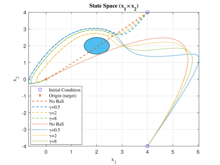
(a)

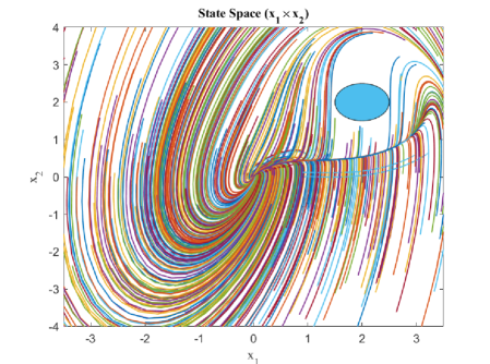
(b)

Figure 1: The top figure shows numerical simulations of the closed loop system starting from different initial conditions (small circles) with different $\gamma$s using the pole placement method to place the poles at $(-3,-5)$. The bottom figure shows a phase portrait of the closed loop system under the safety embedded linear control $u=-22.63x_{1}+7.14x_{2}+102.96z$ with $\gamma=1$.

It is worth noting that this is a linear control design for an inherently nonlinear control problem and thus limitations and difficulties of linear controls to stabilize nonlinear systems apply. One could use any nonlinear control technique to design a safely stabilizing control. In the next section, we leverage the infinite horizon optimal control in the process of designing an efficacious optimal safe control as optimal control is a well suited paradigm for such a problem and it facilitates the design of nonlinear controllers.

V Safety Embedded Optimal Control

Consider the infinite horizon optimal control problem of minimizing some cost functional subject to the dynamics (1) and the safety condition (2). This has been a sought-after problem recently [10, 11, 12] where CBFs are used to solve constrained optimal control problems. In these efforts, it can be seen how difficult the problem is and thus various complex techniques have been developed to solve the problem. Using the proposed BaS, this problem can be solved directly using well-known unconstrained optimal control methods. A systematic approach toward solving this problem is to seek an optimal feedback controller $u=K(\bar{x})$ that minimizes

$$V(x(0),u(t))=\frac{1}{2}\int_{0}^{\infty}Q(\bar{x})+u^{\rm{T}}Ru\;dt$$ (8)

where $Q:\mathbb{R}^{n+q}\rightarrow\mathbb{R}^{+}\ \forall x\neq 0$ is analytic and its Hessian is positive definite and $R\succ 0$, subject to (LABEL:new_system,_safety_augmented). By Theorem 3, if this optimal control problem is successfully solved, then both safety and stability requirements are met. For such an infinite horizon optimal control problem, a necessary and sufficient condition is that the well-known Hamilton-Jacobi-Belmman (HJB) equation is satisfied,

$$\text{HJB}:=\min_{u}\ V_{\bar{x}}^{*}\big{(}\bar{f}(\bar{x})+\bar{g}(\bar{x})u\big{)}+\frac{1}{2}u^{\rm{T}}Ru+\frac{1}{2}Q(\bar{x})=0$$ (9)

with a boundary condition $V^{*}(0)=0$ where $V^{*}$ is the optimal solution, a.k.a. the value function, and $V_{\bar{x}}^{*}=\frac{\partial V^{*}}{\partial\bar{x}}$.

Theorem 4.

Consider the optimal control problem (LABEL:new_system,_safety_augmented)-(8) with analytic $f(x),g(x)$ and $h(x)$ and suppose that the pair $\big{(}\frac{\partial f}{\partial x}(0),g(0)\big{)}$ is stabilizable, $Q$ is analytic with positive definite Hessian and $R\succ 0$. Then, there exists a unique analytic value function $V^{*}(\bar{x})$ satisfying the HJB equation (9), which yields an optimal safe feedback control

$$u^{*}_{safe}(\bar{x})=-R^{-1}\bar{g}(\bar{x})V^{*}_{\bar{x}}(\bar{x})$$ (10)

Moreover, $V^{*}(\bar{x})$ is a Lyapunov function and $u^{*}_{safe}$ renders the origin of the closed loop system $\bar{f}(\bar{x})+\bar{g}(\bar{x})u^{*}_{safe}(\bar{x})$ asymptotically stable. Therefore, the barrier state $z$ is bounded guaranteeing the generation of safe trajectories.

Proof.

As remarked earlier in the letter, the embedded system (LABEL:new_system,_safety_augmented) preserves the continuous differentiability and stabilizability properties of (1) and thus satisfies the analyticity and stabilizability assumptions in [13, 14, 15] hence guaranteeing the existence and uniqueness of the value function $V^{*}(\bar{x})$ and the corresponding optimal controller $u^{*}_{safe}(\bar{x})$ described in (10). Furthermore, the origin of the resulting closed loop system is asymptotically stable by Lyapunov stability theory [14, 16] and by Theorem 3, $u^{*}_{safe}(\bar{x})$ is safe which completes the proof. ∎

Various techniques have been proposed in the literature to approximate the solution to the HJB equation or the associated optimal control [17, 15, 18, 19, 20, 13, 14]. In the next section, we utilize these efforts to produce a power series solution of the value function and its gradient to produce the optimal safe control (10) for the optimal control problem (8). Specifically, we mainly utilize the recursive analytic solution proposed in [14] and the nonlinear quadratic regulator (NLQR) in [13].

VI Numerical Implementation and Examples

To demonstrate the efficacy of the presented technique to produce a safe and stabilizing control, we use a single BaS to enforce safety for a model of an inverted pendulum on a cart, and multiple barrier states for a multi-mobile robot navigation task where two point-robots are asked to go to intersecting targets while avoiding collision and avoiding some unsafe region.

VI-A Second Order Inverted Pendulum on a Cart

This system is an unstable version with a state dependent input matrix of the mechanical system with unity parameters used in [7] to show the applicability of the Control Lyapunov–Barrier Function (CLBF) approach. The system is given by

$$\begin{split}&\dot{x}_{1}=x_{2}\\ &\dot{x}_{2}=\sin(x_{1})-0.5(\tanh(10x_{2})+x_{2})+\cos(x_{1})u\end{split}$$

It is desired to avoid low velocities when the angle is half way through to stabilize the pendulum at the upright position to steer clear of the $90^{\text{o}}$ angle where the system loses controllability due to the $\cos(x_{1})$ term in the input matrix $g(x)$. That is, there are two symmetrical decoupled unsafe sets and therefore the safe set can be represented by two functions $h_{1}$ and $h_{2}$ such that $\mathcal{C}=\{x\in\mathcal{D}\ |\ (x_{1}-2)^{2}+x_{2}^{2}>1\ \cap\ (x_{1}+2)^{2}+x_{2}^{2}>1\}$. We pick the Carroll BF with $\gamma=5$ and use equation (5) with $z(0)=\beta(x(0))-\beta(0)$ to generate a single BaS. To generate the optimal safe controller, it is chosen to minimize the functional (8), with $R=1,\ Q=1x_{1}^{2}+50x_{2}^{2}+0.5z$. It is worth mentioning that this is an optimal control problem and thus different performances can be achieved using different cost functionals.

Fig. 2 shows numerical simulations for the closed-loop system under a $3^{\text{rd}}$ order nonlinear quadratic regulator (NLQR) [13], i.e. the approximated value function for the optimal control problem is of order four. Clearly, the proposed technique is powerful enough to generate a safe and asymptotically stable closed loop system safety is embedded in the stability of the overall system. It can be seen that there is a small cusp when the trajectories cross the $90^{\text{o}}$ angle which is a result of the lose of controllability when $\cos(90^{\text{o}})=0$. If low velocities were allowed at that specific region, that is if no barrier states are used, the closed loop system will go unstable.

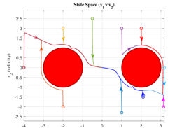
Figure 2: Numerical simulations of the closed-loop safety-critical system starting from different initial conditions (small circles). The goal is to stabilize the pendulum and avoid crossing the $90^{\text{o}}$ angle with low velocities, where the unsafe region is represented by the red circles. The proposed technique successfully generates safe trajectories and safely stabilizes the origin.

VI-B Multi Simple Mobile Robot Collision Avoidance

In this example, two simple mobile robots are asked to navigate their way toward prespecified targets. The robots are to avoid colliding as well as avoid an obstacle on their way. The robots dynamics are

$$\begin{split}\dot{x}_{i}=\begin{bmatrix}u_{i1}\\ u_{i2}\end{bmatrix},\dot{x}_{j}=\begin{bmatrix}u_{j1}\\ u_{j2}\end{bmatrix}\end{split}$$

To avoid collision, a BaS is featured through a barrier function that prevents the robots from getting too close to each other. We pick the maximum distance between the two robots to be $\delta=0.1$. Therefore, the associated safe set is $\{x_{i},x_{j}\in\mathcal{D}\ |\ ||x_{i}-x_{j}||^{2}>\delta^{2}\}$. Furthermore, we add an obstacle which is represented by a circle at $(0,0)$ with a radius of $0.25$. This calls for a BaS for each agent. Hence, the overall safe set for each agent is given by $\mathcal{C}=\{x_{k}\in\mathcal{D}\ |\ ||x_{i}-x_{j}||^{2}>\delta\;\text{and}\;x_{k1}^{2}+x_{k2}^{2}>0.25^{2},\;k=i,j\}$. For this example, we select the Log BF, $\beta_{l}=\log(\frac{1+h_{l}}{h_{l}})$ for $l=1,2,3$, to construct three barrier states, where the first represents the distance constraint between the two robots and the second and third barrier states represent the barriers needed to avoid the obstacle for agent $i$ and agent $j$ respectively. Using Table I, the barrier states are given by

$$\dot{z}_{l}=-\gamma_{l}\big{(}h_{l}(e^{z_{cl}}-1)^{2}-e^{z_{cl}}+1\big{)}-4\sinh^{2}(z_{cl}/2)h_{lx}u_{l}$$

with $z_{l}(0)=\beta_{l}(x(0))-\beta_{l}(0)$ for $l=1,2,3$ where $\gamma_{1}=15,\gamma_{2}=\gamma_{3}=0.5,z_{cl}=(z_{l}+c_{l}),c_{l}=\log(\frac{1+h_{l}(0)}{h_{l}(0)})$, $u_{1}=[u_{i}^{\rm{T}},u_{j}^{\rm{T}}]^{\rm{T}}$, $u_{2}=u_{i}$ and $u_{3}=u_{j}$. The cost functional (8) is selected such that $R=I_{4}$ and $Q=x_{i}^{\rm{T}}x_{i}+x_{j}^{\rm{T}}x_{j}+0.001z_{1}^{2}+0.5z_{2}^{2}+0.5z_{3}^{2}$. A $3^{\text{rd}}$ order NLQR is used in this example. As shown in Fig. 3, using the proposed technique, we are effectively able to send the two robots safely to the targeted positions while avoiding the obstacle as well as colliding with each other. The robots get very close to each other at sometime but never get too close, i.e. the distance between them is never less than or equal to $\delta$.

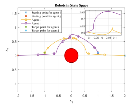
(a)

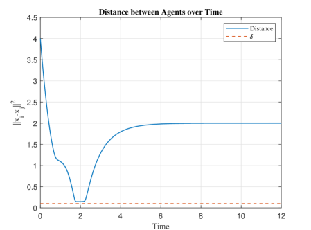
(b)

Figure 3: Two mobile robots starting from two opposite points sent to two opposite target points with an obstacle in-between. The two robots arrive at the desired locations safely. It can be seen that the two robots start by moving in a straight line toward their target points, which is the optimal behavior, but start to steer away to avoid the obstacle and then take some turns to avoid crossing the same point at the same time and to avoid getting too close (less than $\delta$ distance) to each other as shown in the bottom figure.

VII Conclusions and Future Works

A novel construction of safety embedded controls through the development of barrier states was presented. Through a proper conversion of barrier functions, barrier states were augmented to generate a nominal model which is safe if is asymptotically stable. Using barrier states, the constrained control problem was transformed to an unconstrained control problem, which makes the safety problem easier to be considered with various control techniques such as optimal control. Moreover, the BaS method is agnostic to the relative degree of the function describing the safe set with respect to the system unlike existing CBF based methods. Furthermore, there is no need to relax the stability requirement to guarantee safety as the two conditions are coupled and achieved simultaneously. The disadvantages of this approach include increasing the dimension of the model and adding nonlinearity to the model. The safety embedded model was used in constrained linear control and in the context of optimal control to generate safe stabilizing controllers. Simple linear controls and nonlinear quadratic controls were used to show the efficacy of the proposed method in various simulation examples.

Future work will include generalizations to nonlinear stochastic systems and applications to infinite and finite horizon stochastic optimal control as well as sampling-based model predictive control formulations. Another line of research includes generalizations of the proposed optimal control framework to min-max and $H_{\infty}$ optimal control problem formulations. Finally, incorporating uncertainty quantification methods into the augmented state space representation in (LABEL:new_system,_safety_augmented) is an active research.

References

- [1] Franco Blanchini “Set invariance in control” In Automatica 35.11 Elsevier, 1999, pp. 1747–1767
- [2] Stephen Prajna and Ali Jadbabaie “Safety verification of hybrid systems using barrier certificates” In International Workshop on Hybrid Systems: Computation and Control, 2004, pp. 477–492 Springer
- [3] Aaron D Ames et al. “Control barrier functions: Theory and applications” In 2019 18th European Control Conference (ECC), 2019, pp. 3420–3431 IEEE
- [4] Peter Wieland and Frank Allgöwer “Constructive safety using control barrier functions” In IFAC Proceedings Volumes 40.12 Elsevier, 2007, pp. 462–467
- [5] Muhammad Zakiyullah Romdlony and Bayu Jayawardhana “Uniting control Lyapunov and control barrier functions” In 53rd IEEE Conference on Decision and Control, 2014, pp. 2293–2298 IEEE
- [6] Aaron D Ames, Jessy W Grizzle and Paulo Tabuada “Control barrier function based quadratic programs with application to adaptive cruise control” In 53rd IEEE Conference on Decision and Control, 2014, pp. 6271–6278 IEEE
- [7] Muhammad Zakiyullah Romdlony and Bayu Jayawardhana “Stabilization with guaranteed safety using control Lyapunov–barrier function” In Automatica 66 Elsevier, 2016, pp. 39–47
- [8] Aaron D Ames, Xiangru Xu, Jessy W Grizzle and Paulo Tabuada “Control barrier function based quadratic programs for safety critical systems” In IEEE Transactions on Automatic Control 62.8 IEEE, 2016, pp. 3861–3876
- [9] Adrian G Wills and William P Heath “Barrier function based model predictive control” In Automatica 40.8 Elsevier, 2004, pp. 1415–1422
- [10] Yuxiao Chen, Mohamadreza Ahmadi and Aaron D Ames “Optimal safe controller synthesis: A density function approach” In 2020 American Control Conference (ACC), 2020, pp. 5407–5412 IEEE
- [11] Max H Cohen and Calin Belta “Approximate optimal control for safety-critical systems with control barrier functions” In 2020 59th IEEE Conference on Decision and Control (CDC), 2020, pp. 2062–2067 IEEE
- [12] Hassan Almubarak, Evangelos A Theodorou and Nader Sadegh “HJB Based Optimal Safe Control using Control Barrier Functions” In arXiv preprint arXiv:2106.15560, 2021
- [13] Hassan Almubarak, Nader Sadegh and David G. Taylor “Infinite horizon nonlinear quadratic cost regulator” In American Control Conference, 2019. Proceedings of the 2019, 2019 IEEE
- [14] Nader Sadegh and Hassan Almubarak “Recursive Analytic Solution of Nonlinear Optimal Regulators” In arXiv preprint arXiv:2006.15685, 2020
- [15] Dahlard L Lukes “Optimal regulation of nonlinear dynamical systems” In SIAM Journal on Control 7.1 SIAM, 1969, pp. 75–100
- [16] Hassan K Khalil “Nonlinear systems” Prentice Hall, 2002
- [17] EG Al’Brekht “On the optimal stabilization of nonlinear systems” In Journal of Applied Mathematics and Mechanics 25.5 Elsevier, 1961, pp. 1254–1266
- [18] Randal W Beard, George N Saridis and John T Wen “Approximate solutions to the time-invariant Hamilton–Jacobi–Bellman equation” In Journal of Optimization theory and Applications 96.3 Springer, 1998, pp. 589–626
- [19] Tayfun Cimen “State-dependent Riccati equation (SDRE) control: A survey” In IFAC Proceedings Volumes 41.2 Elsevier, 2008, pp. 3761–3775
- [20] Noboru Sakamoto and Arjan J Schaft “Analytical approximation methods for the stabilizing solution of the Hamilton–Jacobi equation” In IEEE Transactions on Automatic Control 53.10 IEEE, 2008, pp. 2335–2350