Towards Automatic Evaluation of Dialog Systems: A Model-Free Off-Policy Evaluation Approach

Abstract

Reliable automatic evaluation of dialogue systems under an interactive environment has long been overdue. An ideal environment for evaluating dialog systems, also known as the Turing test, needs to involve human interaction, which is usually not affordable for large scale experiments. Though researchers have attempted to use metrics (e.g., perplexity, BLEU) in language generation tasks or some model-based reinforcement learning methods (e.g., self-play evaluation) for automatic evaluation, these methods only show very weak correlation with the actual human evaluation in practice. To bridge such a gap, we propose a new framework named ENIGMA for estimating human evaluation scores based on recent advances of off-policy evaluation in reinforcement learning. ENIGMA only requires a handful of pre-collected experience data, and therefore does not involve human interaction with the target policy during the evaluation, making automatic evaluations feasible. More importantly, ENIGMA is model-free and agnostic to the behavior policies for collecting the experience data (see details in Section 2), which significantly alleviates the technical difficulties of modeling complex dialogue environments and human behaviors. Our experiments show that ENIGMA significantly outperforms existing methods in terms of correlation with human evaluation scores.

1 Introduction

Building dialog systems that can communicate unhindered with humans in natural language has been one of the most important goals of artificial general intelligence research since the 1950’s (Turing, 1950). One of the fundamental research bottlenecks for developing such dialog systems falls in evaluation, namely how to measure the performance of these systems in an automatic and scalable manner. Different from supervised natural language understanding tasks (e.g., text classification and machine translation), an ideal environment for evaluating dialog systems, also known as the Turing test, involves multi-turn human interaction (Turing, 1950; Liu et al., 2016; Ghandeharioun et al., 2019; See et al., 2019). While online platforms such as Amazon Mechanical Turk can provide human-based evaluation, they are often expensive and not scalable(Lowe et al., 2017).

Researchers have adopted language quality metrics for single-turn response generation given a fixed context (e.g., BLEU score and perplexity) to automatically evaluate dialog systems (DeVault et al., 2011; Xiang et al., 2014; Higashinaka et al., 2014; Gandhe and Traum, 2016; Lowe et al., 2017). However, these metrics only weakly correlate to human evaluation in practice (Liu et al., 2016; Ghandeharioun et al., 2019). One cause of such weak correlation is that language quality metrics rely on the exact match between generated text and ground-truth, which generally do not fully overlap. While certain embedding-based metrics have been developed to combat this lack of coverage (Mitchell and Lapata, 2008; Dziri et al., 2019), they are only post-hoc judgments based on static experience data, and does not necessarily reflect the dynamic quality of multi-turn interactive dialog well (Ghandeharioun et al., 2019). Moreover, evaluation of goal-oriented dialog systems should be based on how well dialog systems collect information from users and whether the goal is completed; language quality metrics are thus unable to meet these requirements.

To overcome the limitations of the aforementioned static evaluation methods, another line of work has proposed to model the interactive process of a conversation as a Markov decision process (MDP) (Möller et al., 2006; Li et al., 2016; Yu et al., 2016; Shah et al., 2018; Ghandeharioun et al., 2019; Jaques et al., 2019). Accordingly, automatic evaluation of dialog systems can be formulated as an off-policy evaluation (OPE) problem, where a human subject is the so-called “environment” in the reinforcement learning (RL) literature. For instance, Wei et al. (2018) propose a model-based approach for goal-oriented dialog systems. They first learn an environment/human model from the experience data consisting of human response, and then evaluate a dialog agent/policy by executing the policy within the learned environment. This procedure is known as “self-play evaluation”. Such a model-based approach requires accurate estimation of an environment/human when both input and output are in a combinatorially large space, i.e., the trained model needs to be able to mimic complex human behavior of generating meaningful sentences from huge vocabulary. Unfortunately, such a requirement is far beyond the current capability of model-based reinforcement learning algorithms. As a result, evaluations that rely on accurate modeling of the environment is often unreliable. A similar model-based approach is proposed (Ghandeharioun et al., 2019) to evaluate open-domain chit-chat dialog systems. In addition to modeling human behavior, they also model the reward function (for mimicking the complex mechanism behind human ratings) based on handcrafted features, which makes evaluation even more unreliable.

In this paper, we propose a general OPE framework named ENIGMA (EvaluatiNg dIaloG systeMs Automatically) for estimating human evaluation score (i.e., how a human would rate a dialog system). Different from the aforementioned model-based approaches, which rely on complex modeling of human behavior given combinatorially large vocabulary, ENIGMA takes advantage of recent advances in model-free OPE and avoids direct modeling of dynamic transitions and reward functions in a complex environment. Moreover, ENIGMA overcomes several limitations of existing OPE methods in order to evaluate dialog systems: (I) Existing OPE methods only apply to infinite or fixed horizon settings (where horizon length corresponds to number of turns in a conversation), while conversations, on the other hand, often have varying horizon lengths; (II) Existing OPE methods require experience data to sufficiently cover states and actions a target policy might visit. Due to limited experience data and the combinatorial nature of languages, such a requirement can hardly be satisfied in dialog evaluation; (III) Certain OPE methods rely on accurate estimation of the behavior policies used to collect the experience data. Unfortunately, such behavior policies are humans or complex dialog systems, and estimating their probabilistic model is essentially a challenging imitation learning problem.

To address (I), we propose a pseudo state padding method, which augments each conversation into infinitely many turns and yet preserves the original policy value; to address (II), we leverage pre-trained language models Devlin et al. (2018), which essentially transfer knowledge from open-domain data to alleviate the coverage issue; to address (III), we adopt a stationary distribution correction estimation approach Nachum et al. (2019a), which directly models the state-action density ratio between the experience data and the target policy Liu et al. (2018), and is therefore agnostic to the behavior policy. We summarize ENIGMA in comparison to existing works in Table 1.

We conduct thorough experiments on evaluating goal-oriented (AirDialog, Wei et al. (2018)) and chit-chat (ConvAI2, Dinan et al. (2020)) dialog systems to demonstrate the superiority of ENIGMA. Specifically, we follow the experimental settings similar to Ghandeharioun et al. (2019); See et al. (2019) (See details in Section 4), and show ENIGMA significantly outperforms the existing static evaluation and self-play evaluation methods in both domains.

The rest of this paper is organized as follows: Section 2 introduces the background of dialog systems and model-free OPE; Section 3 presents the ENIGMA framework for automatically evaluating dialog systems; Section 4 presents the experimental results and detailed analysis; more discussions on ENIGMA and related work are presented in Section 5.

Table 1: Comparison of existing works on Automatic Evaluation of Dialog Systems.

Method	Criterion	Dynamic	Model-Free	Behavior-Policy
BLEU, PPL	Language Quality	No	N/A	Human
Lowe et al. (2017)	Language Quality	No	N/A	Model & Human
Wei et al. (2018)	Task Completion	Yes	No	Human
Ghandeharioun et al. (2019)	Language Score	Yes	No	Model
ENIGMA	Both	Yes	Yes	Model

2 Background

$\bullet$ Dialog Generation as Markov Decision Process. A conversation is generated through interactions alternating between an agent $\pi$ (i.e., a dialog system) and an environment $\mathcal{E}$ (i.e., a human). We denote the dialog as $h=\{e_{0},a_{1},e_{1},...,a_{T}\}$, where $a_{i}$ and $e_{i}$ are sentences generated by $\pi$ and $\mathcal{E}$ respectively, and $T$ is the number of turns in the conversation. Dialog can be naturally described as a Markov decision process (MDP) (Puterman, 1995) $\mathcal{M}=\langle{\mathcal{S}},\mathcal{A},P,R,\mu_{0}\rangle$. Specifically, at the $t$-th turn, state $s_{t}\in{\mathcal{S}}$ captures the previous conversation history $s_{t}=\{e_{0},a_{1},e_{1},...,a_{t-1},e_{t-1}\}$. An action $a_{t}\in\mathcal{A}$ is an agent’s response given this context. Conversation can then be represented by the last state and action, i.e., $h=\{s_{T},a_{T}\}$. An agent $\pi$ is essentially a policy that maps ${\mathcal{S}}$ to $\mathcal{P}(\mathcal{A})$, where $\mathcal{P}(\cdot)$ denotes the set of probability measures over the action space. A transition kernel $P(\cdot|s_{t},a_{t})$ returns $s_{t+1}$ as the state at turn $t+1$, and an environment $\mathcal{E}$ generates a reward $r_{t}=R(s_{t},a_{t})\in[0,1]$. Note that $s_{t+1}$ essentially concatenates $s_{t}$ and $a_{t}$ with $e_{t}$, where $e_{t}$ is a response from the environment (i.e., human) at the $t$-th turn. The initial state $s_{1}=\{e_{0}\}$ is randomly sampled from some distribution $\mu_{0}$. An illustrative example of the dialog on booking a flight ticket is shown in Figure 1 (Wei et al., 2018).

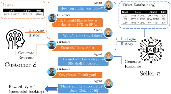
Figure 1: Dialog for booking a flight ticket (Airdialog).

Note that the reward $r_{t}=R(s_{t},a_{t})$ generated by the environment depends on the purpose of the dialog system: for open-domain chit-chat dialog, $R$ measures language quality; for goal-oriented agents, $R$ measures task completion scores. In particular, we follow the sparse reward setting, where each conversation is only evaluated at the ending state, i.e., $r_{t}=0$ for $t<T$ (Wei et al., 2018).

$\bullet$ Automatic Dialog Evaluation as Off-Policy Evaluation. Dialog evaluation can be naturally viewed as computing the expected reward of the above MDP defined as

$$\rho(\pi)=\mathbb{E}_{h\sim\mu_{0},\pi,\mathcal{E}}[R(s_{T},a_{T})],$$ (1)

where $h=\{s_{T},a_{T}\}$ is sampled from the initial distribution $\mu_{0}$ and the interaction between $\pi$ and $\mathcal{E}$. When the environment (i.e., human) is accessible, $\rho(\pi)$ can be directly estimated by interaction with the environment, which is known as on-policy evaluation (Sutton and Barto, 2018).

In dialog systems, however, interaction with human is expensive or prohibitive in practice, so human-free automatic evaluation is desired. Off-policy evaluation (OPE) (Precup, 2000) is an appealing choice when access to the environment is limited or unavailable. In particular, OPE can estimate $\rho(\pi)$ based solely on pre-collected tuples $\left\{\left(s,a,r,s^{\prime}\right)_{i}\right\}_{i=1}^{N}$ from behavior policies that are different from $\pi$.

OPE has been considered as one of the most fundamental problems in RL. A straightforward approach is to first directly learn an environment model ($R$ and $P$) from experience data and then estimate $\rho(\pi)$ by executing the policy within the learned environment. Such model-based OPE exactly corresponds to the so-called “self-play evaluation” in the dialog system literature (Wei et al., 2018; Ghandeharioun et al., 2019). Unfortunately, it is notoriously difficult to specify a proper model for highly complicated environments such as a dialog environment (i.e., a human), where the state and action spaces are combinatorially large due to huge vocabulary size and complex transitions. As a result, the estimation error of the environment accumulates as interaction proceeds, and model-based self-play evaluation of dialog systems often becomes unreliable (Voloshin et al., 2019).

To address the challenge above, many model-free OPE methods that avoid direct modeling of the environment have been proposed. Model-free OPE can be categorized into behavior-aware and behavior-agnostic methods. Specifically, behavior-aware methods rely on either knowing or accurately estimating the probabilistic model of behavior policies used for collecting the experience data (e.g., inverse propensity scoring, Horvitz and Thompson (1952)). Unfortunately, behavior policies are often unknown in practice. Estimating their probabilistic models is also quite challenging, as it requires modeling human behaviors or complex dialog systems. Behavior-agnostic methods, on the other hand, do not require explicit knowledge or direct modeling of behavior policies, and are therefore more favorable when experience data is collected by multiple (potentially unknown) behavior policies.

Unfortunately, most of the existing model-free behavior-agnostic OPE methods focus on either infinite-horizon (Nachum et al., 2019a; Zhang et al., 2020b; Yang et al., 2020) or fixed-horizon settings (Yin and Wang, 2020; Duan and Wang, 2020), and cannot be applied to evaluating dialog systems whose horizon (number of turns) vary between conversations. While LSTDQ (Lagoudakis and Parr, 2003) can be adopted to handle varying horizons, it has been shown to not work well under the sparse reward setting Lagoudakis and Parr (2003); Mataric (1994).

3 ENIGMA

We present the ENIGMA framework for automatically evaluating dialog systems using experience data. In particular, ENIGMA is model-free and agnostic to behavior policies for generating the experience data. ENIGMA has three major ingredients: (1) pseudo-state padding for converting a dialog into an infinite-horizon MDP, (2) distribution-correction estimation (DICE, Nachum et al. (2019a)) with post-normalization for estimating the value of the target policy based on experience data, and (3) function approximation and representation learning with pre-trained language models.

3.1 Pseudo-State Padding

As mentioned in Section 2, existing model-free behavior-agnostic OPE methods cannot handle varying horizon lengths in conversations under the sparse reward setting. To address this issue, we design a special padding scheme, so that the policy value can be estimated by OPE methods from the resulting padded MDP. We first pad conversation sequences with pseudo states, which leads to a padded MDP with a fixed horizon length $T_{\rm max}$. We then convert such a fixed horizon MDP into infinite horizon by augmentation, i.e., we repeatedly concatenate the ending state of the fixed horizon MDP to its initial state.

More specifically, as illustrated in Figures 2, the policy takes a deterministic action at all pseudo states, i.e., $\pi(a={\rm NextPad}|s={\rm Pad}_{k})=1$. The transition kernel of the new process can be defined as

This new process is still a valid MDP, as its transition kernel satisfies the Markov property. For notational simplicity, we refer to such an augmented MDP with infinite horizon as “the augmented MDP”.

Accordingly, the policy value of $\pi$ for the augmented MDP can be defined as

$$\rho_{A}(\pi)\textstyle=\lim_{N\rightarrow\infty} {\mathbb{E}}_{(h_{1},h_{2},...,h_{N})\sim\mu_{0},\pi,\mathcal{E}}\textstyle[\frac{1}{NT_{\rm max}}\sum_{i=1}^{N}\sum_{t=1}^{T_{\rm max}}R(s_{t}^{(i)},a_{t}^{(i)})],$$ (2)

where $h_{i}$’s are padded conversations sampled from interactions between $\pi$ and $\mathcal{E}$. Since there is only one non-zero reward for every $T_{\rm max}$ steps, rewards in the augmented MDP are also sparse.

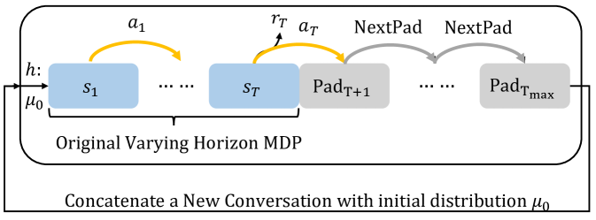
Figure 2: Augmented MDP with Infinite Horizon.

We justify such a padding scheme in the following theorem showing that the augmented MDP has a unique stationary distribution, and guarantees any policy $\pi$ to have a finite policy value. Moreover, the policy value of $\pi$ under the augmented MDP is proportional to its counterpart under the original MDP without augmentation. Due to space limit, we defer the proof to Appendix A.1.

Theorem 1.

The augmented MDP with infinite horizon satisfies the following properties: $\bullet$ It has a unique stationary state-action visitation distribution $d^{\pi}(s,a)$;

$\bullet$ For the state-action pair $(s_{t},a_{t})$ in a conversation $h$ with padded pseudo states, we have

$$d^{\pi}(s_{t},a_{t})= \textstyle\frac{1}{T_{\rm max}}\sum_{\{(s_{k},a_{k})\}_{k=1}^{t-1}}[\mu_{0}(s_{1})\pi(a_{1}|s_{1})$$

$$P(s_{2}|a_{1},s_{1})\cdots P(s_{t}|a_{t-1},s_{t-1})\pi(a_{t}|s_{t})],$$ (3)

where $\{(s_{k},a_{k})\}_{k=1}^{t-1}$ are the state-action pairs in the same conversation as $(s_{t},a_{t})$;

$\bullet$ The policy value can be computed by sampling from $d^{\pi}(s,a)$, and we have

$$\rho_{A}(\pi)={\mathbb{E}}_{(s,a)\sim d^{\pi}(s,a)}[R(s,a)]=\rho(\pi)/T_{\rm max}.$$ (4)

Remark 1.

Some OPE methods, e.g., LSTDQ Lagoudakis and Parr (2003), can handle fixed horizons, therefore only applying the fixed-horizon padding would suffice. DICE estimators (Nachum et al., 2019a), on the other hand, can only handle infinite horizons, therefore the infinite-horizon augmentation is necessary.

Remark 2.

Note that in practice, we do not actually need to concatenate infinitely many conversations for computing $\rho_{A}(\pi)$. As suggested by (4), $\rho_{A}(\pi)$ can be computed based on $d^{\pi}(s_{t},a_{t})$ defined in (3), which is the product of only finite terms.

3.2 Model-Free Behavior-Agnostic DICE Estimator

With the proposed augmentation, we obtain an infinite horizon MDP from which the policy value of the original MDP can be recovered. We then apply DICE (Nachum et al., 2019a; Yang et al., 2020) to estimate $\rho_{A}(\pi)$ based on pre-collected experience data $\mathcal{D}=\left\{\left(s,a,r,s^{\prime}\right)_{i}\right\}_{i=1}^{N}$ without interacting with $\mathcal{E}$ (i.e., a human), where $(s,a)\sim d^{\mathcal{D}}$ are samples from some unknown distribution $d^{\mathcal{D}}$. We slightly abuse the notations and use $(s,a,r,s^{\prime})\sim d^{\mathcal{D}}$ as a shorthand for $(s,a)\sim d^{\mathcal{D}},r=R(s,a),s^{\prime}\sim P(\cdot|s,a)$, which simulates sampling form the dataset $\mathcal{D}$.

DICE is a model-free policy evaluation method (without explicitly modeling $\mathcal{E}$) and does not require knowledge of behavior policies for generating the experience data, which provides a more reliable estimation of $\rho_{A}(\pi)$ than other OPE methods. Specifically, DICE decomposes $\rho_{A}(\pi)$ into:

$$\rho_{A}(\pi)=\mathbb{E}_{(s,a,r)\sim d^{\mathcal{D}}}[\zeta(s,a)r],$$ (5)

where $\zeta(s,a):=d^{\pi}(s,a)/d^{\mathcal{D}}(s,a)$ is the distribution correction ratio. Then DICE estimates $\zeta$ by solving the following regularized minimax optimization problem:

$$\max_{\zeta\geq 0}\min_{\nu,\lambda} L_{D}(\zeta,\nu,\lambda)=\mathbb{E}_{(s,a,r,s^{\prime})\sim d^{\mathcal{D}},a^{\prime}\sim\pi(s^{\prime})}[\zeta(s,a)$$

$$\cdot(\nu(s^{\prime},a^{\prime})-\nu(s,a))]+\mathbb{E}_{(s,a)\sim d^{\mathcal{D}}}[\lambda(\zeta(s,a)$$

$$-1)]-\alpha_{\zeta}\cdot\mathbb{E}_{(s,a)\sim d^{\mathcal{D}}}[f(\zeta(s,a))].$$ (6)

where $\nu(s,a)$’s are auxiliary variables, $f$ is a convex regularizer (e.g., $f(x)=x^{2}$), and $\alpha_{\zeta}$ is a tuning parameter. Due to the space limit, we omit the details of deriving the DICE estimator. Please refer to Yang et al. (2020) for more technical details.

$\bullet$ Post-Normalization. Note that (3.2) handles the constraint $\mathbb{E}_{(s,a)\sim d^{\mathcal{D}}}\zeta(s,a)=1$ by Lagrange multipliers $\lambda$, which cannot guarantee that the constraint is exactly satisfied when solving (3.2) using alternating SGD-type algorithms (Dai et al., 2017; Chen et al., 2018). To address this issue, we propose a post-normalization step that explicitly enforces the constraint:

$$\textstyle\rho_{n}(\pi)=\sum_{(s,a,r)\sim d^{\mathcal{D}}}{\zeta}(s,a)r\Big{/}\sum_{(s,a)\sim d^{\mathcal{D}}}{\zeta}(s,a).$$ (7)

As we will see in our experiments in Section 4, the post-normalization step is crucial for DICE to attain good estimation accuracy in practice; without the post-normalization, we observe potential divergence in terms of policy value estimation.

$\bullet$ Why do we prefer DICE? Deep Q-learning and its variants are another popular model-free and behavior-agnostic approach to off-policy evaluation. However, due to the sparse rewards in dialogs, fitting the state-action value function (i.e., the $Q$-function) in deep Q-learning is notoriously difficult (Mataric, 1994). We observe in Section 4 that deep Q-learning is computationally unstable.

In contrast, DICE only needs to estimate the density correction ratio $\zeta$, which is decoupled from the rewards associated with the policy value as shown from (3.2). This significantly alleviates the computational challenge incurred by sparse rewards. Moreover, DICE also applies the post-normalization, additional regularization (i.e., $\mathbb{E}_{(s,a)\sim d^{\mathcal{D}}}[f(\zeta(s,a))]$), and constraints on $\zeta$ (i.e., $\zeta\geq 0$ and $\mathbb{E}_{(s,a)\sim d^{\mathcal{D}}}[\zeta(s,a)]=1$), all of which further stabilize training. These features allow DICE achieve better estimation performance than deep Q-learning in dialog systems evaluation.

Recent progresses in OPE based on density ratio estimation are remarkable (Liu et al., 2018; Nachum et al., 2019a; Xie et al., 2019; Uehara et al., 2019), however, there exists a statistical limit in off-policy evaluation. Specifically, the Cramer-Rao lower bound of the MSE has been established in Jiang and Li (2016), which is proportional to the square of the density ratio. This implies that we can only obtain accurate estimation of policy value only if the ratio $\zeta$ is not too large. While the ratio-based minimax algorithms should have achieved the asymptotic lower bound (Kallus and Uehara, 2019; Yin and Wang, 2020), even better estimation results can be obtained when behavior and target policies are more similar. We thus introduce an experience data collection protocol in Section 4.1 which satisfies the bounded ratio requirement and ensures the success of OPE methods.

3.3 Function Approximation with RoBERTa

Despite the apparent advantages of DICE estimators, directly training DICE from scratch will fall short due to the bounded ratio requirement being quickly broken in the large combinatorial state-action space in dialog.

We alleviate this issue by learning reliable representations from an enormous amount of pre-collected data. We resort to the domain transfer learning technique, also known as language model pre-trained and fine-tuning Devlin et al. (2018). For example, RoBERTa(Liu et al., 2019) is an extremely large bidirectional transformer model (Vaswani et al., 2017) pre-trained using huge amounts of open-domain text data in a self-supervised/unsupervised manner. RoBERTa is particularly attractive to the dialog evaluation task due to the following merits: (1) the pre-training process does not require any labelled data; (2) the pre-trained models are publicly available; (3) the massive model sizes (usually with hundreds of millions or billions of parameters) allow these models to effectively capture rich semantic and syntactic information of natural language (rather than enumerating the original combinatorial language space).

To transfer the knowledge from the pre-trained RoBERTa model to dialog evaluation, we parameterize $\zeta$ and $\nu$ as follows: We keep the pre-trained RoBERTa encoder layer and replace the original mask language modeling head by a two-layer fully connected network with a scalar output. For simplicity, we denote the corresponding parametric forms of $\zeta$ and $\nu$ as RoBERTa-$\zeta$ and RoBERTa-$\nu$, respectively. Note that we only need RoBERTa-$\zeta$ and RoBERTa-$\nu$ to share the same encoder, as illustrated in Figure 3. We then use RoBERTa-$\zeta$ and RoBERTa-$\nu$ as the initial solution to solve (3.2), which is also known as the fine-tuning step (Devlin et al., 2018; Liu et al., 2019).

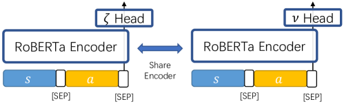
Figure 3: Function Approximation with RoBERTa.

With a properly designed mask, the self-attention mechanism in the bi-direction transformer architecture allows us to efficiently compute $\zeta(s,a)$ and $\nu(s,a)$ for all state-action pairs in the same dialog simultaneously. Due to the space limit, we defer the mask design details to Appendix A.2.

3.4 Summary

We summarize ENIGMA using SGD with batch-size 1 in Algorithm 1. We defer the details of ENIGMA with mini-batch SGD to Appendix A.3 (Algorithm 2).

Algorithm 1 ENIGMA

1:Experience conversations $\mathcal{D}=\{(h_{i}=\{e^{(i)}_{0},a^{(i)}_{1},e^{(i)}_{1},...,a^{(i)}_{T_{i}}\},r^{(i)})\}_{i=1}^{N}$, Target Policy $\pi$, Padding Length $T_{\rm max}$, Regularization function $f$, DICE hyper-parameters $\alpha_{\zeta}$, $\alpha_{R}$

2:Performance Estimation $\widehat{\rho}_{n}(\pi)$

3:$\zeta=\{$RoBERTa-$\zeta,[\zeta_{{\rm pad},t}]_{t=1}^{T_{\rm max}}\}$, $\nu=\{$RoBERTa-$\nu,[\nu_{{\rm pad},t}]]_{t=1}^{T_{\rm max}}\}$, $\lambda$

4:while  Sample $({h},r)$ in $\mathcal{D}$  do

5:     $\zeta_{0}=\zeta_{{\rm pad},T_{\rm max}}$,   $\nu_{0}=\nu^{\prime}_{0}=\nu_{{\rm pad},T_{\rm max}}$

6:     for $t$ in $1,\cdots,T$ do

7:         $\zeta_{t}=$ RoBERTa-$\zeta(e_{0},a_{1},...,e_{t-1},a_{t})$

8:         $\nu_{t}=$ RoBERTa-$\nu(e_{0},a_{1},...,e_{t-1},a_{t})$

9:         $\widetilde{a}_{t}\sim\pi(e_{0},a_{1},...,e_{t-1})$

10:         $\nu^{\prime}_{t}=$ RoBERTa-$\nu(e_{0},a_{1},...,e_{t-1},{\color[rgb]{1,0,0}\widetilde{a}_{t}})$

11:     end for

12:     for $t$ in $T+1,\cdots,T_{\rm max}$ do

13:         $\zeta_{t}=\zeta_{{\rm pad},t}$,   $\nu_{t}=\nu^{\prime}_{t}=\nu_{{\rm pad},t}$

14:     end for

15:     $L_{D}(\zeta,\nu,\lambda)=\frac{1}{T_{\rm max}}[\sum_{t=0}^{T_{\rm max}-1}[\zeta_{t}(\nu^{\prime}_{t+1}-\nu_{t})+\lambda(\zeta_{t}-1)-\alpha_{\zeta}f(\zeta_{t})]]$

16:     SGD update based on $\frac{\partial L_{D}}{\partial\nu}$,$\frac{\partial L_{D}}{\partial\lambda}$,$\frac{\partial-L_{D}}{\partial\zeta}$.

17:end while

18:for  $({h}_{i},r^{(i)})$ in $\mathcal{D}$ do

19:     $\zeta_{i}=$ RoBERTa-$\zeta({h}_{i})$

20:end for

21:Return $\widehat{\rho}_{n}(\pi)=\sum_{i}\zeta_{i}r^{(i)}\big{/}\sum_{i}\zeta_{i}$

4 Experiments

We empirically evaluate ENIGMA on two dialog datasets: AirDialog (Wei et al., 2018) for goal-oriented tasks and ConvAI2 (Dinan et al., 2020) for open-domain chit-chat respectively. See details of experimental setup in Appendix B.

4.1 Policy Training Data and Experience Data

As mentioned in Section 3.2, there exists an information theoretic limit for all off-policy evaluation methods: no method can perform well when the state-action density ratio between the target and behavior policy is too large. To avoid such a circumstance, we need to ensure that the experience data collected by a behavior policy do not deviate too much from data induced by the target policy. Unfortunately, both datasets used in our experiments do not satisfy such a requirement. AirDialog, for example, consists of dialog between humans, which are near-perfect golden samples as human agents almost always successfully book tickets for customers. Dialog system agents, on the other hand, have many failure modes (i.e., the target policy/agent does not book the correct ticket for a human customer). Hence, directly using human dialog as the behavior data to evaluate dialog agents is subject to limitations.

In order to properly evaluate an imperfect target policy in the presence of the information theoretic limit, we refer to Lowe et al. (2017); Ghandeharioun et al. (2019); See et al. (2019), and collect experience data using behavior policies similar to the target policy. To avoid confusion, we call data collected by the behavior policy “experience data” and data used to train an agent “policy training data”. More details are elaborated below for each dataset.

It is worth noting that existing work on dialog systems evaluation also enforces similar requirements. For example, Lowe et al. (2017) show higher Pearson correlation coefficient ($0.37$) between automatic metrics and human ratings when behavior policies contain the target policy. When the target policy is excluded from behavior policies, however, the correlation is only $0.13$, even lower than the meaningless correlation between dialog lengths and human ratings ($0.27$). Another example is Ghandeharioun et al. (2019), where the studied agents are similar to each other in their hierarchical architectures, hyperparameters, and training data.

We compare the experience data used in this paper with existing works in Table 2.

Table 2: Number of Dialogues/Agents in Experience Data. ^†: 4,104 dialog turns and the number of dialogs is not avaliable.

Experience Data	Agents	Dialogs
Lowe et al. (2017)	4	N/A †
Ghandeharioun et al. (2019)	12	512
Ours-Airdialog	24	2400
Ours-ConvAI2	29	2616

4.2 Goal-Oriented Systems

We first test ENIGMA  for evaluating goal-oriented dialog systems on a flight ticket booking task.

$\bullet$ Policy Training Data. We use the AirDialog dataset for policy training Wei et al. (2018). It contains 402,038 pieces of dialog from human sellers and human customers collaborating on buying flight tickets. We use different proportions of the dataset and different hyperparameters to train 24 seller agents using behavior cloning (See Appendix C for details) .

$\bullet$ Experience Data. We invite 20 people to evaluate the 24 seller agents. Specifically, each of the 20 human customers interacts with a seller agent 5 times to generate 100 pieces of dialog, and gives each piece an evaluation score between 0 and 1. The final score an agent receives is the average of the 100 scores. We consider three types of scores: flight score, status score, and overall reward used in Wei et al. (2018).

Table 3: The correlation between two metrics. Each column is a task completion score obtained by interacting human customers (“Selected Agents” denotes only evaluating agents with reasonably good performance).

Setting	Method	Pearson Correlation				Spearman’s Rank Correlation
		Flight Score	Status Score	Reward	Average	Flight Score	Status Score	Reward	Average
	BLEU	0.1450	-0.1907	-0.0709	-0.0389	0.0370	-0.1453	-0.1472	-0.0852
All	PPL	-0.1598	0.1325	0.0195	-0.0026	-0.1817	0.0090	-0.0039	-0.0649
Agents	SPE	0.6450	0.7926	0.7482	0.7286	0.3539	0.8004	0.7400	0.6314
	ENIGMA	0.9255	0.9854	0.9672	0.9593	0.8948	0.9839	0.9435	0.9407
	BLEU	-0.0621	-0.1442	0.2944	0.0294	-0.1273	-0.2208	0.1793	-0.1758
Selected	PPL	-0.0197	-0.1775	0.0460	-0.0504	-0.1146	-0.4652	-0.0404	-0.2067
Agents	SPE	0.0970	0.5203	0.4777	0.3650	0.1368	0.5304	0.4943	0.3872
	ENIGMA	0.8640	0.9031	0.8952	0.8874	0.8496	0.9414	0.8782	0.8686

We evaluate ENIGMA, BLEU/PPL (Papineni et al., 2002) and Self-Play Evaluation (SPE) based on the correlation between estimated reward and true reward. The results are summarized in Table 3. ENIGMA uses the experience data of the other 23 agents to evaluate each agent (i.e., leave-one-bot-out). Note that SPE (Wei et al., 2018) needs to train a customer agent in addition to the seller agent being evaluated. For a fair comparison, we train the SPE customer agent on both experience data and policy training data (See Appendix C for details). Our empirical observations are as follows:

$\bullet$ ENIGMA vs. BLEU/PPL. ENIGMA significantly outperforms BLEU/PPL. As mentioned earlier, BLEU and PPL are well-known metrics for evaluating language quality. For goal-oriented systems whose goal is to complete a specific task, however, BLEU and PPL scores show little correlation with task completion scores.

$\bullet$ ENIGMA vs. SPE. ENIGMA significantly outperforms SPE. To better understand their performance, we also present the regression plots between estimated and true rewards in Figure 4. Both ENIGMA and SPE can easily identify agents with extremely poor rewards. However, for selected good agents whose flight score, status score, and overall reward are better than $0.5$, $0.7$, and $0.65$ respectively, SPE performs worse than ENIGMA by a much larger margin (especially for flight score). Additional regression plots are shown in Appendix D.1.

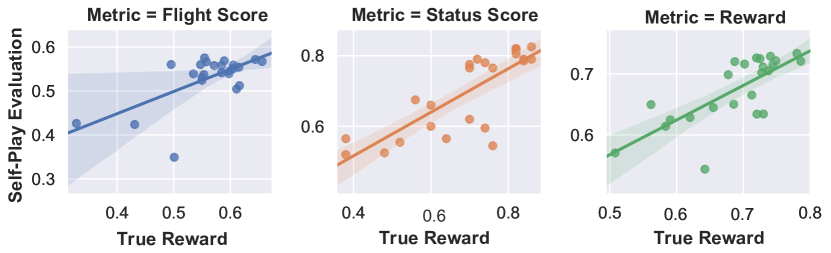
(a) SPE vs. Human Evaluation

(b) ENIGMA vs. Human Evaluation

Figure 4: Regression Plots. The x-axis is the average reward obtained by chatting with human. The y-axis is the reward estimated by SPE / ENIGMA. Different colors denote different types of rewards (flight score, status score, and overall reward). The solid line is obtained by linear regression and the shaded region indicates $95\%$ confidence interval.

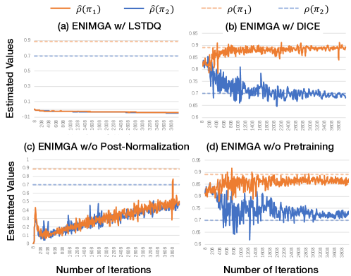
Figure 5: Value estimation using different methods for two target agents ($\pi_{1}$ and $\pi_{2}$) vs. # of iterations. Dotted lines denote the true rewards.

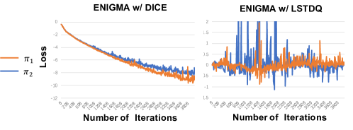
Figure 6: Training Objectives vs. Number of Iterations for two target agents.

$\bullet$ Ablation Study. We select 2 out of the 24 agents to illustrate the importance of each component in ENIGMA.

$\star$ DICE vs. LSTDQ. Figure 5(a) and Figure 5(b) show the estimated values of LSTDQ (only fitting the $Q$-function) and DICE respectively: estimates of LSTDQ are stuck at 0 whereas estimates of DICE approach the true rewards (dotted lines) as training progresses. Figure 6 additionally shows that the training objectives of LSTDQ oscillates as DICE stably converges.

$\star$ Post-normalization. Figure 5(c) shows the performance of ENIGMA without post-normalization: The estimated values fail to approach the true rewards.

$\star$ Pretrained Encoder. Figure 5(d) shows the performance of ENIGMA without the pretrained encoder: The estimated values can approach the true rewards, but are less stable and less accurate than the counterpart with the pretrained encoder.

(a) SPE vs. Human Evaluation

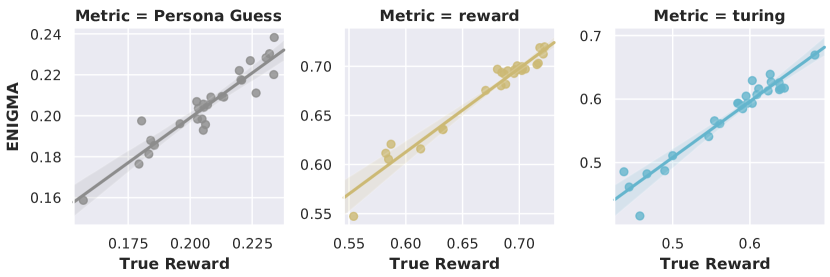
(b) ENIGMA vs. Human Evaluation

Figure 7: Regression Plots. Only three metrics are presented. Please refer to Appendix D.3 for all plots.

4.3 Open-Domain Chit-chat Systems

We now test ENIGMA  for evaluating open-domain chit-chat dialog systems.

$\bullet$ Policy Training Data. We use 29 pre-trained agents provided by See et al. (2019). These agents are trained using behavior cloning on the ConvAI2 dataset Zhang et al. (2018); Dinan et al. (2020). The dataset contains 8,939 pieces of dialog, where participants are instructed to chat naturally using given personas.

$\bullet$ Experience Data. We use the experience dataset provided by See et al. (2019). The dataset contains 3,316 agent-human evaluation logs and 10 different language quality metrics for each log.

Table 4: The correlation between automatic metrics and language score obtained by interacting with human. We only present the average/min/max correlations to all 10 different language metrics in this table. For detailed numbers, please refer to Appendix D.3, Figure 25.

Method	Experience Data	Pearson Correlation			Spearman’s Rank Correlation
		Average	Min	Max	Average	Min	Max
Best of 8 HCDFs	Human-Human	0.6045	0.4468	0.9352	0.3384	0.1724	0.7526
8 HCDFs + Regression	Human-Human	0.5387	-0.0348	0.7519	0.4740	0.2784	0.7880
BLEU	Human-Human	0.4127	0.0671	0.6785	0.2965	0.0482	0.7236
BLEURT	Human-Human	0.4513	0.1557	0.6572	0.4389	0.0055	0.6864
BERTscore F-1	Human-Human	0.5365	0.0609	0.8385	0.5293	0.2852	0.7044
SPE	Human-Model	0.5907	0.0962	0.8820	0.4350	0.1363	0.6405
SPE	Human-Model (Challenging)	0.3559	-0.1679	0.6900	0.1429	-0.0777	0.3216
ENIGMA	Human-Model	0.9666	0.9415	0.9792	0.9167	0.8717	0.9485
ENIGMA	Human-Model (50% data)	0.9126	0.8506	0.9585	0.7790	0.6651	0.8647
ENIGMA	Human-Model (10% data)	0.7327	0.4544	0.9266	0.5214	0.3651	0.6492
ENIGMA	Human-Model (Challenging)	0.6505	0.5394	0.7762	0.5190	0.3168	0.6672

We follow the setups from Section 4.2 to evaluate, ENIGMA, SPE, BLEU, BLEURT (Sellam et al., 2020), BERTscore (Zhang et al., 2019), and 8 Hand-Crafted Dialog Features (HCDFs) based on Pearson and Spearman’s rank correlations between the estimated rewards and the true rewards. Here the true rewards are human evaluation scores under 10 different language quality metrics. More details of HCDFs and language quality metrics can be found in See et al. (2019). The average, minimum and maximum of the 10 correlations (under different language quality metrics) of each method are summarized in Table 4. Moreover, we also consider using 8 HCDFs to fit the true rewards using linear regression, and the results are also included in Table 4.

Note that since we are considering a chit-chat dialog system, SPE does not train an additional agent but asks two identical target agents to chat with each other. However, SPE needs to train an additional model to predict the reward of each dialog. Specifically, we fine-tune the pre-trained RoBERTa encoder with an output layer over the experience data (an additional sigmoid function is applied to ensure an output between 0 and 1). For automatic evaluation of each agent using ENIGMA, we use the experience data of the other 28 agents (i.e., leave-one-bot-out).

$\bullet$ ENIGMA vs. SPE/BLEU/BLEURT/BERTscore/HCDFs. ENIGMA significantly outperforms SPE, BLEU, BLEURT, BERTscore and HCDFs in both Pearson and Spearman’s rank correlations. Moreover, we compare the correlations between estimated rewards and human evaluation scores under each language quality metric. Due to space limit, we only show the plots of ENIGMA and SPE under 3 out of 10 language quality metrics in Figure 7. Additional plots and detailed results can be found in Appendix D.3. We see that ENIGMA outperforms SPE and HCDFs under all language equality metrics.

$\bullet$ Sample Efficiency of ENIGMA. To demonstrate that ENIGMA is sample efficient, we test ENIGMA on randomly sub-sampled (10% and 50%) experience data. We found that even using only 10% of the experience data, ENIGMA still outperforms SPE and HCDFs.

$\bullet$ Evaluation under Challenging Experience Data. To make the evaluation more challenging, we further test ENIGMA by excluding the experience data obtained by the behavior policies similar to the target policy (see more details in Appendix D.3). We see that even with such challenging experience data, ENIGMA still outperforms SPE with trained on full data and HCDFs under almost all language quality metrics.

5 Discussions

Existing research on automatic evaluation of dialog systems can be categorized into static vs. dynamic evaluation. Most of existing research falls into static evaluation with a focus on language quality of single-turn response or on task-completion given fixed dialog, while few literature emphasizes dynamic properties of an interactive environment. Different from static evaluation, dynamic evaluation considers the sequential interaction between a human and an agent, and thus it is more challenging.

We note that in both static and dynamic evaluations, algorithms rely on the assumption of sufficient data coverage (explicitly or implicitly) to ensure reliable evaluation. For example, in static evaluation, BLEU score requires all reasonably good responses to be exactly covered by the experience data. More recently, Lowe et al. (2017) show that their method only works when the behavior policies include the target policy. Dynamic evaluation also assumes the sufficient coverage. We emphasize that it is the information-theoretic limit of all OPE methods (Jiang and Li, 2016), which requires the experience data to cover sufficient target policy behaviors to ensure accurate estimation. Therefore, we suggest the broader research community to release human-model interaction evaluation data to further promote research in automatic dialog systems evaluation.

6 Conclusion

We develop a model-free OPE framework, ENIGMA, for evaluating dialog systems using experience data. By adopting the current state-of-the-art OPE method in reinforcement learning, we tackle several challenges in modeling dialog systems. Different from existing single-turn language quality metrics and model-based reinforcement learning methods, ENIGMA naturally takes into consideration the interactive and dynamic nature of conversations, while avoiding the difficulty of modeling complex human conversational behaviors. Our thorough experimental results demonstrate that ENIGMA significantly outperforms existing methods in terms of correlation with human evaluation scores. One potential future direction is to extend ENIGMA from off-policy evaluation to off-policy improvement, which aims to learn a dialog system based on experience data (Nachum et al., 2019b; Kallus and Uehara, 2020).

Appendix A ENIGMA

A.1 Supporting Theorem

Theorem 1.

The augmented MDP with infinite horizon satisfies the following properties:

• It has a unique stationary state-action visitation distribution $d^{\pi}(s,a)$;

• For the station-action pair $(s_{t},a_{t})$ in a conversation $h$ with padded pseudo states, we have

  $$d^{\pi}(s_{t},a_{t})=\frac{1}{T_{\rm max}}\sum_{\{(s_{k},a_{k})\}_{k=1}^{t-1}}[\mu_{0}(s_{1})\pi(a_{1}|s_{1})P(s_{2}|a_{1},s_{1})\cdots P(s_{t}|a_{t-1},s_{t-1})\pi(a_{t}|s_{t})],$$ (8)

  where $\{(s_{k},a_{k})\}_{k=1}^{t-1}$ are the state-action pairs in the same conversation as $(s_{t},a_{t})$;

• The policy value can be computed by sampling from $d^{\pi}(s,a)$, and we have

  $$\rho_{A}(\pi)={\mathbb{E}}_{(s,a)\sim d^{\pi}(s,a)}[R(s,a)]=\rho(\pi)/T_{\rm max}.$$ (9)

Proof.

First, we prove that the augmented MDP has a unique stationary state-action visitation distribution shown in (8).

As the augmented MDP is periodic with period $T_{\rm max}$, the uniqueness and stationary distribution can not be immediately obtained by ergodicity of the MDP (the first two points of the Theorem).

To obtain the stationary state-action visitation distribution, we essentially need to solve the following equations:

$$d^{\pi}(s,a)=\sum_{(s^{\prime},a^{\prime})}d^{\pi}(s^{\prime},a^{\prime})P(s|s^{\prime},a^{\prime})\pi(a|s),~{}~{}{\rm for~{}all}~{}~{}(s,a)$$ (10)

with $d^{\pi}(s,a)$ is a probability measure on the state-action space, i.e., $\sum_{(s,a)}d^{\pi}(s,a)=1$.

We first group the state-action pairs by their dialog turns $t$. More specifically, we define ${\mathcal{S}}_{t}:=\{s_{t}:s_{t}{\rm~{}contains~{}}t{\rm~{}dialog~{}turns}\}$, $\mathcal{A}_{t}:=\{a_{t}:a_{t}{\rm~{}is~{}the~{}response~{}at~{}the~{}}t{\rm-th~{}dialog~{}turn}\}$ and $\mathcal{Q}_{t}={\mathcal{S}}_{t}\times\mathcal{A}_{t}$. We have the state space is the direct sum of state groups ${\mathcal{S}}_{0}\oplus{\mathcal{S}}_{1}\cdots\oplus{\mathcal{S}}_{T_{\rm max}}={\mathcal{S}}$ and the action space is the union of all action groups $\bigcup_{t=1}^{T_{\rm max}}\mathcal{A}_{t}=\mathcal{A}$. We further have $\mathcal{Q}_{0}\oplus\mathcal{Q}_{1}\cdots\oplus\mathcal{Q}_{T_{\rm max}}={\mathcal{S}}\times\mathcal{A}=\mathcal{Q}$. Notice that $t$ is the number of dialog turns in original MDP, not the time step for the augmented MDP.

We then consider the quantity $S_{t}=\sum_{(s_{t},a_{t})\in\mathcal{Q}_{t}}d^{\pi}(s_{t},a_{t})$, which sum over the LHS of the Eq.(10) for each group of $(s_{t},a_{t})$. We now expand the corresponding sum of the RHS of (10):

$$S_{t}=\sum_{(s_{t},a_{t})\in\mathcal{Q}_{t}}d^{\pi}(s_{t},a_{t})$$

$$=\sum_{(s_{t},a_{t})\in\mathcal{Q}_{t}}\sum_{(s_{t-1},a_{t-1})\in\mathcal{Q}_{t-1}}d^{\pi}(s_{t-1},a_{t-1})P(s_{t}|s_{t-1},a_{t-1})\pi(a_{t}|s_{t})$$

$$=\sum_{(s_{t-1},a_{t-1})\in\mathcal{Q}_{t-1}}\sum_{(s_{t},a_{t})\in\mathcal{Q}_{t}}d^{\pi}(s_{t-1},a_{t-1})P(s_{t}|s_{t-1},a_{t-1})\pi(a_{t}|s_{t})$$

$$=\sum_{(s_{t-1},a_{t-1})\in\mathcal{Q}_{t-1}}d^{\pi}(s_{t-1},a_{t-1})$$

$$=S_{t-1}~{}~{}(t>1).$$

We have $S_{1}=S_{2}=\cdots=S_{T_{\rm max}}=S$. As $d^{\pi}(s,a)$ is a probability measure, we have the following unique solution for $S_{t}$’s

$$S=\frac{1}{T_{\rm max}}\sum_{t=1}^{T_{\rm max}}S_{t}=\frac{1}{T_{\rm max}}\sum_{t=1}^{T_{\rm max}}\sum_{(s_{t},a_{t})\in\mathcal{Q}_{t}}d^{\pi}(s_{t},a_{t})=\frac{1}{T_{\rm max}}\sum_{(s,a)\in\mathcal{Q}}d^{\pi}(s,a)=\frac{1}{T_{\rm max}}.$$

As there is only one possibility for the last state-action pairs in all possible conversation that $s_{T_{\rm max}}={\rm Pad}_{T_{\rm max}},a_{T_{\rm max}}={\rm NextPad}$, we have $d^{\pi}({\rm Pad}_{T_{\rm max}},{\rm NextPad})=S_{T_{\rm max}}=\frac{1}{T_{\rm max}}$. We now consider $(s_{1},a_{1})$, which is the first state-action pair of a conversation. We have

$$d^{\pi}(s_{1},a_{1})=\sum_{(s^{\prime},a^{\prime})}d^{\pi}(s^{\prime},a^{\prime})P(s_{1}|s^{\prime},a^{\prime})\pi(a_{1}|s_{1})$$

$$=d^{\pi}({\rm Pad}_{T_{\rm max}},{\rm NextPad})P(s_{1}|{\rm Pad}_{T_{\rm max}},{\rm NextPad})\pi(a_{1}|s_{1})=\frac{1}{T_{\rm max}}\mu_{0}(s_{1})\pi(a_{1}|s_{1}),$$ (11)

which is the unique solution. For any $(s_{t},a_{t})\in\mathcal{Q}_{t}(t>1)$, the previous state-action pairs in the same conversation must be in $\mathcal{Q}_{t-1}$. We have

$$d^{\pi}(s_{t},a_{t})=\sum_{(s^{\prime},a^{\prime})}d^{\pi}(s^{\prime},a^{\prime})P(s_{t}|s^{\prime},a^{\prime})\pi(a_{t}|s_{t})$$

$$=\sum_{(s_{t-1},a_{t-1})\in\mathcal{Q}_{t-1}}d^{\pi}(s_{t-1},a_{t-1})P(s_{t}|s_{t-1},a_{t-1})\pi(a_{t}|s_{t}).$$ (12)

Based on (11) and (12), we can obtain the unique solution for (10):

$$d^{\pi}(s_{t},a_{t})$$

$$=\sum_{(s_{t-1},a_{t-1})\in\mathcal{Q}_{t-1}}d^{\pi}(s_{t-1},a_{t-1})P(s_{t}|s_{t-1},a_{t-1})\pi(a_{t-1}|s_{t-1})$$

$$=\sum_{(s_{t-1},a_{t-1})\in\mathcal{Q}_{t-1}}\sum_{(s_{t-2},a_{t-2})\in\mathcal{Q}_{t-2}}d^{\pi}(s_{t-2},a_{t-2})P(s_{t-1}|s_{t-2},a_{t-2})\pi(a_{t-1}|s_{t-1})P(s_{t}|s_{t-1},a_{t-1})\pi(a_{t}|s_{t})$$

$$\cdots$$

$$=\frac{1}{T_{\rm max}}\sum_{\{(s_{k},a_{k})\}_{k=1}^{t-1}}[\mu_{0}(s_{1})\pi(a_{1}|s_{1})P(s_{2}|a_{1},s_{1})\cdots P(s_{t}|a_{t-1},s_{t-1})\pi(a_{t}|s_{t})],$$

where we omit the constraint of $\mathcal{Q}_{t}$ as the transition kernel $P$ naturally satisfies the constraints.

Till now, we have shown that the augmented MDP has a unique stationary state-action visitation distribution shown in (8) (the first two points of the Theorem).

Next, we show that the policy value of the policy $\pi$ under the augmented MDP is proportional to its counterpart under the original MDP without the augmentation (the third point of the Theorem).

Recall that the expected reward of original MDP (1) is defined as

$$\rho(\pi)=\mathbb{E}_{h\sim\mu_{0},\pi,\mathcal{E}}[R(s_{T},a_{T})]=\sum_{T=1}^{T_{\rm max}}\sum_{h}Pr(h,h{\rm~{}has~{}}T{\rm~{}turns})R(s_{T},a_{T})$$

$$=\sum_{T=1}^{T_{\rm max}}\sum_{\{(s_{k},a_{k})\}_{k=1}^{T-1}}\mu_{0}(s_{1})\pi(a_{1}|s_{1})P(s_{2}|a_{1},s_{1})\cdots P(s_{T}|a_{T-1},s_{T-1})\pi(a_{T}|s_{T})$$

$$\times\operatorname{\mathds{1}}(a_{T}{\rm~{}End~{}Conversation})R(s_{T},a_{T}),$$

where $T$ is the number of turns in the original dialog before padding. Recall that, the MDP only obtain non-zero reward when the dialog ends, (i.e., when $a{\rm~{}End~{}Conversation}$). On the other hand, Due to the existence of unique stationary distribution, the policy value of $\pi$ for the augmented MDP (2) can written as:

$$\textstyle\rho_{A}(\pi) ={\mathbb{E}}_{(s,a)\sim d^{\pi}(s,a)}[R(s,a)]={\mathbb{E}}_{(s,a)\sim d^{\pi}(s,a)}[\operatorname{\mathds{1}}(a{\rm~{}End~{}Conversation})R(s,a)]$$

$$=\frac{1}{T_{\rm max}}\sum_{t=1}^{T_{\rm max}}\sum_{\{(s_{k},a_{k})\}_{k=1}^{t}}\mu_{0}(s_{1})\pi(a_{1}|s_{1})P(s_{2}|a_{1},s_{1})\cdots P(s_{t}|a_{t-1},s_{t-1})\pi(a_{t}|s_{t})$$

$$\times\operatorname{\mathds{1}}(a_{t}{\rm~{}End~{}Conversation})R(s_{t},a_{t})$$

$$=\frac{1}{T_{\rm max}}\rho(\pi).$$

∎

Can we directly apply infinite-horizon augmentation without padding? The answer is NO. Here we use an example to illustrate the difference between $\rho_{\rm A}$ and $\rho$ and why we need to pad every dialog to have the same length for using OPE:

Example 1.

Suppose you have two experience dialogs $a_{0}\rightarrow\cdots\rightarrow a_{t_{1}}$ and $b_{0}\rightarrow\cdots\rightarrow b_{t_{2}}$ with rewards $0$ and $1$ respectively. For the target policy, dialogs has per-episode density $0.2$ and $0.8$ respectively. The true value of such policy is $0\times 0.2+1\times 0.8=0.8$. The corresponding per-state density of $[a_{0},\cdots,a_{t_{1}}]$ is $\frac{0.2}{0.2\times t_{1}+0.8\times t_{2}}$ and the one for $[b_{0},\cdots,b_{t_{1}}]$ is $\frac{0.8}{0.2\times t_{1}+0.8\times t_{2}}$. The value in the new augmented MDP is $\frac{0.2*0+0.8*1}{0.2\times t_{1}+0.8\times t_{2}}$, which depends on the dialog turns and can not be directly turned into policy value in the original MDP.

A.2 Function Approximation with Pre-Trained Language Models

We can compute all state-action pairs for the same dialog in a parallel way as shown in Figure 8. The input to the RoBERTa encoder consists of three parts, word tokens, position ids, and token types.

Notation: an experience dialog $h=\{e_{0},a_{1},e_{1},...,a_{T}\}$, and the corresponding response generated by the target policy $\pi$, $\{a^{\prime}_{t}=\pi(s_{t})\}_{t=1}^{T}$.

Word Tokens. The input token is the concatenation of responses $\{e_{0},a_{1},a^{\prime}_{1},e_{1},...,e_{T-1},a_{T},a^{\prime}_{T}\}$.

Position Ids. The position ids is separately calculated for each response. For $e_{i}$, the position ids is from $l_{2i}=\sum_{j<i}{\rm len}(e_{j})+\sum_{j\leq i}{\rm len}(a_{j})$ to $l_{2i+1}=l_{2i}+{\rm len}(e_{i})$, where ${\rm len}(\cdot)$ denotes the number of tokens of a given response. For $a_{i}$, the position ids is from $l_{2i-1}$ to $l_{2i}$. For $a^{\prime}_{i}$, the position ids is from $l_{2i-1}$ to $l^{\prime}_{2i}=l_{2i-1}+{\rm len}(a^{\prime}_{i})$.

Token types. For $e_{i}$’s, the token types are $0$ which denotes human responses. For $a_{i}$’s and $a^{\prime}_{i}$’s, the token types are $1$ which denotes agent responses.

Attention Masking. We need to modify the attention masks to prevent tokens from attending future responses. Specifically, the attention masks make sure:

1. The tokens in each response can be mutually attended;

2. $e_{i}$ attends to $\{e_{0},a_{1},e_{1},a_{2},...,e_{i-1},a_{i}\}$;

3. $a_{i}$ attends to $\{e_{0},a_{1},e_{1},a_{2},...,a_{i-1},e_{i-1}\}$;

4. $a^{\prime}_{i}$ attends to $\{e_{0},a_{1},e_{1},a_{2},...,a_{i-1},e_{i-1}\}$;

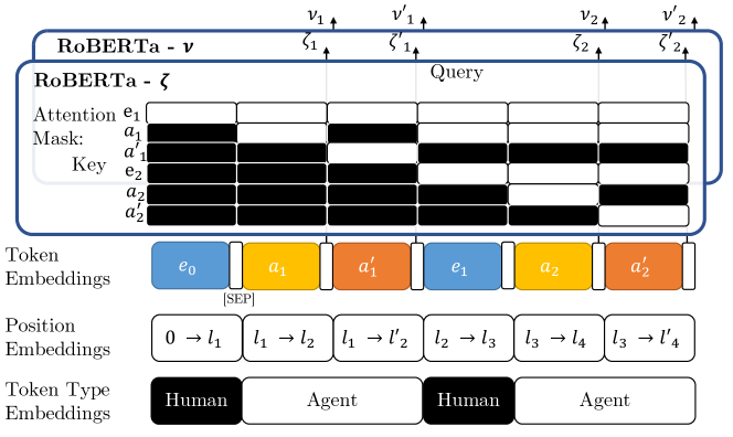
Figure 8: RoBERTa-$\zeta$ and RoBERTa-$\nu$

A.3 ENIGMA with regularized DICE

Algorithm 2 Dialog OPE using regularized DICE

1:Experience Dialog with rewards $\mathcal{D}=\{(h_{i}=\{e^{(i)}_{0},a^{(i)}_{1},e^{(i)}_{1},...,a^{(i)}_{T_{i}}\},r^{(i)})\}_{i=1}^{N}$, Target Policy $\pi$, Padding Length $T_{\rm max}$, Regularization function $f$, DICE hyper-parameters $\alpha_{\zeta}$, $\alpha_{R}$

2:Performance Estimation $\widehat{\rho}_{n}(\pi)$

3:$\zeta=\{$ RoBERTa-$\zeta,[\zeta_{{\rm pad},t}]_{1\leq t\leq T_{\rm max}}\}$,$\nu=\{$ RoBERTa-$\nu,[\nu_{{\rm pad},t}]_{1\leq t\leq T_{\rm max}}\}$, $\lambda$

4:

5:for  $({h}_{i},r^{(i)})$ in $\mathcal{D}$ do

6:     for $t$ in $1,\cdots,T_{i}$ do

7:         $\widetilde{a}_{t}^{(i)}\sim\pi(\{e^{(i)}_{0},a^{(i)}_{1},e^{(i)}_{1},...,e^{(i)}_{t-1}\})$ // Sample Action From Target Policy

8:     end for

9:end for

10:$\widetilde{\mathcal{D}}=\{(\widetilde{h}_{i}=e^{(i)}_{0},a^{(i)}_{1},e^{(i)}_{1},...,a^{(i)}_{T_{i}}\},r^{(i)})\}_{i=1}^{N}$

11:

12:while  Not Converged  do

13:     Sample Mini-Batch $\mathcal{B}\subset\widetilde{\mathcal{D}}$

14:     for  $(\widetilde{h}_{i},r^{(i)})$ in $\mathcal{B}$ do

15:         $\zeta^{(i)}_{0}=\zeta_{{\rm pad},T_{\rm max}}$,   $\nu^{(i)}_{0}=\nu^{\prime(i)}_{0}=\nu_{{\rm pad},T_{\rm max}}$ // infinite-horizon concatenation

16:         for $t$ in $1,\cdots,T_{i}$ do

17:              $\zeta_{t}^{(i)}=$ RoBERTa-$\zeta(e_{0}^{(i)},a_{1}^{(i)},...,a_{t-1}^{(i)},e_{t-1}^{(i)},a_{t}^{(i)})$

18:              $\nu_{t}^{(i)}=$ RoBERTa-$\nu(e_{0}^{(i)},a_{1}^{(i)},...,a_{t-1}^{(i)},e_{t-1}^{(i)},a_{t}^{(i)})$

19:              $\nu^{\prime(i)}_{t}=$ RoBERTa-$\nu(e_{0}^{(i)},a_{1}^{(i)},...,a_{t-1}^{(i)},e_{t-1}^{(i)},{\color[rgb]{1,0,0}\widetilde{a}_{t}^{(i)}})$

20:         end for

21:         for $t$ in $T_{i}+1,\cdots,T_{\rm max}$ do

22:              $\zeta_{t}^{(i)}=\zeta_{{\rm pad},t}$,   $\nu_{t}^{(i)}=\nu^{\prime(i)}_{t}=\nu_{{\rm pad},t}$ // add padding state

23:         end for

24:         $\ell_{i}=\frac{1}{T_{\rm max}}[\alpha_{R}\zeta^{(i)}_{T_{i}}r^{(i)}_{T_{i}}+\sum_{t=0}^{T_{\rm max}-1}[\zeta_{t}(\nu^{\prime(i)}_{t+1}-\nu^{(i)}_{t})+\lambda(\zeta^{(i)}_{t}-1)-\alpha_{\zeta}f(\zeta^{(i)}_{t})]]$

25:     end for

26:     $L_{D}(\zeta,\nu,\lambda)=\frac{1}{|\mathcal{B}|}\sum_{i\in\mathcal{B}}\ell_{i}$

27:     SGD update based on $\frac{\partial L_{D}}{\partial\nu}$,$\frac{\partial L_{D}}{\partial\lambda}$,$\frac{\partial-L_{D}}{\partial\zeta}$ (Gradient Reversal).

28:end while

29:

30:for  $({h}_{i},r^{(i)})$ in $\mathcal{D}$ do

31:     $\zeta_{i}=$ RoBERTa-$\zeta(e_{0}^{(i)},a_{1}^{(i)},...,a_{T_{i}-1}^{(i)},e_{T_{i}-1}^{(i)},a_{T_{i}}^{(i)})$

32:end for

33:Return $\widehat{\rho}_{n}(\pi)=\sum_{({h}_{i},r^{(i)})\in\mathcal{D}}\zeta_{i}r^{(i)}\big{/}\sum_{({h}_{i},r^{(i)})\in\mathcal{D}}\zeta_{i}$

Appendix B Experiment Set-Up

In the following experiments, we share the RoBERTa encoder for RoBERTa-$\zeta$ and RoBERTa-$\nu$. On the top of RoBERTa-$\zeta$ and RoBERTa-$\nu$, it is a two-layer fully connected neural network equipped with GeLU activation (Hendrycks and Gimpel, 2016) and the same hidden dimension as RoBERTa. The RoBERTa encoder is initialized from RoBERTa-base checkpoint (Liu et al., 2019). We simply use reverse gradients for the mini-max updates. We set learning rate as $2\times 10^{-4}$ and use inverse square root learning rate decay. We impose the gradient norm clipping with the maximum norm $\left\lVert\cdot\right\rVert_{2}\leq 10$. We use $100$ times larger learning rate for optimizing $\lambda$, $2$ times larger learning rate for RoBERTa-$\nu$. In (3.2), we set $\alpha_{\zeta}=1$, $f(x)=x^{2}$ as suggested in Yang et al. (2020). We maintain $\zeta\geq 0$ by adding a square activation at the end of RoBERTa-$\zeta$. The source code is built based on Transformers (Wolf et al., 2019), AirDialog (Wei et al., 2018), and ParlAI (Miller et al., 2017). All experiments are conducted on a machine with $8\times$ V100 GPUs on Google Cloud.

Appendix C Transformer-Based Agents for AirDialog

Seller Agent Transformer Architecture There are four components for the encoder: ticket encoder, reservation encoder, dialog encoder, and task-specific heads (intent classification head and name classification head). All tickets and reservation are converted to natural languages. Noticing that, we always append a pseudo ticket in the ticket database representing “no ticket found” situation. The architecture is illustrated in Figure 9.

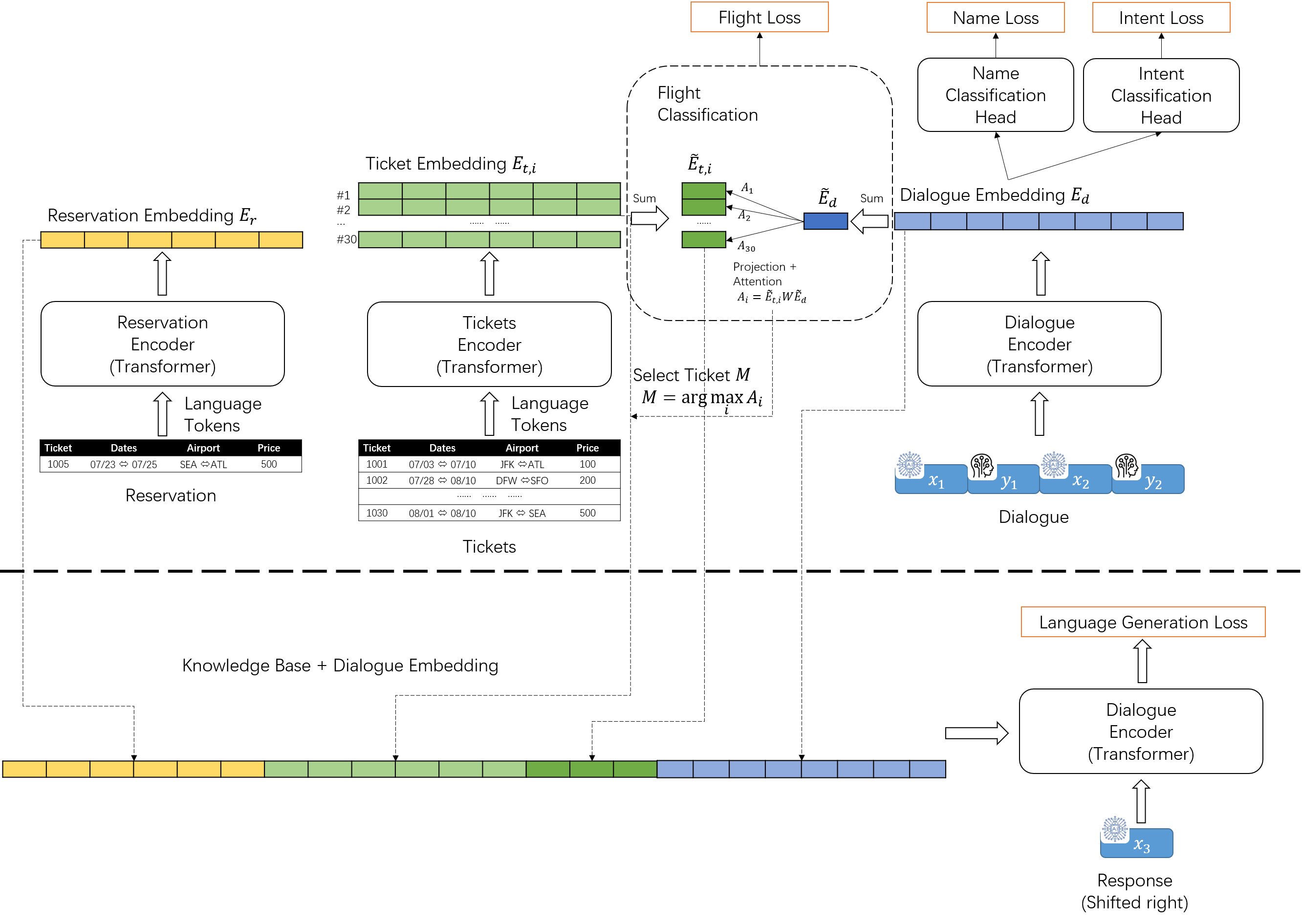
Figure 9: Transformer-based Seller Agent

Customer Agent Transformer Architecture There are two components for the encoder: intent encoder, reservation encoder. All intents are converted to natural languages. The architecture is illustrated in Figure 10.

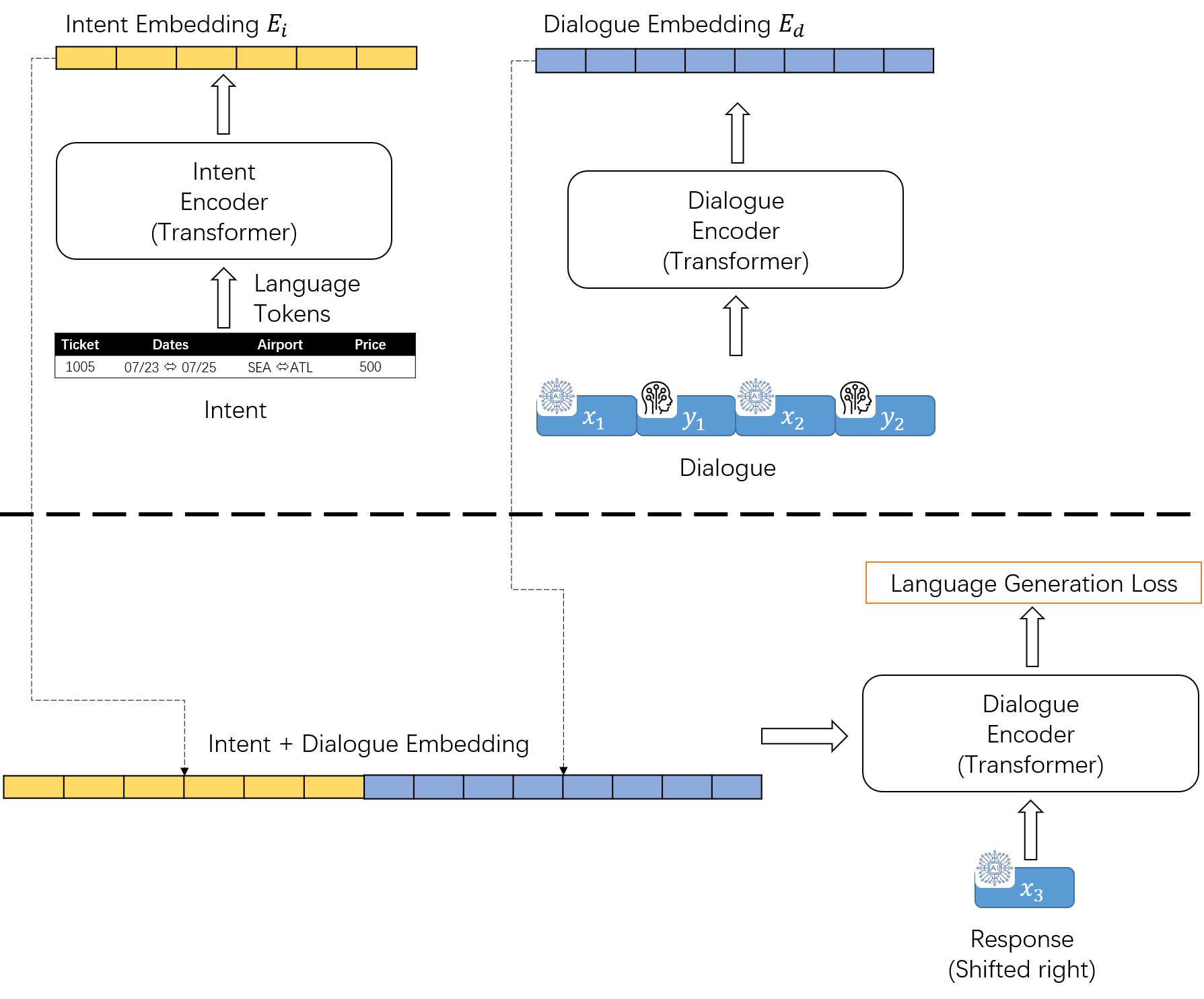
Figure 10: Transformer-based Customer Agent

Training Objective Besides the language generation loss $\mathcal{L}_{l}$, the training objective for seller consists of three parts: name loss, flight loss, intent loss:

$$\min_{\theta}\mathcal{L}_{s}(\theta)=\mathcal{L}_{l}(\theta)+\lambda_{n}\mathcal{L}_{\textrm{name}}(\theta)+\lambda_{f}\mathcal{L}_{\textrm{flight}}(\theta)+\lambda_{i}\mathcal{L}_{\textrm{intent}}(\theta)$$ (13)

The customer agent is trained with normal language generation loss.

Benchmark We compare the proposed model with the current AirDialog RNN baseline (Wei et al., 2018). As can be seen, the agent used in this paper are significantly stronger than the baseline agent used in Wei et al. (2018).

Table 5: Benchmark of the proposed transformer based agent. ‘C’ means customer, ‘S’ means seller. Reward, Name, Flight, status are the task-specific scores obtained from self-play evaluation.

Model	BLEU (C)	BLEU (S)	PPL (C)	PPL (S)	Reward	Name	Flight	Status
RNN	22.92	32.95	-	-	0.23	0.41	0.13	0.29
Ours	31.78	31.70	1.671	1.843	0.702	1.00	0.547	0.761

Hyper-Parameters For training 24 seller agents used in Section 4, we varies the size of training data (number of training dialogs) from $5K$ to the full size and varies $\lambda_{i}$ and $\lambda_{f}$ from $0.0001$ to $1$. For training the customer agent used in self-play evaluation, we use the full training data and tune the hyperparameters based on the BLEU score evaluated using the validation set.

Human Evaluation The human evaluation is collected from 20 different Ph.D. students majored in Math/Stats/CS/IEOR. We provide detailed guidelines to the human evaluator that they have to speak to the agents with similar tone. Figure 11 presents the screen shots of the human evaluation software.

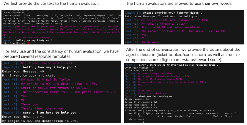
Figure 11: Screen Shots of Human Evaluation Software

Appendix D Additional Experiment

D.1 AirDialog

Regression Plot

We present the regression plot for the full setting in Figure 12 and for the selected agent in Figure 13.

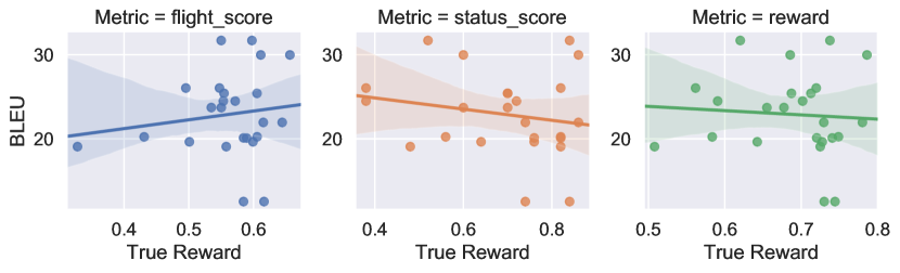
(a) BLEU vs. Human Evaluation

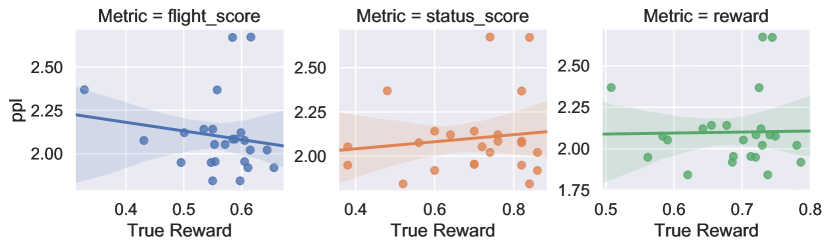
(b) PPL vs. Human Evaluation

(c) SPE vs. Human Evaluation

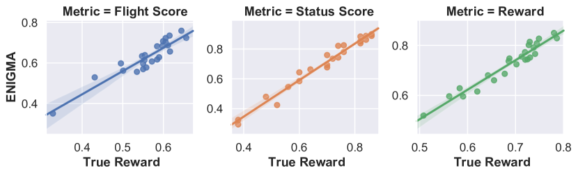
(d) ENIGMA vs. Human Evaluation

Figure 12: Regression Plot. The x-axis is the average reward obtained by chatting with human. The y-axis is BLEU/PPL/the reward estimated by ENIGMA. Different colors denotes different type of rewards (flight score, status score, and overall reward). The solid line is obtained by linear regression and the shaded region indicates $95\%$ confidence interval. (see more in seaborn packages).

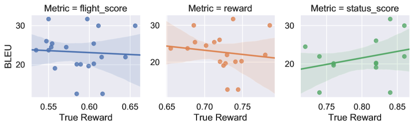
(a) BLEU vs. Human Evaluation

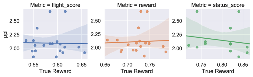
(b) PPL vs. Human Evaluation

(c) SPE vs. Human Evaluation

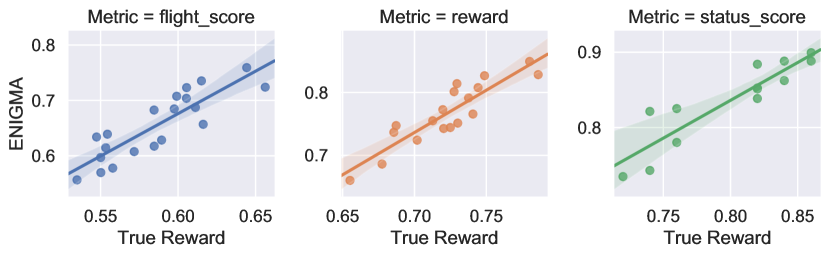
(d) ENIGMA vs. Human Evaluation

Figure 13: Regression Plot for “selected agent” Setting. The x-axis is the average reward obtained by chatting with human. The y-axis is BLEU/PPL/the reward estimated by ENIGMA/Self-Play Evaluation (SPE). Different colors denotes different type of rewards (flight score, status score, and overall reward). The solid line is obtained by linear regression and the shaded region indicates $95\%$ confidence interval. (see more in seaborn packages).

Training Curves

We show the training curves of the ENIGMA in Figure 14. Here four models are presented, the best model (ranked $100\%$), model ranked as $50\%$, model ranked as $25\%$ and the worst model (ranked $0\%$). As can been seen the estimated reward estimation converges steadily to it’s true values.

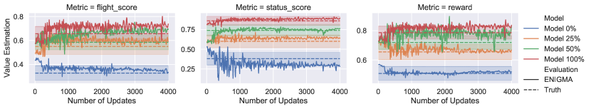
Figure 14: Learning curve for AirDialog. The x-axis is the number of mini-max updates, while y-axis is the estimated values. The straight line is the true reward, while the shaded region denotes the $90\%$ confidence interval. The true reward and the confidence interval is obtained via different evaluation chats between the agents and the environment (model/human). Different colors denotes different agents.

Ablation Study

Here we provide large figures (Figure 15 and Figure 16) for the ablation study mentioned in Section 4.

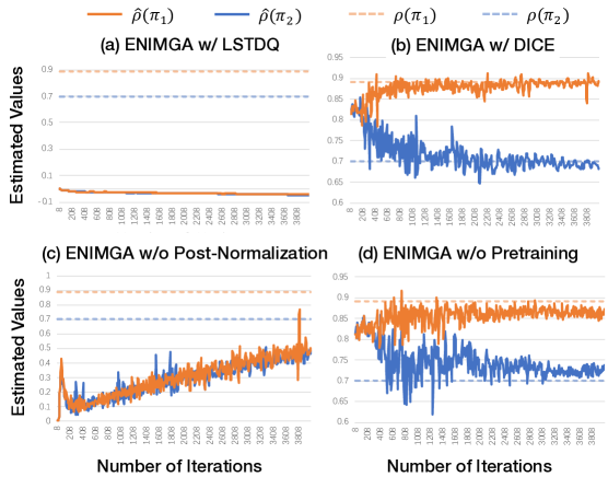
Figure 15: Reward estimation of two target agents ($\pi_{1}$ and $\pi_{2}$) vs. # of iterations. Dotted lines represents true rewards.

Figure 16: Loss value of two target agents during mini-max optimization.

D.2 Additional Results for Rule-Based Agents of AirDialog

$\bullet$ Rule-Rule (R-R): Both customer and seller agents are rule based. We fix the customer rule-based model and construct and evaluate 6 seller agents. The strongest agent can perfectly interpret the intent of rule-based customers. While the weaker agents interprets the intent with different levels of noise. The learning curve is presented in Figure 17.

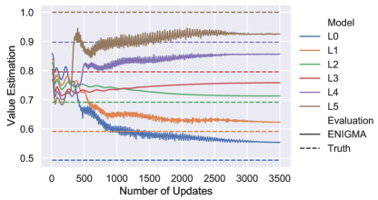
Figure 17: Learning Curve under Rule-Rule setting

Table 6: The correlation between two metrics. Each column is a task completion score obtained by interacting with the environments under R-R setting. Each row is an automatic metric.

Setting	Method	Pearson Correlation			Spearman’s Rank Correlation
		Flight Score	Status Score	Reward	Flight Score	Status Score	Reward
R-R	BLEU	0.1981	-0.0067	0.0980	0.1525	0.0009	0.0924
	ppl	-0.1584	-0.0610	-0.1209	-0.2475	-0.1060	-0.1178
	ENIGMA	0.9687	0.9947	0.9874	0.8800	0.9872	0.9574

D.3 ConvAI2

Training Curves.

Similar to the AirDialog dataset, we also show the training curves for the agents ranked at $100\%$, $50\%$, $25\%$, $0\%$ in Figure 18. ENIGMA also converges steadily to the true values within a resonable error.

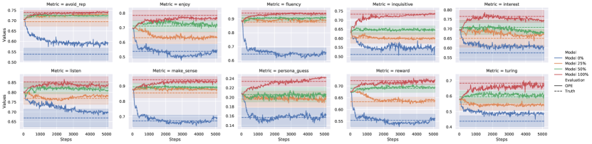
Figure 18: Learning curve for ConvAI2. The x-axis is the number of mini-max updates, while y-axis is estimated values. The straight line is the true reward, while the shaded area denotes the $95\%$ confidence interval. The true reward and the confidence interval is obtained via different evaluation chats between the agents and human. Different colors denotes different agents.

Regression Plot.

We present the regression plot for the all 10 metrics in setting in Figure 19. The corresponding corresponding correlation is presented in Table 7. For comparison, we present the regression plot for self-play evaluation in Figure 20.

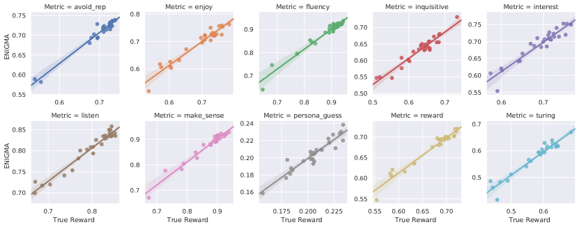
Figure 19: ENIGMA vs. Human Evaluation for ConvAI2. The x-axis is the average reward obtained by chatting with human. The y-axis it the reward estimated by ENIGMA. Different colors represent different language quality metrics. The solid line is obtained by simple linear regression.

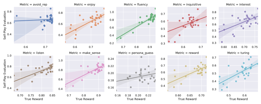
Figure 20: Self-Play Evaluation vs. Human Evaluation for ConvAI2. The x-axis is the average reward obtained by chatting with human. The y-axis it the reward estimated by self-play evaluation Different colors represent different language quality metrics. The solid line is obtained by simple linear regression.

Experience Data.

To analysis how many human-model evaluation dialogs are needed, we analysis ENIGMA error under different sizes of the experience data. For ConvAI2, we compare the error for using $100\%$ data, $50\%$ data and $10\%$ data. As shown in Table 7 and Figure 21, when we use half of the data, the error is similar to the one using full data. If we only use $10\%$ data, ENIGMA becomes very inaccurate. OPE under low resource setting remains very challenging.

In Figure 21, we study the estimation error under different sizes of the experience data. As can be seen, when using $50\%$ data, the reward value estimation is very similar to the one of using full data. When using only $10\%$ data, the error is larger and ENIGMA has lower correlation with the true reward.

Table 7: The correlation between different metrics and ENIGMA estimation. Each column is each average language quality score obtained by chatting with human. Different rows represent different experience data ENIGMA used.

Pearson Correlation
Setting	Avoid Rep.	Enjoy	Fluency	Inquisitive	Interest
Full Data	0.9792	0.9661	0.9767	0.9584	0.9488
$50\%$ Data	0.9573	0.9046	0.9550	0.9237	0.8644
$10\%$ Data	0.9266	0.6595	0.8910	0.8286	0.5052
Selected Data	0.6944	0.6759	0.7762	0.5605	0.5820
Setting	Listen	Make Sense	Persona	Reward	Turing
Full Data	0.9754	0.9788	0.9415	0.9773	0.9637
$50\%$ Data	0.8971	0.9585	0.8770	0.9374	0.8506
$10\%$ Data	0.7455	0.8100	0.4544	0.8240	0.6825
Selected Data	0.5520	0.7402	0.6879	0.6968	0.5394
Spearman’s rank correlation
Setting	Avoid Rep.	Enjoy	Fluency	Inquisitive	Interest
Full Data	0.8905	0.9070	0.9178	0.8717	0.9210
$50\%$ Data	0.7558	0.7980	0.6651	0.8482	0.7727
$10\%$ Data	0.4128	0.6147	0.6492	0.6335	0.4713
Selected Data	0.5138	0.5561	0.4522	0.3168	0.6027
Setting	Listen	Make Sense	Persona	Reward	Turing
Full Data	0.9240	0.9448	0.9205	0.9485	0.9213
$50\%$ Data	0.7784	0.8647	0.8293	0.7750	0.7026
$10\%$ Data	0.3914	0.5096	0.3651	0.5774	0.5893
Selected Data	0.4585	0.6126	0.5844	0.6672	0.4259

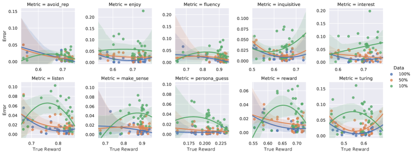
Figure 21: Error Analysis on Convai2 under different data size. The x-axis is the true average reward. The y-axis is the ENIGMA error. The solid line is the fitted quadratic function. Blue, orange, green colors represent $100\%$, $50\%$, $10\%$ datasets respectively.

A More Challenging Setting.

Considering that some target agents are similar to the behavior policies with only slight difference in the way of decoding, they might yield very the similar dialog when the human acts in the same way. Specifically, in the data collection process, the target model might yield the responses that are very similar to the ones of the behavior policy for all turns in the dialog: ${\rm EditDistance}(a_{t},a^{\prime}_{t})\leq 15~{}~{}\forall 0\leq t\leq T$. For a more realistic setting, we consider removing these highly overlapped dialogs after the data collection process. This setting is very challenging that the target policy behavior is less covered by the experience data and ENIGMA can only hopefully generalize via pre-trained RoBERTa. The results are shown in Figure 22 and Table 7. As can be seen, this setting remains challenging as the Pearson correlation is between $0.5$ and $0.8$. For comparison, we present the regression plot for self-play evaluation using this challenging subset of the experience data in Figure 23.

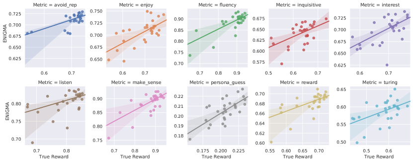
Figure 22: ENIGMA vs. Human Evaluation for ConvAI2 under the challenging setting. The x-axis is the average reward obtained by chatting with human. The y-axis it the reward estimated by ENIGMA. Different colors represent different language quality metrics. The solid line is obtained by simple linear regression.

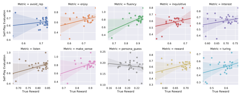
Figure 23: Self-Play Evaluation vs. Human Evaluation for ConvAI2 under the challenging setting. The x-axis is the average reward obtained by chatting with human. The y-axis it the reward estimated by self-play evaluation. Different colors represent different language quality metrics. The solid line is obtained by simple linear regression.

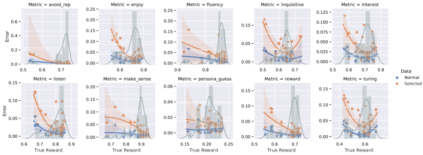
Figure 24: ENIGMA Error Comparison between using normal and selected challenging experience data on ConvAI2. The x-axis is the true average reward. The y-axis is the ENIGMA error. The solid line is the fitted quadratic function. The histogram is the empirical distribution of the rewards of all the experience data. Orange represents challenging dataset, and blue represents normal dataset.

We remark that such experiments can also be done for AirDialog. However, due to the limitation that most agents are just learning template responses due to the goal-oriented nature, removing overlapped dialogs results in an extremely incomplete experience dataset. For example, most “cancelation” dialogs will be removed since they are very simple and basically the same for different agents. As a result ENIGMA can not make a reasonable estimation due to the highly incomplete experience data.

Figure 24 compares the error of ENIGMA between using the normal experience data and the selected challenging one. As can be seen, the error using the selected data is larger particularly for the agents with exceptionally low/high true reward. That indicates the problem of the lack of dialog coverage is exaggerated under the challenging setting, while the ENIGMA estimation remains accurate when there is sufficient dialog coverage.

Comparison to Automatic Hand-crafted Metrics.

We compare ENIGMA with other automatic hand-crafted metrics proposed in See et al. (2019). For a more intuitive comparison, we use heat map and box plot to visualize the correlations between different automatic evaluation metrics and different human evaluation metrics. As can be seen in Figure 25 and Figure 26, most hand-crafted metrics have relatively low correlation to human evaluation metrics. The only exception is the “question marks” automatic metrics for inquisitive human evaluation metric. Some hand-crafted metrics have high Pearson correlation to some human evaluation metrics, while the corresponding Spearman’s rank correlation is low. The reason is that they can easily identify some extremely good/bad agents while they are less effective for identifying agents with similar performance.

Comparison to BLEU, BLEURT, and BERTscore. We compare ENIGMA with other automatic single-turn language quality metrics in Figure 25: BLEU, BLEURT (Sellam et al., 2020), and BERTscore (Zhang et al., 2019). As can be seen, these metrics only have high correlation to certain human evaluation metrics and low correlation to other metrics. Note that, we do not compare the perplexity as the agents rely on complicated decoding methods (See et al., 2019) and perplexity does not take decoding into consideration.

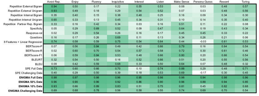
(a) Pearson Correlation

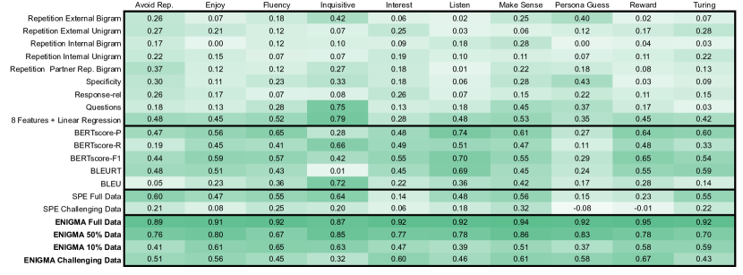
(b) Spearman’s Rank Correlation

Figure 25: Heat map for correlation between different automatic evaluation metrics and different human evaluation metrics. Different rows represent different automatic metrics. Different column represent different human evaluation metrics.

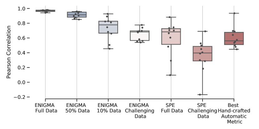
(a) Pearson Correlation

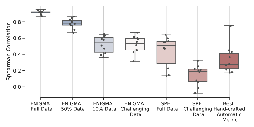
(b) Spearman’s Rank Correlation

Figure 26: Box plot of performance. Each box corresponds to each method. There are 10 points for each box representing correlations to 10 different human evaluation metrics.

D.4 Error Analysis

We analyze the detailed errors to identify the error pattern for better understand the limit of ENIGMA. We calculate the absolute difference between the estimation and the true average reward. The results are summarized in Figure 27. A common pattern we see in ConvAI2 is that, when the true average reward is too high or too low, the ENIGMA becomes less accurate. One possible reason for that is the lack of samples of dialogs with the extreme rewards in the experience data. We empirically verify this conjecture by comparing the the error with the reward distribution in the experience data in Figure 27. For AirDialog, such pattern is not obvious. That is because the quality of the decision module is more important to the agent performance for this task completion scores. As a result, even performance of the target agent is much higher/lower than the experience data, as long as they share similar languages, ENIGMA can estimate the performance accurately.

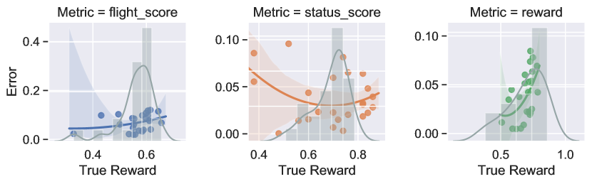
(a) AirDialog

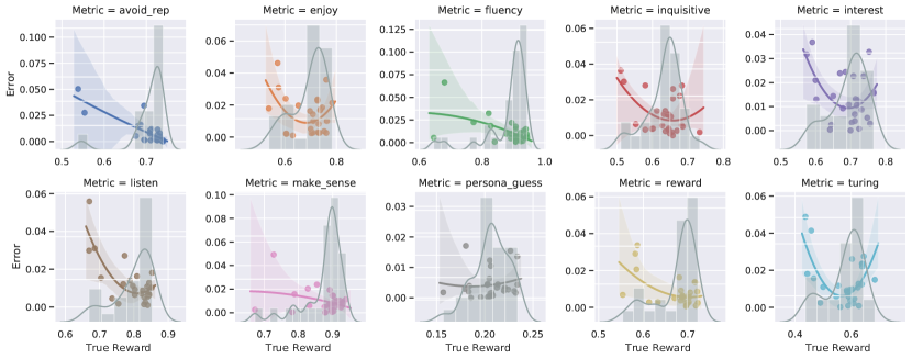
(b) ConvAI2

Figure 27: Error Analysis on AirDialog and ConvAI2. The x-axis is the true reward. The y-axis is the Estimation error. The solid line is the fitted quadratic function. The histogram is the empirical distribution of the true rewards of all the experience data.

D.5 Embedding Visualization

In Figure 28, we present the t-SNE plots for the embedding of the state-action pairs from the behavior experience data and the target policy. The two sets of embeddings provided by the pre-trained language models are largely overlapped with rich semantic information. On the other hand, the embeddings provided by a randomly initialized model spread over the entire high-dimensional space.

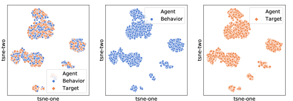
(a) Initialized from RoBERTa-base.

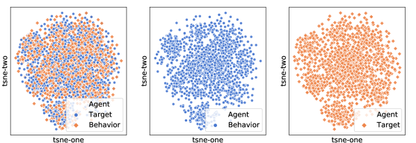
(b) Random initialization.

Figure 28: t-SNE Plots for contextual embedding extracted from RoBERTa-$\zeta$ and RoBERTa-$\nu$ on AirDialog.

Appendix E Automatic Dialog Evaluation Comparison

Table 8: Comparison between current automatic evaluation approaches. Part of the table is collected from two comprehensive surveys Finch and Choi (2020); Deriu et al. (2020). Red: Drawback; Green: Advantage.

Method	Criterion	Dynamic (RL)	Model Free	Experience Data	Behavior Policy Similar to Target Policy	Behavior Agnostic	Description / Examples
BLEU, Perplexity,METEOR,ROUGE
Papineni et al. (2002); Brown et al. (1992); Banerjee and Lavie (2005); Lin (2004); Galley et al. (2015)	Language Quality Score	No	N/A	Human-Human	Yes	N/A	The most widely use metrics: Given a fixed dialog history, they compute heuristic scores / statistics based on comparing single turn response given by the model and reference human responses. E.g., BLEU, perplexity
Mitchell and Lapata (2008); Rus and Lintean (2012); Forgues et al. (2014); Higashinaka et al. (2014); Xiang et al. (2014); Wieting et al. (2015); Gandhe and Traum (2016); Tao et al. (2017); Shimanaka et al. (2019); Zhang et al. (2019); Ghazarian et al. (2019); Li et al. (2020); Mehri and Eskenazi (2020); Gao et al. (2020); Lan et al. (2020); Pang et al. (2020); Zhang et al. (2020a); Yuma et al. (2020); Zhao et al. (2020); Sai et al. (2020)	Language Quality Score	No	N/A	Human-human experience data or specially designed data.	Yes (Implicitly)      Although they do not explicitly require such similarity, the single-turn responses of models trained from the same data are usually similar to human responses.	N/A	Given a fixed dialog history, they compute some scores for single-turn response given by the model using an evaluator, e.g., pretrained word embeddings and pretrained language models. These method are the so-called “embedding-based metrics”. The evaluator usually require training on a large-scale text dataset. They may or may not depends on reference human responses. E.g. RUBER (Tao et al., 2017).
Lowe et al. (2017); Huang et al. (2020); Sellam et al. (2020)	Language Quality Score	No	N/A	Human-Human and Human-Model	Yes	N/A	Mostly the same as above. In addition, the data for training the evaluator includes human-model experience data to improve performance. E.g., ADEM Lowe et al. (2017).
Hemphill et al. (1990); Williams et al. (2013)	Task Completion Score	No	N/A	Human-Human	No	N/A	They compute task related score of task-specific actions (e.g., intent detection) given by the model for a fixed complete dialog. These can only be used to test classification / information retrieval module. E.g., Intent Detection Accuracy.
Wei et al. (2018)	Task Completion Score	Yes	No	Human-Human and/or Human-Model	Yes (Implicitly)	N/A	They compute task related score of task-specific actions (e.g., intent detection) given by the model for a dialog that is obtained by interaction with a user simulator. E.g., Self-Play Evaluation Wei et al. (2018).
Ghandeharioun et al. (2019)	Language Quality Score	Yes	No	Human-Model	Yes	N/A	Basically the same as above. In addition to modeling human responses, they usually require modeling human reward function. E.g., Self-Play Evaluation Ghandeharioun et al. (2019).
Inverse Proportional Score E.g., Horvitz and Thompson (1952); Wang et al. (2020a); Precup (2000) (not practical for dialog )	Both	Yes	Yes	Human-Model	Yes	No (not practical for dialog)	Directly model the performance under the interaction environment using experience collected from known probabilistic models. E.g., Inverse Proportional Score.
ENIGMA	Both	Yes	Yes	Human-Model	Yes	Yes	Directly model the performance under interaction environment using experience collected from unknown distribution. E.g., Q-Learning, ENIGMA.

E.1 Static Methods

As can be seen, most previous methods only focus on evaluating language quality for single-turn response of a fixed context. These methods can not evaluate agents under interactive context. As a result, they can not be extended to goal-oriented dialogs.

For goal-oriented dialogs, the static evaluation methods are very limited. The static methods can only evaluate the model actions to a fixed complete dialog, e.g., intent detection.

Comparison to Meena Paper (Adiwardana et al., 2020): 1. They only show that PPL correlates with one specific metric: Sensibleness and Specificity Average. We consider a wide range of metrics for both task-completion scores and dialog quality scores (listed in Table 7). No evidence shows PPL correlates well with most metrics. 2. They draw the conclusion using only 7 chatbots. This conclusion is not statistically reliable, i.e. for $R^{2}=0.93$ with 7 data points, the $95\%$ confident interval is $0.64\leq R^{2}\leq 0.99$. On the other hand, we use 24/29 agents. With 24 data points, the $95\%$ CI is $0.87\leq R^{2}\leq 0.96$, which is much more reliable.

E.2 Dynamic Methods

Previous dynamic methods under RL framework are based on self-play evluation, which requires learning the environment, i.e, human. As discussed in the main paper, learning a human model is significantly beyond the current technical limit.

ENIGMA overcome learning the environment by directly modeling the performance of agents.

E.3 Information Theoretic Limit

The common limitation of all existing methods is that they require similarity between the target policy and behavioral policies, so that the experience data can cover sufficient interaction patterns between the target policy and human.

For example, BLEU score requires the agent response being similar to the reference response. Another example is ADEM (Lowe et al., 2017), they include the target policy into the experience data collection to achieve decent performance ($0.37$ Pearson correlation to human ratings). If the target policy is excluded from the behavior policies, ADEM only achieves $0.13$ Pearson correlation, which is even lower than the one between dialog length and human ratings $0.27$.

For static single-turn evaluation for language quality, one might satisfy the requirement by just using human as the behavior policy and large-scale diverse experience data. That is because the single-turn responses of the target model have a very similar pattern to the human responses, as they are usually trained to mimic one-turn human response. However, high similarity of responses between the target model and human requires a very strong target model trained with large-scale data, which is not practical in most settings. Some existing work try to alleviate such requirement and increase the coverage of experience data by external knowledge graph (Huang et al., 2020) and synthetic samples (Sellam et al., 2020). We remark that although the static methods only require single-turn similarity between behavior and target policies, their empirical performance is unsatisfactory comparing with multi-turn interactive human evaluation (Ghandeharioun et al., 2019).

In multi-turn interactive evaluation, we can not just use human as the behavior policy especially for goal-oriented dialogs. That is because the multi-turn behavior of the target model is very different from the human behavior. Take Airdialog as an example, human agents can always book the correct tickets while the target model may fail for many times.

Such a limitation is the theoretical requirement of bounded state-action density ratio between target and behavior policies, which has been discussed in many off-policy evaluation literature Wang et al. (2020b); Xie et al. (2019).

Due to such theoretical limitation, a large amount of human-model interactive evaluation data is needed to study automatic interactive evaluation. However, most evaluation logs are not publicly available, and research in this direction has largely lagged behind. To the best of our knowledge, ConvAI2 (See et al., 2019) is the only public comprehensive human-model interactive evaluation data. Therefore, we recommend that the research community release human-model interaction evaluation data to promote dialog evaluation/learning research and benefit the entire community.

References

- Adiwardana et al. (2020) Adiwardana, D., Luong, M.-T., So, D. R., Hall, J., Fiedel, N., Thoppilan, R., Yang, Z., Kulshreshtha, A., Nemade, G., Lu, Y. et al. (2020). Towards a human-like open-domain chatbot. arXiv preprint arXiv:2001.09977.
- Banerjee and Lavie (2005) Banerjee, S. and Lavie, A. (2005). Meteor: An automatic metric for mt evaluation with improved correlation with human judgments. In Proceedings of the acl workshop on intrinsic and extrinsic evaluation measures for machine translation and/or summarization.
- Brown et al. (1992) Brown, P. F., Della Pietra, S. A., Della Pietra, V. J., Lai, J. C. and Mercer, R. L. (1992). An estimate of an upper bound for the entropy of english. Computational Linguistics, 18 31–40.
- Chen et al. (2018) Chen, Z., Li, X., Yang, L. F., Haupt, J. and Zhao, T. (2018). On landscape of lagrangian functions and stochastic search for constrained nonconvex optimization. arXiv preprint arXiv:1806.05151.
- Dai et al. (2017) Dai, B., Shaw, A., He, N., Li, L. and Song, L. (2017). Boosting the actor with dual critic. arXiv preprint arXiv:1712.10282.
- Deriu et al. (2020) Deriu, J., Rodrigo, A., Otegi, A., Echegoyen, G., Rosset, S., Agirre, E. and Cieliebak, M. (2020). Survey on evaluation methods for dialogue systems. Artificial Intelligence Review 1–56.
- DeVault et al. (2011) DeVault, D., Leuski, A. and Sagae, K. (2011). Toward learning and evaluation of dialogue policies with text examples. In Proceedings of the SIGDIAL 2011 Conference.
- Devlin et al. (2018) Devlin, J., Chang, M.-W., Lee, K. and Toutanova, K. (2018). Bert: Pre-training of deep bidirectional transformers for language understanding. arXiv preprint arXiv:1810.04805.
- Dinan et al. (2020) Dinan, E., Logacheva, V., Malykh, V., Miller, A., Shuster, K., Urbanek, J., Kiela, D., Szlam, A., Serban, I., Lowe, R. et al. (2020). The second conversational intelligence challenge (convai2). In The NeurIPS’18 Competition. Springer, 187–208.
- Duan and Wang (2020) Duan, Y. and Wang, M. (2020). Minimax-optimal off-policy evaluation with linear function approximation. arXiv preprint arXiv:2002.09516.
- Dziri et al. (2019) Dziri, N., Kamalloo, E., Mathewson, K. W. and Zaiane, O. (2019). Evaluating coherence in dialogue systems using entailment. arXiv preprint arXiv:1904.03371.
- Finch and Choi (2020) Finch, S. E. and Choi, J. D. (2020). Towards unified dialogue system evaluation: A comprehensive analysis of current evaluation protocols. arXiv preprint arXiv:2006.06110.
- Forgues et al. (2014) Forgues, G., Pineau, J., Larchevêque, J.-M. and Tremblay, R. (2014). Bootstrapping dialog systems with word embeddings. In Nips, modern machine learning and natural language processing workshop, vol. 2.
- Galley et al. (2015) Galley, M., Brockett, C., Sordoni, A., Ji, Y., Auli, M., Quirk, C., Mitchell, M., Gao, J. and Dolan, B. (2015). deltableu: A discriminative metric for generation tasks with intrinsically diverse targets. arXiv preprint arXiv:1506.06863.
- Gandhe and Traum (2016) Gandhe, S. and Traum, D. (2016). A semi-automated evaluation metric for dialogue model coherence. In Situated Dialog in Speech-Based Human-Computer Interaction. Springer, 217–225.
- Gao et al. (2020) Gao, X., Zhang, Y., Galley, M., Brockett, C. and Dolan, B. (2020). Dialogue response ranking training with large-scale human feedback data. arXiv preprint arXiv:2009.06978.