Sparse Array Transceiver Design for Enhanced Adaptive Beamforming in MIMO Radar

Abstract

Sparse array design aided by emerging fast sensor switching technologies can lower the overall system overhead by reducing the number of expensive transceiver chains. In this paper, we examine the active sparse array design enabling the maximum signal to interference plus noise ratio (MaxSINR) beamforming at the MIMO radar receiver. The proposed approach entails an entwined design, i.e., jointly selecting the optimum transmit and receive sensor locations for accomplishing MaxSINR receive beamforming. Specifically, we consider a co-located multiple-input multiple-output (MIMO) radar platform with orthogonal transmitted waveforms, and examine antenna selections at the transmit and receive arrays. The optimum active sparse array transceiver design problem is formulated as successive convex approximation (SCA) alongside the two-dimensional group sparsity promoting regularization. Several examples are provided to demonstrate the effectiveness of the proposed approach in utilizing the given transmit/receive array aperture and degrees of freedom for achieving MaxSINR beamforming.

I Introduction

Non-uniform sparse arrays have emerged as an effective technology which can be deployed in various active and passive sensing modalities, such as acoustics and radio frequency (RF) applications, including GPS[1]. Fundamentally, sparse array design seeks optimum system performance, under both noise and interference, while being cognizant of the limitations on cost and aperture. Within the RF beamforming paradigm, maximizing the signal to interference plus noise ratio (SINR) amounts to concurrently optimizing the array configuration and beamforming weights. Equivalently, the problem can be cast as continuously selecting the best antenna locations to deliver MaxSINR under time-varying environment. In lieu of constantly moving antennas to new positions, a more practical and feasible approach is to have a uniform full array and then switch among antennas with a fixed number of front-end chains, yielding the MaxSINR sparse beamformer for a given environment.

The above environment-dependent approach differs from the environment-independent sparse array design that seeks to increasing the spatial autocorrelation lags and maximizing the contiguous portion of the coarray aperture for a limited number of sensors. The main task, therein, is to enable DOA estimation involving more sources than the physical sensors [2, 3, 4, 5, 6]. For beamforming applications, the environment-independent design criteria typically strives to achieve desirable beampattern characteristics such as broad main lobe and minimum sidelobe levels and frequency invariant beampattern for wideband design [7, 8, 9, 10, 11, 12].

Environment-dependent sparse receive beamformer striving to achieve MaxSINR can potentially provide sparse configurations that improve target detection and estimation accuracy [13, 14, 15, 16, 17, 18, 19, 20, 21]. In this paper, we consider MaxSINR receive beamformer design for MIMO radar operation. The beamformer design, in this case, jointly selects the optimum transmit and receive sensor locations for implementing an efficient receive beamformer. We assume that transmit sensors emit orthogonal waveforms. The MIMO radar implementing sensor-based orthogonal transmit waveforms does not benefit from coherent transmit processing gain achieved when using directional beamforming. In this context, the proposed approach is fundamentally different from the parallel sparse array MIMO beamforming designs, which primarily rely on optimizing the transmit sensor locations and the corresponding correlation matrix of the transmit waveform sequence [22, 23, 24, 25, 26]. The proposed approaches, therein, maximize the transmitted signal power towards the perspective target locations while minimizing the cross-correlation of the target returns to achieve efficient receive beamforming characteristics. Moreover, existing design schemes essentially pursue an uncoupled transmit/receive design which is in contrast to the proposed approach that incorporates sparse receiver design in conjunction with transmit array optimization.

The proposed transceiver beamforming design problem, in essence, translates to configuring the transmit/receive array with the corresponding optimum receiver beamforming weights. To this end, we pursue a data dependent approach that jointly optimizes the beamforming sensor positions and weights. The optimization only requires the knowledge of the perspective desired source locations and does not assume any knowledge of the interfering sources. We optimally select $M_{t}$ from $M$ transmitters and $N_{r}$ from $N$ receivers. Such selection is a binary optimization problem, and is NP-hard. In order to avoid extensive computations associated with enumeration of all possible array configurations, we apply convex relaxation. The design problem is posed as SCA with two-dimensional reweighted mixed $l_{1,2}$-norm penalization to jointly invoke sparsity in the transmit and receive dimensions.

The rest of the paper is organized as follows: In the next section, we state the problem formulation for the MIMO beamformer design in the case of a pre-specified array configuration. Section III elaborates on the sparse array design by semidefinite relaxation to jointly find the optimum sparse transmit/receive array geometry. In the subsequent section, simulations are presented to demonstrate the offerings of the proposed sparse array transmit design. The paper ends with concluding remarks.

II Problem Formulation

We consider a MIMO radar with $M$ transmitters and $N$ receivers illuminating the scene through omni-directional beampattern. This is typically achieved through emissions of orthogonal waveforms across the transmit array. Specifically, we pursue a co-located MIMO arrangement with the transmit and receive arrays in close vicinity. As such, a far-field source is presented by equal angles of departure and arrival. Consider $K$ target sources arriving from $\{\theta_{s,k}\}$. The received baseband data $\mathbf{x}(n)\in\mathbb{C}^{MN\times 1}$ after matched filtering at the $N$ element uniformly spaced receiver array at time instant $n$ is given by,

$$\mathbf{x}(n)=\sum_{k=1}^{K}s_{k}(n)\mathbf{b}(\theta_{s,k})+\sum_{l=1}^{L_{c}}c_{l}(n)\mathbf{b}(\theta_{j,l})+\sum_{q=1}^{Q}\mathbf{i}_{q}(n)+\mathbf{v}(n),$$ (1)

where, $s_{k}(n)\in\mathbb{C}$ is the $k$th reflected target signal. The extended steering vector $\mathbf{b}(\theta)$ of the virtual array is $\mathbf{b}(\theta)=\mathbf{a}_{t}(\theta)\otimes\mathbf{a}_{r}(\theta)$. In the case of uniform transmit and receive linear arrays with a respective inter-element spacing of $d_{t}$ and $d_{r}$, the transmit and receive steering vectors are given by,

$$\mathbf{a}_{t}(\theta)={}[1\,\,\,e^{j2\pi(d_{t}/\lambda)cos\theta}{}\\ \,.\,.\,.\,\,\,\,\,\,\,e^{j2\pi(M-1)(d_{t}/\lambda)cos\theta}]^{T},$$ (2)

and

$$\mathbf{a}_{r}(\theta)={}[1\,\,\,e^{j2\pi(d_{r}/\lambda)cos\theta}{}\\ \,.\,.\,.\,\,\,\,\,\,\,e^{j2\pi(N-1)(d_{r}/\lambda)cos\theta}]^{T}.$$ (3)

The variance of additive Gaussian noise $\mathbf{v}(n)\in\mathbb{C}^{MN\times 1}$ is $\sigma_{v}^{2}$ at the receiver output. There are $L_{c}$ interferences $c_{l}(n)$ mimicking target reflected signal and $Q$ narrowband interferences $\mathbf{i}_{q}(n)$ $\in\mathbb{C}^{MN\times 1}$. The latter is defined as the Kronecker product of the receiver steering vector $\mathbf{a}_{r}(\theta_{i,q})$ and the matched filtering output of the interference $\mathbf{j}_{q}(n)$ such that $\mathbf{i}_{q}(n)=\mathbf{j}_{q}(n)\otimes\mathbf{a}_{r}(\theta_{i,q})$. The received data vector $\mathbf{x}(n)$ is then linearly combined to maximize the output SINR. The output signal $y(n)$ of the optimum beamformer for MaxSINR is given by [27],

$$y(n)=\mathbf{w}^{H}\mathbf{x}(n)$$ (4)

where $\mathbf{w}$ is the beamformer weight at the receiver. The optimal solution $\mathbf{w}_{o}$ can be obtained by solving the optimization problem that seeks to minimize the interference power at the receiver output while preserving the desired signal. The constraint minimization problem can be cast as,

$$\underset{\mathbf{w}\in\mathbb{C}^{MN}}{\text{minimize}} \quad\mathbf{w}^{H}\mathbf{R_{x}}\mathbf{w},$$ (5)

s.t. $$\quad\mathbf{w}^{H}\mathbf{R}_{s}\mathbf{w}=1,$$

where the source correlation matrix is $\mathbf{R}_{s}$ $=$ $\sum_{k=1}^{K}\sigma_{s,k}^{2}$ $\mathbf{b}(\theta_{s,k})\mathbf{b}^{H}(\theta_{s,k})$, with $\sigma^{2}_{s,k}=E\{s_{k}(n)s_{k}^{H}(n)\}$ denoting the average received power from the $k$th target return. The data correlation matrix, $\mathbf{R}_{\mathbf{x}}\approx(1/T)\mathbf{x}(n)\mathbf{x}(n)^{H}$, is directly estimated from the $T$ received data snapshots. The solution to the optimum weights in (5) is given by $\mathbf{w}_{o}=\mathscr{P}\{\mathbf{R}_{\mathbf{x}}^{-1}\mathbf{R}_{s}\}$, with the operator $\mathscr{P}\{.\}$ representing the principal eigenvector of the input matrix. This optimum solution yields the MaxSINR, SINR_o, given by [27],

$$\text{SINR}_{o}=\Lambda_{max}\{\mathbf{R}^{-1}_{n}\mathbf{R}_{s}\},$$ (6)

which is the MaxSINR is the maximum eigenvalue ($\Lambda_{max}$) of the product of the two matrices, the inverse of interference plus noise correlation matrix and the desired source correlation matrix. It is clear that the resulting solution holds irrespective of the array configuration, whether the array is uniform or sparse. For the latter, the performance of MaxSINR beamformer is intrinsically tied to the array configuration. The sparse optimization of the above formulation is explained in the next section.

III Sparse array design

The separate sensor selection problem for a joint transmit and receive design is a combinatorial optimization problem and can’t be solved in polynomial time. We formulate the sparse array design problem by exploiting the structure of the received signal model and solve it by applying sequential convex approximation. To exploit the sparse structure of the joint transmit and receive sensor selection, we introduce a two dimensional $l_{1,2}$-mixed norm regularization to recover group sparse solutions. One dimension pertains to the transmitter sparsity, whereas the other sparsity pattern is associated with the receiver side. Moreover, this two-dimensional sparsity pattern is entwined and coupled, meaning that when one transmitter is discarded, all $N$ receiving data pertaining to this transmitter is zero. Similarly, the receiver is discarded only when its received data corresponding to all the $M$ transmitters is zero. The structure of the optimal sparse beamforming weight vector is elucidated in (7), where $\checkmark$ denotes a sensor location activated, or selected, and $\times$ denotes a sensor not activated.

$$\overbrace{\underbrace{\left(\begin{array}[]{@{}rrrr@{}}\checkmark\\ \times\\ \times\\ \checkmark\\ \vdots\\ \times\end{array}\right)}_{\text{(Tx 1 active)}}}^{\mathbf{w}(1,N)}\quad\overbrace{\underbrace{\left(\begin{array}[]{@{}rrrr@{}}\checkmark\\ \times\\ \times\\ \checkmark\\ \vdots\\ \times\end{array}\right)}_{(\text{Tx 2 active)}}}^{\mathbf{w}(N+1,2N)}\quad\overbrace{\underbrace{\left(\begin{array}[]{@{}rrrr@{}}\times\\ \times\\ \times\\ \times\\ \vdots\\ \times\end{array}\right)}_{(\text{Tx 3 inactive)}}}^{\mathbf{w}(2N+1,3N)}\quad\ldots\overbrace{\underbrace{\left(\begin{array}[]{@{}rrrr@{}}\checkmark\\ \times\\ \times\\ \checkmark\\ \vdots\\ \times\end{array}\right)}_{(\text{Tx $M$ active)}}}^{\mathbf{w}(N(M-1)+1,MN)}$$ (31)

In (7), each column vector denotes the receive beamformer weights for a fixed transmit location. It is noted that the optimal sparse beamformer, corresponding to the active transmit and receive locations, follows a group sparse structure along the transmit and receive dimensions (the consecutive $N$ sensors are discarded vertically or the consecutive $M$ sensors are discarded horizontally. It is evident that the missing transmit sensor at position $3$, for example, translates to the sparsity along all the corresponding $N$ entries of $\mathbf{w}$ ($N$ consecutive $\times$ vertically in (7)). Similarly, the group sparsity is also invoked across the received signals corresponding to all transmitters ($M$ consecutive $\times$ horizontally in (7)).

III-A Group Sparse solutions through SCA

The problem in (5) can equivalently be rewritten by swapping the objective and constraint functions as follows,

$$\underset{\mathbf{w\in\mathbb{C}}^{MN}}{\text{maximize}} \quad\mathbf{w}^{H}\bar{\mathbf{R}}_{s}\mathbf{w}$$ (32)

s.t. $$\quad\mathbf{w}^{H}\mathbf{R_{x}}\mathbf{w}\leq 1$$

where $\bar{\mathbf{R}}_{s}=-\mathbf{R}_{s}$. The sparse MIMO configuration of uniformly spaced receivers and transmitters with a respective inter-element spacing of $d_{r}$ and $d_{t}=Nd_{r}$ is employed for data collection. The covariance matrix $\mathbf{R_{x}}$ of the full receive virtual array can be then obtained by the matrix completion method proposed in [17].

The beamforming weight vectors are generally complex valued, whereas the quadratic functions are real. This observation allows expressing the problem with only real variables which is typically accomplished by replacing the correlation matrix $\bar{\mathbf{R}}_{s}$ by $\tilde{\mathbf{R}}_{s}$ and concatenating the beamforming weight vector accordingly [28],

$$\tilde{\mathbf{R}}_{s}=\begin{bmatrix}\text{real}(\bar{\mathbf{R}}_{s})&-\text{imag}(\bar{\mathbf{R}}_{s})\\ \text{imag}(\bar{\mathbf{R}}_{s})&\text{real}(\bar{\mathbf{R}}_{s})\\ \end{bmatrix},\tilde{\mathbf{w}}=\begin{bmatrix}\text{real}({\mathbf{w}})\\ \text{imag}({\mathbf{w}})\\ \end{bmatrix}$$ (33)

Similarly, the received data correlation matrix $\mathbf{R_{x}}$ is replaced by $\mathbf{\tilde{R}_{x}}$. The problem in (32) then becomes,

$$\underset{\mathbf{\tilde{w}\in\mathbb{R}}^{2MN}}{\text{minimize}} \quad\mathbf{\tilde{w}}^{{}^{\prime}}\tilde{\mathbf{R}}_{s}\mathbf{\tilde{w}},$$ (34)

s.t. $$\quad\mathbf{\tilde{w}}^{{}^{\prime}}\mathbf{\tilde{R}_{x}}\mathbf{\tilde{w}}\leq 1,$$

where ^′ denotes transpose operation. After expressing the constraint in terms of real variables, we convexify the objective function by utilizing the first order approximation iteratively,

$$\underset{\mathbf{\tilde{w}\in\mathbb{R}}^{2MN}}{\text{minimize}} \quad\mathbf{m}^{(k)}{{}^{\prime}}\mathbf{\tilde{w}}+b^{(k)},$$ (35)

s.t. $$\quad\mathbf{\tilde{w}}^{{}^{\prime}}\mathbf{\tilde{R}_{x}}\mathbf{\tilde{w}}\leq 1,$$

where, $\mathbf{m}^{(k)}$ and ${b^{(k)}}$, updated at the $k+1$ iteration, are given by $\mathbf{m}^{(k+1)}=2\tilde{\mathbf{R}}_{s}\mathbf{\tilde{w}}^{(k)},b^{(k+1)}=-\mathbf{\tilde{w}}^{(k)}{{}^{\prime}}\tilde{\mathbf{R}}_{s}\mathbf{\tilde{w}}^{(k)}$, respectively. Finally, to invoke sparsity in the beamforming weight vector, the re-weighted mixed $l_{1,2}$ norm is adopted primarily for promoting group sparsity,

$$\underset{\mathbf{\tilde{w}},\mathbf{c},\mathbf{r}}{\text{minimize}}\quad \quad\mathbf{m^{(k)}{{}^{\prime}}}\mathbf{\tilde{w}}+b^{(k)}+\alpha(\mathbf{p}^{{}^{\prime}}\mathbf{c})+\beta(\mathbf{q}^{{}^{\prime}}\mathbf{r})$$ (36)

s.t. $$\quad\mathbf{\tilde{w}}^{{}^{\prime}}\mathbf{\tilde{R}_{x}}\mathbf{\tilde{w}}\leq 1,$$ (12a)

$$\quad||\mathbf{P}_{i}\odot\mathbf{\tilde{w}}||_{2}\leq c_{i},$$ (12b)

$$\quad 0\leq c_{i}\leq 1,\quad i=1,...,M$$ (12c)

$$\quad||\mathbf{Q}_{j}\odot\mathbf{\tilde{w}}||_{2}\leq r_{j},$$ (12d)

$$\quad 0\leq r_{j}\leq 1,\quad j=1,...,N$$ (12e)

$$\quad\mathbf{1}_{M}^{{}^{\prime}}\mathbf{c}=M_{t},$$ (12f)

$$\quad\mathbf{1}_{N}^{{}^{\prime}}\mathbf{r}=N_{r},$$ (12g)

and

$$\mathbf{P}_{i}=[\overbrace{0...0...0}^{\mbox{\footnotesize$\begin{array}[]{c}N\ elements\\ 1st\ group\end{array}$}}...\overbrace{1...1...1}^{\mbox{\footnotesize$\begin{array}[]{c}N\ elements\\ ith\ group\end{array}$}}...\overbrace{1...1...1}^{\mbox{\footnotesize$\begin{array}[]{c}N\ elements\\ (M+i)th\ group\end{array}$}}...\overbrace{0...0...0}^{\mbox{\footnotesize$\begin{array}[]{c}N\ elements\\ 2Mth\ group\end{array}$}}]^{{}^{\prime}},$$ (45)

$$\mathbf{Q}_{j}=[\ \overbrace{\underbrace{0\ ...\ 0}_{(j-1)\ 0s}\ 1\ 0\ ...\ 0}^{\mbox{\footnotesize$\begin{array}[]{c}N\ elements\ of\\ the\ 1st\ group\end{array}$}}\ .\ .\ .\ \overbrace{\underbrace{0\ ...\ 0}_{(j-1)\ 0s}\ 1\ 0\ ...\ 0}^{\mbox{\footnotesize$\begin{array}[]{c}N\ elements\ of\\ the\ 2Mth\ group\end{array}$}}]^{{}^{\prime}}.$$ (50)

Here, $\odot$ means the element-wise product, $\mathbf{c}$ and $\mathbf{r}$ are two auxiliary binary selection vectors, $\mathbf{P}_{i}\in\{0,1\}^{2MN}$ in (12b) is the transmission selection matrix, which is used to select the real and imaginary parts of the $N$ weights corresponding to the $i$th transmitter, as shown in (13). Eqs. (12c) and (12f) indicate that we can select $M_{t}$ transmitters at most. Similarly, $\mathbf{Q}_{j}$ in (12d) is the receiver selection matrix, as shown in (14). Eqs. (12e) and (12g) indicate that we can select $N_{r}$ receivers at most. The two parameters $\alpha$ and $\beta$ are used to control the sparsity of the transmitters and the receivers, $\mathbf{p}$ and $\mathbf{q}$ are the reweighting coefficient vectors for the transmitters and receivers respectively and the detailed update method is given below.

Algorithm 1 SCA-Sparse Transmit/Receive Beamformer Design

0:  $M$, $N$, $M_{t}$, $N_{r}$, $\alpha=\beta=0.5$, $\alpha_{0}=\beta_{0}=1$, target direction $\theta_{s}$, auto-correlation matrix $\mathbf{R}_{s}$ and $\mathbf{R}_{x}$

0:  Optimal weight $\mathbf{w}$, location and number of receivers and transmitters. Initialization: Initialize $\mathbf{w}$, $\mathbf{p}$, $\mathbf{q}$, $\mathbf{m}$ as all ones matrix. Set $\alpha_{0}$ = 1 and $\beta_{0}$ = 1. Initialize the tradeoff parameters $\alpha$ and $\beta$ according to the sparsity requirement.

  while $||\mathbf{\tilde{w}}^{(k+1)}-\mathbf{\tilde{w}}^{(k)}||_{2}\geq 10^{-5}$ do

     a) Convert $\mathbf{w}$, $\mathbf{R}_{s}$ and $\mathbf{R}_{x}$ to the real domain to get $\mathbf{\tilde{w}}$, $\mathbf{\tilde{R}}_{s}$ and $\mathbf{\tilde{R}}_{x}$ according to Eq.(9).

     b) Update $\mathbf{p}^{(k+1)}$ and $\mathbf{q}^{(k+1)}$ according to Eq.(13)

     c) Update $\mathbf{\tilde{w}}^{(k+1)}$ according to Eq.(12).

     d) Convert $\mathbf{\tilde{w}}^{(k+1)}$ back into the complex solution $\mathbf{w}^{(k+1)}$ by $\mathbf{w}^{(k+1)}(i)=\mathbf{\tilde{w}}^{(k+1)}(i)+j\mathbf{\tilde{w}}^{(k+1)}(i+MN)$.

  end while

  return  $\mathbf{w}$

III-B Reweighting Update

A common method of updating the reweighting coefficient is to take the reciprocal of $|\mathbf{w}|$ [29]. However, this can’t control the number of elements to be selected. Thus, similar to [30], in order to make the number of selected antennas controllable, we update the weights using the following formula,

$${p}_{i}^{(k+1)}=\frac{1-c_{i}^{(k)}}{1-e^{-\beta_{0}c_{i}^{(k)}}+\epsilon}-(\frac{1}{\epsilon})(c_{i}^{(k)})^{\alpha_{0}}$$ (51)

Here, $\alpha_{0}$ and $\beta_{0}$ are two parameters that control the shape of the curve, and the parameter $\epsilon$ avoids the unwanted explosive case. The essence of this re-weight update method is to take a large positive penalty for a entry close to zero and a small negative reward for the entry close to 1. As a result, the entries of the two selection vectors $\mathbf{c}$ and $\mathbf{r}$ tend to be either 0 or 1. The update of the re-weight vector $\mathbf{q}$ follows the same rule. Through iterative regression, we can find $M_{t}$ transmitters and $N_{r}$ receivers. In addition, by controlling the values of $\alpha$ and $\beta$, we can obtain different sparsities of transmitters and receivers [31]. The proposed algorithm for joint transmit/receive beamformer design is elaborated further in Algorithm 1.

IV Simulations

In this section, we demonstrate the effectiveness of our proposed sparse MIMO radar from the perspective of output SINR. We compare the performance of the optimal MIMO array transceiver configured according to the proposed algorithm with randomly configured MIMO arrays. In practice, the interference may be caused by co-existence in the same bandwidth or being deliberately positioned at some angles transmitting the same waveform as targets of interest. We consider both kinds of interferences.

IV-A Example 1

In this example, we fixed the direction of the interferences, and change the arrival angle of the target from $0^{\circ}$ to $90^{\circ}$. We consider a full uniform linear MIMO array consisting of 8 transmitters (M = 8) and 8 receivers (N = 8). We select $M_{t}=4$ transmitters and $N_{r}=4$ receivers. For the receiver, we set the minimum spacing of the sensors to $\lambda/2$, while for the transmitter, we set the minimum spacing of the sensors to $N\lambda/2$. Suppose there are two interferences with an interference to noise-ratio (INR) of 13dB and arrival angles of $\theta_{q}=[40^{\circ},70^{\circ}]$. The SNR of the desired signal is fixed at 20dB. We simulate co-existing interferences and deliberate interferences. The output SINR versus target angle is shown in Fig.1. In this figure, case 1 corresponds to two deliberate interferences, whereas case 2 represents two co-existing interferences. It can be seen that, in both cases, the optimal sparse MIMO arrays exhibit better performance than randomly selected sparse arrays. Fig.2, depicts the configuration of the optimal MIMO array for a target at $80^{\circ}$.

IV-B Example 2

In this example, we consider the scenario where the interferences are spatially close to the target which causes a great adverse impact on the array performance. We change the angle of the target from $0^{\circ}$ to $90^{\circ}$. For each target angle, two interferences are generated from the proximity of $\pm 5^{\circ}$ away from the target. We consider a full uniform linear MIMO array consisting of 20 transmitters (M = 20) and 20 receivers (N = 20). We select 5 transmitters and 5 receivers to compose the sparse MIMO array. The other simulation parameters remain the same as those in example 1. Again, we plot the output SINR versus target angle, as shown in Fig. 3. In case 1, the two interferences are deliberate, whereas in case 2, both interferences are co-existing. It can be observed that when the interferences are spatially close to the target, the proposed optimal MIMO sparse array exhibits more superiority than randomly configured sparse MIMO arrays.

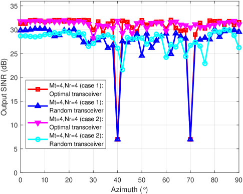
Figure 1: Relationship between output SINR and target angle with the directions of interferences being fixed.

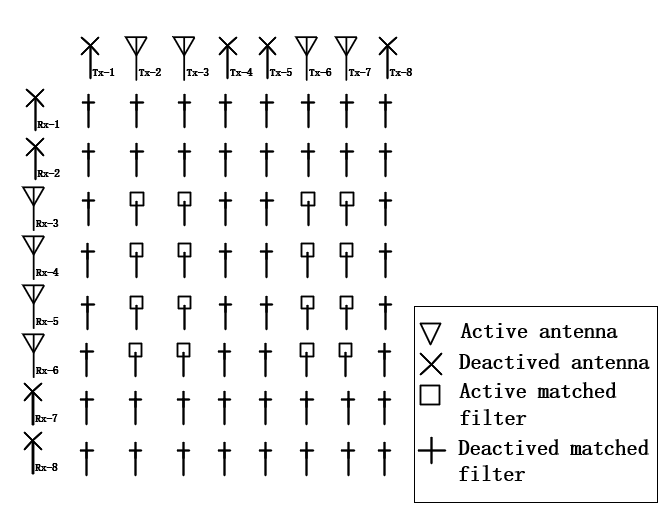
Figure 2: Optimal MIMO transceiver configuration when the target is from $80^{\circ}$.

Figure 3: Relationship between the output SINR and the target angle when the interferences are closed to the target.

V Conclusion

In this paper, the problem of sparse transceiver design for MIMO radar was considered. For a given number of transmitting and receiving sensors, a sparse MIMO array structure in terms of MaxSINR was jointly designed. A mixed-norm reweighted regularization was utilized to promote two-dimensional sparsity. It was shown by simulation examples that the proposed sparse MIMO transceiver selection algorithm provides superior interference suppression performance to randomly designed array.

References

- [1] M. G. Amin, X. Wang, Y. D. Zhang, F. Ahmad, and E. Aboutanios, “Sparse arrays and sampling for interference mitigation and DOA estimation in GNSS,” Proceedings of the IEEE, vol. 104, no. 6, pp. 1302–1317, June 2016.
- [2] A. Moffet, “Minimum-redundancy linear arrays,” IEEE Transactions on Antennas and Propagation, vol. 16, no. 2, pp. 172–175, March 1968.
- [3] P. Pal and P. P. Vaidyanathan, “Nested arrays: A novel approach to array processing with enhanced degrees of freedom,” IEEE Transactions on Signal Processing, vol. 58, no. 8, pp. 4167–4181, Aug. 2010.
- [4] M. G. Amin, P. P. Vaidyanathan, Y. D. Zhang, and P. Pal, “Editorial for coprime special issue,” Digital Signal Processing, vol. 61, no. Supplement C, pp. 1 – 2, 2017, special Issue on Coprime Sampling and Arrays.
- [5] S. Qin, Y. D. Zhang, and M. G. Amin, “Generalized coprime array configurations for direction-of-arrival estimation,” IEEE Transactions on Signal Processing, vol. 63, no. 6, pp. 1377–1390, March 2015.
- [6] A. Ahmed, Y. D. Zhang, and J. Zhang, “Coprime array design with minimum lag redundancy,” in ICASSP 2019 - 2019 IEEE International Conference on Acoustics, Speech and Signal Processing (ICASSP), May 2019, pp. 4125–4129.
- [7] M. H. Bae, I. H. Sohn, and S. B. Park, “Grating lobe reduction in ultrasonic synthetic focusing,” Electronics Letters, vol. 27, no. 14, pp. 1225–1227, July 1991.
- [8] J. Lu and J. Greenleaf, “Study of two-dimensional array transducers for limited diffraction beams,” IEEE Transactions on Ultrasonics, Ferroelectrics, and Frequency Control, vol. 41, no. 5, pp. 724–739, 9 1994.
- [9] J. H. Doles and F. D. Benedict, “Broad-band array design using the asymptotic theory of unequally spaced arrays,” IEEE Transactions on Antennas and Propagation, vol. 36, no. 1, pp. 27–33, Jan 1988.
- [10] V. Murino, A. Trucco, and A. Tesei, “Beam pattern formulation and analysis for wide-band beamforming systems using sparse arrays,” Signal Processing, vol. 56, no. 2, pp. 177 – 183, 1997.
- [11] X. Wang, C. P. Tan, F. Wu, and J. Wang, “Fault-tolerant attitude control for rigid spacecraft without angular velocity measurements,” IEEE Transactions on Cybernetics, pp. 1–14, 2019.
- [12] S. A. Hamza and M. G. Amin, “Sparse array beamforming design for wideband signal models,” IEEE Transactions on Aerospace and Electronic Systems, pp. 1–1, 2020.
- [13] X. Wang, M. G. Amin, and X. Wang, “Optimum sparse array design for multiple beamformers with common receiver,” in 2018 IEEE International Conference on Acoustics, Speech and Signal Processing, April 2018, pp. 4183–4186.
- [14] X. Wang, E. Aboutanios, M. Trinkle, and M. G. Amin, “Reconfigurable adaptive array beamforming by antenna selection,” IEEE Transactions on Signal Processing, vol. 62, no. 9, pp. 2385–2396, May 2014.
- [15] X. Wang, M. G. Amin, and X. Cao, “Optimum adaptive beamformer design with controlled quiescent pattern by antenna selection,” in 2017 IEEE Radar Conference (RadarConf), May 2017, pp. 0749–0754.
- [16] S. A. Hamza and M. G. Amin, “Optimum sparse array receive beamforming for wideband signal model,” in 2018 52nd Asilomar Conference on Signals, Systems, and Computers, Oct 2018, pp. 89–93.
- [17] S. A. Hamza and M. G. Amin, “Sparse array design utilizing matrix completion,” in 2019 Asilomar Conference on Signals, Systems, and Computers, Nov 2019.
- [18] S. A. Hamza, M. Amin, and G. Fabrizio, “Optimum sparse array design for maximizing signal-to-noise ratio in presence of local scatterings,” in 2018 IEEE International Conference on Acoustics, Speech and Signal Processing (ICASSP), April 2018.
- [19] X. Wang, M. Amin, and X. Cao, “Analysis and design of optimum sparse array configurations for adaptive beamforming,” IEEE Transactions on Signal Processing, vol. 66, no. 2, pp. 340–351, Jan 2018.
- [20] S. A. Hamza and M. G. Amin, “Hybrid sparse array design for under-determined models,” in ICASSP 2019 - 2019 IEEE International Conference on Acoustics, Speech and Signal Processing (ICASSP), May 2019, pp. 4180–4184.
- [21] ——, “Hybrid sparse array beamforming design for general rank signal models,” IEEE Transactions on Signal Processing, vol. 67, no. 24, pp. 6215–6226, Dec 2019.
- [22] W. Roberts, L. Xu, J. Li, and P. Stoica, “Sparse antenna array design for MIMO active sensing applications,” IEEE Transactions on Antennas and Propagation, vol. 59, no. 3, pp. 846–858, March 2011.
- [23] S. A. Hamza and M. G. Amin, “Sparse array design for transmit beamforming,” in 2020 IEEE Radar Conference, (submitted).
- [24] Z. Cheng, Y. Lu, Z. He, Yufengli, J. Li, and X. Luo, “Joint optimization of covariance matrix and antenna position for MIMO radar transmit beampattern matching design,” in 2018 IEEE Radar Conference (RadarConf18), April 2018, pp. 1073–1077.
- [25] S. A. Hamza and M. Amin, “Planar sparse array design for transmit beamforming (Conference Presentation),” in Radar Sensor Technology XXIV, K. I. Ranney and A. M. Raynal, Eds., vol. 11408, International Society for Optics and Photonics. SPIE, 2020. [Online]. Available: https://doi.org/10.1117/12.2557923
- [26] S. A. Hamza and M. G. Amin, “Sparse array design for transmit beamforming,” in 2020 IEEE International Radar Conference (RADAR), 2020, pp. 560–565.
- [27] S. Shahbazpanahi, A. B. Gershman, Z.-Q. Luo, and K. M. Wong, “Robust adaptive beamforming for general-rank signal models,” IEEE Transactions on Signal Processing, vol. 51, no. 9, pp. 2257–2269, Sept. 2003.
- [28] M. S. Ibrahim, A. Konar, M. Hong, and N. D. Sidiropoulos, “Mirror-prox sca algorithm for multicast beamforming and antenna selection,” 2018 IEEE 19th International Workshop on Signal Processing Advances in Wireless Communications (SPAWC), pp. 1–5, 2018.
- [29] E. J. Candès, M. B. Wakin, and S. P. Boyd, “Enhancing sparsity by reweighted minimization,” Journal of Fourier Analysis and Applications, vol. 14, no. 5, pp. 877–905, Dec. 2008.
- [30] X. Wang and E. Aboutanios, “Sparse array design for multiple switched beams using iterative antenna selection method,” Digital Signal Processing, vol. 105, p. 102684, 2020, special Issue on Optimum Sparse Arrays and Sensor Placement for Environmental Sensing.
- [31] O. Mehanna, N. D. Sidiropoulos, and G. B. Giannakis, “Joint multicast beamforming and antenna selection,” IEEE Transactions on Signal Processing, vol. 61, no. 10, pp. 2660–2674, May 2013.