ALMA: Alternating Minimization Algorithm For Clustering Mixture Multilayer Network

Abstract

The paper considers a Mixture Multilayer Stochastic Block Model (MMLSBM), where layers can be partitioned into groups of similar networks, and networks in each group are equipped with a distinct Stochastic Block Model. The goal is to partition the multilayer network into clusters of similar layers, and to identify communities in those layers. Jing et al. (2020) introduced the MMLSBM and developed a clustering methodology, TWIST, based on regularized tensor decomposition.

The present paper proposes a different technique, an alternating minimization algorithm (ALMA), that aims at simultaneous recovery of the layer partition, together with estimation of the matrices of connection probabilities of the distinct layers. Compared to TWIST, ALMA achieves higher accuracy, both theoretically and numerically.

Keywords: Stochastic Block Model, Multilayer Network, Alternating Minimization, Clustering

1 Introduction

Stochastic networks arise in many areas of research and applications and are used, for example, to study brain connectivity or gene regulatory mechanisms, to monitor cyber and homeland security, and to evaluate and predict social relationships within groups or between groups, such as countries.

While in the early years of the field of stochastic networks, research mainly focused on studying a single network, in recent years the frontier moved to investigation of collection of networks, the so called multilayer network, which allows to model relationships between nodes with respect to various modalities (e.g., relationships between species based on food or space), or consists of network data collected from different individuals (e.g., brain networks).

Although there are many different ways of modeling a multilayer network (see, e.g., an excellent review article of Kivela et al. (2014)), in this paper we consider the case where all layers have the same set of nodes, and all edges between nodes are drawn within layers, i.e., there are no edges connecting the nodes in different layers. MacDonald et al. (2021) called this type of networks the multiplex networks and argued that they appear in a variety of applications. Indeed, consider brain networks of several individuals that are drawn on the basis of some imaging modality. The nodes in the networks are associated with brain regions, and the brain regions are considered to be connected if the signals in those regions exhibit some kind of similarity. In this setting, the nodes are the same for each individual network, and there is no connection between brain regions of different individuals. For this reason, one can consider a multiplex network constituted by brain networks of several individuals, with common nodes but possibly different community structures in different layers (individuals). It is known that brain disorders are associated with changes in brain network organizations (see, e.g., Buckner and DiNicola (2019)), and that alterations in the community structure of the brain have been observed in several neuropsychiatric conditions, including Alzheimer disease (see, e.g., Chen et al. (2016)), schizophrenia (see, e.g., Stam (2014)) and epilepsy disease (see, e.g., Munsell et al. (2015)). Hence, assessment of the brain modular organization may provide a key to understanding the relation between aberrant connectivity and brain disease.

The multiplex networks have been studied by many authors who work in a variety of research fields. (see, e.g., Durante et al. (2017), Han and Dunson (2018), Aleta and Moreno (2019), Kao and Porter (2017) among others). In this paper, we consider a multilayer network where all layers are equipped with the Stochastic Block Models (SBM). In this case, the problems of interest include finding groups of layers that are similar in some sense, finding the communities in those groups of layers and estimation of the tensor of connection probabilities. While the scientific community attacked all three of those problems, often in a somewhat ad-hoc manner (see e.g., Brodka et al. (2018), Kao and Porter (2017), Mercado et al. (2018) among others), the theoretically inclined papers in the field of statistics mainly been investigated the case where communities persist throughout all layers of the network. This includes studying the so called “checker board model” in Chi et al. (2020), where the matrices of block probabilities take only finite number of values, and communities persist in all layers. The tensor block models of Wang and Zeng (2019) and Han et al. (2021) belong to the same category. In recent years, statistics publications extended this type of research to the case, where community structure persists but the matrix of probabilities of connections can take arbitrary values (see, e.g., Bhattacharyya and Chatterjee (2020), Paul and Chen (2020), Lei et al. (2019), Lei (2020), Paul and Chen (2016) and references therein). The authors studied precision of community detection and provided comparison between various techniques that can be employed in this case.

In many practical situations, however, the assumption of common community structures in all layers of the network may not be justified. Indeed, as we have stated above, some psychiatric or neurological conditions may be due to the alteration in the brain networks community structures rather than modifications in the strength of connections. For this reason, it is of interest to study a multiplex network with distinct community structures in groups of layers. Recently, Jing et al. (2020) investigated the so called “Mixture MultiLayer Stochastic Block Model” (MMLSBM), where there are $L$ layers can be partition into $M$ different types, with $M$ being a small number. In MMLSBM, each class $m$ of layers is equipped with its own community structure and a distinct matrix of connection probabilities $\boldsymbol{B}_{m}$, $m=1,...,M$. The methodology of Jing et al. (2020) is based on a regularized tensor decomposition, where all tensor dimensions are treated in the same way. The theory is developed under the assumption that the number of layers does not exceed the number of nodes. Note that the latter may not be true, for example, for brain networks, where the number of nodes is in hundreds (and is fixed) while the number of individuals, whose brain images are available, can grow indefinitely.

In this paper, we also consider the MMLSBM and suggest a new algorithm for the layer partition and local communities recovery. While the methodology of Jing et al. (2020) is based on a regularized tensor decomposition, our technique is centered around finding the groups of layers. Indeed, the “naive” approach to the problem would be to vectorize all adjacency matrices and cluster them using the k-means procedure. The major difference between our paper and Jing et al. (2020) is that we recognize that it is advantageous to treat within-layer and between-layer dimensions of the adjacency tensor in a different manner. Specifically, we propose a novel ALternating Minimization Algorithm (ALMA) which utilizes the fact that, for each layer of the network, the matrix of probabilities of connections can be approximated by a low-rank matrix. As a result, for the MMLSBM, our algorithm consistently recovers the layer labels and the memberships of nodes.

The present paper makes several contributions. First, it introduces the idea that the key to the inference in the MMLSBM is identification of the groups of layers: as soon as networks in each of $M$ layers are discovered, the communities can be found by the spectral algorithm of Lei and Rinaldo (2015), applied to the averages of the adjacency matrices. In addition, it uses the information that all layers are approximately low-rank. In comparison, the algorithm of Jing et al. (2020) only uses the information that the underlying tensor is approximately low-rank, which ignores the low-rankness within each layer. Due to this idea, as it follows from our theoretical analysis, ALMA achieves higher accuracy in the between-layer clustering. Also, as our numerical studies show, the latter leads to smaller between-layer and within-layer clustering errors, than for the algorithm of Jing et al. (2020). In addition, unlike the technique in Jing et al. (2020), ALMA does not require the assumption that the number of layers in the network is smaller than the number of nodes.

In this paper, we are not interested in the case of $M=1$, where communities are the same in all layers. Indeed, if one know that $M=1$, then, under the assumption that there are only $M=1$ types of matrices of connection probabilities, one can just find communities by spectral clustering after averaging. For this reason, one should not apply ALMA to the “checker board” or tensor block model, and ALMA should not be compared with techniques designed for this type of models.

Also, we assume that both the number of distinct layers $M$ and the number of communities in each group of layers are fixed and known in advance. While this is usually not true in practice, this is a very common assumption for theoretical investigations. When the algorithm is used in a real data setting, one needs to obtain solutions for several different values of $M$ and then choose the one that agrees with data. Since the probability tensor of the MMLSBM has sets of identical layers, we can borrow the idea from the problem of determining the number of clusters in a data set, when the $K$-means algorithm is used. One of the most popular heuristic methods is the so called “elbow method”. In our setting, we can run the algorithm with an increasing number of clusters $M$, and plot an error measure of the model as a function of $M$. This function would decrease as $M$ increases since models with larger $M$ explain more variations. Then, the elbow methods evaluate the curve of the function and find the “elbow of the curve”, i.e., the point where the function is no longer decreasing rapidly, as the number of distinct layers $M$ grow (see, e.g., Tibshirani et al. (2001), Zhang et al. (2012); Le and Levina (2015)). Other methods of choosing $M$ include cross-validation (Wang, 2010) and information criterion (Hu and Xu, 2003). After the number of groups of layers has been determined by one of the above mentioned techniques and the between-layers clustering has been implemented, one can identify the number of communities within each group of layers using common techniques employed in the Stochastic Block Models (SBMs) (Zhang et al., 2012; Le and Levina, 2015; Pensky and Zhang, 2019).

Note that dynamic network models can be viewed as a particular case of the multilayer network model where there are no edges connecting the nodes in different layers. The difference between those models and the multilayer network is that, in a dynamic network, the layers are ordered according to time instances, while in a multilayer network the enumeration of layers is completely arbitrary. That is why, although there is a multitude of papers that study the change point detection in the dynamic SBMs (see, e.g., Bhattacharjee et al. (2018), Gangrade et al. (2018) and Wang et al. (2017) among others), the techniques and error bounds in those papers are not applicable in the situation of the MMLSBM.

The rest of the paper is organized as follows. Section 2 describes the MMLSBM and presents the necessary concepts and notations. Section 3 introduces the Alternating Minimization Algorithm (ALMA). Section 4 provides theoretical guarantees for between-layer and within-layer clustering errors. Specifically, the section starts with Section 4.1 that investigates the situation where ALMA is applied to the true probability tensor. Based on the results of this analysis, Section 4.2 provides assumptions which, as it is confirmed in Section 4.3, guarantee convergence of our algorithm. Finally, Section 4.4 produces upper bounds for between-layer and within-layer clustering errors. Section 4 is concluded by a discussion of various aspects of ALMA in Section 4.5. Section 5 brings up theoretical and numerical comparisons between the ALMA and the TWIST algorithm, proposed in Jing et al. (2020). The proofs of all statements in the paper are deferred to Section 6, Appendix.

2 Model framework

This work considers an $L$-layer network on the same set of $n$ vertices ${\cal{V}}=\{1,\cdots,n\}$. For any $1\leq l\leq L$, the observed data is the adjacency matrix $\mathbf{A}_{l}\in\mathbb{R}^{n\times n}$ of the $l$-th network, where $\mathbf{A}_{l}(i,j)=\mathbf{A}_{l}(j,i)=1$ if a connection between nodes $i$ and $j$ is observed at the $l$-th network, and $\mathbf{A}_{l}(i,j)=\mathbf{A}_{l}(j,i)=0$ otherwise. Assume that for all $1\leq i<j\leq n$ and $1\leq l\leq L$, $\mathbf{A}_{l}(i,j)$ are the Bernoulli random variables with $\Pr(\mathbf{A}_{l}(i,j)=1)=\mathbf{P}_{*l}(i,j)$, and they are independent with each other. The probability matrices $\{\mathbf{P}_{*l}\}_{l=1}^{L}$ take $M$ different values ($M<L$), that is, there exists a partition of $[L]=\{1,\cdots,L\}=\cup_{m=1}^{M}{\mathcal{S}}_{m}$ such that $\mathbf{P}_{*l}=\tilde{\mathbf{Q}}_{*m}$ for all $l\in{\mathcal{S}}_{m}$. This means that there exists a clustering function $z:[L]\to[M]$ such that $z(l)=m$ if the $l$-th network is of the type $m$, or, equivalently, $l\in{\mathcal{S}}_{m}$. Consider a set ${\mathcal{F}}_{L,M}$ of the clustering matrices

$${\mathcal{F}}_{L,M}=\left\{\mathbf{Z}\in\{0,1\}^{L\times M},\quad\mathbf{Z}\mathbf{1}=\mathbf{1},\quad\mathbf{Z}^{T}\mathbf{1}\neq\mathbf{0}\right\},$$

and $\mathbf{Z}\in{\mathcal{F}}_{L,M}$ such that $\mathbf{Z}(l,m)=1$ if $l\in{\mathcal{S}}_{m}$ and $\mathbf{Z}(l,m)=0$ otherwise, and matrix $\mathbf{Z}$ does not have zero columns. It is easy to see that matrix $\mathbf{Z}^{T}\mathbf{Z}$ is diagonal, and $\mathbf{W}_{*}=\mathbf{Z}(\mathbf{Z}^{T}\mathbf{Z})^{-1/2}$ satisfies $\mathbf{W}_{*}^{T}\mathbf{W}_{*}=\mathbf{I}$. Here, $\mathbf{W}_{\star}(l,m)=L_{m}^{-1/2}$ if $l\in{\mathcal{S}}_{m}$ and $\mathbf{Z}(l,m)=0$ otherwise, where $L_{m}$ is the number of networks in the layer of type $m$, $m=1,...,M$.

Furthermore, we assume that each network can be described by a Stochastic Block Model (SBM). Specifically, we assume that, for each $m$ and any $l\in{\mathcal{S}}_{m}$, $\mathbf{P}_{*l}=\tilde{\mathbf{Q}}_{*m}$ where $\tilde{\mathbf{Q}}_{*m}$ is generated as follows: the nodes ${\cal{V}}$ are grouped into $K_{m}$ classes $G_{m,1},\cdots,G_{m,K_{m}}$, and the probability of a connection $\mathbf{P}_{*l}(i,j)$ is entirely determined by the groups to which the nodes $i$ and $j$ belong at $l$. In particular, if $i\in G_{m,k}$ and $j\in G_{m,k^{\prime}}$, then $\mathbf{P}_{*l}(i,j)=\mathbf{B}_{m}(k,k^{\prime})$, where $\mathbf{B}_{m}\in\mathbb{R}^{K_{m}\times K_{m}}$ is the connectivity matrix with $\mathbf{B}_{m}(k,k^{\prime})=\mathbf{B}_{m}(k^{\prime},k)$. In this case, one has

$$\mathbf{P}_{*l}=\mbox{$\Theta$}_{m}\mathbf{B}_{m}\mbox{$\Theta$}_{m}^{T},\quad m=z(l),\quad\mbox{$\Theta$}_{m}\in{\mathcal{F}}_{n,K_{m}},$$ (1)

where $\mbox{$\Theta$}_{m}(i,k)=1$ if and only if node $i$ belongs to the class $G_{m,k}$ and is zero otherwise.

Denote $\mathbf{Q}_{*m}=\sqrt{|{\mathcal{S}}_{m}|}\tilde{\mathbf{Q}}_{*m}$. Denote the three-way tensors with the $l$-th layer $\mathbf{A}_{l}$ and $\mathbf{P}_{*l}$ by, respectively, $\boldsymbol{A},\boldsymbol{P}_{*}\in\mathbb{R}^{L\times n\times n}$, and the three-way tensor with the $m$-th layer $\mathbf{Q}_{*m}$ by $\boldsymbol{Q}_{*}\in\mathbb{R}^{M\times n\times n}$.

The objective of this work is to partition the multilayer network ${\mathcal{A}}$ into $M$ similar layers (between-layer clustering) and, furthermore, for each of these sets of layers, to recover communities $G_{m,1},\cdots,G_{m,K_{m}}$, $m=1,\ldots,M$ (within layer clustering). Specifically, we focus on the setting where $M$ and $\{K_{m}\}_{m=1}^{M}$ are fixed or grow slowly, while $n$ and $L$ tend to infinity, since usually networks are large but have relatively few similar groups of layers, and the number of communities is also usually small compared to the number of nodes.

2.1 Notations

For any matrix $\mathbf{X}\in\mathbb{R}^{n_{1}\times n_{2}}$, denote the Frobenius and the operator norm of any matrix $\mathbf{X}$ by $\|\mathbf{X}\|_{F}$ and $\|\boldsymbol{X}\|$, respectively, and its $r$-th largest singular value by $\sigma_{r}(\mathbf{X})$. Let $\mbox{vec}(\mathbf{X})\in\mathbb{R}^{n_{1}n_{2}}$ be vectorization of matrix $\mathbf{X}$ obtained by sequentially stacking columns of matrix $\mathbf{X}$. Denote the projection operator onto the nearest orthogonal matrix by $\Pi_{o}$:

$$\Pi_{o}(\mathbf{X})=\mathbf{X}(\mathbf{X}^{T}\mathbf{X})^{-1/2}.$$ (2)

If $n_{1}\geq n_{2}$, then $\Pi_{o}(\mathbf{X})$ is an orthogonal matrix that has the same column space as $\mathbf{X}$. Specifically, if the singular value decomposition of $\mathbf{X}$ is $\mathbf{X}=\mathbf{U}\Sigma\mathbf{V}^{T}$, where $\mathbf{U}\in\mathbb{R}^{n_{1}\times n_{2}}$ and $\Sigma,\mathbf{V}\in\mathbb{R}^{n_{2}\times n_{2}}$, then $\Pi_{o}(\mathbf{X})=\mathbf{U}\mathbf{V}^{T}$.

For any tensor $\boldsymbol{X}\in\mathbb{R}^{n_{1}\times n_{2}\times n_{3}}$, its mode 1 matricization ${\mathcal{M}}_{1}(\boldsymbol{X})\in\mathbb{R}^{n_{1}\times n_{2}n_{3}}$ is a matrix such that $[{\mathcal{M}}_{1}(\boldsymbol{X})](l,:)=\mathrm{vec}(\boldsymbol{X}(l,:,:))$. For any tensor $\boldsymbol{X}\in\mathbb{R}^{n_{1}\times n_{2}\times n_{3}}$ and a matrix $\mathbf{A}\in\mathbb{R}^{m\times n_{1}}$, their mode-1 product $\boldsymbol{X}\times_{1}\mathbf{A}$ is a tensor in $\mathbb{R}^{m\times n_{2}\times n_{3}}$ defined by

$$[\boldsymbol{X}\times_{1}\mathbf{A}](j,i_{2},i_{3})=\sum_{i_{1}=1}^{n_{1}}\boldsymbol{X}(i_{1},i_{2},i_{3})\mathbf{A}(i_{1},j),\quad j=1,...,m.$$

In this product, every mode-1 fiber of tensor $\boldsymbol{X}$ is multiplied by matrix $\mathbf{A}$:

$$\mathbf{Y}=\mathbf{X}\times_{1}\mathbf{A}\Longleftrightarrow\widetilde{\mathbf{Y}}=\mathbf{A}\widetilde{\mathbf{X}},\quad\widetilde{\mathbf{Y}}={\mathcal{M}}_{1}(\mathbf{Y}),\ \widetilde{\mathbf{X}}={\mathcal{M}}_{1}(\mathbf{X})$$ (3)

If $\boldsymbol{X}\in\mathbb{R}^{n\times n_{2}\times n_{3}}$ and $\boldsymbol{Y}\in\mathbb{R}^{m\times n_{2}\times n_{3}}$ are two tensors, their mode-(2,3) product denoted by $\boldsymbol{X}\times_{2,3}\boldsymbol{Y}$, is a matrix in $\mathbb{R}^{n\times m}$ with elements $i_{1}=1,...,n$, $i_{2}=1,...,m$

$$[\boldsymbol{X}\times_{2,3}\boldsymbol{Y}](i_{1},i_{2})=\sum_{j_{2}=1}^{n_{2}}\sum_{j_{3}=1}^{n_{3}}\boldsymbol{X}(i_{1},j_{2},j_{3})\boldsymbol{Y}(i_{2},j_{2},j_{3})=\mbox{Tr}[X(i_{1},:,:)Y(i_{2},:,:)^{T}]$$

The Frobenius norm $\|\boldsymbol{X}\|_{F}$ and the largest singular value $\sigma_{1}(\boldsymbol{X})$ of a tensor $\boldsymbol{X}\in\mathbb{R}^{n_{1}\times n_{2}\times n_{3}}$ are defined by

$$\|\boldsymbol{X}\|_{F} =\sqrt{\sum_{i_{1},i_{2},i_{3}=1}^{n_{1},n_{2},n_{3}}\boldsymbol{X}(i_{1},i_{2},i_{3})^{2}},$$

$$\sigma_{1}(\boldsymbol{X})=\|\boldsymbol{X}\| =\max_{\mathbf{u}_{i}\in\mathbb{R}^{n_{i}},\|\mathbf{u}_{i}\|=1,1\leq i\leq 3}\boldsymbol{X}\times_{1}\mathbf{u}_{1}\times_{2}\mathbf{u}_{2}\times_{3}\mathbf{u}_{3}.$$

Operations above obey the following properties:
1. For $\mathbf{X}\in\mathbb{R}^{n_{1}\times n_{2}\times n_{3}}$, $\mathbf{A}\in\mathbb{R}^{m\times n_{1}}$, $\mathbf{Y}\in\mathbb{R}^{n\times n_{2}\times n_{3}}$ one has $(\mathbf{X}\times_{1}\mathbf{A})\times_{2,3}\mathbf{Y}=\mathbf{A}^{T}(\mathbf{X}\times_{2,3}\mathbf{Y})$
2.   If $\mathbf{W}$ is such that $\mathbf{W}^{T}\mathbf{W}=\mathbf{I}$, then $\|\mathbf{Q}\times_{1}\mathbf{W}^{T}\|^{2}_{F}=\|\mathbf{Q}\|^{2}_{F}$

For a more comprehensive tutorial for tensor algebra, please, see the review article of Kolda and Bader (2009).

Next, we introduce some notations that will be used later in the paper. Let $\mathbf{K}=(K_{1},\ldots,K_{M}),$ and denote

$$K_{\max}=\max_{m=1,\cdots,M}K_{m},\quad K_{\min}=\min_{m=1,\cdots,M}K_{m},\quad\dot{K}=\sum_{m=1}^{M}K_{m}.$$ (4)

Denote the size of the smallest cluster in all networks by $g_{\min}$, i.e., $\displaystyle{g_{\min}=\min_{\stackrel{{\scriptstyle 1\leq m\leq M}}{{1\leq k\leq K_{m}}}}\,|G_{m,k}|}$. Consider the SVDs of matrices $\boldsymbol{Q}_{*}(m,:,:)$ and the matrices $\Pi_{\mathbf{U}_{m}^{\perp}}$ orthogonal to the linear spaces of their eigenvectors:

$$\boldsymbol{Q}_{*}(m,:,:)=\mathbf{U}_{m}\mbox{$\Lambda$}_{m}\mathbf{U}_{m}^{T},\quad\Pi_{\mathbf{U}_{m}^{\perp}}=\mathbf{I}-\mathbf{U}_{m}\mathbf{U}_{m}^{T}$$ (5)

Since $\mathrm{rank}(\boldsymbol{Q}_{*}(m,:,:))=K_{m}$, $\mathbf{U}_{m}\in\mathbb{R}^{n\times K_{m}}$ is an orthogonal matrix that has the same column space as $\boldsymbol{Q}_{*}(m,:,:)$. Note that we somewhat abuse notations here: $\Pi_{\mathbf{U}_{m}^{\perp}}$ is a matrix and also an operator, so that, for any matrix $\mathbf{X}$, $\Pi_{\mathbf{U}_{m}^{\perp}}(\mathbf{X})$ is a projection of the matrix $\mathbf{X}$ on the linear space orthogonal to the column space of matrix $\mathbf{U}_{m}$.

Now, we introduce operators that will be used later in the paper. For any tensor $\boldsymbol{X}\in\mathbb{R}^{M\times n\times n}$, define a projector $\Pi_{\mathbf{K}}:\mathbb{R}^{M\times n\times n}\rightarrow\mathbb{R}^{M\times n\times n}$ by

$$[\Pi_{\mathbf{K}}(\boldsymbol{X})](m,:,:)=\Pi_{K_{m}}\big{(}\boldsymbol{X}(m,:,:)\big{)},\ m=1,\ldots,M,$$ (6)

where $\Pi_{K_{m}}:\mathbb{R}^{n\times n}\rightarrow\mathbb{R}^{n\times n}$ is the projection onto the nearest rank $K_{m}$ matrix. Consider operator $\Pi_{T,\mathbf{K}}:\mathbb{R}^{M\times n\times n}\to\mathbb{R}^{M\times n\times n}$ defined as

$$[\Pi_{T,\mathbf{K}}(\boldsymbol{X})](m,:,:) =\boldsymbol{X}(m,:,:)-\Pi_{\mathbf{U}_{m}^{\perp}}\boldsymbol{X}(m,:,:)\Pi_{\mathbf{U}_{m}^{\perp}},$$ (7)

where $\Pi_{\mathbf{U}_{m}^{\perp}}$ is defined in (5). In addition, let $\Pi_{T,K_{m}}:\mathbb{R}^{L\times n\times n}\rightarrow\mathbb{R}^{L\times n\times n}$ be the projection onto the subspace spanned by $\mathbf{U}_{m}$ for each “slice” of the tensor, i.e.,

$$[\Pi_{T,K_{m}}(\boldsymbol{X})](m^{\prime},:,:)=\boldsymbol{X}(m,:,:)-\Pi_{\mathbf{U}_{m}^{\perp}}\boldsymbol{X}(m,:,:)\Pi_{\mathbf{U}_{m}^{\perp}},\quad m^{\prime}=1,\ldots,M,$$

3 Alternating Minimization Algorithm (ALMA)

As we observe the multi-layer networks $\{\boldsymbol{A}_{l}\}_{l=1}^{L}$, our objectives are

• Between-layer clustering: recover the network classes ${\mathcal{S}}_{1},\cdots,{\mathcal{S}}_{M}$ such that $[L]=\cup_{m=1}^{M}{\mathcal{S}}_{m}$.

• Within-layer clustering: recover the community structures for each network class, i.e., for any $m\in[M]$, find a partition of the vertices $G_{m,1},\cdots,G_{m,K_{m}}$.

To achieve these goals, we start with the estimation of $\boldsymbol{Q}_{*}\in\mathbb{R}^{M\times n\times n}$ and $\mathbf{W}_{*}\in\mathbb{R}^{L\times M}$ based on $\boldsymbol{A}$. Then, the between-layer clustering can be carried out by applying $K$-means algorithm to the rows of the estimator $\widehat{\mathbf{W}}$ of matrix $\mathbf{W}_{*}$. Subsequently, the within-layer clustering of the $m$-th group of networks can be obtained by analyzing estimators $\hat{\boldsymbol{Q}}_{*}(m,:,:)$ of $\boldsymbol{Q}_{*}(m,:,:)$ for every $m\in[M]$.

In order to estimate $\boldsymbol{Q}_{*}$ and $\mathbf{W}_{*}$, note that the tensor $\boldsymbol{A}$ can be considered as a noisy observation of $\boldsymbol{P}_{*}$, since ${\mathbb{E}}(\boldsymbol{A})=\boldsymbol{P}_{*}$, where $\boldsymbol{P}_{*}=\boldsymbol{Q}_{*}\times_{1}\mathbf{W}_{*}^{T}$, and $\mathbf{W}_{*}$ is an orthogonal matrix by definition. For this reason, we propose to find $\boldsymbol{Q}_{*}$ and $\mathbf{W}_{*}$ by solving the following optimization problem

$$\underset{\boldsymbol{Q},\mathbf{W}}{\text{argmin}}\ \|\boldsymbol{A}-\boldsymbol{Q}\times_{1}\mathbf{W}^{T}\|_{F}$$ (8)

s.t. $$\boldsymbol{Q}\in\mathbb{R}^{M\times n\times n},\mathbf{W}\in\mathbb{R}^{L\times M} \mathbf{W}^{T}\mathbf{W}=\mathbf{I} \mathrm{rank}(\boldsymbol{Q}(m,:,:))\leq K_{m} 1\leq m\leq M$$, , for all .

We solve (8) by alternatively minimizing the objective function in (8) over $\mathbf{Q}$ and $\mathbf{W}$.

When $\mathbf{W}$ is fixed, the best approximation to $\boldsymbol{Q}$ is given by $\boldsymbol{Q}=\Pi_{\mathbf{K}}(\boldsymbol{A}\times_{1}\mathbf{W})$. Indeed, by equation (3), one has $\|\boldsymbol{A}-\boldsymbol{Q}\times_{1}\mathbf{W}\|_{F}=\|{\mathcal{M}}_{1}(\mathbf{A})-\mathbf{W}{\mathcal{M}}_{1}(\boldsymbol{Q})\|$. Hence, minimization of the last expression over $\boldsymbol{Q}$ yields ${\mathcal{M}}_{1}(\boldsymbol{Q})=\mathbf{W}^{T}{\mathcal{M}}_{1}(\mathbf{A})$ which, by (3), leads to $\boldsymbol{Q}=\mathbf{A}\times_{1}\mathbf{W}$. The latter, due to the rank restrictions, is approximated by the closest rank projection $\Pi_{\mathbf{K}}(\boldsymbol{A}\times_{1}\mathbf{W})$.

When $\boldsymbol{Q}$ is fixed, the problem of minimizing of $\|\boldsymbol{A}-\boldsymbol{Q}\times_{1}\mathbf{W}^{T}\|_{F}$ over $\mathbf{W}$ under the assumption that $\mathbf{W}^{T}\mathbf{W}=\mathbf{I}$, is called the orthogonal Procrustes problem (see, e.g., Gower and Dijksterhuis (2004)), and it has an explicit solution $\mathbf{W}=\Pi_{o}(\boldsymbol{A}\times_{2,3}\boldsymbol{Q})$, where $\Pi_{o}(\mathbf{X})$ is defined in (2). Combining the two steps, we summarize this alternating minimization procedure in Algorithm 1.

Algorithm 1 Alternating Minimization Algorithm (ALMA)

Input: Adjacency tensor $\boldsymbol{A}\in\mathbb{R}^{L\times n\times n}$; number of different types of networks $M$; $\{K_{m}\}_{m=1}^{M}$; Initialization clustering matrix $\mathbf{W}^{(1)}\in\mathbb{R}^{L\times M}$ such that $(\mathbf{W}^{(1)})^{T}\,\mathbf{W}^{(1)}=\mathbf{I}$

Output: A clustering matrix $\widehat{\mathbf{W}}\in\mathbb{R}^{L\times M}$ such that $\widehat{\mathbf{W}}^{T}\widehat{\mathbf{W}}=\mathbf{I}$, and a tensor $\widehat{\boldsymbol{Q}}\in\mathbb{R}^{M\times n\times n}$.

Steps:
1: Set $\mathrm{iter}=1$.

2: Let $\boldsymbol{Q}^{(\mathrm{iter}+1)}=\Pi_{\mathbf{K}}(\boldsymbol{A}\times_{1}\mathbf{W}^{(\mathrm{iter})})$, where $\Pi_{\mathbf{K}}$ is a projector defined in (6).

3: Let $\mathbf{W}^{(\mathrm{iter}+1)}=\Pi_{o}(\boldsymbol{A}\times_{2,3}\boldsymbol{Q}^{(\mathrm{iter}+1)})$ where $\Pi_{o}(\mathbf{X})$ is defined in (2).

4: Set $\mathrm{iter}=\mathrm{iter}+1$.

5: Repeat steps 2-4 until $\|\mathbf{W}^{(\mathrm{iter})}-\mathbf{W}^{(\mathrm{iter}-1)}\|_{F}\leq\epsilon_{n,L}$ where $\epsilon_{n,L}$ is a pre-specified threshold, or the number of iterations exceeds the upper limit: $\mathrm{iter}>N^{(iter)}$.

6: Set $\widehat{\mathbf{W}}=\mathbf{W}^{(\mathrm{iter}-1)}$, $\widehat{\boldsymbol{Q}}=\boldsymbol{Q}^{(\mathrm{iter}-1)}$.

After obtaining $\widehat{\mathbf{W}}$ and $\widehat{\boldsymbol{Q}}$, we recover the groups of similar networks ${\mathcal{S}}_{1},\cdots,{\mathcal{S}}_{M}$ by clustering the rows of $\widehat{\mathbf{W}}$ into $M$ groups using the $(1+\epsilon)$ approximate $K$-means algorithm. Finally, for clustering the nodes in each type of networks, we apply spectral clustering with $\widehat{\boldsymbol{Q}}(m,:,:)$ being treated as the affinity matrix. Specifically, we first find the orthogonal matrix of size $n\times K_{m}$ whose columns are the top $K_{m}$ eigenvectors of $\widehat{\boldsymbol{Q}}(m,:,:)$, and then cluster its rows into $K_{m}$ groups using the $(1+\epsilon)$ approximate $K$-means. There exist efficient algorithms for solving the $(1+\epsilon)$ approximate $K$-means problem, see, e.g., Kumar et al. (2004).

4 Theoretical guarantees

4.1 Convergence of the iterative algorithm for the true probability tensor

The purpose of this section is to explain how Algorithm 1 works. Indeed, in order this algorithm delivers acceptable solutions when it is applied the adjacency tensor $\mathbf{A}$, it should guarantee convergence when $\mathbf{A}$ is replaced by $\mathbf{P}_{*}$, and one starts from an arbitrary matrix $\mathbf{W}^{(1)}$. In this case, the associated optimization problem becomes

$$\underset{\boldsymbol{Q},\mathbf{W}}{\text{argmin}}\ \|\boldsymbol{P}_{*}-\boldsymbol{Q}\times_{1}\mathbf{W}^{T}\|_{F}$$ (9)

$$\text{s.t. $\boldsymbol{Q}\in\mathbb{R}^{M\times n\times n},\mathbf{W}\in\mathbb{R}^{L\times M}$, $\mathbf{W}^{T}\mathbf{W}=\mathbf{I}$, $\mathrm{rank}(\boldsymbol{Q}(m,:,:))\leq K_{m}$, for all $1\leq m\leq M$}.$$

Then, Algorithm 1 yields

$$\text{$\boldsymbol{Q}^{(\mathrm{iter})}=\Pi_{\mathbf{K}}(\boldsymbol{P}_{*}\times_{1}\mathbf{W}^{(\mathrm{iter}-1)})$,\ \ \ $\mathbf{W}^{(\mathrm{iter})}=\mathbf{W}_{*}\Pi_{o}(\boldsymbol{Q}_{*}\times_{2,3}\boldsymbol{Q}^{(\mathrm{iter})})$},$$ (10)

where the latter formula is obtained using $\boldsymbol{P}_{*}=\boldsymbol{Q}_{*}\times_{1}\mathbf{W}_{*}^{T}$. Hence,

$$\mathbf{W}^{(\mathrm{iter})}=\Pi_{o}(\boldsymbol{P}_{*}\times_{2,3}\boldsymbol{Q}^{(\mathrm{iter})})=\Pi_{o}(\mathbf{W}_{*}(\boldsymbol{Q}_{*}\times_{2,3}\boldsymbol{Q}^{(\mathrm{iter})}))=\mathbf{W}_{*}\Pi_{o}(\boldsymbol{Q}_{*}\times_{2,3}\boldsymbol{Q}^{(\mathrm{iter})}).$$

As a result, we can reformulate problem (9) by adding an assumption that $\mathbf{W}=\mathbf{W}_{*}\mathbf{V}$ for some $\mathbf{V}\in\mathbb{R}^{M\times M}$. Then (9) is simplified to

$$\underset{\boldsymbol{Q},\mathbf{V}}{\text{argmin}}\ \|\boldsymbol{Q}_{*}-\boldsymbol{Q}\times_{1}\mathbf{V}^{T}\|_{F}$$ (11)

s.t. $$\boldsymbol{Q}\in\mathbb{R}^{M\times n\times n},\mathbf{V}\in\mathbb{R}^{M\times M} \mathbf{V}^{T}\mathbf{V}=\mathbf{I} \mathrm{rank}(\boldsymbol{Q}(m,:,:))\leq K_{m} 1\leq m\leq M$$, , for all ,

and the iterative relations (10) become

$$\text{$\boldsymbol{Q}^{(\mathrm{iter})}=\Pi_{\mathbf{K}}(\boldsymbol{Q}_{*}\times_{1}\mathbf{V}^{(\mathrm{iter}-1)})$,\ \ \ $\mathbf{V}^{(\mathrm{iter})}=\Pi_{o}(\boldsymbol{Q}_{*}\times_{2,3}\boldsymbol{Q}^{(\mathrm{iter})})$},$$ (12)

where the first equation follows from the fact that

$$\boldsymbol{P}_{*}\times_{1}\mathbf{W}_{*}\mathbf{V}^{(\mathrm{iter}-1)}=(\boldsymbol{P}_{*}\times_{1}\mathbf{W}_{*})\times_{1}\mathbf{V}^{(\mathrm{iter}-1)}=\boldsymbol{Q}_{*}\times_{1}\mathbf{V}^{(\mathrm{iter}-1)}.$$

The latter implies that, for the sets ${\mathcal{S}}_{1}$ and ${\mathcal{S}}_{2}$ in $\mathbb{R}^{M\times n\times n}$ defined by

$${\mathcal{S}}_{1} =\{\boldsymbol{Q}:\mathrm{rank}(\boldsymbol{Q}(m,:,:))\leq K_{m}\ \mbox{for all}\ 1\leq m\leq M\},$$

$${\mathcal{S}}_{2} =\{\boldsymbol{Q}=\boldsymbol{Q}_{*}\times_{1}\mathbf{V}:\mathbf{V}\in\mathbb{R}^{M\times M},\mathbf{V}^{T}\mathbf{V}=\mathbf{I}\},$$

$\boldsymbol{Q}^{(\mathrm{iter})}$ is the nearest point on ${\mathcal{S}}_{1}$ to $\boldsymbol{Q}_{*}\times_{1}\mathbf{V}^{(\mathrm{iter}-1)}$, and $\boldsymbol{Q}_{*}\times_{2,3}\mathbf{V}^{(\mathrm{iter})}$ is the nearest point on ${\mathcal{S}}_{2}$ to $\boldsymbol{Q}^{(\mathrm{iter})}$. Hence, the update formula (12) can be viewed as an alternating projection between ${\mathcal{S}}_{1}$ and ${\mathcal{S}}_{2}$.

Denote the tangent planes to the sets ${\mathcal{S}}_{1}$ and ${\mathcal{S}}_{2}$ at $\boldsymbol{Q}_{*}$ by $L_{1}$ and $L_{2}$, respectively. Then, the explicit formulas for $L_{1}$ and $L_{2}$ are given by

$$L_{1} =\{\boldsymbol{Q}\in\mathbb{R}^{M\times n\times n}:\Pi_{\mathbf{U}_{m}^{\perp}}\boldsymbol{Q}(m,:,:)\Pi_{\mathbf{U}_{m}^{\perp}}=\mathbf{0},\quad m=1,\ldots,M,\}$$ (13)

$$L_{2} =\{\boldsymbol{Q}=\boldsymbol{Q}_{*}\times_{1}\mathbf{X}:\mathbf{X}\in\mathrm{Skew}_{M}\},$$

where $\mathrm{Skew}_{M}$ represents the set of skew-symmetric matrices of size $M\times M$. The intuition, the formal definition of tangent space, and the derivations of $L_{1}$ and $L_{2}$ are deferred to Section 6.1.

Hence, the “alternating projection” viewpoint of (12) reveals that it is approximately an alternating projection procedure between the subspaces $L_{1}$ and $L_{2}$. Since the projections onto $L_{1}$ and $L_{2}$ are linear operators, the convergence rate of this alternating projection method can be described by the operator norm of the composite operator:

$$\kappa_{H}=\max_{\boldsymbol{X}\in\mathbb{R}^{M\times n\times n}}\frac{\|P_{L_{2}}P_{L_{1}}\boldsymbol{X}\|_{F}}{\|\boldsymbol{X}\|_{F}}.$$ (14)

Since $P_{L_{1}}$ and $P_{L_{2}}$ are projection operators, one has $\|P_{L_{1}}(\boldsymbol{X})\|_{F}\leq\|\boldsymbol{X}\|_{F}$, $\|P_{L_{2}}(\boldsymbol{X})\|_{F}\leq\|\boldsymbol{X}\|_{F}$ and, therefore, $\kappa_{H}\leq 1$.

Note that $\kappa_{H}$ can be expressed via the smallest principal angle $\theta$ between planes $L_{1}$ and $L_{2}$: $\kappa_{H}=\cos(\theta)$. In particular, $\kappa_{H}=0$ if $L_{1}$ and $L_{2}$ are perpendicular to each other, and $\kappa_{H}=1$ if intersection $L_{1}\cap L_{2}$ is nontrivial. As an example, when $M=2$, one has $\dim(L_{2})=1$, and $\kappa_{H}$ can be explicitly written as

$$\kappa_{H}=\sqrt{\frac{{\|\boldsymbol{Q}_{*}(1,:,:)-\Pi_{\mathbf{U}_{2}^{\perp}}\boldsymbol{Q}_{*}(1,:,:)\Pi_{\mathbf{U}_{2}^{\perp}}\|_{F}^{2}}+\|\boldsymbol{Q}_{*}(2,:,:)-\Pi_{\mathbf{U}_{1}^{\perp}}\boldsymbol{Q}_{*}(2,:,:)\Pi_{\mathbf{U}_{1}^{\perp}}\|_{F}^{2}}{{\|\boldsymbol{Q}_{*}(1,:,:)\|_{F}^{2}+\|\boldsymbol{Q}_{*}(2,:,:)\|_{F}^{2}}}}.$$

Since the algorithm in (12) is approximately an alternating projection procedure between the subspaces $L_{1}$ and $L_{2}$, it converges faster for smaller values of $\kappa_{H}$. Note that $\kappa_{H}=1$ if and only if $P_{L_{2}}P_{L_{1}}\boldsymbol{X}=\boldsymbol{X}$ for some $\boldsymbol{X}$, i.e., when there is a nontrivial intersection between planes $L_{1}$ and $L_{2}$.

4.2 Assumptions

In order to guarantee linear convergence of Algorithm 1 when it is applied to the true probability tensor $\mathbf{P}_{*}$, we make the following assumption:

(A1). The subspaces $L_{1}$ and $L_{2}$, defined in (13), have only trivial intersection at the origin.

While Assumption (A1) is somewhat complicated, it is actually not very restrictive. Specifically, the statement below provides two very simple sufficient conditions that guarantee Assumption (A1). In particular, Assumption (A1(b)) holds if each clustering pattern is not obtained by mixing other clustering patterns via combining or intersecting the clusters. For example, Assumption (A1(b)) holds with high probability when the $M$ clustering patterns are drawn uniformly at random.

Lemma 1.

Let at least one of the following conditions hold:

(A1(a)). For every $1\leq m\leq M$, the sets of $(M-1)$ matrices

$$\left\{\Pi_{\mathbf{U}_{m}^{\perp}}\boldsymbol{Q}_{*}(m^{\prime},:,:)\Pi_{\mathbf{U}_{m}^{\perp}},m^{\prime}\neq m,1\leq m^{\prime}\leq M\right\}$$

are linearly independent. That is, the vectorized versions of those matrices, a matrix of size $n^{2}\times M$ with the m-th column given by $\mbox{vec}(\Pi_{\mathbf{U}_{m}^{\perp}}\boldsymbol{Q}_{*}(m^{\prime},:,:)\Pi_{\mathbf{U}_{m}^{\perp}})$, has rank $(M-1)$.

(A1(b)). For all $1\leq m\leq M$, one has

$$\mbox{Span}(\mbox{$\Theta$}_{m})\not\in\bigoplus_{1\leq m^{\prime}\leq M,m^{\prime}\neq m}\mbox{Span}(\mbox{$\Theta$}_{m^{\prime}}),$$

where $\mbox{$\Theta$}_{m}\in\mathbb{R}^{n\times K_{m}}$ is the membership matrix for the $m$-th network as defined in (1) and $\oplus$ stands for the direct sum of subspaces.

The proof that these conditions are sufficient is presented in Section 6.5. While conditions in Lemma 1 are sufficient, they are not necessary. A more detailed discussion of assumption (A1) is deferred to Section 4.5.1.

In addition, we impose few other natural assumptions as follows:

(A2). There exist absolute constants $c_{0}>0$ such that $K_{\max}M\leq c_{0}\dot{K}$, where $\dot{K}$ is defined in (4).

(A3). The layers in the network, as well as local communities in each network are balanced, i.e., there exist absolute constants $c_{1},c_{2},c_{3},c_{4}$ such that

$$c_{1}\,\frac{L}{M}\leq L_{m}\leq c_{2}\,\frac{L}{M},\quad c_{3}\,\frac{n}{K_{m}}\leq|G_{m,k}|\leq c_{4}\,\frac{n}{K_{m}}\quad\mbox{for any}\ \ 1\leq m\leq M,\ 1\leq k\leq K_{m},$$ (15)

where $|G_{m,k}|$ is the size of the $k$-th community in cluster $m$.

(A4). There exist matrices $\mathbf{B}^{0}_{m}\in\mathbb{R}^{K_{m}\times K_{m}}$, $m=1,\ldots,M$, such that $\mathbf{B}_{m}=p_{\max}\mathbf{B}^{0}_{m}$, where $p_{\max}\in(0,1]$ controls the overall network sparsity and the matrices $\mathbf{B}^{0}_{m}$ are such that, for all $m=1,...,M$, there exists some absolute constants $b_{1}>0$ and $b_{2}>0$ such that

$$\sigma_{K_{m}}(\mathbf{B}_{m}^{0})\geq b_{1},\quad\|\mathbf{B}_{m}^{0}\|_{F}\geq b_{2}\,K_{m},\quad\|\mathbf{B}_{m}^{0}\|_{\infty}\leq 1.$$ (16)

We remark that the first two inequalities of (16) imply that the magnitude of $\mathbf{B}_{m}^{0}$ is bounded from below, while the last inequality of (16) ensures that the magnitude of $\mathbf{B}_{m}^{0}$ is bounded from above. In addition, $\|\mathbf{B}_{m}^{0}\|_{\infty}\geq K_{m}^{-1}\,\|\mathbf{B}_{m}^{0}\|_{F}$, and (16) guarantees that $\|\mathbf{B}_{m}^{0}\|_{\infty}$ is bounded from both below and above: $b_{2}\leq\|\mathbf{B}_{m}^{0}\|_{\infty}\leq 1$.

4.3 Convergence of ALMA

Denote by $\kappa_{0}$ the condition number of matrix $\boldsymbol{Q}_{*}\times_{2,3}\boldsymbol{Q}_{*}$:

$$\kappa_{0}=\frac{\sigma_{1}(\boldsymbol{Q}_{*}\times_{2,3}\boldsymbol{Q}_{*})}{\sigma_{M}(\boldsymbol{Q}_{*}\times_{2,3}\boldsymbol{Q}_{*})}.$$

Let

$$\beta_{n,L}=\log^{2}(n+L)\sqrt{M^{3}\,\kappa_{0}^{5}}\left(\sqrt{\frac{1}{p_{\max}n^{2}}}+\frac{\dot{K}^{2}}{p_{\max}n\min(n,L)}\right)$$ (17)

Then, the following theorem shows that, with a good initialization that satisfies (19), as the number of iterations tends to infinity, Algorithm 1 converges to a fixed point that is close to $\boldsymbol{Q}_{*}$ and $\mathbf{W}_{*}$.

Theorem 1.

Let Assumptions (A1)-(A4) hold and $\kappa_{H}$ be uniformly bounded away from one for any $n$ and $L$ large enough. Let, for some positive absolute constant $C_{1}$

$$p_{\max}\,\geq C_{1}\max\left(\frac{\kappa_{0}^{12}\log^{6}(n+L)M^{3}\dot{K}^{3}}{(1-\kappa_{H})^{4}\,n\,\min(n,L)},\frac{\log(n+L)}{n+L}\right)$$ (18)

and the initialization $\mathbf{W}^{(1)}$ has an estimation error bounded above by some positive function $h$ of $M,\dot{K}$ and $\kappa_{0}$:

$$\|\mathbf{W}^{(1)}-\mathbf{W}_{*}\|_{F}\leq h(M,\dot{K},\kappa_{0}).$$ (19)

Then, for some absolute constant $C_{2}>0$ and $\mathrm{iter}\geq 1$, with probability $1-o(1)$ as $n,L\rightarrow\infty$, one has

$$\|{\mathbf{W}}^{(\mathrm{iter}+1)}-\mathbf{W}_{*}\|_{F}\leq\frac{1+\kappa_{H}}{2}\|{\mathbf{W}}^{(\mathrm{iter})}-\mathbf{W}_{*}\|_{F}+{C_{2}}\,\beta_{n,L}$$ (20)

Moreover, for any $\mathrm{iter}>1$, one has

$$\|{\mathbf{W}}^{(\mathrm{iter})}-\mathbf{W}_{*}\|_{F}\leq\left(\frac{1+\kappa_{H}}{2}\right)^{\mathrm{iter}-1}\,\|{\mathbf{W}}^{(1)}-\mathbf{W}_{*}\|_{F}+\frac{2C_{2}}{1-\kappa_{H}}\,\beta_{n,L},$$

with probability $1-o(1)$ as $n,L\rightarrow\infty$. Consequently, if $\displaystyle\widetilde{\mathbf{W}}=\lim_{\mathrm{iter}\rightarrow\infty}{\mathbf{W}}^{(\mathrm{iter})}$ and $\displaystyle\widetilde{\boldsymbol{Q}}=\lim_{\mathrm{iter}\rightarrow\infty}{\boldsymbol{Q}}^{(\mathrm{iter})}$, then

$$\|\widetilde{\mathbf{W}}-\mathbf{W}_{*}\|_{F}\leq\frac{2C_{2}}{1-\kappa_{H}}\,\beta_{n,L}$$ (21)

In addition, with probability $1-o(1)$ as $n,L\rightarrow\infty$, for some absolute constant $C_{3}>0$ and any $m=1,\ldots,M$, one has

$$\left\|[\boldsymbol{Q}^{(\mathrm{iter})}-\boldsymbol{Q}_{*}](m,:,:)\right\|\leq 2p_{\max}\,n\,\sqrt{L}\|{\mathbf{W}}^{(\mathrm{iter})}-\mathbf{W}_{*}\|_{F}+C_{3}\,\sqrt{p_{\max}(n+L)}\,\log(n+L).$$ (22)

Based on the iterative update formula for the estimation error in (20), we can assess performance of Algorithm 1 with the stopping criterion $\epsilon_{n,L}$.

Corollary 1.

Under the assumptions and the notations of Theorem 1, if

$$\|{\mathbf{W}}^{(\mathrm{iter}+1)}-{\mathbf{W}}^{(\mathrm{iter})}\|_{F}\leq\epsilon_{n,L},$$ (23)

then, with probability $1-o(1)$ as $n,L\rightarrow\infty$, one has

$$\|{\mathbf{W}}^{(\mathrm{iter})}-\mathbf{W}_{*}\|_{F}\leq\frac{2\epsilon_{n,L}}{1-\kappa_{H}}\,+\frac{2C_{2}}{1-\kappa_{H}}\,\beta_{n,L}.$$ (24)

As a result, if $\epsilon_{n,L}\geq 6\,C_{2}\,(1-\kappa_{H})^{-1}\,\beta_{n,L}$, then Algorithm 1 would stop within at most $T_{n,L}$ iterations, where

$$T_{n,L}=\log\left(\frac{6\,\|\mathbf{W}^{(1)}-\mathbf{W}_{*}\|_{F}}{\epsilon_{n,L}}\right)\Bigg{/}\log\left(\frac{2}{1+\kappa_{H}}\right)$$

Remark 1.

Permutations.   We remark that $\mathbf{W}^{(1)}$ needs to be close to $\mathbf{W}_{*}$ up to a permutation of columns, but this permutation has no impact on the between-layer and within-layer clustering results, as the outputs of Algorithm 1, $\widehat{\mathbf{W}}$ and $\widehat{\boldsymbol{Q}}$, would also be close to $\mathbf{W}_{*}$ and $\boldsymbol{Q}_{*}$ up to permutations of columns and layers, respectively.

Remark 2.

Initialization.   Theorem 1 and Corollary 1 require initialization $\mathbf{W}^{(1)}$ that satisfies condition (19). If $M$, $\dot{K}$ and $\kappa_{0}$ are uniformly bounded above for any values of $n$ and $L$, then (19) is satisfied by any matrix $\mathbf{W}^{(1)}$ since for any $L\times M$ matrix $\mathbf{W}$ such that $\mathbf{W}^{T}\mathbf{W}=I_{M}$ one has $\|\mathbf{W}\|^{2}_{F}=M$, i.e. condition (19) holds with $h(M,\dot{K},\kappa_{0})=2\sqrt{M}$. In order to obtain more precise results, one can first obtain an initial between-layer clustering matrix $\mathbf{Z}^{(1)}\in\{0,1\}^{L\times M}$ using, e.g., spectral clustering algorithm on vectorized layer matrices $\{\mathbf{A}_{l}\}_{l=1}^{L}$, and then set

$${\mathbf{W}}^{(1)}=\mathbf{Z}^{(1)}((\mathbf{Z}^{(1)})^{T}\mathbf{Z}^{(1)})^{-1/2}.$$ (25)

However, as it follows from Theorem 1 and Corollary 1, the errors are smaller and the convergence of ALMA algorithm is faster when a more accurate initialization $\mathbf{W}^{(1)}$ is used. For this reason, in Section 4.5.2 we present a more involved initialization procedure.

Sketch of the proof.   The proof of Theorem 1 is deferred to Section 6.2. Below we provide some insight into how this theorem can be proved. The proof of the main inequality (20) in Theorem 1 can be divided into four steps.

The first step establishes a deterministic bound on $\|{\mathbf{W}}^{(\mathrm{iter})}-\mathbf{W}_{*}\|$ for any given fixed $\boldsymbol{A}$. The second and the third steps establish probabilistic bounds for a random tensor $\boldsymbol{A}$ under the probabilistic model in Section 2. Finally, the fourth step simplifies this probabilistic bound using Assumptions (A2)-(A4).

As for the proof of (22), it is based on the following chain of inequalities

$$\|[\hat{\boldsymbol{Q}}-\boldsymbol{Q}_{*}](m,:,:)\| =\|\Pi_{K_{m}}[\boldsymbol{A}\times_{1}\hat{\mathbf{W}}]-\boldsymbol{Q}_{*}(m,:,:)\|\leq 2\|\boldsymbol{A}\times_{1}\hat{\mathbf{W}}-\boldsymbol{Q}_{*}(m,:,:)\|$$

$$\leq 2\|\boldsymbol{P}_{*}\times_{1}(\hat{\mathbf{W}}-\mathbf{W}_{*})\|+2\|\boldsymbol{\Delta}\times_{1}\hat{\mathbf{W}}(:,m)\|\leq 2\|\boldsymbol{Q}_{*}\|\|\hat{\mathbf{W}}-\mathbf{W}_{*}\|+2\|\boldsymbol{\Delta}\|$$

$$\leq 2\|\boldsymbol{Q}_{*}\|\|\hat{\mathbf{W}}-\mathbf{W}_{*}\|_{F}+2\|\boldsymbol{\Delta}\|,$$ (26)

where $\boldsymbol{\Delta}=\boldsymbol{A}-\boldsymbol{P}_{*}$, and the factor 2 in the first inequality follows from

$$\|\boldsymbol{A}\times_{1}\hat{\mathbf{W}}-\Pi_{K_{m}}[\boldsymbol{A}\times_{1}\hat{\mathbf{W}}]\|\leq\|\boldsymbol{A}\times_{1}\hat{\mathbf{W}}-\boldsymbol{Q}_{*}(m,:,:)\|.$$

Inequality (22) is then obtained by combining (26) with the upper bounds on $\|\boldsymbol{\Delta}\|$ in Lemma 3 (see Appendix) and the fact that $\|\boldsymbol{Q}_{*}\|\leq\|\boldsymbol{Q}_{*}\|_{F}\leq p_{\max}n\sqrt{L}$.

4.4 Consistency of between-layer and within-layer clustering

This section studies misclassification error rates of network clustering and local community detection. The misclassification error rates are measured by the Hamming distance between clustering partitions. Since the clustering is unique only up to a permutation of clusters, denote the set of permutation functions of $[r]=\{1,\cdots,r\}$ by $\aleph(r)$.

Given the true partition of network layers $[L]=\{1,\cdots,L\}=\cup_{m=1}^{M}{\mathcal{S}}_{m}$ and the estimated partition $[L]=\cup_{m=1}^{M}\hat{{\mathcal{S}}}_{m}$, the misclassification error rate of between-layer clustering is given by

$${R_{BL}=L^{-1}\ \min_{\tau\in\aleph{(M)}}\ \sum_{m=1}^{M}|{\mathcal{S}}_{m}\setminus\hat{{\mathcal{S}}}_{\tau(m)}|.}$$ (27)

The misclassification rate of within-layer clustering is defined similarly: given the true partition of vertices $[n]=\{1,\cdots,n\}=\cup_{k=1}^{K_{m}}G_{m,k}$ and the estimated partition $\cup_{k=1}^{K_{m}}\hat{G}_{m,k}$, the misclassification error rate of within-layer clustering for the $m$-th group of layers is given by

$${R_{WL}(m)=n^{-1}\ \min_{\tau\in\aleph(K_{m})}\ \sum_{k=1}^{K_{m}}|G_{m,k}\setminus\hat{G}_{m,\tau(k)}|.}$$ (28)

The derivations of both misclassification rates are based on the upper bound (22) and Lemma C.1 of Lei (2020). In addition, the analysis of within-layer clustering also applies the Davis-Kahan theorem. Our results on the misclassification errors are as follows, with the proof deferred to Section 6.3.

Theorem 2.

(a) [Between-layer clustering error] For an $(1+\epsilon)$ approximate solution of the $K$-means problem, with probability $1-o(1)$ as $n,L\rightarrow\infty$, the between-layer clustering error is bounded by

$$R_{BL}\leq C_{\epsilon}\,\frac{\beta_{n,L}^{2}}{M^{2}(1-\kappa_{H})^{2}}.$$ (29)

for some constant $C_{\epsilon}$ depending on $\epsilon$.

(b) [Within-layer clustering] With probability $1-o(1)$ as $n,L\rightarrow\infty$, the within-layer clustering error of the $m$-th type of network is bounded by

$$R_{WL}(m)\leq C_{\epsilon}K_{\max}\left(\frac{\beta_{n,L}^{2}}{(1-\kappa_{H})^{2}}+\frac{\log^{2}(n+L)}{n\,L\,p_{\max}}\right),\quad m=1,\ldots,M.$$ (30)

Here, $\kappa_{H}$ and $\beta_{n,L}$ are defined in, respectively, (14) and (17).

4.5 Discussion of theoretical guarantees

4.5.1 Discussion of Assumption (A1)

This section shows that Assumption (A1) is not restrictive, and is usually satisfied in practice. In Lemma 1, we have already provided sufficient conditions that guarantee validity of Assumption (A1). Below, we continue the discussion of this assumption.

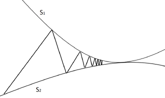
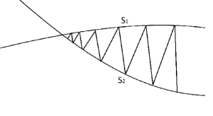
Figure 1: Examples of convergence rates of the alternating projection algorithm. Left: ${\mathcal{S}}_{1}$ and ${\mathcal{S}}_{2}$ are “tangent” to each other and their tangent planes have nontrivial intersections. Right: the tangent planes of ${\mathcal{S}}_{1}$ and ${\mathcal{S}}_{2}$ only have a trivial intersection.

The fact that Assumption (A1) is not restrictive can also be inferred from counting the dimensions of $L_{1}$ and $L_{2}$. Since a symmetric matrix $\boldsymbol{Q}(m,:,:)$ has $n(n-1)/2$ degrees of freedom, the set

$$\{\boldsymbol{Q}(m,:,:):\Pi_{\mathbf{U}_{m}^{\perp}}\boldsymbol{Q}_{(}m,:,:)\Pi_{\mathbf{U}_{m}^{\perp}}=\mathbf{0}\}$$

has $n(n-1)/2-(n-K_{m})(n-K_{m}-1)/2=K_{m}n-K_{m}(K_{m}+1)/2$ degrees of freedom. Summing those up for $1\leq m\leq M$, obtain that the dimension of $L_{1}$ is $\sum_{m=1}^{M}(K_{m}n-K_{m}(K_{m}+1)/2)$. Since the set $\mathrm{Skew}_{M}$ has $M(M-1)/2$ degrees of freedom, $L_{2}$ has a dimension of $M(M-1)/2$. Since random subspaces of dimensions $d_{1}$ and $d_{2}$ in $\mathbb{R}^{D}$ do not intersect if $d_{1}+d_{2}\leq D$, that is, if

$$\frac{M(M-1)}{2}+\sum_{m=1}^{M}(K_{m}n-\frac{K_{m}(K_{m}+1)}{2})\leq M\,n^{2},$$

(which holds when $n$ is large), then (A1(b)) should usually hold.

We also remark that Assumption (A1) is slightly more restrictive than the local uniqueness of the solution to the problem (8) in the noiseless scenario, which only requires that ${\mathcal{S}}_{1}$ and ${\mathcal{S}}_{2}$ intersect only at $\boldsymbol{Q}_{*}$. However, our goal is to prove the linear convergence of Algorithm 1, and, as it is shown in Figure 1 below, the convergence rate of the alternating method in Algorithm 1 would be slow and nonlinear if ${\mathcal{S}}_{1}$ and ${\mathcal{S}}_{2}$ are “tangent” to each other and their tangent planes have nontrivial intersections. On the other hand, the convergence rate is linear if the tangent planes to ${\mathcal{S}}_{1}$ and ${\mathcal{S}}_{2}$ have only a trivial intersection.

We should mention that Assumption (A1) fails in the case of the “checker board” model of Chi et al. (2020), where all networks have the same community structures. As we have indicated, we are not interested in carrying out the inference in this case. However, we remark that the ALMA still succeeds empirically in the checker board model, even though the Assumption (A1) is violated.

Remark 3.

Uniqueness of the solution.   Similar to many clustering problems, the solution of the optimization problem (9) is unique only up to permutations of clusters. The non-uniqueness due to permutation of clusters, however, does not cause difficulty for Algorithm 1. Hence, Theorem 1 still applies: if the initialization $\mathbf{W}^{(1)}$ is reasonably close to $\mathbf{W}_{*}$, then Algorithm 1 converges to the true solution.

4.5.2 Initialization

We remark that Theorem 1 and Corollary 1 require a good initialization such that (19) holds. Also, as Remark 2 states, the errors in Theorem 1 and Corollary 1 are smaller, and the convergence of Algorithm 1 is faster when a more accurate initialization $\mathbf{W}^{(1)}$ is used. For this reason, in this section we present a more involved initialization procedure, summarized in Algorithm 2, which is based on an initial estimator of the between-layer clustering.

Algorithm 2 Initialization of Algorithm 1

Input: Adjacency matrices $\mathbf{A}_{l}\in\mathbb{R}^{n\times n}$, $1\leq l\leq L$; number of different layers $M$; $\dot{K}$.

Output: $\mathbf{W}^{(1)}$.

Steps:
1: Set $\mathbf{W}^{(0)}\in\mathbb{R}^{L\times M}$ to be composed of the top $M$ left singular vectors of ${\mathcal{M}}_{3}(\boldsymbol{A})$.

2: Apply the $K$-means algorithms to the rows of $\mathbf{W}^{(0)}$ to obtain an initial estimator of the between-layer clustering $[L]=\cup_{m=1}^{M}\tilde{{\mathcal{S}}}_{m}$.

3: Apply (25) to obtain $\mathbf{W}^{(1)}$ from $[L]=\cup_{m=1}^{M}\tilde{{\mathcal{S}}}_{m}$.

Theoretical guarantees on this initialization are given by the statement below. Its proof is deferred to Section 6.5.

Proposition 1.

(Theoretical guarantee of Algorithm 2.)  Assume that $p_{\max}\geq c\frac{\log(n^{2}+L)}{\min(n^{2},L)}$ for some constant $c>0$. Then for any $r>0$, there exists a constant $C>0$ depending only on $r,c,k$, such that, with probability at least $1-n^{-r}$ ,

$$\|\mathbf{W}^{(1)}-\mathbf{W}_{*}\|_{F}\leq\sqrt{\frac{C_{\epsilon}M(n^{2}+L)}{p_{\max}n^{2}L}}\ \frac{\displaystyle\max_{1\leq m\leq M}L_{m}}{\displaystyle\min_{1\leq m\leq M}L_{m}}.$$

Let us discuss Proposition 1 under the assumptions that $M,\dot{K},\kappa_{0}$ and $\frac{\max_{1\leq m\leq M}L_{m}}{\min_{1\leq m\leq M}L_{m}}$ are uniformly bounded above, as $n,L\rightarrow\infty$. Then, Proposition 1 implies that $\|\mathbf{W}^{(1)}-\mathbf{W}_{*}\|_{F}\leq O(\sqrt{\frac{1}{p_{\max}\min(n^{2},L)}})$, while (19) requires that $\|\mathbf{W}^{(1)}-\mathbf{W}_{*}\|_{F}\leq O(1)$. As a result, the method satisfies condition (19) if $p_{\max}\geq\frac{\log(n^{2}+L)}{\min(n^{2},L)}$.

One can use alternative methods to generate $\mathbf{W}^{(0)}$, and subsequently follow Steps 2 and 3 in Algorithm 2. For example, one can follow initialization strategy in (Jing et al., 2020, Section 5.5) to obtain $\mathbf{W}^{(0)}$. This, however, will require additional assumptions to comply with the theory in Jing et al. (2020).

5 Comparison with existing results

To the best of our knowledge, the only paper that studied the model considered in this paper is Jing et al. (2020), where the authors introduced algorithm TWIST, based on regularized tensor decomposition. In this section, we provide theoretical and numerical comparisons with their results.

5.1 Description of TWIST

While Jing et al. (2020) consider the model described in this paper, their methodology and their assumptions are somewhat different. Specifically, TWIST iterates Tucker decomposition with regularization step on the observation tensor $\mathbf{A}$ to obtain a low-rank approximation of $\mathbf{A}$, where the intention of the regularization is to dampen the stochastic errors. The Tucker structure of the approximation is used to cluster the nodes and the layers. Jing et al. (2020) start with compiling a collection of all clustering matrices $\mbox{$\Theta$}_{m}$, $m=1,\ldots,M$, in (1) into one matrix $\mbox{$\Theta$}\in\mathbb{R}^{n\times\dot{K}}$ defined as $\mbox{$\Theta$}=[\mbox{$\Theta$}_{1},\cdots,\mbox{$\Theta$}_{M}]$. With this notation, they obtain the Tucker decomposition of the true probability tensor $\mathbf{P}_{*}$ as

$$\mathbf{P}_{*}=\boldsymbol{B}\times_{2}\mbox{$\Theta$}\times_{3}\mbox{$\Theta$}\times_{1}\mathbf{Z},\quad\mathbf{C}\in\mathbb{R}^{\dot{K}\times\dot{K}\times M},$$ (31)

where $\mathbf{Z}\in\{0,1\}^{L\times M}$ is the clustering matrix of layers such that $\mathbf{Z}(\mathbf{Z}^{T}\mathbf{Z})^{-1/2}=\mathbf{W}_{*}$ and $\boldsymbol{B}$ is defined as

$$\boldsymbol{B}(:,:,m)=\mbox{diag}(0,\cdots,0,\mathbf{B}_{m},0,\cdots,0),\quad m=1,\ldots,M.$$ (32)

Furthermore, they obtain the SVD $\mbox{$\Theta$}=\bar{\mathbf{U}}\bar{\mathbf{D}}\bar{\mathbf{R}}$ of $\Theta$ where matrices $\bar{\mathbf{U}}\in{\mathbb{R}}^{n\times r}$ and $\bar{\mathbf{R}}\in{\mathbb{R}}^{\dot{K}\times\times r}$ have orthonormal columns, $r$ is the rank of $\Theta$ and $\bar{\mathbf{D}}$ is the diagonal matrix of nonzero singular values. The objective of the technique is to recover matrix $\mathbf{W}_{*}$ as well as $\bar{\mathbf{U}}$.

The TWIST algorithm is based on iterative updates of matrices $\widehat{\mathbf{U}}^{(iter)}$ and $\widehat{\mathbf{W}}^{(iter)}$. Specifically, given $\widehat{\mathbf{U}}^{(iter)}$ and $\widehat{\mathbf{W}}^{(iter)}$, TWIST sets

$$\tilde{\mathbf{U}}^{(iter)}={\mathcal{P}}_{\delta_{1},r}(\widehat{\mathbf{U}}^{(iter)}),\quad\tilde{\mathbf{W}}^{(iter)}={\mathcal{P}}_{\delta_{2},M}(\widehat{\mathbf{W}}^{(iter)}),$$

where, for matrix $\mathbf{V}$, any $\delta>0$ and positive integer $s$, one has

$${\mathcal{P}}_{\delta,s}(\mathbf{V})=SVD_{s}(\mathbf{V}_{*})\quad\mbox{with}\quad\mathbf{V}_{*}(i,:)=\mathbf{V}(i,:)\,\frac{\min(\delta,\|\mathbf{V}(i,:)\|)}{\|\mathbf{V}(i,:)\|},$$ (33)

and $SVD_{s}$ returns the top $s$ left singular vectors. Subsequently, the new iterations $\widehat{\mathbf{U}}^{(iter+1)}$ and $\widehat{\mathbf{W}}^{(iter+1)}$ are obtained as, respectively, the top $r$ left singular vectors of ${\mathcal{M}}_{3}(\mathbf{A}\times_{1}(\tilde{\mathbf{U}}^{(iter)})^{T}\times_{2}(\tilde{\mathbf{W}}^{(iter)})^{T}$, and the top $M$ left singular vectors of ${\mathcal{M}}_{1}(\mathbf{A}\times_{2}(\tilde{\mathbf{U}}^{(iter)})^{T}\times_{3}(\tilde{\mathbf{U}}^{(iter)})^{T}$. The process is carried out till the number of iterations reaches the pre-specified value ${\rm iter}_{\max}$.

5.2 Theoretical comparisons of TWIST and ALMA

Note that TWIST aims at revealing both the global and the local memberships of nodes, together with the memberships of layers. Since Algorithm 1 (ALMA) does not deal with the concept of global communities, in the context of this paper, we use the terms “within–layer” and “between–layer” clustering to stand for the local memberships and memberships of layers, respectively. The global communities, defined in Jing et al. (2020), are related to, but not identical, to the persistence of the local ones in all layers.

Since Jing et al. (2020) apply a different technique, their assumptions, theoretical analysis and final results differ from ours. We start with the comparison of the assumptions.

Specifically, Jing et al. (2020) impose the following conditions:

1. Denote $\sigma_{\min}(\boldsymbol{B})=\min\left\{\sigma_{\min}({\mathcal{M}}_{1}(\boldsymbol{B})),\sigma_{\min}({\mathcal{M}}_{2}(\boldsymbol{B})),\sigma_{\min}({\mathcal{M}}_{3}(\boldsymbol{B}))\right\}$. Then, for the tensor $\boldsymbol{B}$, defined in (32), one has $\sigma_{\min}(\boldsymbol{B})\geq\tilde{c}_{1}p_{\max}$. Note that

   $$\sigma_{\min}(\boldsymbol{B})\leq\sigma_{\min}({\mathcal{M}}_{1}(\boldsymbol{B}))=\min_{m=1,\cdots,M}\sigma_{K_{m}}(\mathbf{B}_{m})=p_{\max}\min_{m=1,\cdots,M}\sigma_{K_{m}}(\mathbf{B}_{m}^{0}).$$

   Hence, the assumption on $\sigma_{\min}({\mathcal{M}}_{1}(\boldsymbol{B}))$ is equivalent to the first part of Assumption (A4) in (16). While the assumptions on $\sigma_{\min}({\mathcal{M}}_{j}(\boldsymbol{B}))$ for $j=2,3$, are not directly comparable to the second part of Assumption (A4) in (16), both serve a similar purpose that $\boldsymbol{B}$ is not too small.
   

2. Matrix $\Theta$ in (31), for some $\tilde{\kappa}_{0}<\infty$, is assumed to satisfy the condition $\sigma_{\max}(\mbox{$\Theta$})\leq\tilde{\kappa}_{0}\sigma_{r}(\mbox{$\Theta$})$ where $r=\mathrm{rank}(\mbox{$\Theta$})$. This assumption implicitly implies our assumption (A2) and the “balanced local community” assumption in (A3), i.e., the second condition in (15).
   

3. Layer sizes and community sizes in the layers are assumed to be similar. This is equivalent to the assumption (A3).
   

4. Network sparsity assumption $L\,n\,p_{\max}\geq C(\dot{K}+\tilde{\kappa}_{0}^{2}\,r^{2}\,\log^{2}n)M^{-1}\tilde{\kappa}_{0}^{6}\,r^{2}\,\log^{2}(r\tilde{\kappa}_{0})\,\log^{2}n$. In comparison, we have a similar assumption in (18).
   

5. Theoretical analysis of TWIST is carried out under the condition that $L\leq n$. We do not impose this assumption.
   

Under these assumptions, the error rate of the between-layer clustering of TWIST is

$$R_{BL}^{(TWIST)}=O\left(\tilde{\kappa}_{0}^{4}\frac{r^{2}\log n}{M\,L\,n\,p_{\max}}\right).$$

Under the additional assumption $\sqrt{L}np_{\max}\geq CM^{-1}\tilde{\kappa}_{0}^{5}r^{5/2}\log(r\tilde{\kappa}_{0})\log^{5/2}n$, the error rate of within-layer clustering for the $m$-th type of network is

$$R_{WL}^{(TWIST)}(m)=O\left(\frac{\tilde{\kappa}_{0}^{4}K_{m}^{2}\log n}{M\,L\,n\,p_{\max}}\right).$$

We remark that the comparison with $\kappa_{0}$ and $\tilde{\kappa}_{0}$ is not straightforward, as they are defined very differently (even though both measure how “well-conditioned” the model is). In order to compare the clustering errors of ALMA and TWIST, we assume that $M,K_{m},\kappa_{0}$ and $\kappa_{H}$ are uniformly bounded by constants independent of $n$ and $L$, so that, as a result, the same is true for $\dot{K},r$ and $\tilde{\kappa}_{0}$. Then the clustering error rates are more comparable, since they depend only on $n,L$, and $p_{\max}$. Specifically, the error rates of the between-layer clustering are

$$R_{BL}^{(ALMA)}=O\left(\frac{\log^{4}(n+L)}{n^{2}\,p_{\max}}+\frac{\log^{4}(n+L)}{n^{2}[\min(n,L)\,p_{\max}]^{2}}\right),\quad R_{BL}^{(TWIST)}=O\left(\frac{\log n}{L\,n\,p_{\max}}\right).$$ (34)

The error rates of the within-layer clustering for the $m$-th type of network are

$$R_{WL}^{(ALMA)}(m)=O\left(\frac{\log^{4}(n+L)}{n\,\min(n,L)\,p_{\max}}\right),\quad R_{WL}^{(TWIST)}(m)=O\left(\frac{\log n}{L\,n\,p_{\max}}\right).$$ (35)

Recall that, for both the between-layer clustering and the within-layer clustering, the error rates of TWIST are derived under the assumption that $L\leq n$.

In comparison, the error rates of the between-layer clustering of ALMA are better in two aspects. First, they hold in the case of $L>n$. Second, since both methods require that the quantity $n\,L\,p_{\max}$ grows with $n$ and $L$, it is easy to see that, up to the logarithmic factors,

$$R_{BL}^{(ALMA)}=o\left(R_{BL}^{(TWIST)}\right)\quad\mbox{if}\quad n\to\infty,\ L/n\to 0.$$

Also, up to the logarithmic factors, the within-layer clustering error rates are equivalent.

However, Jing et al. (2020) do not have anything similar to Assumption (A1) imposed in the present paper. This assumption is due to the fact that Theorem 1 attempts to achieve something more than clustering: it aims at recovering $\boldsymbol{Q}_{*}$ and $\mathbf{W}_{*}$ directly. In addition, we have somewhat stronger assumption on sparsity, requiring that $p_{\max}>O\Big{(}\frac{\log(L+n)}{n+L}+\frac{\log^{6}(n+L)}{n\min(n,L)}\Big{)}$, instead of $p_{\max}>O(\frac{\log n}{nL})$ in Jing et al. (2020). We suspect that the difference in the assumptions is due to the technicalities in our analysis, rather than the inherent drawbacks of our algorithm.

It would also be interesting to compare the computational cost of ALMA and TWIST. In ALMA, the steps $\boldsymbol{Q}^{(\mathrm{iter}+1)}=\Pi_{\mathbf{K}}(\boldsymbol{A}\times_{1}\mathbf{W}^{(\mathrm{iter})})$ and $\mathbf{W}^{(\mathrm{iter}+1)}=\Pi_{o}(\boldsymbol{A}\times_{2,3}\boldsymbol{Q}^{(\mathrm{iter}+1)})$ require, respectively, $O(LMn^{2}+\dot{K}n^{2})$ and $O(LMn^{2}+LM^{2})$ operations, so that, each iteration of ALMA requires $O(LMn^{2}+LM^{2}+\dot{K}n^{2})$ operations. When $L$ and $n$ are large, the dominant term is $O(Ln^{2}M)$. In comparison, each iteration of TWIST has a computational cost of $O(Ln^{2}(r+M))$, which is larger than that of ALMA, since $r$ is larger than $M$, due to $[\mbox{$\Theta$}_{1},\cdots,\mbox{$\Theta$}_{M}]\in\mathbb{R}^{n\times\dot{K}}$, where $\dot{K}=\sum_{m=1}^{M}K_{m}>M$.

5.3 Numerical comparisons

As it is evident from the previous section, the theoretical comparison between ALMA and TWIST is very difficult due to the differences between assumptions.

In order to test the performance of Algorithm 1 (ALMA) and subsequent within-layer clustering, and to provide a fair comparison of the clustering precisions with the TWIST technique of Jing et al. (2020), we carry out a limited simulation study with various choices of parameters $p_{\max}$, $L$ and $n$. We use the misclassification rates as measures of the performance of our algorithm. Specifically, we characterize the between layer clustering precision by (27). For the error of the within-layer clustering, we average the rates in (28) over the $M$ layers and use

$$R_{WL}=M^{-1}\ \sum_{m=1}^{M}R_{WL}(m).$$ (36)

We choose $M$ and fix $K_{1}=\cdots=K_{M}=K$, so that in each cluster, network follows SBM with $K$ communities. The underlying class for each layer, and the membership for each node in every class of layers are randomly sampled using the multinomial distributions with equal class probabilities $1/M$ for the layers of the networks, and $1/K$ for the nodes in each of the layer clusters. In each of the layers, we use identical connectivity matrices $\mathbf{B}_{m}\equiv B$ where the diagonal values are set to $p=p_{max}$ while the off-diagonal entries are equal to $q=\alpha p_{max}$ with $\alpha<1$. The constant $\alpha$ controls the ratio of the probability of connection of a node outside its own community versus inside it. Consequently, the within layer clustering is easier when $\alpha$ is small and harder when it is large.

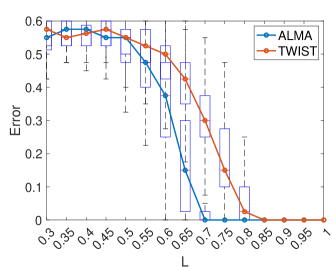
(a) Between-layer clustering

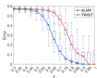
(b) Within-layer clustering

Figure 2: Simulation Scenario 1: $L=40,n=100,M=3,K=3,\alpha=0.9$. The between-layer clustering errors and within-layer clustering errors are plotted versus $p_{max}$. The solid lines exhibit the average misclassification errors.

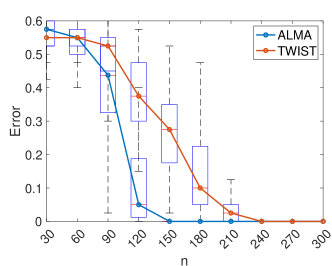
(a) Between-layer clustering

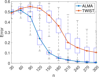
(b) Within-layer clustering

Figure 3: Simulation Scenario 2: $L=40,M=3,K=3,p_{max}=0.6,\alpha=0.9$. The between-layer clustering errors and within-layer clustering errors are plotted versus the number of vertices $n$. The solid lines exhibit the average misclassification errors.

We investigate the performances of ALMA (Algorithm 1) and compare it with the performances of the TWIST in four simulation scenarios. In our simulations, we set $M=3$, $K=3$ and $r=7$, since $r=\mathrm{rank}([\mbox{$\Theta$}_{1},\cdots,\mbox{$\Theta$}_{M}])\leq\sum_{m=1}^{M}K_{m}-(M-1)$, with inequality occurring in degenerate setting. Since our approach does not involve the concept of global membership, we only compare ALMA with TWIST in terms of “within–layer” and “between–layer clustering”. Furthermore, we choose the stopping criterion $\|\mathbf{W}^{(\mathrm{iter})}-\mathbf{W}^{(\mathrm{iter}-1)}\|\leq 10^{-4}$ for both of ALMA and TWIST to make a fair comparison between the algorithms. Below we describe the simulation schemes.

In Simulation 1, we investigate the effect of the network sparsity on the precision of the algorithms. For this purpose, we choose the number of vertices $n=100$, the number of layers $L=40$, the number of network clusters $M=3$, the number of communities in each cluster of layers $K=3$ and $\alpha=0.9$. The variable $p_{max}$, which controls the overall network sparsity, varies from $0.3$ to $1$. Fig. 2 shows that both between-layer and within-layer clustering errors decrease as $p_{max}$ is increasing.

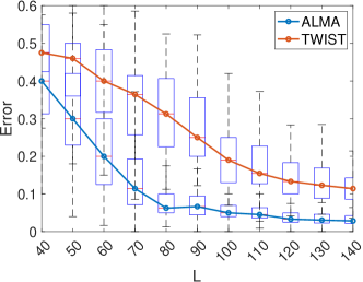
(a) Between-layer clustering

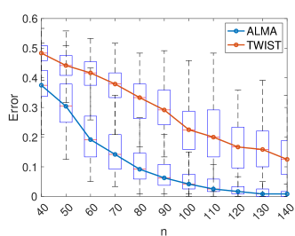
(b) Within-layer clustering

Figure 4: Simulation Scenario 3: $n=40,M=3,K=3,p_{max}=0.5,\alpha=0.8$. The between-layer clustering errors and within-layer clustering errors are plotted versus the number of layers $L$ when $L>n$. The solid lines exhibit the average misclassification errors.

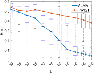
(a) Between-layer clustering

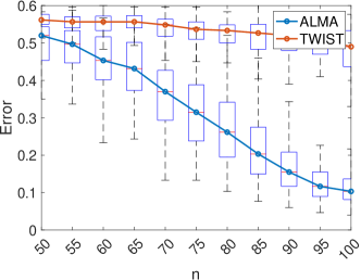
(b) Within-layer clustering

Figure 5: Simulation Scenario 4: $n=100,M=3,K=3,p_{max}=0.5,\alpha=0.9$. The between-layer clustering errors and within-layer clustering errors are plotted versus the number of layers $L$ when $L<n$. The solid lines exhibit the average misclassification errors.

In Simulation 2, the settings are the same as Simulation 1 except that $p_{max}=0.6$ is fixed, and the number of vertices varies from $30$ to $300$. As $n$ increases, the between-layer and within-layer clustering error rates decrease to zero, as predicted by Theorem 2.

In Simulations 3 and 4, we study the effect of the numbers of layers in the network, when $L>n$ and $L<n$, respectively. Specifically, in Simulation 3, we set $n=40,M=3,K=3,\alpha=0.8,p_{max}=0.6$ and vary the number of layers $L$ between $40$ and $140$. The settings in Simulation 4 are the same as Simulation 3, except $n=100$ is larger, and $L$ varies from $50$ to $100$.

For both algorithms, in each of the simulation scenarios, we report the between-layer and the within-layer clustering errors (27) and (28), respectively, averaged over 100 independent simulation runs. The results are summarized in Figures 2–5.

As it is evident from Figures 2–5, for all four scenarios, ALMA has smaller both the between-layer and the within-layer clustering errors. Note also that ALMA has better precision not only in the case of $L>n$, that violates the assumptions of TWIST, but also in the case of $L\leq n$.

6 Appendix

6.1 Manifold and tangent space

The concepts of tangent vector and tangent space to an abstract manifold can be found in, e.g., Boothby and Boothby (2003) and Absil et al. (2009). When ${\mathcal{M}}$ is a manifold embedded in the Euclidean space $\mathbb{R}^{p}$, then a smooth function $\gamma:\mathbb{R}\rightarrow{\mathcal{M}}$ is called a curve in ${\mathcal{M}}$, and $\gamma^{\prime}(0)$ is a tangent vector to the manifold ${\mathcal{M}}$ at the point $\gamma(0)$. The tangent space of ${\mathcal{M}}$ at $x$, denoted by $T_{x}{\mathcal{M}}$, is the set of all tangent vectors of ${\mathcal{M}}$ at $\mathbf{x}$, that is, $T_{x}{\mathcal{M}}=\{\gamma^{\prime}(0):\text{$\gamma:\mathbb{R}\rightarrow{\mathcal{M}}$ is a smooth function with $\gamma(0)=x$}\}$ (Absil and Oseledets, 2015). Intuitively, the tangent plane $T_{x}{\mathcal{M}}$ is the subspace that approximates the manifold ${\mathcal{M}}$ in a local neighborhood around $x$. For example, if ${\mathcal{M}}$ is the unit sphere $\{x=(x_{1},x_{2},x_{3}):x_{1}^{2}+x_{2}^{2}+x_{3}^{2}=1\}$, then the tangent space at point $(\hat{x}_{1},\hat{x}_{2},\hat{x}_{3})$ is given by $\{(x_{1},x_{2},x_{3}):\hat{x}_{1}x_{1}+\hat{x}_{2}x_{2}+\hat{x}_{3}x_{3}=0$}. A visualization of the tangent space is given in Figure 6.

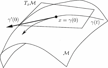
Figure 6: A visualization of the manifold ${\mathcal{M}}$, the curve $\gamma$ in ${\mathcal{M}}$, the tangent vector $\gamma^{\prime}(0)$, and the tangent space $T_{\mathbf{x}}({\mathcal{M}})$.

It remains to derive the tangent planes to the sets ${\mathcal{S}}_{1}$ and ${\mathcal{S}}_{2}$ at $\boldsymbol{Q}_{*}$ in (13). The expression for $L_{1}$ follows from the formula for the tangent planes for the manifold of low-rank matrices (Absil and Oseledets, 2015, equation (13)). Specifically, the explicit formula for the tangent plane to the manifold of rank $K$ matrices at $\mathbf{Q}$ is given by the equation $\Pi_{\mathbf{U}^{\perp}}\boldsymbol{Q}\Pi_{\mathbf{U}^{\perp}}=\mathbf{0}$, where $\mathbf{U}$ is an orthogonal matrix that has the same column space as $\mathbf{Q}$. Now, the first formula in (13) is due to the fact that ${\mathcal{S}}_{1}$ is the product of $M$ manifolds of low-rank matrices: ${\mathcal{S}}_{1}=\otimes_{m=1}^{M}{\mathcal{M}}_{m}$, where

$${\mathcal{M}}_{m}=\{\mathbf{X}\in\mathbb{R}^{n\times n}:\mathrm{rank}(\mathbf{X})\leq K_{m}\}.$$

In order to obtain the second equation in (13), note that the tangent plane to the set of orthogonal matrices ${\mathcal{M}}_{0}$ at $\mathbf{I}$ is the set of skew-symmetric matrices: $T_{\mathbf{I}}{\mathcal{M}}_{0}=\mathrm{Skew}_{M}$ (Edelman et al., 1998, Section 2.2.1). Now, the explicit formula for $L_{2}$ follows from the facts that ${\mathcal{S}}_{2}$ is obtained by multiplying $\boldsymbol{Q}_{*}$ with each element from ${\mathcal{M}}_{0}$, where ${\mathcal{M}}_{0}$ is the set of orthogonal matrices of size $M\times M$: ${\mathcal{S}}_{2}=\{\boldsymbol{Q}=\boldsymbol{Q}_{*}\times_{1}\mathbf{V}:\mathbf{V}\in{\mathcal{M}}_{0}\}$.

6.2 Proof of Theorem 1

The organization of this section follows from the sketch of the proof after Theorem 1 in four steps: the first step establishes a deterministic bound of $\mathbf{W}^{(\mathrm{iter})}-\mathbf{W}_{*}$, the second and the third steps establish a probabilistic bound, and the fourth step simplifies the probabilistic bound using Assumptions (A2)-(A4).

6.2.1 Step 1: Deterministic analysis of Algorithm 1

In this step, we aim to find a metric $\|\cdot\|_{d}$ on $\mathbb{R}^{L\times M}$ such that $\{\|\mathbf{W}^{(\mathrm{iter})}-\mathbf{W}_{*}\|_{d}\}_{\mathrm{iter}=1}^{\infty}$ should be monotonically decreasing approximately. While it is natural to consider the Frobenius norm, the previous analysis of the noiseless case in algorithm (12) does not support the monotonicity of $\{\|\mathbf{W}^{(\mathrm{iter})}-\mathbf{W}_{*}\|_{F}\}_{\mathrm{iter}=1}^{\infty}$. Instead, it establishes the “approximate” monotonicity of $\|\boldsymbol{Q}_{*}\times_{1}(\mathbf{V}^{(\mathrm{iter})}-\mathbf{I})\|_{F}$ of

$$\|\boldsymbol{Q}_{*}\times_{1}(\mathbf{V}^{(\mathrm{iter}+1)}-\mathbf{I})\|_{F}\lesssim\kappa_{H}\|\boldsymbol{Q}_{*}\times_{1}(\mathbf{V}^{(\mathrm{iter})}-\mathbf{I})\|_{F}.$$ (37)

Recall that in the noiseless case, $\mathbf{W}^{(\mathrm{iter})}=\mathbf{W}_{*}\mathbf{V}^{(\mathrm{iter})}$, we expect that $\|\cdot\|_{d}$ should be defined such that when $\mathbf{V}$ is orthogonal and close to $\mathbf{I}$,

$$\|\mathbf{W}_{*}(\mathbf{V}-\mathbf{I})\|_{d}\approx\|\boldsymbol{Q}_{*}\times_{1}(\mathbf{V}-\mathbf{I})\|_{F}.$$ (38)

Since the tangent plane of the set of orthogonal matrices at $\mathbf{I}$ is the set of skew-symmetric matrices (Gallier, 2001, Theorem 14.2.2), the tangent space of $\{\mathbf{W}_{*}\mathbf{V}:\mathbf{V}^{T}\mathbf{V}=\mathbf{I}\}$ at $\mathbf{V}=\mathbf{I}$ is $L_{0}=\{\mathbf{W}_{*}\mathbf{Y}:\mathbf{Y}\in\mathrm{Skew}_{M}\}\subseteq\mathbb{R}^{L\times M}$, (38) implies that for any $\mathbf{W}_{*}\mathbf{Y}\in L_{0}$, $\|\cdot\|_{d}$ should be defined such that $\|\mathbf{W}_{*}\mathbf{Y}\|_{d}=\lambda\|\boldsymbol{Q}_{*}\times_{1}\mathbf{Y}\|_{F}=\lambda\|\boldsymbol{P}_{*}\times_{1}\mathbf{W}_{*}\mathbf{Y}\|_{F}$ for some constant $\lambda>0$. Combining this metric on $L_{0}$ and the standard Euclidean/Frobenius metric on the orthogonal subspace $L_{0}^{\perp}$, we define the metric $\|\cdot\|_{d}:\mathbb{R}^{L\times M}\rightarrow\mathbb{R}$ by

$$\|\mathbf{W}\|_{d}=\sqrt{(\lambda\|\boldsymbol{P}_{*}\times_{1}P_{L_{0}}\mathbf{W}\|_{F})^{2}+\|P_{L_{0}^{\perp}}\mathbf{W}\|_{F}^{2}},$$ (39)

Here, $\lambda$ balances the weights from the two components, so that

$$\lambda=\left({\min_{\mathbf{Y}\in\mathrm{Skew}_{M},\,\|\mathbf{Y}\|_{F}=1}\|\boldsymbol{Q}_{*}\times_{1}\mathbf{Y}\|_{F}}\right)^{-1},$$

and the projection operators can be explicitly written as

$$P_{L_{0}}\mathbf{W} =\mathbf{W}_{*}(\mathbf{W}_{*}^{T}\mathbf{W}^{(\mathrm{iter})}-\mathbf{W}^{(\mathrm{iter})\,T}\mathbf{W}_{*})/2,$$

$$P_{L_{0}^{\perp}}\mathbf{W} =\mathbf{W}_{*}(\mathbf{W}_{*}^{T}\mathbf{W}^{(\mathrm{iter})}+\mathbf{W}^{(\mathrm{iter})\,T}\mathbf{W}_{*})/2+(\mathbf{I}-\mathbf{W}_{*}\mathbf{W}_{*}^{T})\mathbf{W}^{(\mathrm{iter})}.$$

By the definition of the metric $\|\cdot\|_{d}$ in (39), we have the following equivalence between $\|\cdot\|_{d}$ and $\|\cdot\|_{F}$:

$$\|\mathbf{W}\|_{d}\geq\sqrt{\|P_{L_{0}}\mathbf{W}\|_{F}^{2}+\|P_{L_{0}^{\perp}}\mathbf{W}\|_{F}^{2}}=\|\mathbf{W}\|_{F}$$

and for $C_{H}={{\displaystyle\max_{{\mathbf{Y}\in\mathrm{Skew}_{M},\,\|\mathbf{Y}\|_{F}=1}}\,\|\boldsymbol{Q}_{*}\times_{1}\mathbf{Y}\|_{F}}/\displaystyle\min_{{\mathbf{Y}\in\mathrm{Skew}_{M},\,\|\mathbf{Y}\|_{F}=1}}\,\|\boldsymbol{Q}_{*}\times_{1}\mathbf{Y}\|_{F}}$,

$$\|\mathbf{W}\|_{d}\leq\sqrt{C_{H}^{2}\|P_{L_{0}}\mathbf{W}\|_{F}^{2}+C_{H}^{2}\|P_{L_{0}^{\perp}}\mathbf{W}\|_{F}^{2}}=C_{H}\|\mathbf{W}\|_{F}.$$

Before stating our main result, we introduce two additional parameters:

$$\kappa_{1}=\frac{p_{\max}^{2}n^{2}{L}}{\|\boldsymbol{Q}_{*}\|_{F}^{2}},\quad\kappa_{2}=\frac{\sqrt{\dot{K}\,p_{\max}L}\ n}{\displaystyle\min_{m=1,....M}\ \,\sigma_{K_{m}}(\boldsymbol{Q}_{*}(m,:,:))}.$$

Both parameters are greater than $1$, and describe how “well-conditioned” $\boldsymbol{Q}_{*}$ is, and when $\boldsymbol{Q}_{*}$ is well-conditioned, then all parameters are close to $1$. In particular, $\kappa_{1}\geq 1$ because $\|\boldsymbol{Q}_{*}\|_{F}=\|\boldsymbol{P}_{*}\|_{F}$ and all elements of $\boldsymbol{P}_{*}$ are bounded by $p_{\max}$, and $\kappa_{2}\geq 1$ because

$$\dot{K}\min_{m=1,\cdots,M}\sigma_{K_{m}}^{2}(\boldsymbol{Q}_{*}(m,:,:))\leq\sum_{m=1}^{M}\sum_{k=1}^{K_{m}}\sigma_{k}^{2}(\boldsymbol{Q}_{*}(m,:,:))=\|\boldsymbol{Q}_{*}\|_{F}^{2}\leq p_{\max}^{2}n^{2}L.$$

When $\boldsymbol{Q}_{*}(m,:,:)$ is “degenerate” in the sense that $\sigma_{K_{m}}(\boldsymbol{Q}_{*}(m,:,:))\approx 0$, then $\kappa_{2}$ is large.

The main result in this step states that, if the noise $\boldsymbol{\Delta}$ is small and when Algorithm 1 is applied to the observed adjacency tensor $\boldsymbol{A}$ with a good initialization $\mathbf{W}^{(0)}$, the estimations are likely to improve over each iteration, and Algorithm 1 converges to $\mathbf{W}_{*}$ approximately. The statement is as follows, and its proof is rather complicated and deferred to Section 6.4.

Lemma 2 (Step 1: A deterministic result on Algorithm 1).

For

$$a_{1}= 6\kappa_{0}\frac{\sqrt{M}\left(\displaystyle\max_{m=1,....M}\ \|\Pi_{T,K_{m}}(\boldsymbol{\Delta})\times_{2,3}\Pi_{T,K_{m}}(\boldsymbol{\Delta})\|+2\displaystyle\max_{m=1,....M}\ \|\Pi_{T,K_{m}}(\boldsymbol{Q}_{*})\times_{2,3}\Pi_{T,K_{m}}(\boldsymbol{\Delta})\|\right)}{\sigma_{M}(\boldsymbol{Q}_{*}\times_{2,3}\boldsymbol{Q}_{*})}$$

$$+ \frac{192\kappa_{0}\dot{K}\|\boldsymbol{\Delta}\|^{2}(\|\boldsymbol{Q}_{*}\|+\|\boldsymbol{\Delta}\|)}{\sqrt{M}\left(\displaystyle\min_{m=1,....M}\ \sigma_{K_{m}}(\boldsymbol{Q}_{*}(m,:,:))\right)\ \sigma_{M}(\boldsymbol{Q}_{*}\times_{2,3}\boldsymbol{Q}_{*})},$$

$$a_{2}= \frac{192\kappa_{0}\dot{K}\|\boldsymbol{Q}_{*}\|^{2}(\|\boldsymbol{Q}_{*}\|+\|\boldsymbol{\Delta}\|)}{\sqrt{M}\displaystyle\min_{m=1,....M}\ \sigma_{K_{m}}(\boldsymbol{Q}_{*}(m,:,:))\ \sigma_{M}(\boldsymbol{Q}_{*}\times_{2,3}\boldsymbol{Q}_{*})}+6\kappa_{0},$$

if $\|\boldsymbol{\Delta}\|\leq\frac{1}{4}\displaystyle\min_{m=1,....M}\ \sigma_{K_{m}}(\boldsymbol{Q}_{*}(m,:,:))$,

$$\frac{2C_{H}a_{1}}{1-\kappa_{H}}\leq\min\Big{(}\frac{1-\kappa_{H}}{2C_{H}(a_{2}+80\kappa_{0}^{2}+32\kappa_{0}^{3})},\frac{\min_{m=1,\cdots,M}\sigma_{K_{m}}(\boldsymbol{Q}_{*}(m,:,:))}{4\|\boldsymbol{Q}_{*}\|}\Big{)}$$ (40)

and the initialization satisfies

$$\|\mathbf{W}^{(1)}-\mathbf{W}_{*}\|_{d}\leq\min\left(\frac{1-\kappa_{H}}{2C_{H}(a_{2}+80\kappa_{0}^{2}+32\kappa_{0}^{3})},\frac{\min_{m=1,\cdots,M}\sigma_{K_{m}}(\boldsymbol{Q}_{*}(m,:,:))}{4\|\boldsymbol{Q}_{*}\|}\right),$$ (41)

then for all $\mathrm{iter}\geq 1$,

$$\|\mathbf{W}^{(\mathrm{iter}+1)}-\mathbf{W}_{*}\|_{d}\leq\frac{1+\kappa_{H}}{2}\|\mathbf{W}^{(\mathrm{iter})}-\mathbf{W}_{*}\|_{d}+C_{H}a_{1},$$ (42)

which implies

$$\lim_{\mathrm{iter}\rightarrow\infty}\|\mathbf{W}^{(\mathrm{iter})}-\mathbf{W}_{*}\|_{d}\leq\frac{2C_{H}a_{1}}{1-\kappa_{H}}.$$

6.2.2 Step 2: Probabilistic estimation

Since $\boldsymbol{Q}_{*}$ is deterministic in our model, we only need to estimate the terms that depend on $\boldsymbol{\Delta}$ in Lemma 2. The estimations are summarized as follows, and the proof is deferred to the Appendix.

Lemma 3 (Step 2: Probabilistic estimation).

(a) [Restatement of (Zhou and Zhu, 2019, Theorem 1.2)] If $p_{\max}\geq\frac{c\log(\max(n,L))}{\max(n,L)}$ for some constant $c>0$, then for any $r>0$, there exists a constant $C>0$ depending only on $r,c$ such that with probability at least $1-n^{-r}$, $\|\boldsymbol{\Delta}\|=\sup_{\mathbf{u}\in\mathbb{R}^{L},\mathbf{v}\in\mathbb{R}^{n}}\frac{\boldsymbol{\Delta}\times_{1}\mathbf{u}\times_{2}\mathbf{v}\times_{3}\mathbf{v}}{\|\mathbf{u}\|\|\mathbf{v}\|^{2}}$ satisfies $\|\boldsymbol{\Delta}\|\leq C\sqrt{p_{\max}\max(n,L)}\log(\max(n,L))$.
(b) For any $t>0$,

$$\Pr\left(\Big{\|}\Pi_{T,K_{m}}(\boldsymbol{Q}_{*})\times_{2,3}\Pi_{T,K_{m}}(\boldsymbol{\Delta})\Big{\|}_{F}>3tnL\sqrt{p_{\max}^{3}}\right)\leq 2\dot{K}L\exp\left(\frac{-\frac{1}{2}t^{2}}{1+\frac{t}{3\sqrt{p_{\max}ng_{\min}}}}\right).$$ (43)

(c) For any $t>0$,

$$\Pr\left(\max_{1\leq m\leq M}\|\Pi_{T,K_{m}}(\boldsymbol{\Delta})\times_{2,3}\Pi_{T,K_{m}}(\boldsymbol{\Delta})\|\geq 9K^{2}t^{2}{p_{\max}\max(n,L)}\right)$$ (44)

$$\leq 2K(L+n)\exp\left(-\frac{t^{2}/2}{1+\frac{t}{\sqrt{p_{\max}\max(n,L)g_{\min}}}}\right),$$

where $g_{\min}$ is the size of the smallest community.

6.2.3 Step 3: A probabilistic result on Algorithm 1 without Assumptions (A2)-(A4)

From the definition of $\kappa_{0}=\frac{\sigma_{1}(\boldsymbol{Q}_{*}\times_{2,3}\boldsymbol{Q}_{*})}{\sigma_{M}(\boldsymbol{Q}_{*}\times_{2,3}\boldsymbol{Q}_{*})}$ and the fact $\boldsymbol{Q}_{*}\times_{2,3}\boldsymbol{Q}_{*}={\mathcal{M}}_{1}(\boldsymbol{Q}_{*}){\mathcal{M}}_{1}(\boldsymbol{Q}_{*})^{T}$, we have

$$\kappa_{0}=\left(\frac{\sigma_{1}(\boldsymbol{Q}_{*}\times_{2,3}\boldsymbol{Q}_{*})}{\sigma_{M}(\boldsymbol{Q}_{*}\times_{2,3}\boldsymbol{Q}_{*})}\right)=\left(\frac{\sigma_{1}({\mathcal{M}}_{1}(\boldsymbol{Q}_{*}))}{\sigma_{M}({\mathcal{M}}_{1}(\boldsymbol{Q}_{*}))}\right)^{2},$$

$\|\boldsymbol{Q}_{*}\times_{1}\!\mathbf{Y}\|_{F}\!=\!\!\|{\mathcal{M}}_{1}(\boldsymbol{Q}_{*})\mathbf{Y}\|_{F}\!\leq\!\sigma_{1}\!({\mathcal{M}}_{1}(\boldsymbol{Q}_{*}))\|\!\mathbf{Y}\!\|_{F},$ and $\|\boldsymbol{Q}_{*}\times_{1}\!\mathbf{Y}\!\|_{F}\!=\!\!\|{\mathcal{M}}_{1}(\boldsymbol{Q}_{*}\!)\mathbf{Y}\|_{F}\!\!\geq\!\sigma_{M}({\mathcal{M}}_{1}(\boldsymbol{Q}_{*}\!))\|\mathbf{Y}\|_{F}$. As a result, $C_{H}\leq\sqrt{\kappa_{0}}$.

Combining $C_{H}\leq\sqrt{\kappa_{0}}$ with $\|\boldsymbol{Q}_{*}\|\leq\|\boldsymbol{Q}_{*}\|_{F}\leq p_{\max}n\sqrt{L}$, one obtains

$$\sigma_{M}(\boldsymbol{Q}_{*}\times_{2,3}\boldsymbol{Q}_{*})\geq\frac{1}{\kappa_{0}}\sigma_{1}(\boldsymbol{Q}_{*}\times_{2,3}\boldsymbol{Q}_{*})=\frac{1}{\kappa_{0}}\|{\mathcal{M}}_{1}(\boldsymbol{Q}_{*})\|^{2}\geq\frac{1}{M\kappa_{0}}\|{\mathcal{M}}_{1}(\boldsymbol{Q}_{*})\|_{F}^{2}=\frac{1}{M\kappa_{0}}\|\boldsymbol{Q}_{*}\|_{F}^{2}\geq\frac{p_{\max}^{2}n^{2}L}{M\kappa_{0}\kappa_{1}},$$

Then, Lemma 2 and Lemma 3 imply the following statement.

Theorem 3 (Step 3: A generic result on Algorithm 1 without Assumptions (A2)-(A4)).

If

$$p_{\max}\geq\frac{c\log(\max(n,L))}{\max(n,L)} c>0$$ for some constant , (45)

then for any $r>0$, there exists $C>0$ that depending only on $r,c$ such that for

$$a_{1}= C\kappa_{0}^{2}\kappa_{1}\sqrt{M^{3}}\Big{(}\frac{t}{n\sqrt{p_{\max}}}+\frac{\dot{K}^{2}t^{2}}{p_{\max}n\min(n,L)}\Big{)}+{C\kappa_{0}^{2}\kappa_{1}\kappa_{2}\sqrt{M\dot{K}}}\frac{\log^{2}(\max(n,L))}{{p_{\max}}n\min(n,L)}$$

$$a_{2}= {C\kappa_{0}^{2}\kappa_{1}\kappa_{2}\sqrt{M\dot{K}}}\Big{(}1+\frac{\log(\max(n,L))}{\sqrt{p_{\max}n\min(n,L)}}\Big{)},$$

if

$$C\kappa_{2}\sqrt{{\dot{K}}}\leq\sqrt{{p_{\max}n\min(n,L)}},\,\,\,\sqrt{4a_{1}\kappa_{0}(a_{2}+112\kappa_{0}^{3})}\leq 1-\kappa_{H},\,\,\,2\kappa_{0}\kappa_{2}a_{1}\sqrt{\dot{K}}\leq(1-\kappa_{H})$$ (46)

and the initialization satisfies

$$\|\mathbf{W}^{(1)}-\mathbf{W}_{*}\|_{F}\leq\min\Big{(}\frac{1-\kappa_{H}}{2\kappa_{0}(a_{2}+112\kappa_{0}^{3})},\frac{1}{4\kappa_{2}\sqrt{\kappa_{0}\dot{K}}}\Big{)}$$ (47)

then with probability at least

$$1-n^{-r}-2\dot{K}L\exp\left(\frac{-\frac{1}{2}t^{2}}{1+\frac{t}{3\sqrt{p_{\max}ng_{\min}}}}\right)-2K(L+n)\exp\left(-\frac{t^{2}/2}{1+\frac{t}{\sqrt{p_{\max}\max(n,L)g_{\min}}}}\right),$$

$$\|\mathbf{W}^{(\mathrm{iter}+1)}-\mathbf{W}_{*}\|_{d}\leq\frac{1+\kappa_{H}}{2}\|\mathbf{W}^{(\mathrm{iter})}-\mathbf{W}_{*}\|_{d}+a_{1}\sqrt{\kappa_{0}},$$ (48)

holds for all $\mathrm{iter}\geq 1$, which implies

$$\lim_{\mathrm{iter}\rightarrow\infty}\|\mathbf{W}^{(\mathrm{iter})}-\mathbf{W}_{*}\|_{F}\leq\lim_{\mathrm{iter}\rightarrow\infty}\|\mathbf{W}^{(\mathrm{iter})}-\mathbf{W}_{*}\|_{d}\leq\frac{2a_{1}\sqrt{\kappa_{0}}}{1-\kappa_{H}}.$$

6.2.4 Step 4: Simplification under Assumptions (A2)-(A4)

We will need to estimate the parameters $\kappa_{1},\kappa_{2}$ under Assumptions (A2)-(A4). Since $\boldsymbol{Q}_{*}(m,:,:)=\sqrt{L_{m}}\mbox{$\Theta$}_{m}\mathbf{B}_{m}\mbox{$\Theta$}_{m}^{T}$ and $\mbox{$\Theta$}_{m}^{T}\mbox{$\Theta$}_{m}=\mbox{diag}(|G_{m,1}|,|G_{m,2}|,\cdots,|G_{m,K_{m}}|)$, we have $\sigma_{K_{m}}(\boldsymbol{Q}_{*}(m,:,:))\geq\sqrt{L_{m}}\sigma_{K_{m}}(\mathbf{B}_{m})\sigma_{K_{m}}(\mbox{$\Theta$}_{m})^{2}\geq{c_{1}\sqrt{c_{3}}}p_{\max}\frac{n\sqrt{L}}{K_{m}\sqrt{M}}\min_{m=1,\cdots,M}\sigma_{K_{m}}(\mathbf{B}_{m}^{0})$, which suggests

$$\kappa_{2}\leq\frac{K_{\max}\sqrt{M}}{c_{1}\sqrt{c_{3}}b_{1}}.$$

Similarly, we have the estimation

$$\kappa_{1}\leq\frac{1}{c_{1}c_{3}^{2}b_{2}}.$$

Let $p^{*}=p_{\max}n\min(n,L)$ and $t=\log(n+L)$, then we have the estimation that

$$a_{1}= \frac{C\kappa_{0}^{2}\sqrt{M^{3}}}{c_{1}c_{3}^{2}b_{2}}\Big{(}\frac{t}{n\sqrt{p_{\max}}}+\frac{\dot{K}^{2}t^{2}}{p_{\max}n\min(n,L)}\Big{)}+{C\kappa_{0}^{2}\frac{\sqrt{\dot{K}}K_{\max}M}{c_{1}^{1.5}c_{3}^{3}b_{1}b_{2}}}\frac{\log^{2}(\max(n,L))}{p_{\max}n\min(n,L)}$$

$$\leq C\kappa_{0}^{2}\log^{2}(n+L)\left(\frac{1}{\sqrt{p_{\max}n^{2}}}\frac{\sqrt{M^{3}}}{c_{1}c_{3}^{2}b_{2}}+\frac{1}{p^{*}}\Big{(}\frac{\dot{K}^{2}\sqrt{M^{3}}}{c_{1}c_{3}^{2}b_{2}}+\frac{\sqrt{\dot{K}}K_{\max}M}{c_{1}^{1.5}c_{3}^{3}b_{1}b_{2}}\Big{)}\right)$$

$$\leq C\kappa_{0}^{2}\log^{2}(n+L)\sqrt{M^{3}}\left(\sqrt{\frac{1}{p_{\max}n^{2}}}+\frac{\dot{K}^{2}}{p^{*}}\right)$$

$$a_{2}= C\kappa_{0}^{2}\frac{\sqrt{\dot{K}}K_{\max}M}{c_{1}^{1.5}c_{3}^{3}b_{1}b_{2}}\Big{(}1+\frac{\log(\max(n,L))}{\sqrt{p_{\max}n\min(n,L)}}\Big{)}\leq C\kappa_{0}^{3}\log(n+L)\frac{1}{\sqrt{p^{*}}}\frac{\sqrt{\dot{K}}K_{\max}M}{c_{1}^{1.5}c_{3}^{3}b_{1}b_{2}}$$

$$\leq C\kappa_{0}^{2}\log(n+L)\sqrt{\frac{\dot{K}^{3}}{p^{*}}},$$

By calculation, a sufficient condition for the requirement in (46) becomes (18).

With (18), we have $\frac{p^{*}(1-\kappa_{H})}{\kappa_{0}^{2}\log(n+L)\dot{K}^{3}}\geq\frac{\sqrt{M}}{\dot{K}^{2}}$. Combining it with $a_{2}\geq{C\kappa_{0}^{2}\kappa_{1}\kappa_{2}\sqrt{M\dot{K}}}\Big{(}1+\frac{\log(\max(n,L))}{\sqrt{p^{*}}}\Big{)}$, the assumption on the initialization (47) can be guaranteed by (19). In addition, (45) and (46) follow from (18). Then (20) is proved by applying Theorem 3, and (21) follows from (20). The proof of (22) is presented in (26) at the end of Section 4.3.

6.3 Proof of Theorem 2

Proof of Theorem 2.

(a) For completeness, we will first write down the statement from (Lei, 2020, Lemma C.1):

Let $\mathbf{U}$ be an $n\times d$ matrix with $K$ distinct rows with minimum pairwise Euclidean norm separation $\gamma$. Let $\hat{\mathbf{U}}$ be another $n\times d$ matrix and $(\hat{\mbox{$\Theta$}},\hat{\mathbf{X}})$ be an $(1+\epsilon)$-approximate solution to K-means problem with input $\hat{\mathbf{U}}$, then the number of errors in $\hat{\mbox{$\Theta$}}$ as an estimate of the row clusters of $\mathbf{U}$ is no larger than $C_{\epsilon}\|\mathbf{U}-\hat{\mathbf{U}}\|_{F}^{2}\gamma^{-2}$ for some constant $C_{\epsilon}$ depending only on $\epsilon$.

Note that $\mathbf{W}_{*}$ is an $L\times M$ matrix with $M$ distinct rows with minimum pairwise Euclidean norm separation larger than $2/\max_{m=1,\cdots,M}\sqrt{L_{m}}$, the misclassification rate is not larger than

$$\frac{\max_{m=1,\cdots,M}L_{m}}{4L}C_{\epsilon}\|\mathbf{W}_{*}-\hat{\mathbf{W}}\|_{F}^{2}.$$

Combining it with the estimation of $\|\mathbf{W}_{*}-\hat{\mathbf{W}}\|_{F}^{2}$ and assumption (A3) on $\frac{\max_{m=1,\cdots,M}L_{m}}{L}$, part (a) is proved.

(b) Denote the orthogonal matrix of size $n\times K_{m}$ whose columns are the top $K_{m}$ eigenvectors of $\widehat{\boldsymbol{Q}}(m,:,:)$ by $\hat{\mathbf{U}}_{m}$ and the orthogonal matrix of size $n\times K_{m}$ whose columns are the top $K_{m}$ eigenvectors of ${\boldsymbol{Q}}_{*}(m,:,:)$ by $\mathbf{U}_{m}$, then the Davis-Kahan theorem implies that

$$\|\hat{\mathbf{U}}_{m}-{\mathbf{U}}_{m}\|_{F}\leq\frac{\|\widehat{\boldsymbol{Q}}(m,:,:)-\boldsymbol{Q}_{*}(m,:,:)\|_{F}}{\sigma_{K_{m}}(\boldsymbol{Q}_{*}(m,:,:))}.$$

In addition, ${\mathbf{U}}_{m}$ has $K_{m}$ distinct rows with minimum pairwise Euclidean norm separation at least $2/\sqrt{g_{m,\max}}$, where $\displaystyle{g_{m,\max}=\max_{1\leq k\leq K_{m}}\,|G_{m,k}|}$. As a result, (22) implies that the misclassification rate is bounded by

$$\frac{g_{m,\max}}{4n}C_{\epsilon}\frac{\|\widehat{\boldsymbol{Q}}(m,:,:)-\boldsymbol{Q}_{*}(m,:,:)\|_{F}^{2}}{\sigma_{K_{m}}(\boldsymbol{Q}_{*}(m,:,:))^{2}}$$

$$\leq \frac{1}{4K_{m}}C_{\epsilon}\frac{\|\widehat{\boldsymbol{Q}}(m,:,:)-\boldsymbol{Q}_{*}(m,:,:)\|_{F}^{2}}{\sigma_{K_{m}}(\boldsymbol{Q}_{*}(m,:,:))^{2}}\leq C_{\epsilon}\frac{\|\widehat{\boldsymbol{Q}}(m,:,:)-\boldsymbol{Q}_{*}(m,:,:)\|^{2}}{\sigma_{K_{m}}(\boldsymbol{Q}_{*}(m,:,:))^{2}}$$

$$\leq C_{\epsilon}\frac{(2\|\boldsymbol{Q}_{*}\|\|\hat{\mathbf{W}}-\mathbf{W}_{*}\|_{F}+2\|\boldsymbol{\Delta}\|)^{2}}{\sigma_{K_{m}}(\boldsymbol{Q}_{*}(m,:,:))^{2}}\leq C_{\epsilon}\frac{(2p_{\max}n\sqrt{L}\|\hat{\mathbf{W}}-\mathbf{W}_{*}\|_{F}+2\|\boldsymbol{\Delta}\|)^{2}}{\sigma_{K_{m}}(\boldsymbol{Q}_{*}(m,:,:))^{2}}$$

$$\leq C_{\epsilon}(\frac{\kappa_{2}^{2}}{\dot{K}})\Bigg{(}\|\hat{\mathbf{W}}-\mathbf{W}_{*}\|_{F}^{2}+\Big{(}\frac{\sqrt{p_{\max}\max(n,L)}\log(\max(n,L))}{p_{\max}n\sqrt{L}}\Big{)}^{2}\Bigg{)}$$

$$\leq C_{\epsilon}(\frac{K_{\max}^{2}M}{\dot{K}})\Bigg{(}\|\hat{\mathbf{W}}-\mathbf{W}_{*}\|_{F}^{2}+\Big{(}\frac{\sqrt{p_{\max}\max(n,L)}\log(\max(n,L))}{p_{\max}n\sqrt{L}}\Big{)}^{2}\Bigg{)}$$

$$\leq C_{\epsilon}(\frac{K_{\max}^{2}M}{\dot{K}})\Bigg{(}\Big{(}\log^{2}(n+L)\sqrt{M^{3}}\frac{\sqrt{\kappa_{0}}}{1-\kappa_{H}}\Big{(}\sqrt{\frac{1}{p_{\max}n^{2}}}+\frac{\dot{K}^{2}}{p_{\max}n\min(n,L)}\Big{)}\Big{)}^{2}$$

$$+\Big{(}\frac{\sqrt{p_{\max}\max(n,L)}\log(\max(n,L))}{p_{\max}n\sqrt{L}}\Big{)}^{2}\Bigg{)}$$

$$\leq C_{\epsilon}K_{\max}\Bigg{(}\log^{4}(n+L){M^{3}}\frac{{\kappa_{0}}}{(1-\kappa_{H})^{2}}\Big{(}{\frac{1}{p_{\max}n^{2}}}+\frac{\dot{K}^{4}}{p_{\max}^{2}n^{2}\min(n,L)^{2}}\Big{)}+\frac{(n+L)\log(n+L)^{2}}{n^{2}{p_{\max}L}}\Bigg{)}$$

∎

6.4 Proof of Lemma 2

Proof of Lemma 2.

The main idea of the proof of Lemma 2 is as follows. Assumption (A1) implies that, when the observation is noise-free in the sense that $\boldsymbol{A}=\boldsymbol{P}_{*}$, Algorithm 1 converges linearly. As a result, we only need to show that the output of the algorithm does not change much if we replace $\boldsymbol{A}$ with $\boldsymbol{P}_{*}$ and Algorithm 1 with its linear approximation $P_{L_{2}}P_{L_{1}}$.

Given $\mathbf{W}^{(\mathrm{iter})}$, we construct a skew-symmetric matrix $\mathbf{Y}^{(\mathrm{iter})}\in\mathbb{R}^{M\times M}$ by

$$\mathbf{Y}^{(\mathrm{iter})}=\frac{1}{2}(\mathbf{W}_{*}^{T}\mathbf{W}^{(\mathrm{iter})}-\mathbf{W}^{(\mathrm{iter})\,T}\mathbf{W}_{*}),$$ (49)

and then the update formula for the “clean” version of the algorithm is the solution to the equation

$$\boldsymbol{Q}_{*}\times_{1}\hat{\mathbf{Y}}^{(\mathrm{iter}+1)}=P_{L_{2}}P_{L_{1}}(\boldsymbol{Q}_{*}\times_{1}\mathbf{Y}^{(\mathrm{iter})}).$$ (50)

Intuitively, $\hat{\mathbf{Y}}^{(\mathrm{iter}+1)}$ is the algorithmic update when $\boldsymbol{A}_{*}$ is replaced by $\boldsymbol{P}_{*}$, and Algorithm 1 is replaced by its linear approximation $P_{L_{2}}P_{L_{1}}$. By the definition of $\kappa_{H}$ in (14), we have

$$\|\mathbf{W}_{*}\hat{\mathbf{Y}}^{(\mathrm{iter}+1)}\|_{d}\leq\kappa_{H}\|\mathbf{W}_{*}{\mathbf{Y}}^{(\mathrm{iter})}\|_{d}.$$ (51)

We will bound $\|\mathbf{W}^{(\mathrm{iter}+1)}-\mathbf{W}_{*}\|_{d}$ as a function of $\|\mathbf{W}^{(\mathrm{iter})}-\mathbf{W}_{*}\|_{d}$ by (51) and the following perturbation bounds in Lemma 4, with its proof deferred to Section 6.4.1.

Lemma 4.

For any $\mathbf{W}^{\mathrm{iter}}$, let $\mathbf{Y}^{\mathrm{iter}}$ and $\hat{\mathbf{Y}}^{\mathrm{iter}+1}$ be defined as in (49) and (50), then

1. $$\|\mathbf{W}_{*}\mathbf{Y}^{(\mathrm{iter})}\|_{d}\leq\|\mathbf{W}^{(\mathrm{iter})}-\mathbf{W}_{*}\|_{d}.$$ (52)

2. For

   $$\tilde{\mathbf{W}}^{(\mathrm{iter}+1)}=\Pi_{o}(\boldsymbol{P}_{*}\times_{2,3}(\boldsymbol{Q}_{*}+\Pi_{T,\mathbf{K}}(\boldsymbol{Q}_{*}\times_{1}\mathbf{Y}^{(\mathrm{iter})}))),$$ (53)

   we have

   $$\|\tilde{\mathbf{W}}^{(\mathrm{iter}+1)}-\mathbf{W}_{*}(\hat{\mathbf{Y}}^{(\mathrm{iter}+1)}+\mathbf{I})\|_{F}\leq\frac{32\kappa_{0}^{2}\|\mathbf{Y}^{\mathrm{iter}}\|_{F}^{2}}{2-8\kappa_{0}^{2}\|\mathbf{Y}^{\mathrm{iter}}\|_{F}-4\kappa_{0}\|\mathbf{Y}^{\mathrm{iter}}\|_{F}(2+4\kappa_{0}\|\mathbf{Y}^{\mathrm{iter}}\|_{F})}$$

   $$+\Big{(}1+\frac{2\kappa_{0}+8\kappa_{0}\|\mathbf{Y}^{\mathrm{iter}}\|_{F}}{2-8\kappa_{0}\|\mathbf{Y}^{\mathrm{iter}}\|_{F}-\kappa_{0}(1+4\kappa_{0}\|\mathbf{Y}^{\mathrm{iter}}\|_{F})4\kappa_{0}\|\mathbf{Y}^{\mathrm{iter}}\|_{F}}\Big{)}(4\kappa_{0}\|\mathbf{Y}^{\mathrm{iter}}\|_{F})^{2}.$$ (54)

3. If

   $$\|\mathbf{W}_{*}-\mathbf{W}^{(\mathrm{iter})}\|_{F}\leq\frac{\min_{m=1,\cdots,M}\sigma_{K_{m}}(\boldsymbol{Q}_{*}(m,:,:))}{\|\boldsymbol{Q}_{*}\|},$$ (55)

   then,

   $$\|{\mathbf{W}}^{(\mathrm{iter}+1)}-\tilde{\mathbf{W}}^{(\mathrm{iter}+1)}\|_{F}\leq\frac{\beta_{1}}{\sigma_{M}(\boldsymbol{Q}_{*}\times_{2,3}\boldsymbol{Q}_{*})-2\|\boldsymbol{Q}_{*}\times_{2,3}\boldsymbol{Q}_{*}\|\|\mathbf{Y}^{(\mathrm{iter})}\|_{F}-\beta},$$ (56)

   where, for $a_{1}$ and $a_{2}$ are defined in Lemma 2,

   $$\beta_{1}=\frac{\sigma_{M}(\boldsymbol{Q}_{*}\times_{2,3}\boldsymbol{Q}_{*})}{6}(a_{1}+a_{2}\|\mathbf{W}_{*}-\mathbf{W}^{(\mathrm{iter})}\|_{F}^{2})$$

With the perturbation bounds (54) and (56) in Lemma 4, we have

$$\|\mathbf{W}^{(\mathrm{iter}+1)}-\mathbf{W}_{*}(\hat{\mathbf{Y}}^{(\mathrm{iter}+1)}+\mathbf{I})\|_{F}$$

$$\leq \|{\mathbf{W}}^{(\mathrm{iter}+1)}-\tilde{\mathbf{W}}^{(\mathrm{iter}+1)}\|_{F}+\|\tilde{\mathbf{W}}^{(\mathrm{iter}+1)}-\mathbf{W}_{*}(\hat{\mathbf{Y}}^{(\mathrm{iter}+1)}+\mathbf{I})\|_{F}$$

$$\leq \frac{\beta_{1}}{\sigma_{M}(\boldsymbol{Q}_{*}\times_{2,3}\boldsymbol{Q}_{*})-2\|\boldsymbol{Q}_{*}\times_{2,3}\boldsymbol{Q}_{*}\|\|\mathbf{Y}^{(\mathrm{iter})}\|_{F}-\beta_{1}}$$

$$+\frac{32\kappa_{0}^{2}\|\mathbf{Y}^{\mathrm{iter}}\|_{F}^{2}}{2-8\kappa_{0}^{2}\|\mathbf{Y}^{\mathrm{iter}}\|_{F}-4\kappa_{0}\|\mathbf{Y}^{\mathrm{iter}}\|_{F}(2+4\kappa_{0}\|\mathbf{Y}^{\mathrm{iter}}\|_{F})}$$

$$+ \Big{(}1+\frac{2\kappa_{0}+8\kappa_{0}\|\mathbf{Y}^{\mathrm{iter}}\|_{F}}{2-8\kappa_{0}\|\mathbf{Y}^{\mathrm{iter}}\|_{F}-\kappa_{0}(1+4\kappa_{0}\|\mathbf{Y}^{\mathrm{iter}}\|_{F})4\kappa_{0}\|\mathbf{Y}^{\mathrm{iter}}\|_{F}}\Big{)}(4\kappa_{0}\|\mathbf{Y}^{\mathrm{iter}}\|_{F})^{2}.$$

When

$$a_{1}\leq 1,\|\mathbf{W}^{(iter)}-\mathbf{W}_{*}\|_{F}\leq\min(\frac{1}{32\kappa_{0}^{3}},\frac{1}{\sqrt{a_{2}}}),$$ (57)

we have (using $\|\mathbf{Y}^{(iter)}\|_{F}\leq\|\mathbf{W}^{(iter)}-\mathbf{W}_{*}\|_{F}$) $4\kappa_{0}\|\mathbf{Y}^{\mathrm{iter}}\|_{F}\leq 1$, $8\kappa_{0}^{2}\|\mathbf{Y}^{\mathrm{iter}}\|_{F}+4\kappa_{0}\|\mathbf{Y}^{\mathrm{iter}}\|_{F}(2+4\kappa_{0}\|\mathbf{Y}^{\mathrm{iter}}\|_{F})<1$,  $8\kappa_{0}\|\mathbf{Y}^{\mathrm{iter}}\|_{F}+\kappa_{0}(1+4\kappa_{0}\|\mathbf{Y}^{\mathrm{iter}}\|_{F})4\kappa_{0}\|\mathbf{Y}^{\mathrm{iter}}\|_{F}<1$, which imply $\|\boldsymbol{Q}_{*}\times_{2,3}\boldsymbol{Q}_{*}\|\|\mathbf{Y}^{(\mathrm{iter})}\|_{F}\leq\sigma_{M}(\boldsymbol{Q}_{*}\times_{2,3}\boldsymbol{Q}_{*})/2$ and $\|\mathbf{W}_{*}-\mathbf{W}^{(\mathrm{iter})}\|_{F}^{2}\leq 1$, and

$$\|\mathbf{W}^{(\mathrm{iter}+1)}-\mathbf{W}_{*}(\hat{\mathbf{Y}}^{(\mathrm{iter}+1)}+\mathbf{I})\|_{F}$$ (58)

$$\leq \frac{\beta_{1}}{\sigma_{M}(\boldsymbol{Q}_{*}\times_{2,3}\boldsymbol{Q}_{*})(1-1/2-1/3)}+32\kappa_{0}^{2}\|\mathbf{Y}^{\mathrm{iter}}\|_{F}^{2}+(1+2\kappa_{0}+8\kappa_{0}\|\mathbf{Y}^{\mathrm{iter}}\|_{F})(4\kappa_{0}\|\mathbf{Y}^{\mathrm{iter}}\|_{F})^{2}$$

$$= \frac{6\beta_{1}}{\sigma_{M}(\boldsymbol{Q}_{*}\times_{2,3}\boldsymbol{Q}_{*})}+(3+2\kappa_{0}+8\kappa_{0}\|\mathbf{Y}^{\mathrm{iter}}\|_{F})(4\kappa_{0}\|\mathbf{Y}^{\mathrm{iter}}\|_{F})^{2}$$

$$\leq \frac{6\beta_{1}}{\sigma_{M}(\boldsymbol{Q}_{*}\times_{2,3}\boldsymbol{Q}_{*})}+(5+2\kappa_{0})(4\kappa_{0}\|\mathbf{Y}^{\mathrm{iter}}\|_{F})^{2}$$

$$= \kappa_{0}(a_{1}+a_{2}\|\mathbf{W}_{*}^{T}\mathbf{W}^{(\mathrm{iter})}-\mathbf{I}\|^{2})+(5+2\kappa_{0})(4\kappa_{0}\|\mathbf{Y}^{\mathrm{iter}}\|_{F})^{2}.$$

Combining (51), (52), and (58), we have

$$\|\mathbf{W}^{(\mathrm{iter}+1)}-\mathbf{W}_{*}\|_{d}\leq\|\mathbf{W}_{*}\hat{\mathbf{Y}}^{(\mathrm{iter}+1)}\|_{d}+\|\mathbf{W}^{(\mathrm{iter}+1)}-\mathbf{W}_{*}(\hat{\mathbf{Y}}^{(\mathrm{iter}+1)}+\mathbf{I})\|_{d}$$

$$\leq\kappa_{H}\|\mathbf{W}_{*}{\mathbf{Y}}^{(\mathrm{iter})}\|_{d}+\|\mathbf{W}^{(\mathrm{iter}+1)}-\mathbf{W}_{*}(\hat{\mathbf{Y}}^{(\mathrm{iter}+1)}+\mathbf{I})\|_{d}$$

$$\leq\kappa_{H}\|\mathbf{W}_{*}-{\mathbf{W}}^{(\mathrm{iter})}\|_{d}+\|\mathbf{W}^{(\mathrm{iter}+1)}-\mathbf{W}_{*}(\hat{\mathbf{Y}}^{(\mathrm{iter}+1)}+\mathbf{I})\|_{d}$$

$$\leq\!\kappa_{H}\|\mathbf{W}^{(\mathrm{iter})}\!\!-\!\mathbf{W}_{*}\|_{d}+\!C_{H}\Big{(}a_{1}\!+\!a_{2}\|\mathbf{W}_{*}-\mathbf{W}^{(\mathrm{iter})}\!-\!\mathbf{I}\|_{F}^{2}\!+\!(5\!+\!2\kappa_{0})(4\kappa_{0}\|\mathbf{Y}^{\mathrm{iter}}\|_{F})^{2}\!\Big{)}$$

$$\leq\kappa_{H}\|\mathbf{W}^{(\mathrm{iter})}-\mathbf{W}_{*}\|_{d}+C_{H}\Big{(}a_{1}+a_{2}\|\mathbf{W}_{*}-\mathbf{W}^{(\mathrm{iter})}\|_{F}^{2}+16(5+2\kappa_{0})\kappa_{0}^{2}\|\mathbf{W}^{(\mathrm{iter})}-\mathbf{W}_{*}\|_{d}^{2}\Big{)}$$

$$\leq\kappa_{H}\|\mathbf{W}^{(\mathrm{iter})}-\mathbf{W}_{*}\|_{d}+C_{H}\Big{(}a_{1}+(a_{2}+80\kappa_{0}^{2}+32\kappa_{0}^{3})\|\mathbf{W}^{(\mathrm{iter})}-\mathbf{W}_{*}\|_{d}^{2}\Big{)}$$

As a result, if in addition we have

$$C_{H}(a_{2}+80\kappa_{0}^{2}+32\kappa_{0}^{3})\|\mathbf{W}^{(\mathrm{iter})}-\mathbf{W}_{*}\|_{d}\leq(1-\kappa_{H})/2,$$ (59)

then

$$\|\mathbf{W}^{(\mathrm{iter}+1)}-\mathbf{W}_{*}\|_{d}\leq\frac{1+\kappa_{H}}{2}\|\mathbf{W}^{(\mathrm{iter})}-\mathbf{W}_{*}\|_{d}+C_{H}a_{1}.$$ (60)

By the assumptions in (40) and (41), the argument of induction implies that (55), (57), and (59) hold for all $\mathrm{iter}\geq 1$. Therefore, (60) holds for all $\mathrm{iter}\geq 1$ and the theorem is proved.

6.4.1 Proof of Lemma 4

The proof of Lemma 4 is based on Lemma 5-8. Among these lemmas, the proofs of Lemmas 5,  7,  8 will be presented in Section 6.5, and Lemma 6 is a restatement of Theorem VII.5.1 in Bhatia (1997). We shall prove the three perturbation bounds (52), (54), and (56) separately.

Lemma 5.

Given any symmetric matrix $\mathbf{Q}\in\mathbb{R}^{M\times M}$, if $\mathbf{Q}\mathbf{Y}-\mathbf{X}=\mathbf{S}$ holds for a symmetric matrix $\mathbf{S}\in\mathbb{R}^{M\times M}$ and a skew symmetric matrix $\mathbf{Y}\in\mathrm{Skew}_{M}$, then we have

$$\max(\|\mathbf{Q}\mathbf{Y}\|_{F},\|\mathbf{S}\|_{F})\leq 2\|\mathbf{X}\|_{F}.$$

Lemma 6.

For any square matrices $\mathbf{A}$ and $\mathbf{B}$,

$$\|\Pi_{o}(\mathbf{A})-\Pi_{o}(\mathbf{B})\|_{F}\leq 2\frac{\|\mathbf{A}-\mathbf{B}\|_{F}}{\sigma_{\min}(\mathbf{A})+\sigma_{\min}(\mathbf{B})}.$$

The inequality also holds if the operator norm is replaced with Frobenius norm.

Lemma 7.

For any positive definite matrix $\mathbf{Q}\in\mathbb{R}^{M\times M}$ and any skew symmetric matrix $\mathbf{Y}\in\mathrm{Skew}_{M}$ with $\|\mathbf{Y}\|\leq 1$, we have

$$\|\Pi_{o}(\mathbf{Q}(\mathbf{I}+\mathbf{Y})-(\mathbf{I}+\mathbf{Y})\|_{F}\leq\Big{(}1+\frac{2\|\mathbf{Q}\|}{2\sigma_{\min}(\mathbf{Q})-e\|\mathbf{Q}\|\|\mathbf{Y}\|}\Big{)}(e-2)\|\mathbf{Y}\|_{F}^{2}.$$

Lemma 8.

Let $\Pi_{o}$ be defined in (2). Then

$$\|\Pi_{o}(\mathbf{X}+\mathbf{Y})-\Pi_{o}(\mathbf{X})\|_{F}\leq(1+\sqrt{2})\frac{\|\mathbf{Y}\|_{F}}{\sigma_{M}(\mathbf{X})-\|\mathbf{Y}\|},$$

where $\sigma_{M}(\mathbf{X})$ represents the $M$-th singular value of $\mathbf{X}$.

Lemma 9.

For a symmetric matrix $\mathbf{X}_{0}\in\mathbb{R}^{n\times n}$ with rank $r$, let $\Pi_{T}:\mathbb{R}^{n\times n}\rightarrow\mathbb{R}^{n\times n}$ be projection onto the tangent space of $\{\mathbf{X}:\mathrm{rank}(\mathbf{X})=r\}$ at $\mathbf{X}_{0}$ and $\Pi_{T,\perp}$ be the remainder of the projection, then for any symmetric matrix $\mathbf{\Delta}$,

$$\|\Pi_{T,\perp}(\mathbf{\Delta})\|_{F}\leq\frac{\|\Pi_{T}(\mathbf{\Delta})\|_{F}^{2}}{\sigma_{r}(\mathbf{X}_{0})-\|\mathbf{\Delta}\|}.$$

Proof of bound 1 in (52)

It follows from the observation that $\mathbf{W}_{*}\mathbf{Y}^{(\mathrm{iter})}=P_{L_{0}}(\mathbf{W}^{(\mathrm{iter})}-\mathbf{W}_{*})$ and from the definition (39), $\|\mathbf{W}_{*}\mathbf{Y}^{(\mathrm{iter})}\|_{d}=\lambda\|\mathbf{P}_{*}\times\mathbf{W}_{*}\mathbf{Y}^{(\mathrm{iter})}\|_{F}$ and

$$\|\mathbf{W}^{(\mathrm{iter})}-\mathbf{W}_{*}\|_{d}=\sqrt{(\lambda\|\mathbf{P}_{*}\times\mathbf{W}_{*}\mathbf{Y}^{(\mathrm{iter})}\|_{F})^{2}+\|P_{L_{0}^{\perp}}(\mathbf{W}^{(\mathrm{iter})}-\mathbf{W}_{*})\|_{F}^{2}}.$$

Proof of bound 2 in (54)

By the definition of (50), we have that for any $\mathbf{\Delta}\in\mathrm{Skew}_{M}$,

$$0=\langle\boldsymbol{Q}_{*}\times_{1}\hat{\mathbf{Y}}^{(\mathrm{iter}+1)}-P_{L_{1}}(\boldsymbol{Q}_{*}\times_{1}\mathbf{Y}^{(\mathrm{iter})}),\boldsymbol{Q}_{*}\times_{1}\mathbf{\Delta}\rangle$$

$$= \left\langle\boldsymbol{Q}_{*}\times_{2,3}\big{(}\boldsymbol{Q}_{*}\times_{1}\hat{\mathbf{Y}}^{(\mathrm{iter}+1)}-P_{L_{1}}(\boldsymbol{Q}_{*}\times_{1}\mathbf{Y}^{(\mathrm{iter})})\big{)},\mathbf{\Delta}\right\rangle.$$

As a result, $\boldsymbol{Q}_{*}\times_{2,3}\big{(}\boldsymbol{Q}_{*}\times_{1}\hat{\mathbf{Y}}^{(\mathrm{iter}+1)}-P_{L_{1}}(\boldsymbol{Q}_{*}\times_{1}\mathbf{Y}^{(\mathrm{iter})})\big{)}=(\boldsymbol{Q}_{*}\times_{2,3}\boldsymbol{Q}_{*})\hat{\mathbf{Y}}^{(\mathrm{iter}+1)}-\boldsymbol{Q}_{*}\times_{2,3}\Pi_{T,\mathbf{K}}(\boldsymbol{Q}_{*}\times_{1}\mathbf{Y}^{(\mathrm{iter})})$ is a symmetric matrix. Denoting it by $\mathbf{S}$, Lemma 5 implies that

$$\max(\|(\boldsymbol{Q}_{*}\times_{2,3}\boldsymbol{Q}_{*})\hat{\mathbf{Y}}^{(\mathrm{iter}+1)}\|_{F},\|\mathbf{S}\|_{F})\leq 2\|\boldsymbol{Q}_{*}\times_{2,3}\Pi_{T,\mathbf{K}}(\boldsymbol{Q}_{*}\times_{1}\mathbf{Y}^{(\mathrm{iter})})\|_{F}$$

$$\leq 2\max_{1\leq m\leq M}\|\boldsymbol{Q}_{*}\times_{2,3}\Pi_{T,K_{m}}(\boldsymbol{Q}_{*})\|\|\mathbf{Y}^{(\mathrm{iter})}\|_{F}\leq 4\|\boldsymbol{Q}_{*}\times_{2,3}\boldsymbol{Q}_{*}\|\|\mathbf{Y}^{(\mathrm{iter})}\|_{F},$$ (61)

where the last inequality is due to

$$\boldsymbol{Q}_{*}\times_{2,3}\boldsymbol{Q}_{*}=\|{\mathcal{M}}_{1}(\boldsymbol{Q}_{*})\|^{2},\|\boldsymbol{Q}_{*}\times_{2,3}\Pi_{T,K_{m}}(\boldsymbol{Q}_{*})\|\leq\|{\mathcal{M}}_{1}(\boldsymbol{Q}_{*})\|\|{\mathcal{M}}_{1}(\Pi_{T,K_{m}}(\boldsymbol{Q}_{*}))\|,$$

$${\mathcal{M}}_{1}(\Pi_{T,K_{m}}(\boldsymbol{Q}_{*}))={\mathcal{M}}_{1}(\boldsymbol{Q}_{*})(\Pi_{\mathbf{U}_{m}}\otimes\mathbf{I})+{\mathcal{M}}_{1}(\boldsymbol{Q}_{*})(\Pi_{\mathbf{U}_{m}^{\perp}}\otimes\Pi_{\mathbf{U}_{m}}),$$

where $\otimes$ represents the Kronecker product, and $\|\mathbf{A}\otimes\mathbf{B}\|\leq\|\mathbf{A}\|\|\mathbf{B}\|$.

As a result,

$$\|\hat{\mathbf{Y}}^{(\mathrm{iter}+1)}\|_{F}\leq 4\kappa_{0}\|\mathbf{Y}^{(\mathrm{iter})}\|_{F}.$$ (62)

By the definitions of $\tilde{\mathbf{W}}^{(\mathrm{iter}+1)}$ and $\mathbf{S}$, we have $\mathbf{W}_{*}^{T}\tilde{\mathbf{W}}^{(\mathrm{iter}+1)}=\Pi_{o}(\boldsymbol{Q}_{*}\times_{2,3}(\boldsymbol{Q}_{*}+\Pi_{T,\mathbf{K}}(\boldsymbol{Q}_{*}\times_{1}\mathbf{Y}^{(\mathrm{iter})})))=\Pi_{o}((\boldsymbol{Q}_{*}\times_{2,3}\boldsymbol{Q}_{*})(\hat{\mathbf{Y}}^{(\mathrm{iter}+1)}+\mathbf{I})-\mathbf{S})$. Lemma 6, the upper bounds of $\|\mathbf{S}\|_{F}$ in (61), and $\|\hat{\mathbf{Y}}^{(\mathrm{iter}+1)}\|_{F}$ in (62) imply

$$\|\mathbf{W}_{*}\tilde{\mathbf{W}}^{(\mathrm{iter}+1)}-\Pi_{o}((\boldsymbol{Q}_{*}\times_{2,3}\boldsymbol{Q}_{*}-\mathbf{S})(\hat{\mathbf{Y}}^{(\mathrm{iter}+1)}+\mathbf{I}))\|_{F}$$

$$= \|\Pi_{o}((\boldsymbol{Q}_{*}\times_{2,3}\boldsymbol{Q}_{*})(\hat{\mathbf{Y}}^{(\mathrm{iter}+1)}+\mathbf{I})-\mathbf{S})-\Pi_{o}((\boldsymbol{Q}_{*}\times_{2,3}\boldsymbol{Q}_{*}-\mathbf{S})(\hat{\mathbf{Y}}^{(\mathrm{iter}+1)}+\mathbf{I}))\|_{F}$$

$$\leq \frac{2\|\mathbf{S}\hat{\mathbf{Y}}^{(\mathrm{iter}+1)}\|_{F}}{2\sigma_{\min}((\boldsymbol{Q}_{*}\times_{2,3}\boldsymbol{Q}_{*})(\hat{\mathbf{Y}}^{(\mathrm{iter}+1)}+\mathbf{I}))-\|\mathbf{S}\|(2+\|\hat{\mathbf{Y}}^{(\mathrm{iter}+1)}\|)}$$

$$\leq \frac{2\|\mathbf{S}\hat{\mathbf{Y}}^{(\mathrm{iter}+1)}\|_{F}}{2\sigma_{\min}((\boldsymbol{Q}_{*}\times_{2,3}\boldsymbol{Q}_{*})(\hat{\mathbf{Y}}^{(\mathrm{iter}+1)}+\mathbf{I}))-\|\mathbf{S}\|_{F}(2+\|\hat{\mathbf{Y}}^{(\mathrm{iter}+1)}\|)}$$

$$\leq \frac{2\|\mathbf{S}\hat{\mathbf{Y}}^{(\mathrm{iter}+1)}\|_{F}}{2\sigma_{\min}(\boldsymbol{Q}_{*}\times_{2,3}\boldsymbol{Q}_{*})-2\|(\boldsymbol{Q}_{*}\times_{2,3}\boldsymbol{Q}_{*})\hat{\mathbf{Y}}^{(\mathrm{iter}+1)}\|_{F}-\|\mathbf{S}\|_{F}(2+\|\hat{\mathbf{Y}}^{(\mathrm{iter}+1)}\|)}$$

$$\leq \frac{2(4\|\boldsymbol{Q}_{*}\times_{2,3}\boldsymbol{Q}_{*}\|\|\mathbf{Y}^{\mathrm{iter}}\|_{F})(4\kappa_{0}\|\mathbf{Y}^{\mathrm{iter}}\|_{F})}{2\sigma_{\min}(\boldsymbol{Q}_{*}\times_{2,3}\boldsymbol{Q}_{*})-2\|\boldsymbol{Q}_{*}\times_{2,3}\boldsymbol{Q}_{*}\|(4\kappa_{0}\|\mathbf{Y}^{\mathrm{iter}}\|_{F})-(4\|\boldsymbol{Q}_{*}\times_{2,3}\boldsymbol{Q}_{*}\|\|\mathbf{Y}^{\mathrm{iter}}\|_{F})(2+4\kappa_{0}\|\mathbf{Y}^{\mathrm{iter}}\|_{F})}$$

$$\leq \frac{32\kappa_{0}^{2}\|\mathbf{Y}^{\mathrm{iter}}\|_{F}^{2}}{2-8\kappa_{0}^{2}\|\mathbf{Y}^{\mathrm{iter}}\|_{F}-4\kappa_{0}\|\mathbf{Y}^{\mathrm{iter}}\|_{F}(2+4\kappa_{0}\|\mathbf{Y}^{\mathrm{iter}}\|_{F})}.$$

In addition, Lemma 7 implies

$$\|\Pi_{o}((\boldsymbol{Q}_{*}\times_{2,3}\boldsymbol{Q}_{*}-\mathbf{S})(\hat{\mathbf{Y}}^{(\mathrm{iter}+1)}+\mathbf{I}))-(\hat{\mathbf{Y}}^{(\mathrm{iter}+1)}+\mathbf{I})\|_{F}$$

$$\leq \Big{(}1+\frac{2\|\boldsymbol{Q}_{*}\times_{2,3}\boldsymbol{Q}_{*}-\mathbf{S}\|}{2\sigma_{\min}(\boldsymbol{Q}_{*}\times_{2,3}\boldsymbol{Q}_{*}-\mathbf{S})-e\|\boldsymbol{Q}_{*}\times_{2,3}\boldsymbol{Q}_{*}-\mathbf{S}\|\|\hat{\mathbf{Y}}^{(\mathrm{iter}+1)}\|}\Big{)}(e-2)\|\hat{\mathbf{Y}}^{(\mathrm{iter}+1)}\|_{F}^{2}$$

$$\leq \Big{(}1+\frac{2\|\boldsymbol{Q}_{*}\times_{2,3}\boldsymbol{Q}_{*}\|+2\|\mathbf{S}\|_{F}}{2\sigma_{\min}(\boldsymbol{Q}_{*}\times_{2,3}\boldsymbol{Q}_{*})-2\|\mathbf{S}\|_{F}-(\|\boldsymbol{Q}_{*}\times_{2,3}\boldsymbol{Q}_{*}\|+\|\mathbf{S}\|_{F})\|\hat{\mathbf{Y}}^{(\mathrm{iter}+1)}\|}\Big{)}\|\hat{\mathbf{Y}}^{(\mathrm{iter}+1)}\|_{F}^{2}$$

$$\leq \Big{(}1+\frac{2\kappa_{0}+8\kappa_{0}\|\mathbf{Y}^{\mathrm{iter}}\|_{F}}{2-8\kappa_{0}\|\mathbf{Y}^{\mathrm{iter}}\|_{F}-\kappa_{0}(1+4\kappa_{0}\|\mathbf{Y}^{\mathrm{iter}}\|_{F})4\kappa_{0}\|\mathbf{Y}^{\mathrm{iter}}\|_{F}}\Big{)}(4\kappa_{0}\|\mathbf{Y}^{\mathrm{iter}}\|_{F})^{2}.$$

Combining the previous two estimations, part 2 is proved.

Proof of bound 3 in (56)

By the definition of $\tilde{\mathbf{W}}^{(\mathrm{iter}+1)}$ in (53) and ${\mathbf{W}}^{(\mathrm{iter}+1)}=\Pi_{o}(\boldsymbol{A}\times_{2,3}\Pi_{\mathbf{K}}(\boldsymbol{A}\times_{1}\mathbf{W}^{(\mathrm{iter})}))$, Lemma 8 implies that

$$\|\tilde{\mathbf{W}}^{(\mathrm{iter}+1)}-{\mathbf{W}}^{(\mathrm{iter}+1)}\|_{F}\leq\frac{\beta_{1}}{\sigma_{M}(\boldsymbol{P}_{*}\times_{2,3}\Pi_{T,\mathbf{K}}(\boldsymbol{Q}_{*}\times_{1}(\mathbf{I}+\mathbf{Y}^{(\mathrm{iter})})))-\beta_{1}}\leq\frac{\beta_{1}}{\sigma_{M}(\boldsymbol{Q}_{*}\times_{2,3}\boldsymbol{Q}_{*})-\beta_{2}-\beta_{1}}.$$

for

$$\beta_{1}=\|\boldsymbol{A}\times_{2,3}\Pi_{\mathbf{K}}(\boldsymbol{A}\times_{1}\mathbf{W}^{(\mathrm{iter})})-\boldsymbol{P}_{*}\times_{2,3}(\boldsymbol{Q}_{*}+\Pi_{T,\mathbf{K}}(\boldsymbol{Q}_{*}\times_{1}\mathbf{Y}^{(\mathrm{iter})}))\|_{F}$$

and

$$\beta_{2}=\|\boldsymbol{P}_{*}\times_{2,3}\Pi_{T,\mathbf{K}}(\boldsymbol{Q}_{*}\times_{1}\mathbf{Y}^{(\mathrm{iter})})\|.$$

By the same calculation as in (61), we have

$$\beta_{2}\leq\max_{1\leq m\leq M}\|\boldsymbol{Q}_{*}\times_{2,3}\Pi_{T,K_{m}}(\boldsymbol{Q}_{*})\|\|\mathbf{Y}^{(\mathrm{iter})}\|_{F}\leq 2\|\boldsymbol{Q}_{*}\times_{2,3}\boldsymbol{Q}_{*}\|\|\mathbf{Y}^{(\mathrm{iter})}\|_{F}.$$ (63)

To estimate the upper bound of $\beta_{1}$, we note that $\beta_{1}\leq\beta_{3}+\beta_{4}+\beta_{5}$, where

$$\beta_{3}=\|\boldsymbol{A}\times_{2,3}\Pi_{\mathbf{K}}(\boldsymbol{A}\times_{1}\mathbf{W}^{(\mathrm{iter})})-\boldsymbol{A}\times_{2,3}(\boldsymbol{Q}_{*}+\Pi_{T,\mathbf{K}}(\boldsymbol{A}\times_{1}\mathbf{W}^{(\mathrm{iter})}-\boldsymbol{Q}_{*}))\|_{F},$$ (64)

$$\beta_{4}= \|\boldsymbol{A}\times_{2,3}(\boldsymbol{Q}_{*}+\Pi_{T,\mathbf{K}}(\boldsymbol{A}\times_{1}\mathbf{W}^{(\mathrm{iter})}-\boldsymbol{Q}_{*}))-\boldsymbol{P}_{*}\times_{2,3}(\boldsymbol{Q}_{*}+\Pi_{T,\mathbf{K}}(\boldsymbol{P}_{*}\times_{1}(\mathbf{W}^{(\mathrm{iter})}-\mathbf{W}_{*})))\|_{F}$$ (65)

$$= \|\boldsymbol{\Delta}\times_{2,3}\Pi_{T,\mathbf{K}}[\boldsymbol{P}_{*}\times_{1}\mathbf{W}^{(\mathrm{iter})}]+\boldsymbol{\Delta}\times_{2,3}\Pi_{T,\mathbf{K}}[\boldsymbol{\Delta}\times_{1}\mathbf{W}^{(\mathrm{iter})}]+\boldsymbol{P}_{*}\times_{2,3}\Pi_{T,\mathbf{K}}[\boldsymbol{\Delta}\times_{1}\mathbf{W}^{(\mathrm{iter})}]\|_{F},$$

and

$$\beta_{5}= \|\boldsymbol{P}_{*}\times_{2,3}(\boldsymbol{Q}_{*}+\Pi_{T,\mathbf{K}}(\boldsymbol{P}_{*}\times_{1}(\mathbf{W}^{(\mathrm{iter})}-\mathbf{W}_{*})))-\boldsymbol{P}_{*}\times_{2,3}\Pi_{T,\mathbf{K}}(\boldsymbol{Q}_{*}\times_{1}(\mathbf{I}+\mathbf{Y}^{(\mathrm{iter})}))\|_{F}$$ (66)

$$= \|\boldsymbol{P}_{*}\times_{2,3}\Pi_{T,\mathbf{K}}(\boldsymbol{Q}_{*}\times_{1}(\mathbf{W}_{*}^{T}\mathbf{W}^{(\mathrm{iter})}-\mathbf{I}-\mathbf{Y}^{(\mathrm{iter})}))\|_{F}$$

$$= \frac{1}{2}\|\boldsymbol{Q}_{*}\times_{2,3}\Pi_{T,\mathbf{K}}(\boldsymbol{Q}_{*}\times_{1}(\mathbf{W}_{*}^{T}\mathbf{W}^{(\mathrm{iter})}+\mathbf{W}^{(\mathrm{iter})\,T}\mathbf{W}_{*}-2\mathbf{I}))\|_{F}$$

$$= \frac{1}{2}\|\boldsymbol{Q}_{*}\times_{2,3}\Pi_{T,\mathbf{K}}(\boldsymbol{Q}_{*}\times_{1}(\mathbf{W}_{*}-\mathbf{W}^{(\mathrm{iter})})^{T}(\mathbf{W}_{*}-\mathbf{W}^{(\mathrm{iter})})\|_{F}$$

To obtain an upper bound for $\beta_{3}$ in (64), let $\Pi_{T,\mathbf{K},\perp}\in\mathbb{R}^{M\times n\times n}$ be $\Pi_{\mathbf{K}}(\boldsymbol{A}\times_{1}\mathbf{W}^{(\mathrm{iter})})-(\boldsymbol{Q}_{*}+\Pi_{T,\mathbf{K}}(\boldsymbol{A}\times_{1}\mathbf{W}^{(\mathrm{iter})}-\boldsymbol{Q}_{*}))$, then by Lemma 9 and

$$\boldsymbol{A}\times_{1}\mathbf{W}^{(\mathrm{iter})}-\boldsymbol{Q}_{*}=\boldsymbol{\Delta}\times_{1}\mathbf{W}^{(\mathrm{iter})}+\boldsymbol{P}_{*}\times_{1}(\mathbf{W}^{(\mathrm{iter})}-\mathbf{W}-*),$$

we have $\mathrm{rank}(\Pi_{T,\mathbf{K},\perp}(m,:,:))\leq{2}K_{m}$ and

$$\|\Pi_{T,\mathbf{K},\perp}(m,:,:)\|\leq\frac{\|\Pi_{T,K_{m}}[\boldsymbol{A}\times_{1}\mathbf{W}^{(\mathrm{iter})}-\boldsymbol{Q}_{*}](m,:,:)\|^{2}}{\sigma_{K_{m}}(\boldsymbol{Q}_{*}(m,:,:))-\|\boldsymbol{Q}_{*}\|\|\mathbf{W}_{*}-\mathbf{W}^{(iter)}\|-\|\boldsymbol{\Delta}\|}$$

$$\leq \frac{4\|[\boldsymbol{A}\times_{1}\mathbf{W}^{(\mathrm{iter})}-\boldsymbol{Q}_{*}](m,:,:)\|^{2}}{\sigma_{K_{m}}(\boldsymbol{Q}_{*}(m,:,:))-\|\boldsymbol{Q}_{*}\|\|\mathbf{W}_{*}-\mathbf{W}^{(iter)}\|-\|\boldsymbol{\Delta}\|}$$

$$\leq \frac{4(\|\boldsymbol{Q}_{*}\|\|[\mathbf{W}_{*}^{T}\mathbf{W}^{(\mathrm{iter})}-\mathbf{I}](m,:)\|+\|\boldsymbol{\Delta}\|)^{2}}{\sigma_{K_{m}}(\boldsymbol{Q}_{*}(m,:,:))-\|\boldsymbol{Q}_{*}\|\|\mathbf{W}_{*}-\mathbf{W}^{(iter)}\|-\|\boldsymbol{\Delta}\|}\leq\frac{16(\|\boldsymbol{Q}_{*}\|^{2}\|[\mathbf{W}_{*}^{T}\mathbf{W}^{(\mathrm{iter})}-\mathbf{I}](m,:)\|^{2}+\|\boldsymbol{\Delta}\|^{2})}{\sigma_{K_{m}}(\boldsymbol{Q}_{*}(m,:,:))}.$$ (67)

Since $\mathrm{rank}(\Pi_{T,\mathbf{K},\perp}(m,:,:))\leq 2K_{m}$, we have

$$\beta_{3}\leq\|\boldsymbol{A}\times_{2,3}\Pi_{T,\mathbf{K},\perp}(m,:,:)\|\leq 2K_{m}\|\boldsymbol{A}\|\|\Pi_{T,\mathbf{K},\perp}(m,:,:)\|.$$

Summing $1\leq m\leq M$, (67) yields

$$\beta_{3}= \|\boldsymbol{A}\times_{2,3}\Pi_{T,\mathbf{K},\perp}\|_{F}\leq 16\|\boldsymbol{A}\|\sqrt{\sum_{m=1}^{M}\frac{K_{m}^{2}(\|\boldsymbol{Q}_{*}\|^{2}\|[\mathbf{W}_{*}^{T}\mathbf{W}^{(\mathrm{iter})}-\mathbf{I}](m,:)\|^{2}+\|\boldsymbol{\Delta}\|^{2})^{2}}{\big{(}\sigma_{K_{m}}(\boldsymbol{Q}_{*}(m,:,:))-\|\boldsymbol{Q}_{*}\|\|\mathbf{W}_{*}-\mathbf{W}^{(iter)}\|-\|\boldsymbol{\Delta}\|\big{)}^{2}}}$$

$$\leq 16\|\boldsymbol{A}\|\sum_{m=1}^{M}{\frac{K_{m}(\|\boldsymbol{Q}_{*}\|^{2}\|[\mathbf{W}_{*}^{T}\mathbf{W}^{(\mathrm{iter})}-\mathbf{I}](m,:)\|^{2}+\|\boldsymbol{\Delta}\|^{2})}{\sqrt{M}\big{(}\sigma_{K_{m}}(\boldsymbol{Q}_{*}(m,:,:))-\|\boldsymbol{Q}_{*}\|\|\mathbf{W}_{*}-\mathbf{W}^{(iter)}\|-\|\boldsymbol{\Delta}\|\big{)}}}$$

$$\leq 16\|\boldsymbol{A}\|{\frac{\dot{K}(\|\boldsymbol{Q}_{*}\|^{2}\|\mathbf{W}_{*}^{T}\mathbf{W}^{(\mathrm{iter})}-\mathbf{I}\|^{2}+\|\boldsymbol{\Delta}\|^{2})}{\sqrt{M}\big{(}\min_{k=1}^{M}\sigma_{K_{m}}(\boldsymbol{Q}_{*}(m,:,:))-\|\boldsymbol{Q}_{*}\|\|\mathbf{W}_{*}-\mathbf{W}^{(iter)}\|-\|\boldsymbol{\Delta}\|\big{)}}}$$

$$\leq 32{\frac{\dot{K}(\|\boldsymbol{Q}_{*}\|+\|\boldsymbol{\Delta}\|)(\|\boldsymbol{Q}_{*}\|^{2}\|\mathbf{W}_{*}^{T}\mathbf{W}^{(\mathrm{iter})}-\mathbf{I}\|^{2}+\|\boldsymbol{\Delta}\|^{2})}{\sqrt{M}\big{(}\min_{k=1}^{M}\sigma_{K_{m}}(\boldsymbol{Q}_{*}(m,:,:))\big{)}}}$$

To find an upper bound for $\beta_{4}$ in (65), note that

$$\|[\boldsymbol{\Delta}\times_{2,3}\Pi_{T,\mathbf{K}}(\boldsymbol{\Delta}\times_{1}\mathbf{W}^{(\mathrm{iter})})](:,m)\|=\|(\boldsymbol{\Delta}\times_{2,3}\Pi_{T,K_{m}}(\boldsymbol{\Delta}))[\mathbf{W}^{(\mathrm{iter})}](:,m)\|$$

$$= \|(\Pi_{T,K_{m}}(\boldsymbol{\Delta})\times_{2,3}\Pi_{T,K_{m}}(\boldsymbol{\Delta}))[\mathbf{W}^{(\mathrm{iter})}](:,m)\|\leq\|\Pi_{T,K_{m}}(\boldsymbol{\Delta})\times_{2,3}\Pi_{T,K_{m}}(\boldsymbol{\Delta})\|,$$

which implies

$$\|\boldsymbol{\Delta}\times_{2,3}\Pi_{T,\mathbf{K}}(\boldsymbol{\Delta}\times_{1}\mathbf{W}^{(\mathrm{iter})})\|_{F}\leq\max_{1\leq m\leq M}\|\Pi_{T,K_{m}}(\boldsymbol{\Delta})\times_{2,3}\Pi_{T,K_{m}}(\boldsymbol{\Delta})\|\sqrt{M}.$$ (68)

Similarly,

$$\|\boldsymbol{P}_{*}\times_{2,3}\Pi_{T,\mathbf{K}}(\boldsymbol{\Delta}\times_{1}\mathbf{W}^{(\mathrm{iter})})\|_{F}\leq \max_{1\leq m\leq M}\|\Pi_{T,K_{m}}(\boldsymbol{P}_{*})\times_{2,3}\Pi_{T,K_{m}}(\boldsymbol{\Delta})\|\sqrt{M},$$

$$\|\boldsymbol{\Delta}\times_{2,3}\Pi_{T,\mathbf{K}}(\boldsymbol{P}_{*}\times_{1}\mathbf{W}^{(\mathrm{iter})})\|_{F}\leq \max_{1\leq m\leq M}\|\Pi_{T,K_{m}}(\boldsymbol{P}_{*})\times_{2,3}\Pi_{T,K_{m}}(\boldsymbol{\Delta})\|\sqrt{M}.$$ (69)

As a result,

$$\beta_{4}\leq\sqrt{M}\Big{(}\max_{1\leq m\leq M}\|\Pi_{T,K_{m}}(\boldsymbol{\Delta})\times_{2,3}\Pi_{T,K_{m}}(\boldsymbol{\Delta})\|+2\max_{1\leq m\leq M}\|\Pi_{T,K_{m}}(\boldsymbol{P}_{*})\times_{2,3}\Pi_{T,K_{m}}(\boldsymbol{\Delta})\|\Big{)}.$$

To find an upper bound for $\beta_{5}$ in (66), we use

$$\beta_{5}= \frac{1}{2}\|\boldsymbol{Q}_{*}\times_{2,3}\Pi_{T,\mathbf{K}}[\boldsymbol{Q}_{*}\times_{1}(\mathbf{W}_{*}-\mathbf{W}^{(\mathrm{iter})})^{T}(\mathbf{W}_{*}-\mathbf{W}^{(\mathrm{iter})})]\|_{F}$$

$$\leq \frac{1}{2}\max_{1\leq m\leq M}\|\boldsymbol{Q}_{*}\times_{2,3}\Pi_{T,K_{m}}\boldsymbol{Q}_{*}\|\|(\mathbf{W}_{*}-\mathbf{W}^{(\mathrm{iter})})^{T}(\mathbf{W}_{*}-\mathbf{W}^{(\mathrm{iter})})\|_{F}\leq\|\boldsymbol{Q}_{*}\times_{2,3}\boldsymbol{Q}_{*}\|\|\mathbf{W}_{*}-\mathbf{W}^{(\mathrm{iter})}\|_{F}^{2},$$

where the inequalities follow the same calculation as in (61) and (63), and $\|(\mathbf{W}_{*}-\mathbf{W}^{(\mathrm{iter})})^{T}(\mathbf{W}_{*}-\mathbf{W}^{(\mathrm{iter})})\|_{F}{\color[rgb]{1,0,0}=}\|\mathbf{W}_{*}-\mathbf{W}^{(\mathrm{iter})}\|_{F}^{2}$.

Combining the estimations of $\beta_{2}$, $\beta_{3}$, $\beta_{4}$, $\beta_{5}$ with $\|\mathbf{W}_{*}^{T}\mathbf{W}^{(\mathrm{iter})}-\mathbf{I}\|\leq\|\mathbf{W}_{*}^{T}\mathbf{W}^{(\mathrm{iter})}-\mathbf{I}\|_{F}\leq\|\mathbf{W}_{*}-\mathbf{W}^{(\mathrm{iter})}\|_{F}$, $\beta_{1}\leq\beta_{3}+\beta_{4}+\beta_{5}$, and $\kappa_{0}=\frac{\|\boldsymbol{Q}_{*}\times_{2,3}\boldsymbol{Q}_{*}\|}{\sigma_{M}(\boldsymbol{Q}_{*}\times_{2,3}\boldsymbol{Q}_{*})}$, (56) is proved.∎

6.5 Proofs of auxiliary Lemmas and Propositions

Proof of Lemma 1.

For any $\mathbf{X}\in\mathrm{Skew}_{m}$ such that $\boldsymbol{Q}_{*}\times_{1}\mathbf{X}\in L_{1}$, due to

$$[\boldsymbol{Q}_{*}\times_{1}\mathbf{X}](m,:,:)=\sum_{m^{\prime}=1}^{M}\mathbf{X}(m,m^{\prime})\boldsymbol{Q}_{*}(m^{\prime},:,:)=\sum_{m^{\prime}=1,m^{\prime}\neq m}^{M}\mathbf{X}(m,m^{\prime})\boldsymbol{Q}_{*}(m^{\prime},:,:),$$

one has $\sum_{m^{\prime}=1,m^{\prime}\neq m}^{M}\mathbf{X}(m,m^{\prime})\Pi_{\mathbf{U}_{m}^{\perp}}\boldsymbol{Q}_{*}(m^{\prime},:,:)\Pi_{\mathbf{U}_{m}^{\perp}}=0$. When the first sufficient condition holds, then $\mathbf{X}(m,m^{\prime})=0$ for all $1\leq m^{\prime}\leq M$. Combining the analysis for all $1\leq m\leq M$, we have $\mathbf{X}=0$. As a result, $L_{1}\cap L_{2}=\{0\}$ and (A1) holds.

The second sufficient condition follows from the first sufficient condition directly. ∎

Proof of Lemma 3.

We first summarize a special case of (Lei, 2020, Theorem 2.1) as follows:

Lemma 10.

If $\mathbf{X}_{l}\in\mathbb{R}^{n\times r}$, $l=1,\cdots,L$ are independent, elementwise sampled from a centered Bernoulli distribution with parameters not larger than $p$, then

$$\Pr\left(\Big{\|}\sum_{l=1}^{L}\mathbf{X}_{l}\Big{\|}\geq t\right)\leq 2(r+n)\exp\left(-\frac{t^{2}/2}{pL\max(n,r)+t}\right)$$

Since $\mathbf{U}_{m}$ is a matrix of size $n\times K_{m}$ such that the $i$-th column is the normalized indicator vector of the set $G_{m,i}$, i.e., the indicator vector with scale $1/\sqrt{|G_{m,i}|}$. As a result,

$$\big{\langle}\boldsymbol{Q}_{*}(m_{1},:,:),\boldsymbol{\Delta}(l,:,:)\mathbf{U}_{m}(k,:)\mathbf{U}_{m}(k,:)^{T}\big{\rangle}=\sum_{j_{1}=1}^{n}\sum_{j_{2}\in G_{m,i}}\boldsymbol{\Delta}(l,j_{1},j_{2}^{\prime})\frac{\sum_{j_{2}^{\prime}\in G(m,i)}\boldsymbol{Q}_{*}(m_{1},j_{1},j_{2}^{\prime})}{|G(m,i)|},$$

and, by Bernstein’s inequality, since each term is no larger than $\sqrt{L_{m}}p_{\max}$ and

$${\mathbb{E}}\left[\left(\boldsymbol{\Delta}(l,j_{1},j_{2}^{\prime})\ \frac{\sum_{j_{2}^{\prime}\in G(m,k)}\boldsymbol{Q}_{*}(m_{1},j_{1},j_{2}^{\prime})}{|G(m,k)|}\right)^{2}\right]\leq L_{m}p_{\max}^{3},$$

$$\Pr\left(\Big{|}\big{\langle}\boldsymbol{Q}_{*}(m_{1},:,:),\boldsymbol{\Delta}(l,:,:)\mathbf{U}_{m}(k,:)\mathbf{U}_{m}(k,:)^{T}\big{\rangle}\Big{|}>t\sqrt{L_{m}p_{\max}^{3}n|G_{m,k}|}\right)\leq 2\exp\left(\frac{-\frac{1}{2}t^{2}}{1+\frac{t}{3\sqrt{p_{\max}n|G_{m,k}|}}}\right).$$

Summing it over $1\leq i\leq K_{m}$, $1\leq l\leq L$, and $1\leq m_{1}\leq M$, we proved (43).

By definition, $\|{\mathcal{M}}_{1}(\Pi_{T,K_{m}}(\boldsymbol{\Delta}))\|\leq 3\sum_{k=1}^{K_{m}}\|\frac{1}{\sqrt{G_{m,k}}}\sum_{i\in G_{m,k}}\boldsymbol{\Delta}(:,:,i)\|$, and Lemma 10 implies that

$$\Pr\left(\|\sum_{i\in G_{m,k}}\boldsymbol{\Delta}(:,:,i)\|\geq t\sqrt{p_{\max}\max(n,L)|G_{m,k}|}\right)\leq 2(L+n)\exp\left(-\frac{t^{2}/2}{1+\frac{t}{\sqrt{p_{\max}\max(n,L)|G_{m,k}|}}}\right).$$

As a result,

$$\Pr\left(\|{\mathcal{M}}_{1}(\Pi_{T,K_{m}}(\boldsymbol{\Delta}))\|\leq 3K_{m}t\sqrt{p_{\max}\max(n,L)}\right)\geq 2K_{m}(L+n)\exp\left(-\frac{t^{2}/2}{1+\frac{t}{\sqrt{p_{\max}\max(n,L)g_{\min}}}}\right)$$

and (44) is then proved. ∎

Proof of Lemma 5.

Without loss of generality, assume that $\mathbf{Q}$ is a diagonal matrix with $\mathbf{Q}=\mbox{diag}(q_{1},\cdots,q_{M})$. Then for each $1\leq i,j\leq M$, $q_{i}\mathbf{Y}_{i,j}-\mathbf{X}_{i,j}=\mathbf{S}_{i,j}$ and $q_{j}\mathbf{Y}_{j,i}-\mathbf{X}_{j,i}=\mathbf{S}_{j,i}$. Since $\mathbf{S}_{i,j}=\mathbf{S}_{j,i}$ and $\mathbf{Y}_{i,j}=-\mathbf{Y}_{j,i}$, we have

$$\mathbf{Y}_{i,j}=\frac{\mathbf{X}_{i,j}-\mathbf{X}_{j,i}}{q_{i}+q_{j}},\,\,\,\mathbf{S}_{i,j}=\frac{q_{j}\mathbf{X}_{i,j}-q_{i}\mathbf{X}_{j,i}}{q_{i}+q_{j}}.$$

Since $\{q_{i}\}_{i=1}^{M}$ are positive, the lemma is proved. ∎

Proof of Lemma 7.

Let $\mathbf{U}=\exp(\mathbf{Y})$, then it is an orthogonal matrix. In addition, $\|\mathbf{U}-\mathbf{I}\|=\|\sum_{k=1}^{\infty}\frac{1}{k!}\mathbf{Y}^{k}\|\leq\sum_{k=1}^{\infty}\frac{1}{k!}\|\mathbf{Y}\|^{k}\leq(e-1)\|\mathbf{Y}\|$ and $\|\mathbf{U}-(\mathbf{I}+\mathbf{Y})\|_{F}=\|\sum_{k=2}^{\infty}\frac{1}{k!}\mathbf{Y}^{k}\|_{F}\leq$
$\|\mathbf{Y}\|_{F}\sum_{k=2}^{\infty}\frac{1}{k!}\|\mathbf{Y}\|^{k-2}\leq(e-2)\|\mathbf{Y}\|_{F}^{2}$. As a result, Lemma 6 implies

$$\|\Pi_{o}(\mathbf{Q}(\mathbf{I}+\mathbf{Y}))-(\mathbf{I}+\mathbf{Y})\|_{F}\leq\|\Pi_{o}(\mathbf{Q}(\mathbf{I}+\mathbf{Y}))-\Pi_{o}(\mathbf{Q}\mathbf{U})\|_{F}+\|\Pi_{o}(\mathbf{Q}\mathbf{U})-(\mathbf{I}+\mathbf{Y})\|_{F}$$

$$\leq \frac{2}{\sigma_{\min}(\mathbf{Q}(\mathbf{I}+\mathbf{Y}))+\sigma_{\min}(\mathbf{Q}\mathbf{U})}\|\mathbf{Q}(\mathbf{U}-\mathbf{I}-\mathbf{Y})\|_{F}+\|\mathbf{U}-\mathbf{I}-\mathbf{Y}\|_{F}$$

$$\leq \big{(}1+\frac{2\|\mathbf{Q}\|}{\sigma_{\min}(\mathbf{Q}(\mathbf{I}+\mathbf{Y}))+\sigma_{\min}(\mathbf{Q}\mathbf{U})}\big{)}(e-2)\|\mathbf{Y}\|_{F}$$

$$\leq \Big{(}1+\frac{2\|\mathbf{Q}\|}{2\sigma_{\min}(\mathbf{Q})-e\|\mathbf{Q}\|\|\mathbf{Y}\|}\Big{)}(e-2)\|\mathbf{Y}\|_{F}^{2}.$$

∎

Proof of Lemma 8.

$$\|\Pi_{o}(\mathbf{X}+\mathbf{Y})-\Pi_{o}(\mathbf{X})\|_{F}=\|(\mathbf{X}+\mathbf{Y})[(\mathbf{X}+\mathbf{Y})^{T}(\mathbf{X}+\mathbf{Y})]^{-0.5}-\mathbf{X}[\mathbf{X}^{T}\mathbf{X}]^{-0.5}\|_{F}$$

$$= \|\mathbf{Y}[(\mathbf{X}+\mathbf{Y})^{T}(\mathbf{X}+\mathbf{Y})]^{-0.5}\|_{F}+\|\mathbf{X}\left([(\mathbf{X}+\mathbf{Y})^{T}(\mathbf{X}+\mathbf{Y})]^{-0.5}-[\mathbf{X}^{T}\mathbf{X}]^{-0.5}\right)\|_{F}$$

$$\leq \frac{\|\mathbf{Y}\|_{F}}{\sigma_{M}(\mathbf{X})-\|\mathbf{Y}\|}+\|\mathbf{X}[\mathbf{X}^{T}\mathbf{X}]^{-0.5}[[(\mathbf{X}+\mathbf{Y})^{T}(\mathbf{X}+\mathbf{Y})]^{0.5}-[\mathbf{X}^{T}\mathbf{X}]^{0.5}][(\mathbf{X}+\mathbf{Y})^{T}(\mathbf{X}+\mathbf{Y})]^{-0.5}\|_{F}$$

$$\leq \frac{\|\mathbf{Y}\|_{F}}{\sigma_{M}(\mathbf{X})-\|\mathbf{Y}\|}+\|[[(\mathbf{X}+\mathbf{Y})^{T}(\mathbf{X}+\mathbf{Y})]^{0.5}-[\mathbf{X}^{T}\mathbf{X}]^{0.5}]\|_{F}\|[(\mathbf{X}+\mathbf{Y})^{T}(\mathbf{X}+\mathbf{Y})]^{-0.5}\|$$

$$\leq \frac{\|\mathbf{Y}\|_{F}}{\sigma_{M}(\mathbf{X})-\|\mathbf{Y}\|}+\sqrt{2}\|\mathbf{Y}\|_{F}\|[(\mathbf{X}+\mathbf{Y})^{T}(\mathbf{X}+\mathbf{Y})]^{-0.5}\|$$

$$\leq \frac{(1+\sqrt{2})\|\mathbf{Y}\|_{F}}{\sigma_{M}(\mathbf{X})-\|\mathbf{Y}\|}.$$

Here the first and the second inequalities follow from $\|\mathbf{A}\mathbf{B}\|_{F}\leq\|\mathbf{A}\|_{F}\|\mathbf{B}\|$, and the third inequality follows from (Bhatia, 1997, (VII.39)).
∎

Proof of Lemma 9.

Let $\mathbf{U}\in\mathbb{R}^{n\times r}$ be the orthogonal matrix that has the same column space as $\mathbf{X}_{0}$, then

$$\|\Pi_{T}\mathbf{\Delta}\|_{F}=\|\Pi_{\mathbf{U}^{\perp}}\mathbf{\Delta}\Pi_{\mathbf{U}}+\Pi_{\mathbf{U}}\mathbf{\Delta}\|_{F}\geq\|\Pi_{\mathbf{U}^{\perp}}\mathbf{\Delta}\Pi_{\mathbf{U}}\|_{F}=\|\Pi_{\mathbf{U}^{\perp}}\mathbf{\Delta}\mathbf{U}\|_{F},$$

and

$$\Pi_{T,\perp}\mathbf{\Delta}=\Pi_{\mathbf{U}^{\perp}}\mathbf{\Delta}\mathbf{U}(\mathbf{U}^{T}(\mathbf{X}_{0}+\mathbf{\Delta})\mathbf{U})^{-1}\mathbf{U}^{T}\mathbf{\Delta}^{T}\Pi_{\mathbf{U}^{\perp}}.$$

As a result,

$$\|\Pi_{T,\perp}\mathbf{\Delta}\|_{F}\leq\frac{\|\Pi_{\mathbf{U}^{\perp}}\mathbf{\Delta}\mathbf{U}\|_{F}^{2}}{\sigma_{r}(\mathbf{U}^{T}(\mathbf{X}_{0}+\mathbf{\Delta})\mathbf{U})}\leq\frac{\|\Pi_{T}\mathbf{\Delta}\|_{F}^{2}}{\sigma_{r}(\mathbf{X}_{0})-\|\mathbf{\Delta}\|}$$

∎

Proof of Proposition 1.

For $\mathbf{W}^{(0)}$, Lemma 5 of Jing et al. (2020) gives the following theoretical guarantees. Let $\boldsymbol{P}_{*}$ have Tucker ranks $(M,r,r)$ with decomposition $\boldsymbol{P}_{*}=\bar{\boldsymbol{C}}\times_{1}\bar{\mathbf{W}}\times_{2}\bar{\mathbf{U}}\times_{3}\bar{\mathbf{U}}$, where $\bar{\boldsymbol{C}}\in\mathbb{R}^{M\times r\times r}$, $\bar{\mathbf{W}}\in\mathbb{R}^{L\times M}$ and $\bar{\mathbf{U}}\in\mathbb{R}^{n\times r}$ are orthogonal matrices, and $\mathbf{L}=(L_{1},\cdots,L_{M})\in\mathbb{R}^{M}$. Then, if $\delta=\max_{1\leq j\leq L}(\mathbf{e}_{j}\bar{\mathbf{U}})$ is such that $\delta=O(\sqrt{r/n})$, and $\sigma_{r}(\bar{\boldsymbol{C}}\times_{3}(\mathbf{L}/L)^{1/2})\geq C\sqrt{np_{\max}}\log^{2}n$, then, with probability at least $1-3n^{-2}$,

$$\min_{\mathbf{O}\in\mathbb{R}^{M\times M},\mathbf{O}\mathbf{O}^{T}=\mathbf{I}}\|\mathbf{W}^{(0)}-\mathbf{W}_{*}\mathbf{O}\|\leq\min\left(\frac{C\sqrt{Mrnp_{\max}}\log^{2}n\log^{2}r}{\sigma_{\min}(\bar{\boldsymbol{C}})},2\right),$$ (70)

where $\sigma_{\min}(\bar{\boldsymbol{C}})=\min\{\sigma_{\min}({\mathcal{M}}_{j}(\bar{\boldsymbol{C}})),j=1,2,3\}$. In addition, (Lei, 2020, Lemma C.1) shows that if $(1+\epsilon)$ $K$-means is applied, the number of misclassified layers in the initial between-class clustering $\cup_{m=1}^{M}\tilde{{\mathcal{S}}}_{m}$ is bounded by $C_{\epsilon}\min_{\mathbf{O}\in\mathbb{R}^{M\times M},\mathbf{O}\mathbf{O}^{T}=\mathbf{I}}\|\mathbf{W}^{(0)}-\mathbf{W}_{*}\mathbf{O}\|_{F}^{2}\ \max_{1\leq m\leq M}|{\mathcal{S}}_{m}|$, which implies that with a permutation of the columns of $\mathbf{W}^{(1)}$,

$$\|\mathbf{W}^{(1)}-\mathbf{W}_{*}\|_{F}^{2}\leq C_{\epsilon}\min_{\mathbf{O}\in\mathbb{R}^{M\times M},\quad\mathbf{O}\mathbf{O}^{T}=\mathbf{I}}\|\mathbf{W}^{(0)}-\mathbf{W}_{*}\mathbf{O}\|_{F}^{2}\frac{\max_{1\leq m\leq M}L_{m}}{\min_{1\leq m\leq M}L_{m}}.$$ (71)

Here $C_{\epsilon}$ represents a constant that depends on $\epsilon$ that might be different in different equations. Combining (71) with the upper bound on $\|\mathbf{W}^{(0)}-\mathbf{W}_{*}\|$ in (70), we obtain

$$\|\mathbf{W}^{(1)}-\mathbf{W}_{*}\|_{F}\leq C_{\epsilon}\sqrt{M}\min\left(\frac{C\sqrt{Mrnp_{\max}}\,\log^{2}n\log^{2}r}{\sigma_{\min}(\bar{\boldsymbol{C}})},2\right)\frac{\max_{1\leq m\leq M}L_{m}}{\min_{1\leq m\leq M}L_{m}}.$$ (72)

∎

References

• Absil and Oseledets (2015) P.-A. Absil and I. V. Oseledets. Low-rank retractions: a survey and new results. Computational Optimization and Applications, 62(1):5–29, Sep 2015. ISSN 1573-2894. doi: 10.1007/s10589-014-9714-4. URL https://doi.org/10.1007/s10589-014-9714-4.
• Absil et al. (2009) P.A. Absil, R. Mahony, and R. Sepulchre. Optimization Algorithms on Matrix Manifolds. Princeton University Press, 2009. ISBN 9781400830244. URL https://books.google.com/books?id=NSQGQeLN3NcC.
• Aleta and Moreno (2019) Alberto Aleta and Yamir Moreno. Multilayer networks in a nutshell. Annual Review of Condensed Matter Physics, 10(1):45–62, Mar 2019. ISSN 1947-5462. doi: 10.1146/annurev-conmatphys-031218-013259. URL http://dx.doi.org/10.1146/annurev-conmatphys-031218-013259.
• Bhatia (1997) Rajendra Bhatia. Matrix Analysis. Number 169 in Graduate Texts in Mathematics. Springer, New York, 1997.
• Bhattacharjee et al. (2018) Monika Bhattacharjee, Moulinath Banerjee, and George Michailidis. Change point estimation in a dynamic stochastic block model. ArXiv:1812.03090, 2018.
• Bhattacharyya and Chatterjee (2020) Sharmodeep Bhattacharyya and Shirshendu Chatterjee. General community detection with optimal recovery conditions for multi-relational sparse networks with dependent layers, 2020.
• Boothby and Boothby (2003) W.M. Boothby and W.M. Boothby. An Introduction to Differentiable Manifolds and Riemannian Geometry, Revised. Pure and Applied Mathematics. Elsevier Science, 2003. ISBN 9780121160517. URL https://books.google.com/books?id=DFYs99E-IFYC.
• Brodka et al. (2018) Piotr Brodka, Anna Chmiel, Matteo Magnani, and Giancarlo Ragozini. Quantifying layer similarity in multiplex networks: a systematic study. Royal Society Open Science, 5(8):171747, 2018. doi: 10.1098/rsos.171747. URL https://royalsocietypublishing.org/doi/abs/10.1098/rsos.171747.
• Buckner and DiNicola (2019) Randy L. Buckner and Lauren M. DiNicola. The brain’s default network: updated anatomy, physiology and evolving insights. Nature Reviews Neuroscience, pages 1–16, 2019.
• Chen et al. (2016) Xiaobo Chen, Han Zhang, Yue Gao, Chong-Yaw Wee, Gang Li, Dinggang Shen, and the Alzheimer’s Disease Neuroimaging Initiative. High-order resting-state functional connectivity network for mci classification. Human Brain Mapping, 37(9):3282–3296, 2016. doi: 10.1002/hbm.23240. URL https://onlinelibrary.wiley.com/doi/abs/10.1002/hbm.23240.
• Chi et al. (2020) Eric C. Chi, Brian J. Gaines, Will Wei Sun, Hua Zhou, and Jian Yang. Provable convex co-clustering of tensors. Journal of Machine Learning Research, 21(214):1–58, 2020. URL http://jmlr.org/papers/v21/18-155.html.
• Durante et al. (2017) Daniele Durante, Nabanita Mukherjee, and Rebecca C. Steorts. Bayesian learning of dynamic multilayer networks. Journal of Machine Learning Research, 18(43):1–29, 2017. URL http://jmlr.org/papers/v18/16-391.html.
• Edelman et al. (1998) Alan Edelman, Tomás A. Arias, and Steven T. Smith. The geometry of algorithms with orthogonality constraints. SIAM Journal on Matrix Analysis and Applications, 20(2):303–353, 1998. doi: 10.1137/S0895479895290954. URL https://doi.org/10.1137/S0895479895290954.
• Gallier (2001) Jean Gallier. Basics of Classical Lie Groups: The Exponential Map, Lie Groups, and Lie Algebras, pages 367–414. Springer New York, New York, NY, 2001. ISBN 978-1-4613-0137-0. doi: 10.1007/978-1-4613-0137-0˙14. URL https://doi.org/10.1007/978-1-4613-0137-0_14.
• Gangrade et al. (2018) Aditya Gangrade, Praveen Venkatesh, Bobak Nazer, and Venkatesh Saligrama. Testing changes in communities for the stochastic block model. ArXiv:1812.00769, 2018.
• Gower and Dijksterhuis (2004) John C. Gower and Garmt B. Dijksterhuis. Procrustes problems, volume 30 of Oxford Statistical Science Series. Oxford University Press, Oxford, UK, January 2004. URL http://oro.open.ac.uk/2736/.
• Han et al. (2021) Rungang Han, Yuetian Luo, Miaoyan Wang, and Anru R. Zhang. Exact clustering in tensor block model: Statistical optimality and computational limit, 2021.
• Han and Dunson (2018) Shaobo Han and David B. Dunson. Multiresolution tensor decomposition for multiple spatial passing networks. ArXiv:1803.01203, 2018.
• Hu and Xu (2003) Xuelei Hu and Lei Xu. A comparative study of several cluster number selection criteria. In Jiming Liu, Yiu-ming Cheung, and Hujun Yin, editors, Intelligent Data Engineering and Automated Learning, pages 195–202, Berlin, Heidelberg, 2003. Springer Berlin Heidelberg. ISBN 978-3-540-45080-1.
• Jing et al. (2020) Bing-Yi Jing, Ting Li, Zhongyuan Lyu, and Dong Xia. Community detection on mixture multi-layer networks via regularized tensor decomposition, 2020.
• Kao and Porter (2017) Ta-Chu Kao and Mason A. Porter. Layer communities in multiplex networks. Journal of Statistical Physics, 173(3-4):1286–1302, Aug 2017. ISSN 1572-9613. doi: 10.1007/s10955-017-1858-z. URL http://dx.doi.org/10.1007/s10955-017-1858-z.
• Kivela et al. (2014) Mikko Kivela, Alex Arenas, Marc Barthelemy, James P. Gleeson, Yamir Moreno, and Mason A. Porter. Multilayer networks. Journal of Complex Networks, 2(3):203–271, 07 2014. ISSN 2051-1329. doi: 10.1093/comnet/cnu016. URL https://doi.org/10.1093/comnet/cnu016.
• Kolda and Bader (2009) Tamara G. Kolda and Brett W. Bader. Tensor decompositions and applications. SIAM REVIEW, 51(3):455–500, 2009.
• Kumar et al. (2004) A. Kumar, Y. Sabharwal, and S. Sen. A simple linear time (1 + epsiv;)-approximation algorithm for k-means clustering in any dimensions. In 45th Annual IEEE Symposium on Foundations of Computer Science, pages 454–462, Oct 2004. doi: 10.1109/FOCS.2004.7.
• Le and Levina (2015) Can M. Le and Elizaveta Levina. Estimating the number of communities in networks by spectral methods. jul 2015. URL http://arxiv.org/abs/1507.00827.
• Lei (2020) Jing Lei. Tail bounds for matrix quadratic forms and bias adjusted spectral clustering in multi-layer stochastic block models, 2020.
• Lei and Rinaldo (2015) Jing Lei and Alessandro Rinaldo. Consistency of spectral clustering in stochastic block models. Ann. Statist., 43(1):215–237, 02 2015. doi: 10.1214/14-AOS1274. URL http://dx.doi.org/10.1214/14-AOS1274.
• Lei et al. (2019) Jing Lei, Kehui Chen, and Brian Lynch. Consistent community detection in multi-layer network data. Biometrika, 107(1):61–73, 12 2019. ISSN 0006-3444. doi: 10.1093/biomet/asz068. URL https://doi.org/10.1093/biomet/asz068.
• MacDonald et al. (2021) Peter W. MacDonald, Elizaveta Levina, and Ji Zhu. Latent space models for multiplex networks with shared structure, 2021.
• Mercado et al. (2018) Pedro Mercado, Antoine Gautier, Francesco Tudisco, and Matthias Hein. The power mean laplacian for multilayer graph clustering. ArXiv:1803.00491, 2018.
• Munsell et al. (2015) B.C. Munsell, C.-Y. Wee, S.S. Keller, B. Weber, C. Elger, L.A.T. da Silva, T. Nesland, M. Styner, D. Shen, and L. Bonilha. Evaluation of machine learning algorithms for treatment outcome prediction in patients with epilepsy based on structural connectome data. NeuroImage, 118:219–230, 2015.
• Paul and Chen (2016) Subhadeep Paul and Yuguo Chen. Consistent community detection in multi-relational data through restricted multi-layer stochastic blockmodel. Electron. J. Statist., 10(2):3807–3870, 2016. doi: 10.1214/16-EJS1211. URL https://doi.org/10.1214/16-EJS1211.
• Paul and Chen (2020) Subhadeep Paul and Yuguo Chen. Spectral and matrix factorization methods for consistent community detection in multi-layer networks. Ann. Statist., 48(1):230–250, 02 2020. doi: 10.1214/18-AOS1800. URL https://doi.org/10.1214/18-AOS1800.
• Pensky and Zhang (2019) Marianna Pensky and Teng Zhang. Spectral clustering in the dynamic stochastic block model. Electronic Journal of Statistics, 13(1):678 – 709, 2019. doi: 10.1214/19-EJS1533. URL https://doi.org/10.1214/19-EJS1533.
• Stam (2014) Cornelis J. Stam. Modern network science of neurological disorders. Nature Reviews Neuroscience, 15(10):683–695, 2014. doi: 10.1038/nrn3801. URL https://app.dimensions.ai/details/publication/pub.1037745277.
• Tibshirani et al. (2001) Robert Tibshirani, Guenther Walther, and Trevor Hastie. Estimating the number of clusters in a data set via the gap statistic. Journal of the Royal Statistical Society: Series B (Statistical Methodology), 63(2):411–423, 2001. doi: https://doi.org/10.1111/1467-9868.00293. URL https://rss.onlinelibrary.wiley.com/doi/abs/10.1111/1467-9868.00293.
• Wang et al. (2017) Daren Wang, Yi Yu, and Alessandro Rinaldo. Optimal covariance change point localization in high dimension. ArXiv:1712.09912, 2017.
• Wang (2010) Junhui Wang. Consistent selection of the number of clusters via crossvalidation. Biometrika, 97(4):893–904, 12 2010. ISSN 0006-3444. doi: 10.1093/biomet/asq061. URL https://doi.org/10.1093/biomet/asq061.
• Wang and Zeng (2019) Miaoyan Wang and Yuchen Zeng. Multiway clustering via tensor block models. In H. Wallach, H. Larochelle, A. Beygelzimer, F. Alché-Buc, E. Fox, and R. Garnett, editors, Advances in Neural Information Processing Systems, volume 32. Curran Associates, Inc., 2019. URL https://proceedings.neurips.cc/paper/2019/file/9be40cee5b0eee1462c82c6964087ff9-Paper.pdf.
• Zhang et al. (2012) Teng Zhang, Arthur Szlam, Yi Wang, and Gilad Lerman. Hybrid linear modeling via local best-fit flats. International Journal of Computer Vision, 100(3):217–240, Dec 2012. ISSN 1573-1405. doi: 10.1007/s11263-012-0535-6. URL https://doi.org/10.1007/s11263-012-0535-6.
• Zhou and Zhu (2019) Zhixin Zhou and Yizhe Zhu. Sparse random tensors: concentration, regularization and applications, 2019.