Bayesian Cross-Matching of High Proper Motion Stars in Gaia DR2 and Photometric Metallicities for $\sim$1.7 million K and M Dwarfs

Abstract

We present a Bayesian method to cross-match 5,827,988 high proper motion Gaia sources ($\mu>40\ mas\ yr^{-1}$) to various photometric surveys: 2MASS, AllWISE, GALEX, RAVE, SDSS and Pan-STARRS. To efficiently associate these objects across catalogs, we develop a technique that compares the multidimensional distribution of all sources in the vicinity of each Gaia star to a reference distribution of random field stars obtained by extracting all sources in a region on the sky displaced 2^′. This offset preserves the local field stellar density and magnitude distribution allowing us to characterize the frequency of chance alignments. The resulting catalog with Bayesian probabilities $>$95% has a marginally higher match rate than current internal Gaia DR2 matches for most catalogs. However, a significant improvement is found with Pan-STARRS, where $\sim$99.8% of the sample within the Pan-STARRS footprint is recovered, as compared to a low $\sim$20.8% in Gaia DR2. Using these results, we train a Gaussian Process Regressor to calibrate two photometric metallicity relationships. For dwarfs of $3500<T_{eff}<5280$ K, we use metallicity values of 4,378 stars from APOGEE and Hejazi et al. (2020) to calibrate the relationship, producing results with a $1\sigma$ precision of 0.12 dex and few systematic errors. We then indirectly infer the metallicity of 4,018 stars with $2850<T_{eff}<3500$ K, that are wide companions of primaries whose metallicities are estimated with our first regressor, to produce a relationship with a $1\sigma$ precision of 0.21 dex and significant systematic errors. Additional work is needed to better remove unresolved binaries from this sample to reduce these systematic errors.

1 Introduction

Over the past couple of decades, the stellar astronomical community has created multiple sky surveys that chart the positions and measure the brightness of stars in the local Milky Way in different wavelength regimes, down to different brightness limits and for varying regions of the sky. By combining these various catalogs, astronomers are able to derive a wealth of knowledge about the stellar properties and kinematics for hundreds of millions of stars. The recent Gaia Data Release 2 (Gaia Collaboration et al., 2018b) is arguably the most important catalog to be released in recent years, as it not only provides accurate photometry for an unprecedented numbers of stars, but it also provides the most accurate position and motion measurements to date.

With the number of very large stellar catalogs on the rise, developing methods to accurately match stars between catalogs becomes very important. Distant, bright stars, which make up most of the stars in traditional catalogs, are typically straightforward to match as their brightness make them prominent compared with fainter field stars in their vicinity, and because their position does not vary much over time. Of particular interest, however, are the nearby, low-mass stars, which are typically faint on the sky, and have large parallaxes and proper motions, now readily available from Gaia. Due to their faintness, they are more easily confused with background stars in the field, and because of their significant change in position over time, these stars become much more difficult to match correctly between catalogs.

In recent years this problem has been addressed through multiple methods, some statistical in nature. Budavári & Szalay (2008) created a Bayesian framework that mostly relies on the angular separation between objects in order to get a probability of a match. This method can be extended to include other parameters (such as photometry) by assuming these distributions to be independent from the probability distributions for the angular separation between catalog objects. This framework however does not set up procedures for dealing with catalogs that have significantly different epochs of observation, when large proper motions are involved. Additionally, the assumption of independence between distributions in angular separation and brightness may not hold, as we will show in this work.

Additionally, many large catalogs are attempting to address this issue by including their own cross-matches against popular external catalogs. Gaia includes such attempted cross-matches using a custom, multi-filter algorithm created to find the best matches between Gaia and several external catalogs based on the Gaia astrometry (Marrese et al., 2019). While this does expand on the Budavári & Szalay (2008) approach by considering astrometric motions, the method does not explicitly consider the photometry of the sources in either of the catalogs during the match.

This study aims to address both of the components missing in the above two methods by combining astrometry and photometry to create a Bayesian framework to match high proper motion ($\mu>40\ mas\ yr^{-1}$) stars in Gaia with existing catalogs that span the wavelength regime from the UV to the Infrared.

Complete and accurate photometry for stars across a larger portion of the EM spectrum is very important for those interested in studying the physical properties of stars. A catalog of high proper motion stars, in particular, focuses on low-mass field stars in the solar vicinity, whose magnitudes and colors are less affected by interstellar reddening and potentially can be used to estimate their masses and chemical compositions. This is important as low mass stars are the most abundant stars in the Galaxy (Bochanski et al., 2010) and their long main sequence lifetimes mean they have the potential to trace the entirety of the Galactic star-formation history, and provide clues to understand the structure and evolution of the Milky Way.

Additionally, low mass stars are of great interest for the exoplanet community, as these sources are the best targets for detecting terrestrial planets in habitable zones, due to such planets having shorter orbital periods, and creating deeper transits and producing larger Doppler shifts in their host stars (Trifonov et al., 2018). With missions like the Transiting Exoplanet Survey Satellite (TESS; Ricker et al., 2015), knowledge of the chemistry of low mass stars allows for constraints to be made on the physical properties of the orbiting planets and their formation history.

To get an approximation of physical properties with minimal work for large number of stars, photometry has been used in place of spectroscopy by using calibrated relationships between various photometric bands and physical stellar properties. This concept has been used to successfully calibrate relationships for hotter dwarfs of spectral types F,G and K to estimate effective temperature (e.g. González Hernández & Bonifacio, 2009; Casagrande et al., 2010) and metallicity (e.g. Ramírez & Meléndez, 2005). Calibrations of K and M dwarfs have proved more difficult as spectra needed for such a calibration required high signal-to-noise to accurately measure equivalent widths of atomic lines. The use of large telescopes have however allowed for such measurements for limited subsets of very nearby low-mass stars (e.g. Woolf & Wallerstein, 2005, 2006), which have provided tentative photometric calibrations for stellar parameters of low mass dwarfs (e.g. Bonfils et al., 2005; Casagrande et al., 2008; Dittmann et al., 2016).

These relationships however rely on photometric band measurements (e.g. Johnson–Cousins band-passes) that are not common in the most extensive modern astronomical surveys, which means they are not applicable to the largest datasets now available. To update these calibrations, Schmidt et al. (2016) combined SDSS and AllWISE photometry with the derived stellar parameters of 3,834 stars from APOGEE spectra to calibrate new relationships for K and early M dwarfs metallicities down to temperatures of 3500 K with a precision of $\sim$0.18 dex. This calibration is however limited by the fact that: $(1)$ APOGEE spectra do not allow for metallicity determinations for lower mass objects, and $(2)$ that it relies on SDSS colors, which limits the sky coverage over which this relationship can be used. More recently, Davenport & Dorn-Wallenstein (2019) used Gaia, 2MASS and AllWISE photometry to calibrate a color-metallicity relationship with a precision of $\sim$0.11 dex. This relationship however only applies to more massive FGK dwarfs, and also appears to suffer from systematic errors. In their relationship, metal-poor stars have systematically overestimated photometric metallicities, while metal-rich stars have underestimated photometric metallicities.

Despite the large amount of work done to calibrate photometric relationships for dwarf stars down to temperatures of $\sim$3500 K, these relationships still are not applicable to cooler M dwarfs. Reliable metallicity measurements from the spectra of M dwarfs have long been a challenge due to the complex molecular bands in their spectra that depress the continuum and hinder precise metallicity determinations (Allard et al., 1997). Recent studies have made progress in improving metallicity precision for M dwarfs by using moderate resolution spectra of common proper motion pairs with an M dwarf component to develop empirical relationships (e.g. Rojas-Ayala et al., 2010; Terrien et al., 2012; Newton et al., 2014), while others have been successful with deriving parameters for comparison with improved synthetic spectra (e.g. Lindgren et al., 2016; Hejazi et al., 2020). Despite these advances, high resolution spectra of M dwarfs are still not widely available, making direct calibration of photometric metallicity relationships for M dwarfs difficult.

In this study, we use the photometric results from our detailed, multi-catalog cross-match and derive an improved color-metallicity calibration for K and early M dwarfs. We also develop a new relationship to predict metallicity for M dwarfs of $T_{eff}<3500$ K by using M dwarfs in wide binary systems as calibrators. Our relationship uses filter bandpasses that are available over large regions of the sky, which enable us to estimate metallicities for 1,708,194 nearby low-mass stars, with a typical precision of $\pm 0.12$ dex for stars of $T_{eff}>3500$ K and $\pm 0.28$ dex for stars of $T_{eff}<3500$ K.

2 Data sets

2.1 High Proper Motion Gaia Subset

Gaia sources that have larger proper motions can be the most challenging to match accurately due to their large apparent motions. We extract from Gaia DR2 a subset of 5,827,988 stars with recorded proper motions $\mu>40\ mas\ yr^{-1}$; this will be our primary catalog for the subsequent cross match. We emphasize that no “cleaning” has been done to this subset, such that all Gaia sources with proper motions listed with $\mu>40\ mas\ yr^{-1}$ are included regardless of source magnitude or uncertainty in the astrometry and/or photometry. All coordinate entries in Gaia are recorded at an epoch of $J=$2015.5 using the measured proper motions.

2.2 External Catalogs

2.2.1 2MASS

The Two Micron All Sky Survey (2MASS) was conducted between June 1997 and February 2001 and collected photometry of stars for the entirety of the sky in three infrared bands: $J$ (1.25 $\mu$m), $H$ (1.65 $\mu$m), and $K_{s}$ (2.16 $\mu$m) (Skrutskie et al., 2006). The final point source catalog includes 470,992,970 individual sources where, with a 10 $\sigma$ point-source detection level, objects are detected down to a limit of 15.8, 15.1, and 14.3 mag for the $J$, $H$, and $K_{s}$ bands, respectively.

2.2.2 AllWISE

The Wide-field Infrared Survey Explorer (WISE) operated between January 2010 and July 2010 and collected photometry for the entirety of the sky in four infrared bands: $W1$ (3.4 $\mu$m), $W2$ (4.6 $\mu$m), $W3$ (12 $\mu$m), and $W4$ (22 $\mu$m) (Wright et al., 2010). For this study, we have opted to use the updated version of the catalog, AllWISE, which has enhanced sensitivity and accuracy compared with earlier WISE data releases (Cutri & et al., 2014). This release consists of 747,634,026 individual sources. Readers should be aware that the AllWISE release results in saturation issues for photometric measurements of W1 $<8$ and W2 $<7$. For the high proper motion sample used in this study, such stars make up a small portion of the overall sample ($<1.5\%$).

2.2.3 GALEX DR5

The GALEX All-Sky Imaging Survey in its fifth data release has collected photometry for sources in 21,435 square degrees of the sky between May 2003 and February 2012 in two bands: $FUV$ (1344-1786 Å) and $NUV$ (1771-2831 Å) (Bianchi et al., 2011). This data release consists of 65.3 million objects where objects are detected down to $FUV=19.9$ and $NUV=20.8$ at a 5 $\sigma$ detection level.

2.2.4 RAVE DR5

The Radial Velocity Experiment (RAVE) is a magnitude limited ($9<I<12$) radial velocity survey of bright stars randomly selected in the southern hemisphere (Kunder et al., 2017) that operated between 2003 and 2013. Certain extinction limits were imposed during the target selection in order to bias the survey towards giants. The fifth data release includes radial velocities for 457,588 unique stars. In addition, this data release includes stellar parameters for these unique objects.

2.2.5 SDSS DR12

The twelfth release of the Sloan Digital Sky Survey (SDSS DR12; Alam et al., 2015) consists of photometric and spectroscopic data from SDSS-III (Eisenstein et al., 2011), collected from August 2008 to July 2014, along with all previous SDSS campaigns beginning in 2000. The total unique area covered by this phase of the survey was 14,555 square degrees, with observations from 469,053,874 primary sources (i.e. sources that have been deemed as non-duplicate observations). For this study, we are mainly interested in the photometric part of the survey, which consists of measurements in five optical bands: $u$ (3543 Å), $g$ (4770 Å), $r$ (6231 Å), $i$ (7625 Å) and $z$ (9134 Å).

2.2.6 Pan-STARRS

The Panoramic Survey Telescope and Rapid Response System (Pan-STARRS; Chambers et al., 2016) is imaging 30,000 square degrees of the sky in five optical bands: $g_{P1}$ (4776 Å), $r_{P1}$ (6130 Å), $i_{P1}$ (7485 Å), $z_{P1}$ (8658 Å) and $y_{P1}$ (9603 Å). The first data release from the survey consists of 1,919,106,885 sources down to a 5 $\sigma$ detection, which corresponds to limiting magnitudes of 23.3, 23.2, 23.1, 22.3, and 21.4 mag for the $g_{P1}$, $r_{P1}$, $i_{P1}$, $z_{P1}$, and $y_{P1}$ bands, respectively.

3 Catalog Cross-Match

3.1 Initial Catalog Query

To reduce the number of sources to be included in the detailed search, the full external catalogs are initially queried at the coordinates around the sources in the Gaia subset. As these sources of interest are (allegedly) high proper motion stars, their motion must be taken into account during the initial query due to the significant epoch difference between catalogs. With a Gaia epoch of 2015.5, the location of a Gaia source, $G$ at the mean epoch of an external catalog, $J_{mean}$, is given by:

$$\alpha_{G,mean}=\alpha_{G,2015.5}+2.7778\times 10^{-7}\left(J_{mean}-2015.5\right)\mu_{G,\alpha}/cos(\delta)$$ (1)

$$\delta_{G,mean}=\delta_{G,2015.5}+2.7778\times 10^{-7}\left(J_{mean}-2015.5\right)\mu_{G,\delta}$$ (2)

where $\alpha$ and $\delta$ are measured in degrees, and $\mu$ in $mas\ yr^{-1}$. The mean epochs for 2MASS, AllWISE, GALEX DR5, RAVE DR5, SDSS DR12 and Pan-STARRS were assumed to be 2000.16, 2010.80, 2004.87, 1999.57, 2004.54 and 2014.23, respectively. All sources within 30 arcseconds of the mean location of a given Gaia source at the epoch of each survey are retrieved and comprise the initial external catalogs for our cross-match.

3.2 Initial Cross-Match

Starting with the initial external catalogs outlined in the section above, a more detailed cross-match is conducted. For each Gaia source, all sources from the external catalogs with $|x_{G}-x_{c}|<0.01$, $|y_{G}-y_{c}|<0.01$ and $|z_{G}-z_{c}|<0.01$ are first selected, where:

$$x=cos(\alpha)cos(\delta)$$ (3)

$$y=sin(\alpha)cos(\delta)$$ (4)

$$z=sin(\delta)$$ (5)

and where $(x_{c},y_{c},z_{c})$ are based on the coordinates listed in the external catalog and $(x_{G},y_{G},z_{G})$ are based on the location of the Gaia sources at the mean epoch of the external catalog (as described by eqs. 1 and 2). This coordinate system is used to provide more accurate separations near the poles, where other appropriations can have large errors.

Following this initial cut, we extrapolate the positions of all sources in the external catalogs assuming they have the same proper motion as the Gaia sources of interest:

$$\alpha_{c,2015.5}=\alpha_{c,J}+2.7778\times 10^{-7}\left(2015.5-J\right)\mu_{G,\alpha}/cos(\delta)$$ (6)

$$\delta_{c,2015.5}=\delta_{c,J}+2.7778\times 10^{-7}\left(2015.5-J\right)\mu_{G,\delta}$$ (7)

All sources with extrapolated locations less than 15 arcseonds from the Gaia source location are then included in the final cut of the cross match. GALEX DR5 does not specifically list observed epochs for their sources, so the mean epochs for this survey (see above) are assigned to all sources. Also, while AllWISE does provide epochs for individual bands, the mean epochs for this survey (see above) are also assigned to these sources. This is done for two reasons. First, these epochs are for individual bands, and do not describe the epoch for the coordinates listed in the catalog. Second, even if there are differences between the mean epoch for this survey and the epochs listed for individual bands, due to the very short baseline of the AllWISE measurements ($\sim$6 months), there would be very little difference in the epoch corrected positions compared to our current assumptions, especially compared with the errors on the AllWISE positions. Using these assumptions, all sources that pass this final cut are considered potential matches to the Gaia source for the remainder of the analysis.

In the next step, we account for the possibility that the epochs of the external catalogs might be inaccurate or unreliable, and for each source we extrapolate a set of positions using epochs ranging from 1950 and 2050 in increments of 1/12 year. The epoch that minimizes the angular separation between the external source and the Gaia source is then recorded as the optimal epoch for that cross-match.

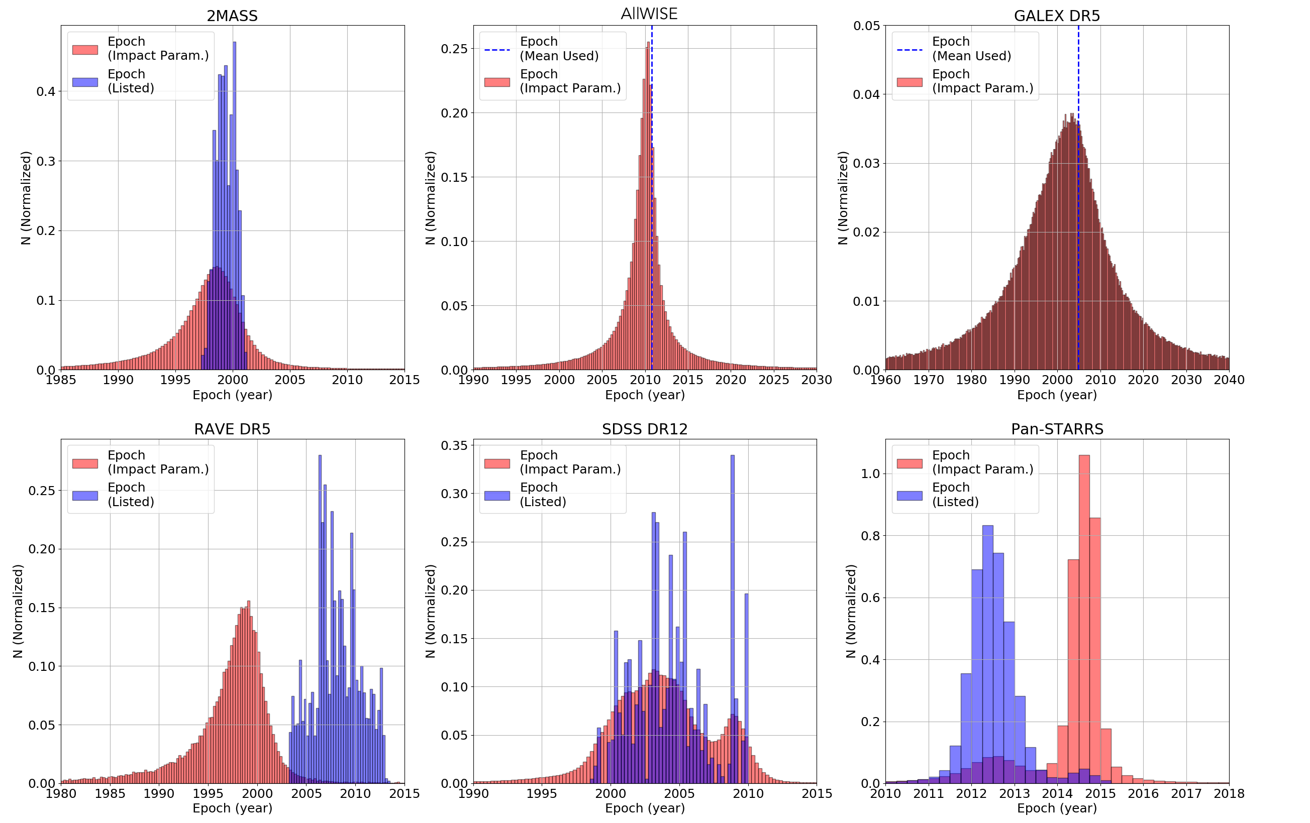
As a check, we examine the distribution of optimal epochs for all the cross-matches from each external catalog; these are shown in Figure 1. We use these distributions to verify the effective mean epoch of each of the external catalogs. Sources with best epochs equal to 1950 or 2050 (the edges of the epoch grid) are excluded as they are unlikely to be correct matches. The widths of the optimal epoch distributions are generally consistent with the astrometric precision of each external catalog, where catalogs like GALEX DR5 demonstrate a much lower angular resolution than a catalog like Pan-STARRS. Additionally, differences between the means of the optimal and listed epoch distributions are indicative of systematic errors in sky coordinates. Whereas catalogs like 2MASS and SDSS DR12 demonstrate relativity small offsets, catalogs like RAVE DR5 and Pan-STARRS show large systematics. Differences in the RAVE DR5 epochs are simply due to the positions of the sources being listed at their 2000.0 epoch and not at the epoch of the spectroscopic observations, which is the value listed in the RAVE catalog. The Pan-STARRS difference, on the other hand, may indicate larger errors in the catalog itself.

Finally, the angular separations of the stars that pass the final cut in the initial search at these mean epochs are calculated and will be used in the subsequent Bayesian analysis.

Figure 1: Distributions for optimal epochs (red histograms) as compared to the listed epochs (blue histograms) for matches with minimzed angular separations between the external source and the Gaia source. For external catalogs that do not list individual epochs for each source (AllWISE and GALEX DR5), the mean epoch assumed for the survey is shown as a blue dotted line.

3.3 Displaced Sample

All sources from an external catalog passing the final angular separation cut are considered possible matches to a specific Gaia source. However, at least some of these matches are bound to be random field stars instead of true counterparts. In order to to evaluate the likelihood that a source is a random field star, we create a “displaced” sample of sources from each external catalog, which is meant to represent a sample of purely random field stars.

This displaced sample is created by repeating the procedure in Sections 3.1 and 3.2, but by first displacing all the Gaia declinations by $\pm 2$ arcminutes (depending if the source is in the northern or southern hemisphere). This creates an initial catalog of cross-matched objects consisting of solely random field stars. Due to the small shift in declination, the field density of the displaced sample is in most cases statistically comparable to the field density of the actual sample used in the cross-match (Lépine & Bongiorno, 2007). When correcting all sources in the displaced sample to a mean epoch, the mean epoch from the true distribution is used to determine the angular separations used in the subsequent Bayesian analysis.

3.4 Bayesian Analysis

Generally, for some vector of observations, $\vec{x}$, the probability of some hypothesis $H_{1}$ given that $\vec{x}$ is true is given by:

$$P(H_{1}|\vec{x})=\frac{P(\vec{x}|H_{1})P(H_{1})}{P(\vec{x})}$$ (8)

Given an alternative hypothesis to $H_{1}$, $H_{0}$, where $P(H_{1})+P(H_{0})=1$, the above expression can be rewritten as:

$$P(H_{1}|\vec{x})=\frac{P(\vec{x}|H_{1})P(H_{1})}{P(\vec{x}|H_{1})P(H_{1})+P(\vec{x}|H_{0})P(H_{0})}$$ (9)

For a cross-match, the initial hypothesis, $H_{1}$, is that the external catalog entry is a match to the Gaia source being considered, or associated with the Gaia source, while the alternate hypothesis, $H_{0}$, is that the external catalog entry is a random field star unrelated to the Gaia source. We include the caveat of “associated with the Gaia source” in the statement for the hypothesis $H_{1}$ to account for any image or pipeline artifact associated with the Gaia source or a possible binary star companion to the Gaia source, as these would not be present in the displaced sample. We do expect that these artifacts/companions will be lower probability, secondary matches in the final result. All Bayesian probabilities in general will be a function of the mean angular separation of the external source, but also of the magnitude of the external source, the $G$ magnitude of the Gaia source, the Galactic latitude of the Gaia source being matched, and possibly other parameters.

In order to increase the dimensionality of the problem, while keeping the probability distributions reasonably simple (e.g. two-dimensions), we will build statistics for different subsets defined by various cuts in e.g. the $G$ magnitude and Galactic latitude of the Gaia source, and reduce the dimensions of the probability distributions to two factors: angular separation, and difference between the external catalog magnitude and the Gaia source $G$ magnitude, or “quasi-color”. The quasi-color parameter will act a spectral type check when paired with examining probability distributions in finite bins of $G$ magnitude, as we would expect the true matches of similar spectral type to center around a determined value in this quasi-color space. For this study, the following bins in Gaia magnitude $G$ and Galactic latitude b are used: $G<10$, $10\leq G<12.5$, $12.5\leq G<15$, $15\leq G<17.5$, $17.5\leq G<20$ and $G\geq 20$, and $|b|<19.5$, $19.5\leq|b|<41.8$ and $|b|\geq 41.8$. The latitude cuts are chosen such that that they cover regions of approximately equal solid angle on the sky. Due to low number statistics, however, these cuts were not applied to the RAVE DR5 sample.

Based on these inputs, the probability of the possible match being a random field star, $P(\vec{x}|H_{0})$, can be directly inferred from the results of the cross match with the displaced sample. This is done by creating a two-dimensional frequency distribution with the displaced sample results for each of the surveys using the same cuts in $G$ and b above.

Frequency distributions are also determined for stars in the true sample, but, as mentioned, these distributions are contaminated by the presence of random field stars. In order to account for the components of the distribution due to these random field stars, the frequency distributions of the displaced samples are used. Under ideal circumstances, the number of random field stars should be the same in both samples, and simple subtraction of the two distributions should suffice in inferring the component of the distribution for the true cross-match that is equivalent to $P(\vec{x}|H_{1})$.

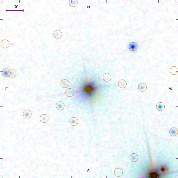
This is not necessarily the case for our distributions though. When performing the search for the displaced sample, all pointings are randomized and are most likely not falling in the immediate vicinity of a bright source. This is however not the case for the true cross-match, since many of the $Gaia$ sources are matched with bright sources in these external catalogs. In these cases, the PSFs of these bright sources outshines some of these random field stars and leaves them missing from the catalog and from our inferred statistical distribution. This “blind spot” effect can be seen in Figure 2, which shows an SDSS image made using the SDSS DR12 Image Tool. In this image, the PSF effectively extends nearly 10 arcseconds from the center of the object. This effect is present in all external catalogs and has an obvious effect on the frequency distributions for the true cross-match. An example of the resulting effect is shown in Figure 3, where, when comparing the two distributions, a large gap in dim stars at short angular separations is observed. In Figure 3, the median and 68th percentile of $W1-G$ as a function of $\theta$ is shown, where quantiles are found using COBS (Ng & Maechler, 2015). These quantiles demonstrate that only at very large angular separations does the distribution of the true sample begin to match that of the displaced sample due to this “outshining” effect.

Figure 2: SDSS image of the source SDSS J000000.21+091332.1 (centered onthe crosshairs), which is matched with Gaia source 2747168838957855104. The orange circles in the image indicate other photometric objects in the SDSS DR12 catalog.

Figure 3: Figure showing the 2D distributions of $W1-G$ color versus angular separation for the AllWISE initial cross match (left panel) and for the displaced sample (right panel), in both cases for Gaia sources with $12.5<G\leq 15$ and $|b|\geq 41.8$. The colormap of the distribution shows the number density of sources in a bin, on a logarithmic scale; both panels have the same colormap range. The median and 68th percentile of $W1-G$ as a function of $\theta$ are shown as the red solid and red dashed lines, respectively, where quantiles are found using COBS (Ng & Maechler, 2015). At small angular separations, the distribution in the left panel is dominated by the counterparts and artifacts/companions in the external catalog, while at larger angular separations the distribution is due to random field stars.

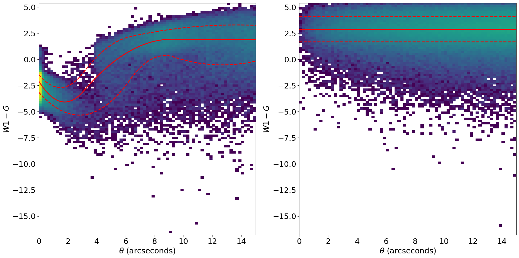
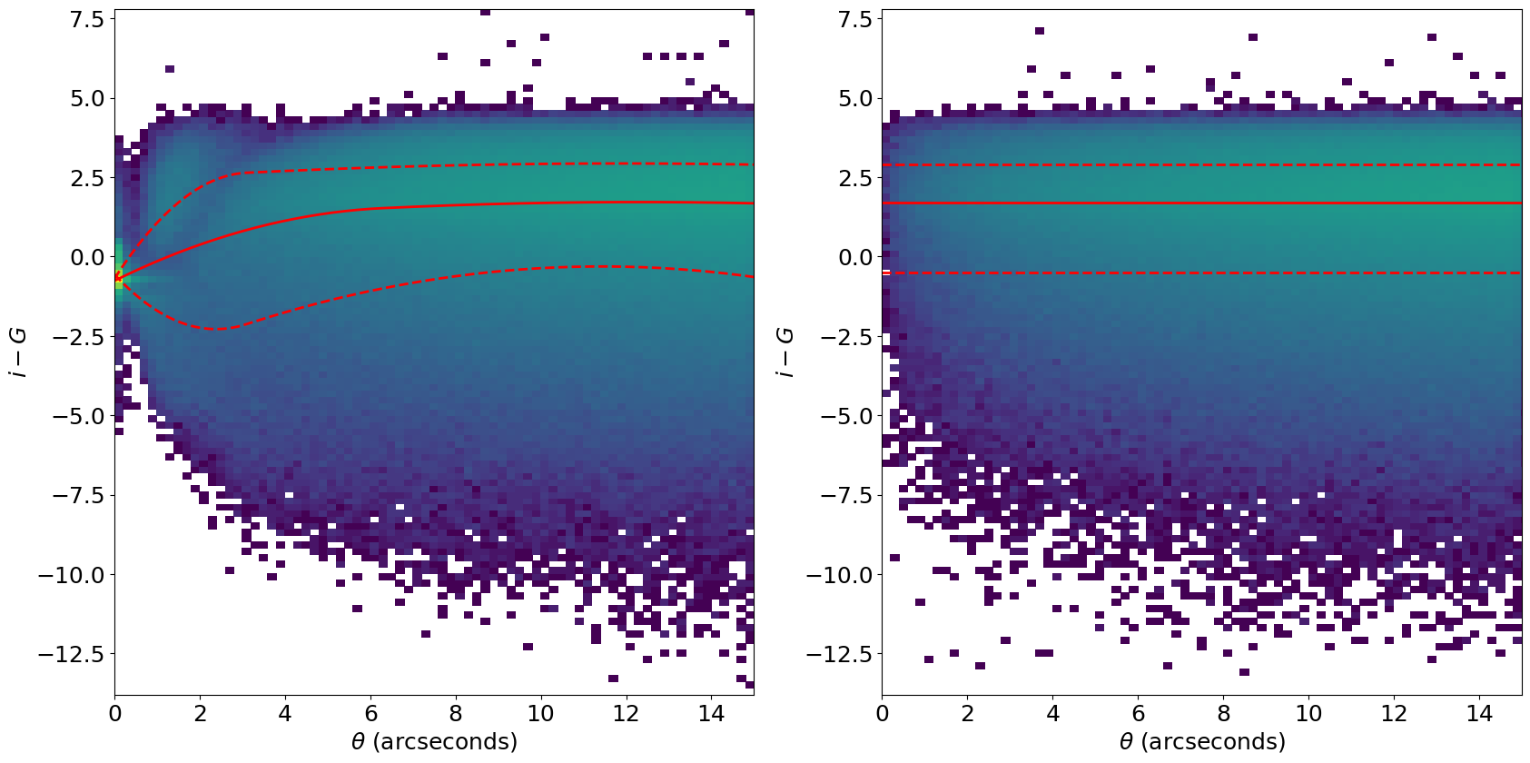
For distributions in bins of fainter $G$ magnitude however, the component due to random field stars in the true distribution becomes more apparent at smaller angular separations as compared to distributions for bright sources (Figure 4). This is seen clearly when comparing the quantiles of the two distributions in Figure 4. It is at these larger angular separations that the displaced distribution is used to model the random field star component. For the brighter bins though, the “outshining” effect discussed above and random fluctuations in the number of random field stars, this distribution at larger angular separations does not always have the same amplitude.

Figure 4: Figure showing the 2D distributions of $i-G$ color versus angular separation for the Pan-STARRS initial cross match (left panel) and for the displaced sample (right panel), in both cases for Gaia sources with $17.5<G\leq 20$ and $19.5\leq|b|<41.8$. The colormap of the distribution shows the number density of sources in a bin, on a logarithmic scale; both panels have the same colormap range. The median and 68th percentile of $i-G$ as a function of $\theta$ are shown as the red solid and red dashed lines, respectively, where quantiles are found using COBS (Ng & Maechler, 2015). At small angular separations, the distribution in the left panel is dominated by the counterparts and artifacts/companions in the external catalog, while at larger angular separations the distribution is due to random field stars.

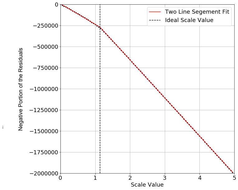
To determine the correct scaling factor and properly subtract the distribution of field stars represented by the displaced sample, we examine the negative part of the residuals. Figure 5 shows the integral of the negative part of the residuals of the inferred frequency distribution for the hypothesis $H_{1}$ after subtracting the frequency distribution of the displaced sample multiplied by a scaling factor. The curve always shows two segments with differing slopes. This change in slope occurs at the point where the scaling factor over-estimates the number of stars in the displaced sample that may have been masked by the PSF of the source in the true sample, causing an over-subtraction to occur. The appropriate scale factor for each distribution, then, is found at the scaling factor where this slope change occurs. We find that this value is usually around $1.0$, where deviations from $1.0$ are due to two reasons. First, deviations from $S=1.0$ can be attributed to random fluctuations in the number of random field stars in both the true and displaced samples. Second, deviations are observed for brighter sources with extended PSFs where the scaling factor is increased to account for the field stars hidden by the PSF.

Figure 5: Plot of the integral of the negative part of the residuals between the true and displaced distribution functions (see eq. 10), represented as black dots. The example above is for a cross-match of our Gaia subset with the Pan-STARRS catalog, with $12.5\leq G<15$ and $19.5\leq|b|<41.8$. The black dashed line shows the intersect of the two model line segments (red lines), which is determined to be the ideal scaling factor for the displaced sample in this region.

In summary, the frequency distribution for the hypothesis $H_{1}$ for a distribution based on some magnitude, $m$, some cut in Gaia $G$ and some cut in Galactic Latitude, b, is given by:

$$F(\vec{x}|H_{1})_{m,G,b}=\begin{cases}f=F(\vec{x}|H_{1}\cup H_{0})_{m,G,b}-S_{m,G,b}\times F(\vec{x}|H_{0})_{m,G,b},&\text{if $f>0$}\\ 0,&\text{if $f\leq 0$}\end{cases}$$ (10)

where $S$ is the scale factor determined from above. The conditional probabilities for a distribution of $m-G$ vs. $\theta$ based on some magnitude, $m$, some cut in Gaia $G$ and some cut in Galactic Latitude, b, are then given by the likelihoods:

$$P(\vec{x}|H_{1})_{m,G,b}=\frac{F(\vec{x}|H_{1})_{m,G,b}}{\sum_{\vec{x}=(\theta,m-G)}F(\vec{x}|H_{1})_{m,G,b}}$$ (11)

$$P(\vec{x}|H_{0})_{m,G,b}=\frac{F(\vec{x}|H_{0})_{m,G,b}}{\sum_{\vec{x}=(\theta,m-G)}F(\vec{x}|H_{0})_{m,G,b}}$$ (12)

Finally, the prior probabilities are based on the expected number of matches and random field stars:

$$P(H_{1})_{m,G,b}=\frac{\sum_{\vec{x}=(\theta,m-G)}F(\vec{x}|H_{1})_{m,G,b}}{\sum_{\vec{x}=(\theta,m-G)}F(\vec{x}|H_{1}\cup H_{0})_{m,G,b}}$$ (13)

$$P(H_{0})_{m,G,b}=1-P(H_{1})_{m,G,b}$$ (14)

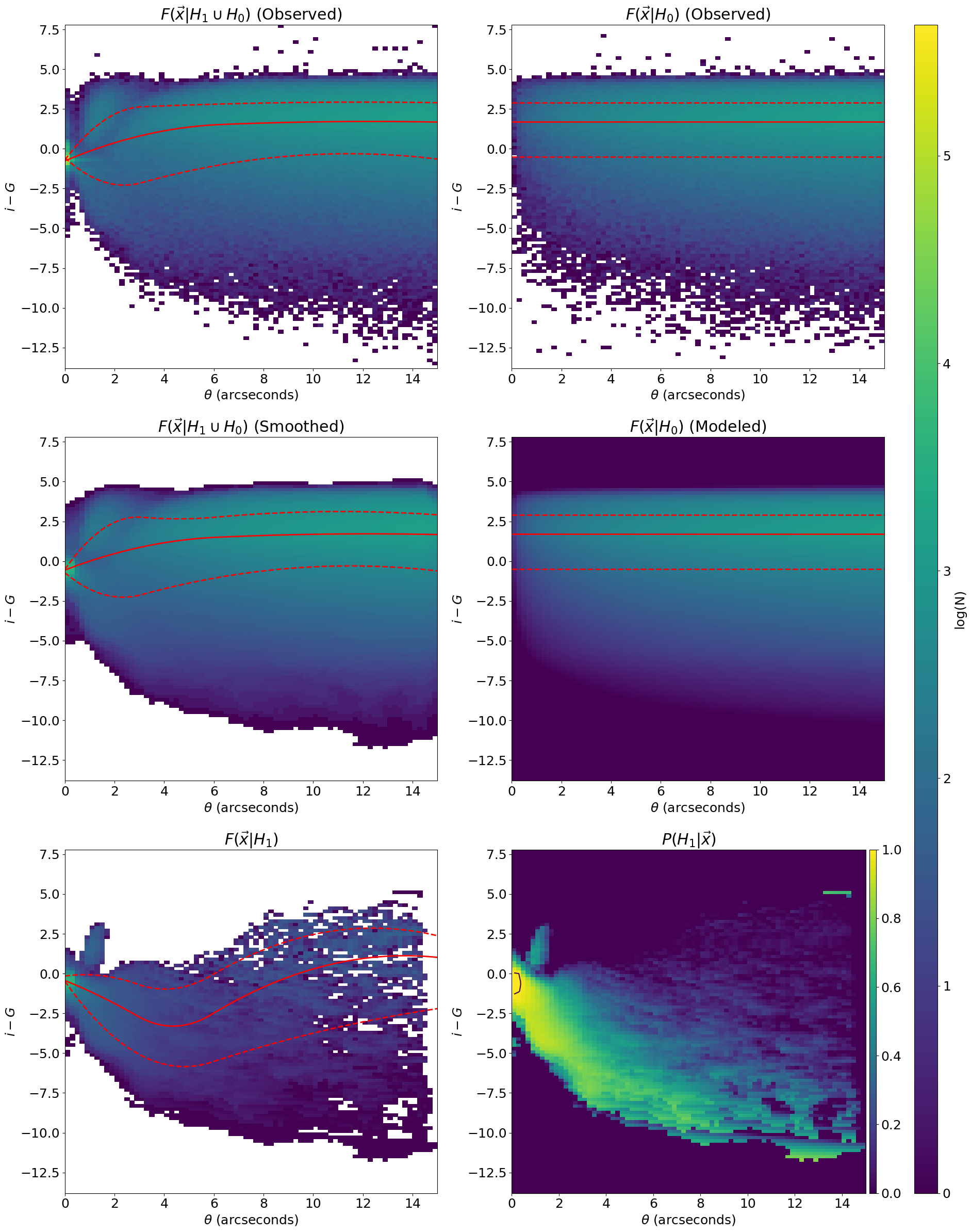
Using the definitions laid out in this section, we can now determine a discrete 2D Bayesian probability distribution based on eq. 9 for all combinations of our $G$ magnitude and Galactic latitude bins, and for every external catalog that we match. An example of the various cross-match distributions discussed above are shown in Figure 6, where the labels above each panel match the functional definitions outlined in eq. 9 and eqs. 11-14. In the bottom right panel of Figure 6, some artifacts are present, such as the line around $(\theta,i-G)\approx(14,5)$. Such artifacts are caused by the smoothing of the true distribution, which can cause an overestimation around the edges of the distribution. When you pair this overestimation along the edge with the lower number of field stars in the displaced model, sometimes these artifacts will arise in the probability distribution. These artificial probabilities are much lower than the best match threshold we use for this study though, so it will not affect the final results.

Figure 6: Cross-match frequency distributions discussed in Section 3.4 for Pan-STARRS counterparts of Gaia with $17.5<G\leq 20$ and $19.5\leq|b|<41.8$. The description of individual panels is as follows: upper left is the frequency distribution for the “true” sample, upper right is the frequency distribution for the “displaced sample”, middle left is the smoothed frequency distribution for the “true” sample, middle right is the modeled frequency distribution for the “displaced” sample, lower left is the difference between the smoothed “true” frequency distribution and the modeled “displaced” frequency distribution using the correct scaling factor, and the lower right is the resulting Bayesian probability distribution. All plots, except for the distribution for $P(H_{1}|\vec{x})$, show the number of sources per bin on a logarithmic scale and they all share the same colormap range (indicated by the colorbar on the far right). The median and 68th percentile of $i-G$ as a function of $\theta$ are shown on these plots as the red solid and red dashed lines, respectively, where quantiles are found using COBS (Ng & Maechler, 2015). The distribution for $P(H_{1}|\vec{x})$ is shown for a range of 0 to 1 and the black solid line overlaid shows the 99% line.

3.5 Distribution Smoothing and Modeling

One of the issues with the above procedure is the statistical noise present in these distributions. To remedy this, while keeping relatively small bin sizes for the frequency distributions, a percentile smoothing filter was applied and the priors of the discrete and smoothed distributions are then found to be comparable.

Another issue with the procedure is that in low occurrence regimes, the under-sampling of the displaced sample distribution can cause artificially high Bayesian probabilities. Fortunately, while the true cross-match distribution is too complex to model in most cases, the displaced sample distribution is fairly easily modeled. This is because the placement of fields stars is inherently random, and the angular separation and magnitudes differences can be considered independent variables, and their distributions modeled separately.

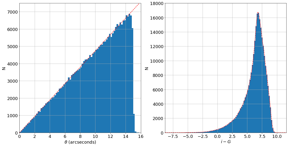
Representative models of these one-dimensional, independent distributions are shown in Figure 7. As can be seen from the left panel, the angular separations form a distribution that increases linearly at higher separations:

$$F(x=\theta)=mx+b$$ (15)

The quasi-color distribution (right panel), on the other hand, can be modeled as a sum of normal distributions with varying weights:

$$F(y=m-G)=\sum_{i}^{n}W_{i}e^{-\frac{(y-\mu_{i})^{2}}{2\sigma_{i}^{2}}}$$ (16)

The number of components is varied from $n=2$ to $n=10$, and the ideal number of components is based on the function that minimizes the Bayesian information criterion (BIC):

$$\text{BIC}=n\ ln\left[\frac{\sum(F(x)_{measured}-F(x)_{model})^{2}}{n}\right]+k\ ln(n)$$ (17)

Where $n$ is the number of data points used for the model and $k$ is the number of components.

Figure 7: 1D distributions (blue bins) of angular separation (left panel) and $i-G$ (right panel) for cross-matched pairs in the Pan-STARRS displaced sample with $12.5\leq G<15$ and $19.5\leq|b|<41.8$. The best models based on eqs. 15 and 16 are shown as the red dashed lines.

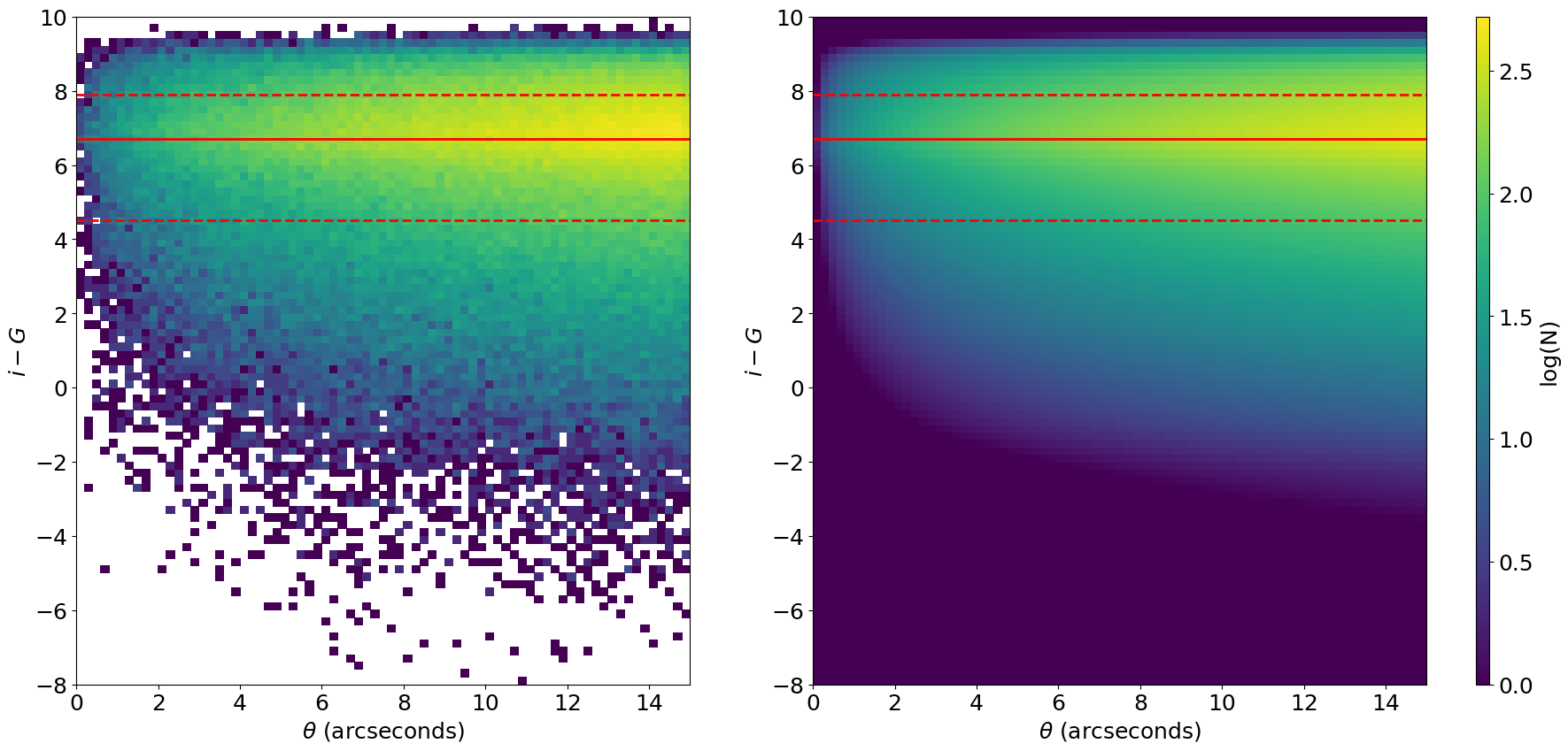
After fitting the above equations to the 1D distributions for each of the displaced samples, the 2D distribution of field stars from the displaced sample can generally be modeled by:

$$F(\vec{x}|H_{0})=F(x=\theta,y=m-G)=C(mx+b)\sum_{i}^{n}W_{i}e^{-\frac{(y-\mu_{i})^{2}}{2\sigma_{i}^{2}}}$$ (18)

where the scaling constant $C$ is added to ensure the scale of the modeled distribution matches that of the observed distribution. Best-fitting parameters are evaluated separately for each distribution; one example is shown on the right panel in Figure 8, where it is compared to its associated observed distribution on the left. As a note, this modelling procedure is completed for 18 different distributions per photometric band in each survey, to account for all combinations of Gaia $G$ and Galactic latitude bins described in Section 3.4, so the parameters in eq. 18 will be different for each of these distributions.

Figure 8: 2D distributions of $i-G$ versus angular separation for the Pan-STARRS displaced sample with $12.5\leq G<15$ and $19.5\leq|b|<41.8$. The colormap of the distribution shows the number of sources in a bin on a logarithmic scale and both panels have the same colormap range. The left panel shows the observed displaced distribution while the right panel shows the modeled distribution. Additionally, the median and 68th percentile of $i-G$ as a function of $\theta$ are shown as the red solid and red dashed lines, respectively, where quantiles are found using COBS (Ng & Maechler, 2015).

3.6 High Probability Matches

In order to determine the best matches from the external catalogs to the Gaia sources, we calculate the total probability defined as the product of the probabilities for each magnitude in a given catalog, when there is a valid magnitude measurement for the source. For SDSS DR12 sources not part of the primary catalog (i.e. are flagged as duplicates in the SDSS DR12) we force their probability to be 0%. It should be noted that this does imply that for catalogs with a larger number of photometric measurements, the individual probabilities must be higher to reach this $95\%$ threshold. For example, for a catalog like 2MASS that has three photometric measurements, each individual magnitude must have a probability $>98.30\%$ on average to reach the $95\%$ threshold, while a catalog like Pan-STARRS that has five photometric measurements would require each individual magnitude to have a probability $>98.98\%$ on average. This small difference should not cause a large difference in the final catalog of high probability matches as a large number of the stars with high probability have probabilities $>99\%$ (see black line in lower right panel of Figure 6). Best matches are then defined as those possible sources with a total probability $>95\%$, and if multiple entries in a catalog have a total probability $>95\%$ for a particular Gaia source the catalog entry with the largest total probability is designated as the best match. Table 1 shows the percentage of matches to Gaia sources that meet this criterion. Low match percentages for catalogs like SDSS DR12 and Pan-STARRS can be attributed to the difference in sky coverage, while low match probabilities in the other catalogs can be attributed to the limiting magnitudes of the external catalogs.

Table 1: Number of sources matched with a total probability $>95\%$

External Catalog	% Matched
2MASS	75.40%
AllWISE	75.17%
GALEX DR5	8.36%
RAVE DR5	0.63%
SDSS DR12	30.69%
Pan-STARRS	68.63%

The catalog of “best matches”, i.e. where the Gaia sources have a counterpart with total probability $>95\%$, is presented in Table 2. As a supplement, Tables 3-8 give all possible matches for each of the cross matches such that the user can vary the tolerances and obtain alternate and/or additional matches to the Gaia sources. The code needed to reproduce these results, or perform additional cross-matches, can also be found on our GitHub repository.

Table 2: Best matches found in this study with a Bayesian probability greater than 95% for all cross matches in this study.

Column Number	Label	Units	Column Description
1	GaiaDR2_ID	$\cdots$	Gaia DR2 Identifier
2	Gmag_GaiaDR2	mag	Gaia DR2 G-band magnitude
3	BPmag_GaiaDR2	mag	Gaia DR2 BP-band magnitude
4	RPmag_GaiaDR2	mag	Gaia DR2 RP-band magnitude
5	RA_ICRS_GaiaDR2	deg	Right ascension at Epoch=2015.5 from Gaia DR2
6	DE_ICRS_GaiaDR2	deg	Declination at Epoch=2015.5 from Gaia DR2
7	PLX_GaiaDR2	mas	Parallax measurment from Gaia DR2
8	PLXerr_GaiaDR2	mas	Parallax measurment error from Gaia DR2
9	PMRA_GaiaDR2	mas/yr	Proper motion in right ascension direction (PMRA*cosDE) from Gaia DR2
10	PMDE_GaiaDR2	mas/yr	Proper motion in declination direction from Gaia DR2
11	SDSSDR12_ID	$\cdots$	SDSS DR12 Identifier
12	umag_SDSSDR12	mag	u-band magntiude on AB scale from SDSS DR12
13	umag_err_SDSSDR12	mag	u-band magntiude error on AB scale from from SDSS DR12
14	gmag_SDSSDR12	mag	g-band magntiude on AB scale from from SDSS DR12
15	gmag_err_SDSSDR12	mag	g-band magntiude error on AB scale from from SDSS DR12
16	rmag_SDSSDR12	mag	r-band magntiude on AB scale from from SDSS DR12
17	rmag_err_SDSSDR12	mag	r-band magntiude error on AB scale from from SDSS DR12
18	imag_SDSSDR12	mag	i-band magntiude on AB scale from from SDSS DR12
19	imag_err_SDSSDR12	mag	i-band magntiude error on AB scale from from SDSS DR12
20	zmag_SDSSDR12	mag	z-band magntiude on AB scale from from SDSS DR12
21	zmag_err_SDSSDR12	mag	z-band magntiude error on AB scale from from SDSS DR12
22	RA_ICRS_SDSSDR12	deg	Right ascension from SDSS DR12 (ICRS)
23	DE_ICRS_SDSSDR12	deg	Declination from SDSS DR12 (ICRS)
24	Bayes_Prob_SDSSDR12	$\cdots$	Total bayesian probability of SDSS DR12 object match to Gaia DR2 Object
25	Ang_Sep_SDSSDR12	arcsec	Angular separation between SDSS DR12 object and Gaia DR2 object at mean epoch of SDSS DR12
26	2MASS_ID	$\cdots$	2MASS Identifier
27	Jmag_2MASS	mag	J-band magntiude from 2MASS
28	Jmag_err_2MASS	mag	J-band magntiude error from 2MASS
29	Hmag_2MASS	mag	H-band magntiude from 2MASS
30	Hmag_err_2MASS	mag	H-band magntiude error from 2MASS
31	Ksmag_2MASS	mag	Ks-band magntiude from 2MASS
32	Ksmag_err_2MASS	mag	Ks-band magntiude error from 2MASS
33	RA_J2000_2MASS	deg	Right ascension from 2MASS (J2000)
34	DE_J2000_2MASS	deg	Declination from 2MASS (J2000)
35	Bayes_Prob_2MASS	$\cdots$	Total bayesian probability of 2MASS object match to Gaia DR2 Object
36	Ang_Sep_2MASS	arcsec	Angular separation between 2MASS object and Gaia DR2 object at mean epoch of 2MASS
37	AllWISE_ID	$\cdots$	AllWISE Identifier
38	W1mag_AllWISE	mag	W1-band magnitude from AllWISE
39	W1mag_err_AllWISE	mag	W1-band magntiude error from AllWISE
40	W2mag_AllWISE	mag	W2-band magnitude from AllWISE
41	W2mag_err_AllWISE	mag	W2-band magntiude error from AllWISE
42	W3mag_AllWISE	mag	W3-band magnitude from AllWISE
43	W3mag_err_AllWISE	mag	W3-band magntiude error from AllWISE
44	W4mag_AllWISE	mag	W4-band magnitude from AllWISE
45	W4mag_err_AllWISE	mag	W4-band magntiude error from AllWISE
46	RA_J2000_AllWISE	deg	Right ascension from AllWISE (J2000)
47	DE_J2000_AllWISE	deg	Declination from AllWISE (J2000)
48	Bayes_Prob_AllWISE	$\cdots$	Total bayesian probability of AllWISE object match to Gaia DR2 Object
49	Ang_Sep_AllWISE	arcsec	Angular separation between AllWISE object and Gaia DR2 object at mean epoch of AllWISE
50	GALEXDR5_ID	$\cdots$	GALEX DR5 Identifier
51	FUVmag_GALEXDR5	mag	FUV-band magnitufe from GALEX DR5
52	FUVmag_err_GALEXDR5	mag	FUV-band magntiude error from GALEX DR5
53	NUVmag_GALEXDR5	mag	NUV-band magnitufe from GALEX DR5
54	NUVmag_err_GALEXDR5	mag	NUV-band magntiude error from GALEX DR5
55	RA_J2000_GALEXDR5	deg	Right ascension from GALEX DR5 (J2000)
56	DE_J2000_GALEXDR5	deg	Declination from GALEX DR5 (J2000)
57	Bayes_Prob_GALEXDR5	$\cdots$	Total bayesian probability of GALEX DR5 object match to Gaia DR2 Object
58	Ang_Sep_GALEXDR5	arcsec	Angular separation between GALEX DR5 object and Gaia DR2 object at mean epoch of GALEX DR5
59	PS1_ID	$\cdots$	Pan-STARRS Identifier
60	gmag_PS1	mag	g-band magntiude on AB scale from Pan-STARRS
61	gmag_err_PS1	mag	g-band magntiude error on AB scale from Pan-STARRS
62	rmag_PS1	mag	r-band magntiude on AB scale from Pan-STARRS
63	rmag_err_PS1	mag	r-band magntiude error on AB scale from Pan-STARRS
64	imag_PS1	mag	i-band magntiude on AB scale from Pan-STARRS
65	imag_err_PS1	mag	i-band magntiude error on AB scale from Pan-STARRS
66	zmag_PS1	mag	z-band magntiude on AB scale from Pan-STARRS
67	zmag_err_PS1	mag	z-band magntiude error on AB scale from Pan-STARRS
68	ymag_PS1	mag	y-band magntiude on AB scale from Pan-STARRS
69	ymag_err_PS1	mag	y-band magntiude error on AB scale from Pan-STARRS
70	RA_J2000_PS1	deg	Right Ascension from Pan-STARRS (J2000)
71	DE_J2000_PS1	deg	Declination from Pan-STARRS (J2000)
72	Bayes_Prob_PS1	$\cdots$	Total bayesian probability of Pan-STARRS object match to Gaia DR2 Object
73	Ang_Sep_PS1	arcsec	Angular separation between Pan-STARRS object and Gaia DR2 object at mean epoch of Pan-STARRS
74	RAVEDR5_ID	$\cdots$	RAVE DR5 Identifier
75	BTmag_RAVEDR5	mag	Tycho-2 BT magnitude listed in RAVE DR5
76	BTmag_err_RAVEDR5	mag	Tycho-2 BT magnitude error listed in RAVE DR5
77	VTmag_RAVEDR5	mag	Tycho-2 VT magnitude listed in RAVE DR5
78	VTmag_err_RAVEDR5	mag	Tycho-2 VT magnitude error listed in RAVE DR5
79	RA_J2000_RAVEDR5	deg	Right ascension fr0m RAVE DR5 (J2000)
80	DE_J2000_RAVEDR5	deg	Declination from RAVE DR5 (J2000)
81	Bayes_Prob_RAVEDR5	$\cdots$	Total bayesian probability of RAVE DR5 object match to Gaia DR2 Object
82	Ang_Sep_RAVEDR5	arcsec	Angular separation between RAVE DR5 object and Gaia DR2 object at mean epoch of RAVE DR5

Note. — This table is published in its entirety in the machine-readable format in the electric version of this manuscript. The description of its columns are shown here for guidance regarding its form and content.

Table 3: All of the possible matches for the cross match between Gaia and 2MASS. For more detailed descriptions of the columns in this table, look at the corresponding columns in Table 2.

Gaia ID	G	$\alpha_{Gaia}$	$\delta_{Gaia}$	2MASS ID	$J$	$\sigma_{J}$	$H$	$\sigma_{H}$	$K$	$\sigma_{K}$	$\alpha_{2MASS}$	$\delta_{2MASS}$	Bayes Prob.	$\Delta\theta$
	[mag]	[deg]	[deg]		[mag]	[mag]	[mag]	[mag]	[mag]	[mag]	[deg]	[deg]		[arcsec]
429379051804727296	16.9667	0.00021864741	60.89771179398	00000009+6053531	13.876	0.024	13.308	0.032	13.055	0.026	0.00039	60.898087	0.9993495	0.1131188
429379051804727296	16.9667	0.00021864741	60.89771179398	00000116+6054047	16.228	0.1	15.771	0.156	15.436	0.195	0.004842	60.901306	0.0	13.893606
384318827606840448	17.9638	0.00047931984	42.19465632646	00000004+4211408	14.897	0.038	14.253	0.045	13.992	0.051	0.000202	42.194679	0.9998343	0.0210179
2772104109112208256	18.4284	0.00051294158	15.565175017629997	00000015+1533550	15.539	0.061	15.081	0.093	14.763	0.0970	0.00065	15.565296	0.999958	0.1038959
4922439138656081024	16.1428	0.00054775339	-57.26154422458	00000021-5715408	13.517	0.025	12.957	0.028	12.713	0.0290	0.000914	-57.261356	0.9999721	0.2605187
2738617902668633344	16.053	0.00059265319	1.41569388809	00000009+0124562	14.005	0.028	13.378	0.029	13.19	0.034	0.00041	1.415625	0.9999895	0.0681481
422597225421620992	19.7116	0.00062329596	57.67086338256	00000006+5740156	16.327	0.119	15.766	0.143	15.057	$\cdots$	0.000289	57.671021	0.9888028	0.2357019
2420684907087327104	16.4742	0.000644395	-14.44069806218	00000012-1426271	14.273	0.032	13.616	0.033	13.47	0.037	0.000518	-14.440871	0.9999867	0.0757191
2305877746911854336	16.9816	0.00064631606	-41.07994573153	00000010-4104482	14.338	0.043	13.627	0.038	13.532	0.045	0.000449	-41.080074	0.9999833	0.1291896
2305877746911854336	16.9816	0.00064631606	-41.07994573153	00000046-4104378	16.126	0.089	15.426	0.111	15.211	0.152	0.00193	-41.07719	0.0744052	11.2620835

Note. — This table is published in its entirety in the machine-readable format. A portion is shown here for guidance regarding its form and content.

=0.65in

Table 4: All of the possible matches for the cross match between Gaia and AllWISE. For more detailed descriptions of the columns in this table, look at the corresponding columns in Table 2.

Gaia ID	G	$\alpha_{Gaia}$	$\delta_{Gaia}$	AllWISE ID	$W1$	$\sigma_{W1}$	$W2$	$\sigma_{W2}$	$W3$	$\sigma_{W3}$	$W4$	$\sigma_{W4}$	$\alpha_{AllWISE}$	$\delta_{AllWISE}$	Bayes Prob.	$\Delta\theta$
	[mag]	[deg]	[deg]		[mag]	[mag]	[mag]	[mag]	[mag]	[mag]	[mag]	[mag]	[deg]	[deg]		[arcsec]
429379051804727296	16.9667	0.00021864741	60.89771179398	J000000.06+605352.1	12.938	0.026	12.789	0.027	12.975	$\cdots$	9.619	$\cdots$	0.0002866	60.8978205	0.9990087	0.0652974
4991418100136496000	16.9943	0.00032430948	-45.44935581167	J000000.05-452657.5	12.97	0.024	12.826	0.026	11.821	$\cdots$	8.402	$\cdots$	0.0002164	-45.4493089	0.0	0.0829052
2314289015157585664	20.407	0.00047449546	-32.67650819595	J000000.10-324035.5	17.812	0.216	17.295	0.493	12.047	$\cdots$	8.683	$\cdots$	0.0004466	-32.6765412	0.995448	0.3449281
384318827606840448	17.9638	0.00047931984	42.19465632646	J000000.09+421140.7	13.882	0.026	13.769	0.032	12.516	$\cdots$	9.007	$\cdots$	0.0003918	42.1946548	0.9994221	0.0253729
2772104109112208256	18.4284	0.00051294158	15.56517501763	J000000.13+153354.8	14.6	0.031	14.366	0.055	12.449	$\cdots$	8.658	$\cdots$	0.0005666	15.5652269	0.9994498	0.0618302
4922439138656081024	16.1428	0.00054775339	-57.26154422458	J000000.16-571541.2	12.651	0.024	12.452	0.023	12.385	$\cdots$	9.173	$\cdots$	0.0006692	-57.2614716	0.9998207	0.0245727
2738617902668633344	16.053	0.00059265319	1.41569388809	J000000.13+012456.4	13.117	0.024	13.174	0.03	11.927	$\cdots$	8.819	$\cdots$	0.0005457	1.4156679	0.9997752	0.0552086
2420684907087327104	16.4742	0.000644395	-14.44069806218	J000000.14-142626.6	13.351	0.023	13.354	0.031	11.984	$\cdots$	8.513	$\cdots$	0.0006046	-14.4407494	0.9994174	0.0174426
2305877746911854336	16.9816	0.00064631606	-41.07994573153	J000000.16-410448.0	13.25	0.024	13.155	0.027	12.562	0.477	9.173	$\cdots$	0.0006781	-41.0800067	0.9993026	0.2645646
2305877746911854336	16.9816	0.00064631606	-41.07994573153	J000000.50-410436.8	15.163	0.052	15.112	0.084	12.574	$\cdots$	9.047	$\cdots$	0.0021152	-41.0768938	0.0	11.915629

Note. — This table is published in its entirety in the machine-readable format. A portion is shown here for guidance regarding its form and content.

Table 5: All of the possible matches for the cross match between Gaia and GALEX DR5. For more detailed descriptions of the columns in this table, look at the corresponding columns in Table 2.

Gaia ID	G	$\alpha_{Gaia}$	$\delta_{Gaia}$	GALEX DR5 ID	$FUV$	$\sigma_{FUV}$	$NUV$	$\sigma_{NUV}$	$\alpha_{GALEX}$	$\delta_{GALEX}$	Bayes Prob.	$\Delta\theta$
	[mag]	[deg]	[deg]		[mag]	[mag]	[mag]	[mag]	[deg]	[deg]		[arcsec]
4991418100136496000	16.9943	0.00032430948	-45.44935581167	6384813650104815341	$\cdots$	$\cdots$	22.495	0.464	0.005075	-45.448452	0.2391745	13.0376701
2747168838957855104	12.9883	0.00100436367	9.22566353979	6376052767224496578	$\cdots$	$\cdots$	18.421	0.058	0.00088	9.225952	0.9999961	1.0644309
2739983083793578368	12.7572	0.00113295198	3.02061233516	6381013735771736390	$\cdots$	$\cdots$	18.946	0.077	0.001213	3.020992	0.9999957	0.5896474
4976553527564650496	16.0853	0.00113599787	-50.7069141397	6384813684464554035	$\cdots$	$\cdots$	21.502	0.22	0.000586	-50.706711	0.9997666	0.7214425
2422910181182822784	13.6938	0.00181091004	-9.91118104462	6380415555275327592	$\cdots$	$\cdots$	22.407	0.49	0.001584	-9.910674	0.9993253	1.510795
2341416475275983872	14.3727	0.00212583048	-21.25877753606	6380556326049682051	$\cdots$	$\cdots$	23.007	0.399	0.000507	-21.260026	0.0	6.5963465
4702977442386044032	16.3353	0.00371708969	-70.18979943279	6384884009185313203	$\cdots$	$\cdots$	21.812	0.28	0.003073	-70.189192	0.9945253	1.9620924
2875011834762675200	20.2727	0.00390831131	33.17729257174	6376756383799313130	$\cdots$	$\cdots$	22.337	0.463	0.005806	33.180352	0.0	11.9387993
2341335283213230464	10.9516	0.00419603514	-21.68609418402	6380556326051776169	20.541	0.116	14.589	0.004	0.004004	-21.686302	1.0000001	0.3253531
2335082979062194304	16.9159	0.00480314620	-25.16797866075	6380556367925610339	$\cdots$	$\cdots$	21.476	0.347	0.004921	-25.167562	0.9998403	0.8272201

Note. — This table is published in its entirety in the machine-readable format. A portion is shown here for guidance regarding its form and content.

=0.7in

Table 6: All of the possible matches for the cross match between Gaia and Pan-STARRS. For more detailed descriptions of the columns in this table, look at the corresponding columns in Table 2.

Gaia ID	G	$\alpha_{Gaia}$	$\delta_{Gaia}$	Pan-STARRS ID	$g$	$\sigma_{g}$	$r$	$\sigma_{r}$	$i$	$\sigma_{i}$	$z$	$\sigma_{z}$	$y$	$\sigma_{y}$	$\alpha_{PS1}$	$\delta_{PS1}$	Bayes Prob.	$\Delta\theta$
	[mag]	[deg]	[deg]		[mag]	[mag]	[mag]	[mag]	[mag]	[mag]	[mag]	[mag]	[mag]	[mag]	[deg]	[deg]		[arcsec]
429379051804727296	16.9667	0.00021864741	60.89771179398	181070000002178144	18.9908	0.0032	17.7993	0.0042	16.2296	0.0028	15.5105	0.0014	15.1478	0.0045	0.00022122	60.89773213	0.9960894	0.0443499
429379051804727296	16.9667	0.00021864741	60.89771179398	181070000017386176	$\cdots$	$\cdots$	$\cdots$	$\cdots$	21.503	0.1446	20.7487	0.1538	$\cdots$	$\cdots$	0.00180374	60.89620386	0.0188694	6.1896178
429379051804727296	16.9667	0.00021864741	60.89771179398	181070000029977216	$\cdots$	$\cdots$	$\cdots$	$\cdots$	21.0219	0.0667	20.7423	0.0955	$\cdots$	$\cdots$	0.00298512	60.89703229	0.0159218	5.460592
429379051804727296	16.9667	0.00021864741	60.89771179398	181070000048379136	21.7554	0.2015	20.4099	0.0365	19.7856	0.0142	19.4149	0.0327	19.1697	0.035	0.00481773	60.89865394	0.0	8.6744328
429379051804727296	16.9667	0.00021864741	60.89771179398	181080000049152160	18.8686	0.0183	18.0388	0.0056	17.6127	0.008	17.3777	0.0068	17.1979	0.0084	0.00491942	60.90115514	0.0	14.7724567
2314289015157585664	20.407	0.00047449546	-32.67650819595	68780000004548592	$\cdots$	$\cdots$	$\cdots$	$\cdots$	19.8489	0.0183	$\cdots$	$\cdots$	$\cdots$	$\cdots$	0.00047162	-32.67650276	0.9996824000000001	0.0394867
384318827606840448	17.9638	0.00047931984	42.19465632646	158630000003914240	19.9025	0.0054	18.6328	0.0068	17.2093	0.0023	16.5534	0.0032	16.2281	0.0048	0.00046683	42.19465832	0.99864	0.0246682
2772104109112208256	18.4284	0.00051294158	15.56517501763	126670000005728752	20.2047	0.0216	19.0564	0.0123	17.6737	0.0047	17.0499	0.0045	16.7519	0.0051	0.00052103	15.56518018	0.9995842	0.0219664
2738617902668633344	16.053	0.00059265319	1.41569388809	109690000004829264	17.2422	0.0034	16.0862	0.0039	15.5176	0.0022	15.2649	0.0051	15.0979	0.0055	0.00057851	1.4156878	0.9999516	0.0064351
2738617902668633344	16.053	0.00059265319	1.41569388809	109690000006064288	21.7947	0.2067	21.7223	0.0567	21.5412	0.0293	20.7805	0.1455	$\cdots$	$\cdots$	0.00072035	1.41159149	0.0	14.7581938

Note. — This table is published in its entirety in the machine-readable format. A portion is shown here for guidance regarding its form and content.

=0.7in

Table 7: All of the possible matches for the cross match between Gaia and SDSS DR12. For more detailed descriptions of the columns in this table, look at the corresponding columns in Table 2.

Gaia ID	G	$\alpha_{Gaia}$	$\delta_{Gaia}$	SDSS DR12 ID	$u$	$\sigma_{u}$	$g$	$\sigma_{g}$	$r$	$\sigma_{r}$	$i$	$\sigma_{i}$	$z$	$\sigma_{z}$	$\alpha_{SDSS}$	$\delta_{SDSS}$	Bayes Prob.	$\Delta\theta$
	[mag]	[deg]	[deg]		[mag]	[mag]	[mag]	[mag]	[mag]	[mag]	[mag]	[mag]	[mag]	[mag]	[deg]	[deg]		[arcsec]
2772104109112208256	18.4284	0.00051294158	15.56517501763	J000000.15+153354.9	23.126	0.421	20.441	0.023	19.025	0.011	17.637	0.007	16.912	0.011	0.000635	15.565261	0.9997612	0.0421463
2772104109112208256	18.4284	0.00051294158	15.56517501763	J000000.15+153354.9	22.831	0.297	20.454	0.022	19.048	0.011	17.655	0.007	16.941	0.01	0.000641	15.565276	0.0	0.0975381
2772104109112208256	18.4284	0.00051294158	15.56517501763	J000000.30+153408.3	24.246	0.701	23.369	0.217	22.907	0.201	23.235	0.346	22.838	0.428	0.001256	15.568985	0.0	13.6115789
2772104109112208256	18.4284	0.00051294158	15.56517501763	J000000.30+153408.4	23.284	0.491	23.025	0.176	22.679	0.175	22.568	0.278	23.536	0.605	0.001261	15.569004	0.0	13.6818764
2738617902668633344	16.053	0.00059265319	1.41569388809	J000000.12+012456.3	20.117	0.042	17.428	0.005	16.074	0.004	15.493	0.004	15.171	0.005	0.000531	1.41566	0.9999276	0.2760008
2738617902668633344	16.053	0.00059265319	1.41569388809	J000000.17+012441.5	24.972	1.399	22.099	0.131	21.326	0.092	20.721	0.083	20.653	0.269	0.000739	1.411541	0.0	14.8164078
2873403867726399232	19.0963	0.00089948698	30.80569762321	J000000.17+304820.6	22.965	0.295	20.334	0.018	19.103	0.011	18.554	0.01	18.258	0.024	0.000712	30.805743	0.9997258	0.0623462
2873403867726399232	19.0963	0.00089948698	30.80569762321	J000000.19+304820.5	22.385	0.258	20.356	0.019	19.064	0.011	18.537	0.011	18.21	0.024	0.000833	30.805711	0.0	0.4533442
2747168838957855104	12.9883	0.00100436367	9.22566353979	J000000.21+091332.1	15.214	0.005	14.593	0.005	13.118	0.002	12.915	0.002	13.1	0.005	0.000893	9.225608	0.9999519	0.1975248
2747168838957855104	12.9883	0.00100436367	9.22566353979	J000000.96+091330.2	23.84	1.334	23.15	0.271	22.441	0.257	21.988	0.243	23.428	0.883	0.004033	9.225064	0.0	11.4517712

Note. — This table is published in its entirety in the machine-readable format. A portion is shown here for guidance regarding its form and content.

Table 8: All of the possible matches for the cross match between Gaia and RAVE DR5. For more detailed descriptions of the columns in this table, look at the corresponding columns in Table 2.

Gaia ID	G	$\alpha_{Gaia}$	$\delta_{Gaia}$	RAVE DR5 ID	$B_{T}$	$\sigma_{B_{T}}$	$V_{T}$	$\sigma_{V_{T}}$	$\alpha_{RAVE}$	$\delta_{RAVE}$	Bayes Prob.	$\Delta\theta$
	[mag]	[deg]	[deg]		[mag]	[mag]	[mag]	[mag]	[deg]	[deg]		[arcsec]
4919074289477561472	11.6106	0.00780738967	-58.71847417652	J000001.9-584307	12.533	0.154	11.706	0.103	0.00808	-58.71853	0.9934741	0.2496141
4919427610667433600	16.5728	0.03675557788	-57.48719495688	J000009.0-572913	$\cdots$	$\cdots$	$\cdots$	$\cdots$	0.03729	-57.48683	0.0	2.1838843
4919427610667433728	13.0809	0.03783936489	-57.4868416914	J000009.0-572913	$\cdots$	$\cdots$	$\cdots$	$\cdots$	0.03729	-57.48683	0.0	0.2650074
4973451770902209920	13.2093	0.05450144802	-51.61164961089	J000013.0-513642	$\cdots$	$\cdots$	$\cdots$	$\cdots$	0.05404	-51.61158	0.0	0.2256993
2413944625931002624	12.148	0.06847151987	-19.10762290314	J000016.3-190627	$\cdots$	$\cdots$	$\cdots$	$\cdots$	0.068	-19.10758	0.0	0.2232123
2448187747347233664	11.0992	0.06966855007	-2.94569133915	J000016.7-025652	10.927	0.048	10.002	0.032	0.06971	-2.94781	0.6104921	7.8678634
2448187747347250048	9.7686	0.0698486806	-2.94784184175	J000016.7-025652	10.927	0.048	10.002	0.032	0.06971	-2.94781	0.9946625	0.3243487
4634503362901736576	10.6905	0.07271168199	-80.26747298433	J000017.1-801603	11.828	0.079	11.019	0.069	0.07125	-80.26739	0.9946625	0.1978637
2420804032300281728	12.7836	0.07347788125	-13.57904040546	J000017.7-133444	$\cdots$	$\cdots$	$\cdots$	$\cdots$	0.07354	-13.57889	0.0	0.2641875
2414164459536733952	9.9923	0.0744390513	-18.17238322596	J000017.7-181021	11.006	0.046	10.204	0.033	0.07392	-18.1725	0.9946625	0.045774

Note. — This table is published in its entirety in the machine-readable format. A portion is shown here for guidance regarding its form and content.

4 Photometric Metallicity Determination

With the cross-matched data discussed above, we can now assemble a catalog of stars that includes not only a large variety of photometric bands for all objects, but also spectra for a subset of $\sim$21,000 stars thanks to surveys like SDSS. Using the derived properties from these spectra we now attempt to uncover a relationship between stellar metallicity and broadband photometry that could be used to infer metallicity values for all stars. We focus on finding such a relationship specifically for K and M dwarfs, as these are by far the must abundant stellar subtype in a high proper motion sample such as this one.

4.1 K and Early M Dwarf Relationship

Thanks to the SDSS cross match discussed in the previous section, our database comprises spectroscopic data for $\sim$21,000 stars. Of particular interest are the APOGEE spectra (Holtzman et al., 2018) of the matched K and early M dwarfs in our sample, as APOGEE provides metallicity measurements. We choose to focus on M dwarfs with temperatures $>$3500 K as below this value the stellar parameters from APOGEE are derived from a coarser grid of synthetic spectra, leading to more inaccuracies in the derived metallicities. To determine which stars in our high proper motion sample are K/M dwarfs with $T_{eff}>3500$ K, we use the relationships between Gaia photometry and spectral type from Pecaut & Mamajek (2013). To complement the APOGEE spectra at both the lower mass end and the lower metallicity end, we also use the catalog from Hejazi et al. (2020), who derived stellar parameters from low-resolution spectra of 1544 high proper motion M dwarfs and subdwarfs, all of which are included in our database. Additionally, we focus on stars that have grizy photometry from Pan-STARRS, as it has been shown that low-mass stars show large variations in their optical colors due to molecular band opacities, and that some of these variations are tied to differences in chemical composition (Lépine et al., 2007). We also require that the stars have counterparts in 2MASS and AllWISE, as it has also been shown that optical colors become degenerate in relation to metallicity at the very low mass end (e.g. Schmidt et al., 2016). Due to saturation issues with the Pan-STARRS photometric bands, we only include sources with $g>13.5$ in our sample. Finally, we correct all photometry for extinction using the 3D dust map from Green et al. (2019). We exclude all stars from the calibration sample with $E(B-V)>0.05$. Values of $A_{\lambda}$ are calculated for Pan-STARRS, assuming $R_{V}=3.1$, using the results from Schlafly & Finkbeiner (2011), and $A_{\lambda}$ values for 2MASS and AllWISE using the results from Davenport et al. (2014). These values of $A_{\lambda}$ are used to correct all photometric measurements for extinction. This yields a training sample of 6197 stars with APOGEE spectra, plus 173 stars from Hejazi et al. (2020) that meet all criteria and have listed magnitudes in all bands being considered for the calibration (i.e. g, r ,i, z, y, J, H, K_s, W1 and W2).

To determine a relationship between photometry and metallicity we use a Gaussian Process Regressor implemented in scikit-learn (Buitinck et al., 2013) with an RBF kernel and a white-noise kernel proportional to the average error of the derived abundances in an iterative manner. In the first iteration, the sample includes all of the K and early M dwarfs with APOGEE spectra that have $g>13.5$. To determine the optimal set of colors and absolute magnitudes for the metallicity prediction, we start out by performing the regression on a training subset consisting of 60% of the overall sample, determined by splitting the sample into five metallicity bins and selecting 60% from each bin to guarantee proportional representation in all color combinations and absolute magnitudes for the chosen photometry. The regression is then evaluated using the mean squared error of the regression on the testing subset consisting of the remaining 40% of the overall sample. Next, to determine the color or absolute magnitude that least affects the regression, each color and absolute magnitude is individually removed in turn, the regression performed again, and the new mean squared error compared to the initial value obtained when all colors and absolute magnitudes are in use. The color or absolute magnitude that produces the smallest change in the mean squared error is then omitted for the remaining iterations, as it has the least effect on the overall regression. This process is repeated until one color or absolute magnitude remains. The optimal set of colors and absolute magnitudes that provide the best metallicity prediction are determined to be the set of $N$ colors and magnitudes that minimize the mean squared error for the entire process.

With this first iteration completed, we perform additional cleaning of our sample by attempting to remove unresolved binaries, as their derived metallicities in spectroscopic surveys will be inaccurate due to their properties being derived from synthetic spectra of single stars. As unresolved binaries appear over-luminous on an HR diagram compared with stars of similar metallicity, we use the best related color and absolute magnitude combination from the first iteration to clean the sample in the following manner: we plot subsets of stars from each of 13 metallicity bins of 0.1 dex in width, defined in the range $-0.8<[M/H]<0.5$; to each bin we fit a single-star main sequence using a fourth degree polynomial fit, where the fit is performed iteratively by removing stars with $d_{M,i}>\overline{d_{M}}+1.95\sigma_{d_{M}}$ (i.e. stars significantly above the single-star main sequence on a HR diagram) and $d_{M,i}<\overline{d_{M}}-3\sigma_{d_{M}}$ (i.e. stars significantly below the single-star main sequence on a HR diagram), where $d_{M,i}$ is the distance in absolute magnitude from the fitted relationship of the $i$th star in the sample, defined as $d_{M,i}=M_{fit}-M_{i}$, also where $\overline{d_{M}}$ is the mean distance in absolute magnitude from the fitted relationship for all stars in each step, and finally where $\sigma_{d_{M}}$ is the standard deviation in absolute magnitude around the fitted relationship for all stars in each step; iterations continue until no more stars are removed. Due to low number statistics, we are however unable to fit color-magnitude relationships for stars with $M/H\leq-0.8$, so we exclude objects with $d_{M}>\overline{d_{M}}$ using the color-magnitude relationship polynomial relationship for stars with $-0.8<M/H\leq-0.7$ bin. The polynomial fits to the single star main sequence are shown in Table 9 along with the mean and standard deviation distance from the relationship used to qualify stars as over- or under-luminous. This results in a cleaned sample of 4296 K and early M dwarfs from APOGEE and 82 dwarfs from Hejazi et al. (2020). This cleaned sample is shown in the middle panel of Figure 9, which demonstrates how this “single star filter” cleans the sample significantly as compared to the original sample (left panel). Additionally, the polynomial fits from Table 9 are overlayed on the “cleaned” sample in the right panel of Figure 9. All polynomials seem to have converged onto the single star sequence, with the exception of the polynomial for $-0.8<M/H\leq-0.7$ due to the small number of stars in this bin. This lack of convergence means some metal-poor over-luminous stars remain in our sample, but due to their small numbers they will not significantly change the results.

Table 9: Polynomial fits to the single star main sequence for thirteen bins of metallicity for K and early M dwarfs. Coefficients of the polynomial fits describe the relationship $y=a_{0}+a_{1}x+a_{2}x^{2}+a_{3}x^{3}+a_{4}x^{4}$ where $y=M_{K}$ and $x=g-W1$. The last two columns of the table give the mean offset and standard deviation, in absolute magnitude, from the relationship; these are used to identify stars deemed over- or under-luminous.

M/H Range	$a_{0}$	$a_{1}$	$a_{2}$	$a_{3}$	$a_{4}$	$\overline{d_{M}}$	$\sigma_{d_{M}}$
$-0.8<M/H\leq-0.7$	-43.19	57.48	-25.74	5.004	-0.3510	$-1.170\times 10^{-13}$	0.3731
$-0.7<M/H\leq-0.6$	1.824	2.537	-1.192	0.2692	-0.01857	$9.992\times 10^{-16}$	0.1659
$-0.6<M/H\leq-0.5$	-0.3690	4.037	-1.296	0.1782	-0.004553	$-3.303\times 10^{-15}$	0.06606
$-0.5<M/H\leq-0.4$	2.118	0.4164	0.5289	-0.2076	0.02430	$-4.996\times 10^{-16}$	0.08184
$-0.4<M/H\leq-0.3$	-12.04	17.25	-6.821	1.188	-0.07299	$-2.626\times 10^{-14}$	0.07402
$-0.3<M/H\leq-0.2$	-4.396	8.858	-3.415	0.5781	-0.03274	$-1.782\times 10^{-14}$	0.08891
$-0.2<M/H\leq-0.1$	-6.768	11.16	-4.278	0.7296	-0.04357	$3.678\times 10^{-14}$	0.07739
$-0.1<M/H\leq 0.0$	-11.87	16.33	-6.188	1.034	-0.06152	$-3.089\times 10^{-14}$	0.06604
$0.0<M/H\leq 0.1$	-5.712	9.465	-3.394	0.5390	-0.02949	$1.132\times 10^{-14}$	0.06488
$0.1<M/H\leq 0.2$	-4.380	7.557	-2.479	0.3569	-0.01679	$7.633\times 10^{-16}$	0.05740
$0.2<M/H\leq 0.3$	-3.690	6.418	-1.909	0.2425	-0.009016	$7.730\times 10^{-15}$	0.05395
$0.3<M/H\leq 0.4$	-5.631	8.614	-2.874	0.4313	-0.02284	$1.929\times 10^{-14}$	0.04636
$0.4<M/H\leq 0.5$	-11.19	16.37	-6.857	1.316	-0.09463	$3.941\times 10^{-15}$	0.04425

Figure 9: HR diagrams of $M_{K}$ vs. $g-W1$ for our learning sample of K and early M dwarfs with APOGEE spectra or abundances from Hejazi et al. (2020) and $g>13.5$. The left panel is the original subset, the middle panel is the subset after unresolved binaries have been removed, using the method described in Section 4.1, and the right panel shows the polynomial fits from Table 9 overlayed on the subset after the removal of unresolved binaries, where the color of the line corresponds tp the bin of the polynomial fit.

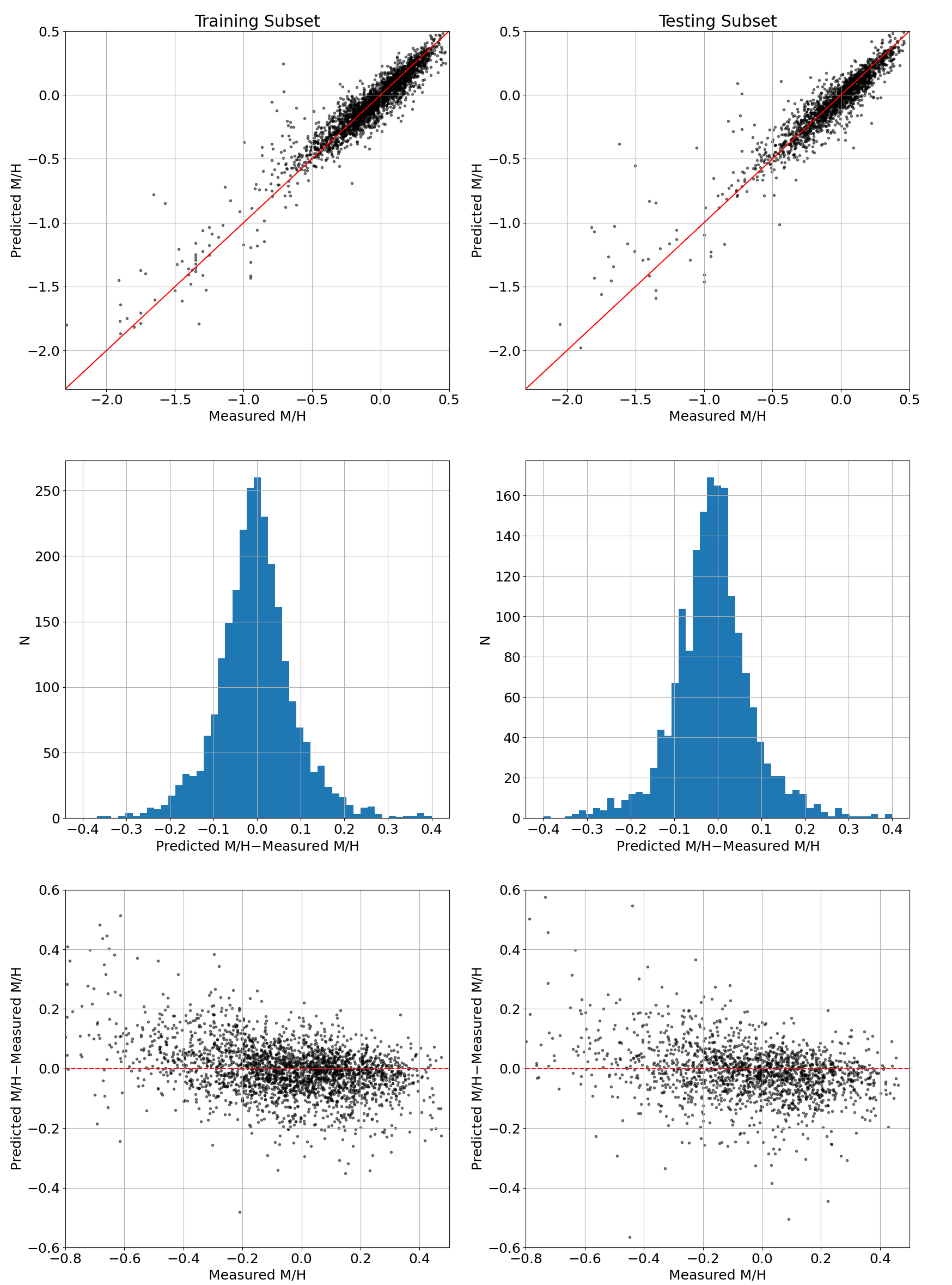
Finally, we use stars in this cleaned sample to perform our final regression. To determine the optimal colors and absolute magnitudes, we use the same iterative method, as discussed above. To reiterate, in this method inputs are iteratively removed, based on the color/absolute magnitude that produces the smallest change in the mean squared error when removed, until only two inputs remain. The optimal colors and absolute magnitudes are then the combination of $N$ inputs that provided the minimum mean squared error for the testing subset during the entire process. For the cleaned sample, the optimal set in this case consists of $M_{g}$, $g-y$, $y-W2$, $J-W2$, $W1-W2$. The results of the regressor for the training subset (the subset used to train the regressor) and the testing subset (the subset used to evaluate the regressor) are shown in Figure 10. A comparison of predicted and observed metallicity (Figure 10, second row) values suggests that the regressor is capable of predicting the metallicities from the input colors and absolute magnitudes to a precision of $\sim$0.12 dex based on the $1\sigma$ scatter. Additionally, the residual error in predicted vs. measured metallicity (Figure 10, bottom row) demonstrates that this scatter is roughly constant over the metallicity range under consideration and that systematic offsets are only apparent at the very metal poor (and sparse) end of the distribution.

Figure 10: Results of the Gaussian Process Regressor on the single-star data set for K and early M dwarfs using the following combination of colors and absolute magnitudes: $M_{g}$, $g-y$, $y-W2$, $J-W2$, $W1-W2$. The first column shows the result for the training subset (the subset used to train the regressor) and the second column the testing subset (the subset used to evaluate the regressor). The top row compares the predicted metallicity from the regressor to the actual value from APOGEE or Hejazi et al. (2020), the middle row shows the distribution of the differences between the predicted and APOGEE metallicity and the bottom rows show the residual error in metallicity versus the measured metallicity.

The actual regressor can be loaded via a Python script; the file with the trained scikit-learn regressor, along with example code to load and use the regressor to predict metallicites, are hosted on our GitHub repository (https://github.com/imedan/gpr_metallicity_relationship).

4.2 M Dwarf Relationship

Next we attempt to determine a photometry-metallicity relationship for M dwarfs cooler than 3500 K, in the same manner as for the K and early M dwarfs (see Section 4.1). The main challenge is to identify a training set for these cooler stars. As discussed above, the stellar parameters for later-type M dwarfs determined from APOGEE are not as reliable as for the K dwarfs. However, since we now have a reliable photometric relationship for the K and early M dwarfs, we can exploit the wide binaries in our high proper motion sample and infer the metallicities of the cooler M dwarf secondaries by proxy of their K dwarf primary. To do this, we use the SUPERWIDE catalog of wide binaries from Hartman & Lépine (2020), which lists $\sim$100,000 high proper motion, wide binaries identified in Gaia through a Bayesian method. Similar to above, the photometry of the stars in each binary is corrected for extinction prior to the analysis. From this catalog, we photometrically select all pairs with a K and early M dwarf primary that also have an M dwarf secondary cooler than 3500 K, again based on the relationship between Gaia photometry and spectral type from Pecaut & Mamajek (2013). Metallicities for the primaries are determined using the final regressor from the Section 4.1 above, and all unresolved binaries for the primary sources are removed using the polynomial relationships and cuts determined for the single star main sequence found in the previous section. This results in a set of 4,859 primary stars, used as proxy for the metallicity values of their cooler M dwarf secondaries. Additionally, we complement this sample with 364 cool, single-star M dwarfs ($<$3500 K) with metallicity estimates from Hejazi et al. (2020).

With this sample of 5,223 cooler M dwarfs now with “observed” metallicity estimates, we train our Gaussian Process Regressor using the same procedure described in Section 4.1 for the K and early M dwarfs. After finding the color and absolute magnitude combination that is the best predictor of metallicity for the M dwarfs, and after removing possible unresolved binaries, our cleaned sample comprises 3,689 stars from the sample of wide binaries and 329 stars from Hejazi et al. (2020). The new polynomial fits to the single star main sequence for the M dwarfs used to clean the sample are shown in Table 10, and Figure 11 shows HR diagrams of the original (left panel) and cleaned (middle panel) samples. Additionally, the right panel of Figure 11 overlays the polynomials from Table 10 on the HR diagram, where it is clear that many of the fits, especially in the metal-poor bins, did not converge on the single-star main sequence. In Section 5.2.2, we will discuss the overall impact of this on the final result.

Table 10: Polynomial fits to the single star main sequence for thirteen bins of metallicity for M dwarfs. Coefficients of the polynomial fits describe the relationship $y=a_{0}+a_{1}x+a_{2}x^{2}+a_{3}x^{3}+a_{4}x^{4}$ where $y=M_{W1}$ and $x=g-W1$. The last two columns of the table give the mean offset and standard deviation, in absolute magnitude, from the relationship; these are used to identify stars deemed over- or under-luminous.

M/H Range	$a_{0}$	$a_{1}$	$a_{2}$	$a_{3}$	$a_{4}$	$\overline{d_{M}}$	$\sigma_{d_{M}}$
$-0.8<M/H\leq-0.7$	-2509	1651	-404.0	43.71	-1.762	-0.1254	0.5188
$-0.7<M/H\leq-0.6$	-4509	3141	-816.7	94.04	-4.046	0.05895	0.5075
$-0.6<M/H\leq-0.5$	-4688	3153	-790.2	87.59	-3.622	0.08001	0.5806
$-0.5<M/H\leq-0.4$	-2098	1427	-362.2	40.76	-1.715	-0.03318	0.3710
$-0.4<M/H\leq-0.3$	2894	-2051	5434.0	-63.86	2.802	-0.03248	0.1901
$-0.3<M/H\leq-0.2$	4704	-3303	867.9	-101.0	4.397	-0.01973	0.3114
$-0.2<M/H\leq-0.1$	-345.4	230.1	-57.08	6.349	-0.2657	-0.02689	0.2953
$-0.1<M/H\leq 0.0$	395.7	-254.7	61.24	-6.422	0.2487	-0.03397	0.2870
$0.0<M/H\leq 0.1$	233.0	-170.5	46.54	-5.521	0.2426	-0.04784	0.3043
$0.1<M/H\leq 0.2$	-349.8	247.6	-65.07	7.620	-0.3334	-0.06066	0.2797
$0.2<M/H\leq 0.3$	770.2	-492.8	117.8	-12.38	0.4845	-0.04733	0.3713
$0.3<M/H\leq 0.4$	665.1	-403.2	91.19	-9.037	0.3320	-0.07541	0.5089
$0.4<M/H\leq 0.5$	-3466	2201	-521.5	54.73	-2.145	0.01033	0.5504

Figure 11: HR diagrams of $M_{W1}$ vs. $g-W1$ for our sample of M dwarf secondaries in common proper motion systems with a K or early M dwarf primary. The left panel is the original subset, the middle panel is the subset after unresolved binaries have been removed, using the method described in Section 4.1, and the right panel shows the polynomial fits from Table 10 overlayed on the subset after the removal of unresolved binaries, where the color of the line corresponds tp the bin of the polynomial fit.

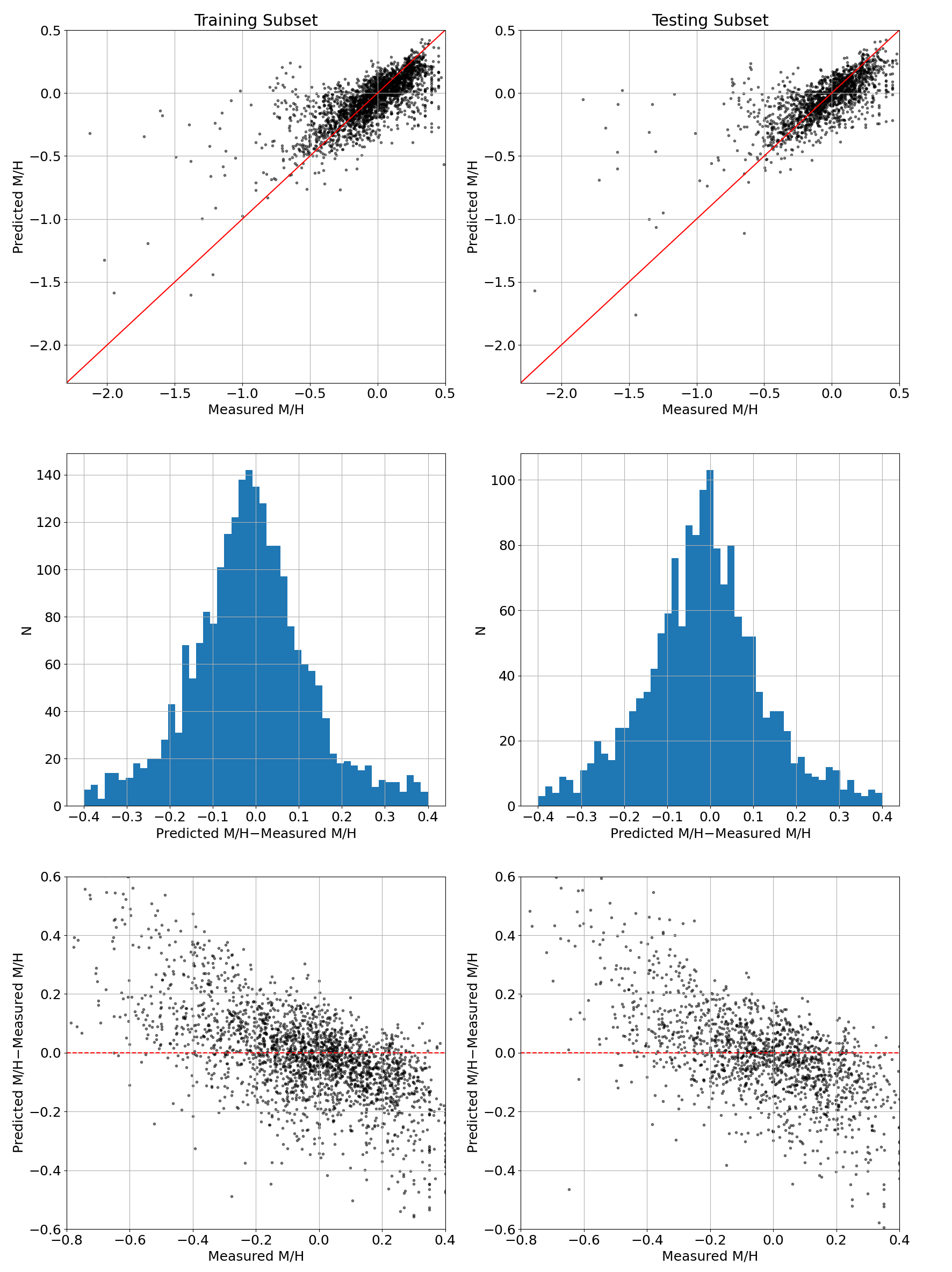
Using this cleaned sample, a final regression is performed to identify the combination of colors and absolute magnitudes that yields the minimal mean squared error for the testing subset. For this subset, the combination of colors and absolute magnitudes that optimizes the final regressor is $M_{r}$, $r-W1$ and $i-K$. The results of the regressor for the training subset (the subset used to train the regressor) and the testing subset (the subset used to evaluate the regressor) are shown in Figure 12. A comparison of the predicted and “observed” metallicity values (Figure 12, top row), suggest that the regressor is generally capable of predicting metallicities from the input colors and absolute with some accuracy. However the regressor struggles with more metal poor stars: the scatter in the predicted vs. “observed” metallicities (Figure 12, middle row) shows a $1\sigma$ spread of 0.21 dex for the testing subset, though this does not account for the compounded error from basing this regressor on the results from the K and early M dwarf regressor. Finally, the residual error in predicted vs. “observed” metallicity (Figure 10, bottom row) demonstrates that this scatter is not uniform over the full metallicity range, and that there are systematic offsets, with metal-poor stars having over-estimated predicted values, and metal-rich stars having under-estimated predicted values.

Figure 12: Results of the Gaussian Process Regressor on the single star data set for M dwarfs using the following combination of colors and absolute magnitudes: $M_{r}$, $r-W1$ and $i-K$. The first column shows the result for the training subset (the subset used to train the regressor) and the second column the testing subset (the subset used to evaluate the regressor). The top row compares the predicted metallicity from the regressor to the “observed” metallicity, i.e., values inferred either from their brighter primaries using our K/early-M regressor or from the spectroscopic analysis of Hejazi et al. (2020), the distribution of the differences between the predicted and APOGEE metallicity, and the bottom row shows the residual error in the predicted versus the “observed” metallicity.

5 Discussion

5.1 Cross-Match Efficiency

The main motivation of this study was to improve the cross-match to external catalogs for Gaia stars with the largest proper motions. Our overall matching rates to the high proper motion subset are listed in Table 11. We compare our percentage of high probability matches to that of the cross-match by Marrese et al. (2019). By extracting our high-proper motion targets with external catalog matches, we found that the Best-Neighbor catalog from Marrese et al. (2019) for the same subset yields the match rates listed in Table 11. The comparison shows that our method, which combines astrometry and photometry, performs better for most catalogs, with the only exception being RAVE DR5.

Table 11: Number of high proper motion sources matched with a total probability $>95\%$

External Catalog	% Matched	% Matched
	[Marrese et al. (2019)]	[This Study]
2MASS	74.8%	75.40%
AllWISE	71.9%	75.17%
GALEX DR5	$\cdots$	8.36%
RAVE DR5	0.92%	0.63%
SDSS DR12	27.9%†	30.69%
Pan-STARRS	14.3%	68.63%

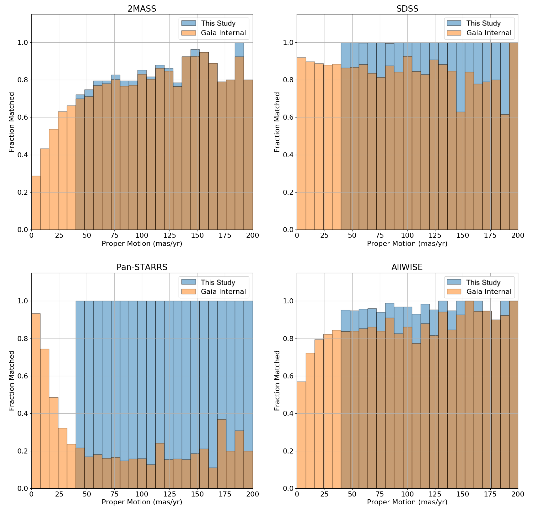
Another way to examine the improvement in the match is to look at the fraction of Gaia sources matched as a function of proper motion for a small, uncrowded region of the sky where all external catalogs should have 100% sky coverage when magnitude limits are not considered. Figure 13 shows this for the four external catalogs with the largest number of matched sources. For external catalogs that are not as deep as Gaia (2MASS and AllWISE), we expect that the fraction matched should decrease with decreasing proper motions, because fainter sources beyond the magnitude limit of the external catalogs are more likely to have small proper motions. This pattern is indeed apparent in the 2MASS and AllWISE recovery rates both from Marrese et al. (2019) and from the present study (see Figure 13). For external catalogs deeper than Gaia (SDSS and Pan-STARRS), we expect that nearly 100% of the Gaia sources should be matched in uncrowded fields. We find this to be the case for our cross-match results, but the Marrese et al. (2019) recovery rates tell a different story, as it is the high proper motion stars that have a lower match rate. In particular, the match to Pan-STARRS from Marrese et al. (2019) is proper motion dependent in a way that suggests significant issues in the Pan-STARRS pipeline in regards to the mean positioning or epoch determination, which then results in poor match rates for high proper motion stars unless these systematic errors are accounted for, as we have done in the present study. We note that these issues also seem present in Marrese et al. (2019) for stars with $\mu<40\ mas\ yr^{-1}$, demonstrating that additional improvements could be made using our method. Performing these matches are outside of the scope of the current study, but volume limited cross-matches are planned for future works.

Figure 13: Recovered fraction of Gaia stars within 3^∘ of $\alpha,\delta=200^{\circ},30^{\circ}$ that were matched to 2MASS, SDSS, Pan-STARRS and AllWISE by this study (blue bins) compared with the recovered fraction in the match by.Marrese et al. (2019) (orange bins). For all external catalogs, this region of sky is 100% covered by the survey, and thus any deviations from a nearly 100% match rate are either due to differences in magnitude limit or some systemic errors in the survey positions.

This large improvement for matching high proper motion stars with Pan-STARRS, when taking into account the footprint of the survey (i.e. $\delta>-30^{\circ}$), results in a match rate of 99.8% for our method, as compared to 20.8% in the same region for the match by Marrese et al. (2019). To demonstrate that our additional matches are genuine, Figure 15 shows the HR diagram using Pan-STARRS photometry combined with matched Gaia parallaxes for three groups: “Same Matches”, consists of Gaia stars that are matched to the same Pan-STARRS source by us and by Marrese et al. (2019); “Different Matches”, consists of Gaia stars that are matched to different Pan-STARRS source by us and by Marrese et al. (2019); and “Mutually Exclusive Matches”, consists of Gaia stars for which one method finds a match while the other does not. This figure shows that the large increase in the match rate is in fact real, as we are getting clean main-sequence, giant, and white dwarf loci for the stars in the mutually exclusive group.

In addition, a look at the “Different Matches” group shows two HR diagrams that look relatively similar in both studies (notably at the faint end), despite matching with different Pan-STARRS sources. We attribute this to the existence of a significant number of duplicates in the Pan-STARRS catalog. This appears to be especially common for high proper motion objects, likely because the Pan-STARRS pipeline is not perfectly able to match detections of fast moving objects at different epochs. The HR diagram from our study, however, does show a “cleaner’” main sequence (with less scatter) at the bright end, which suggests that our study generally finds the Pan-STARRS duplicate entry with the more reliable photometry. Part of this success comes from our more efficient accounting of epoch differences, but also from our Bayesian probability method having a preference for matches with smaller magnitude differences to the Gaia sources, as demonstrated when comparing the 99% lines in the Bayesian probability distributions in Figures 6 and 14.

Figure 14: Probability distributions as discussed in Section 3.4 for Pan-STARRS where $12.5<G\leq 15$ and $19.5\leq|b|<41.8$. Top left panel: frequency distribution for the “true” sample. Top right: frequency distribution for the “displaced sample”. Center left: smoothed frequency distribution for the “true” sample. Center right: modeled frequency distribution for the “displaced” sample. Bottom left: difference between the smoothed “true” frequency distribution and the modeled “displaced” frequency distribution using the correct scaling factor. Bottom right: resulting Bayesian probability distribution. All plots, except for the distribution for $P(H_{1}|\vec{x})$, show the number of sources in a bin on a logarithmic scale and they all share the same colormap range (indicated by the colorbar on the far right). The median and 68th percentile of $i-G$ as a function of $\theta$ are shown on these plots as the red solid and red dashed lines, respectively, where quantiles are found using COBS (Ng & Maechler, 2015). The distribution for $P(H_{1}|\vec{x})$ is shown for a range of 0 to 1 and the overlaid, black solid line shows the 99% line.

Figure 15: HR diagrams combining Pan-STARRS photometry with Gaia parallaxes based on the cross-matches from this study (first column) and the cross-matches from Marrese et al. (2019) (second column). The third column shows the fractional difference between the HR diagrams in the first two columns. The top row shows the “Same Matches”, defined as when both studies find the same match to a Pan-STARRS source (both panels identical by definition); the center row displays the “Different Matches”, defined as when both studies find a match to a Gaia source but determine the best match to be a different Pan-STARRS source; and finally the bottom row shows the “Mutually Exclusive Matches”, defined as when one study finds a match to a Gaia source when the other study finds no suitable match.

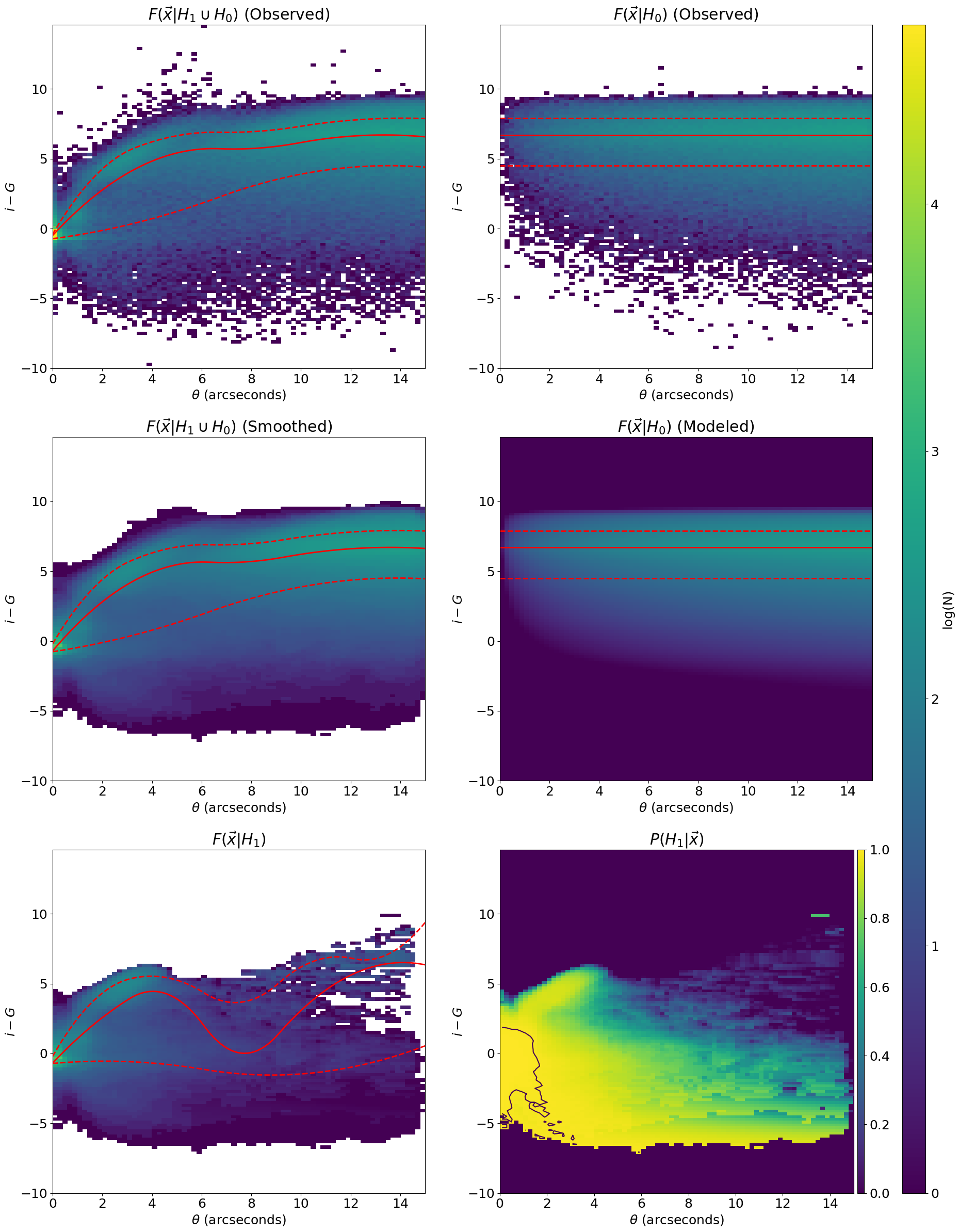
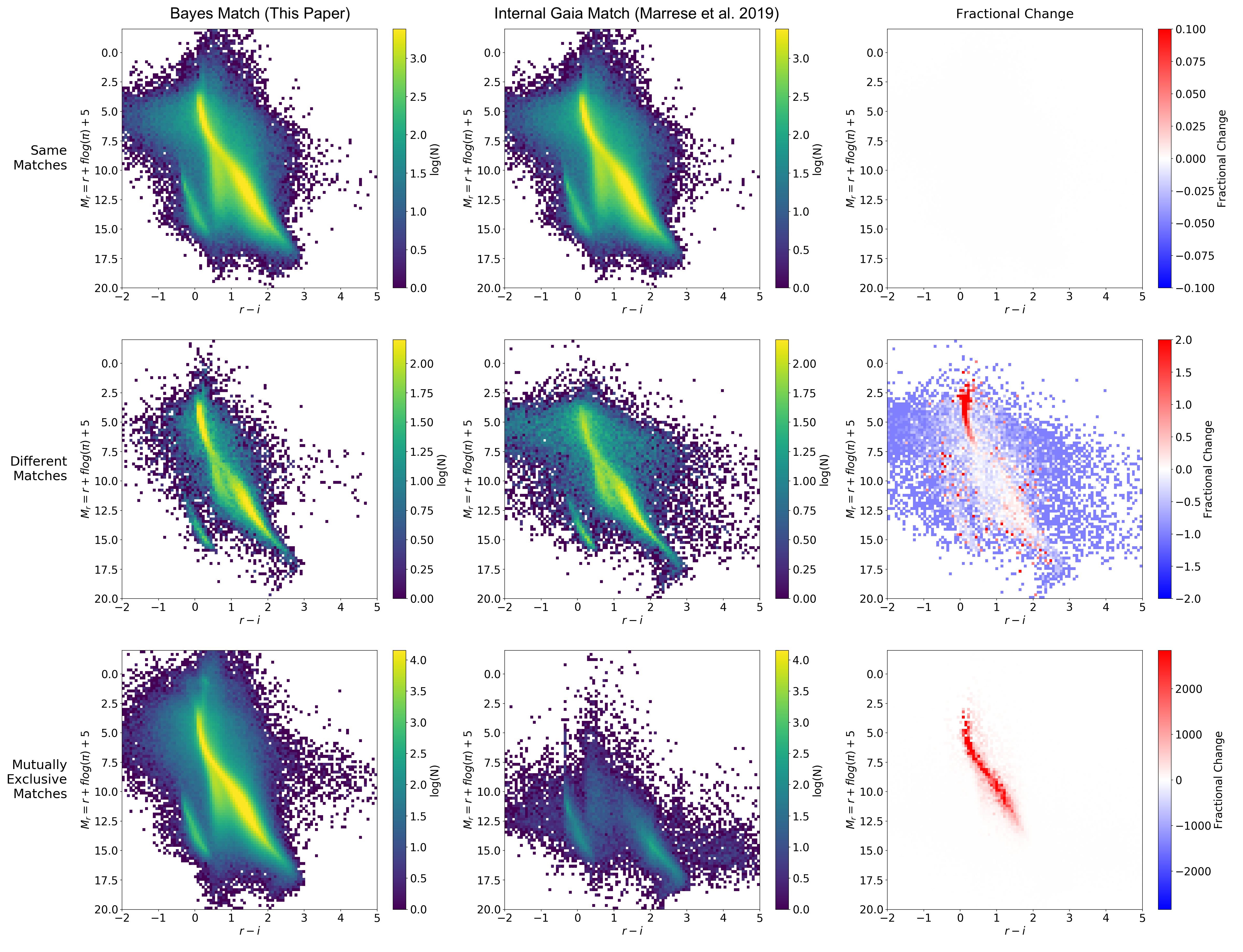
While we see the largest improvement in the Pan-STARSS cross match, we also see modest, but significant, improvements in the cross-match to other catalogs, like SDSS. Figure 16 compares standard $[g-r,r-i]$ color-color diagrams for our match and the match by Marrese et al. (2019), where the layout is the same as in Figure 15. Two notable trends are apparent. First, we do find that for some matches that differ between the studies (“Different Matches” group) our cross-match again produces a cleaner subset with better photometry, i.e., more consistent with the expected main-sequence locus, which suggest that our match is more accurate. Second, we can see in the “Mutually Exclusive Matches” group that our matches shows a denser main-sequence locus, and also show a clear “white dwarf-M dwarf binary bridge”, which is a well-known arc that connects the white dwarf and M dwarf loci on the color-color diagrams (e.g. Augusteijn et al., 2008; Liu et al., 2012). In contrast, the “Mutually Exclusive Matches” from Marrese et al. (2019), show more stars with poor or inconsistent photometry, notably stars in a diagonal locus redder in $r-i$ than the expected M dwarf locus, and with inconsistent colors for a nearby main-sequence star.

Figure 16: Standard $[g-r,r-i]$ color-color diagram of the SDSS DR12 sources matched in this study (first column) and of the SDSS DR9 match done by Marrese et al. (2019) (second column). The third column shows the fractional difference between the color-color diagrams in the first two columns, where all color maps are centered on zero, which is represented as white in the color map. Three subsets are represented: “Same Matches”, defined as when both matches find the same match to a Pan-STARRS source (top row; identical for both studies by definition); “Different Matches”, defined as when both matches find a match to a Gaia source but we determine the best match to be a different Pan-STARRS source (center row); and “Mutually Exclusive Matches”, defined as when one match found a match to a Gaia source when the other match did not (bottom row).

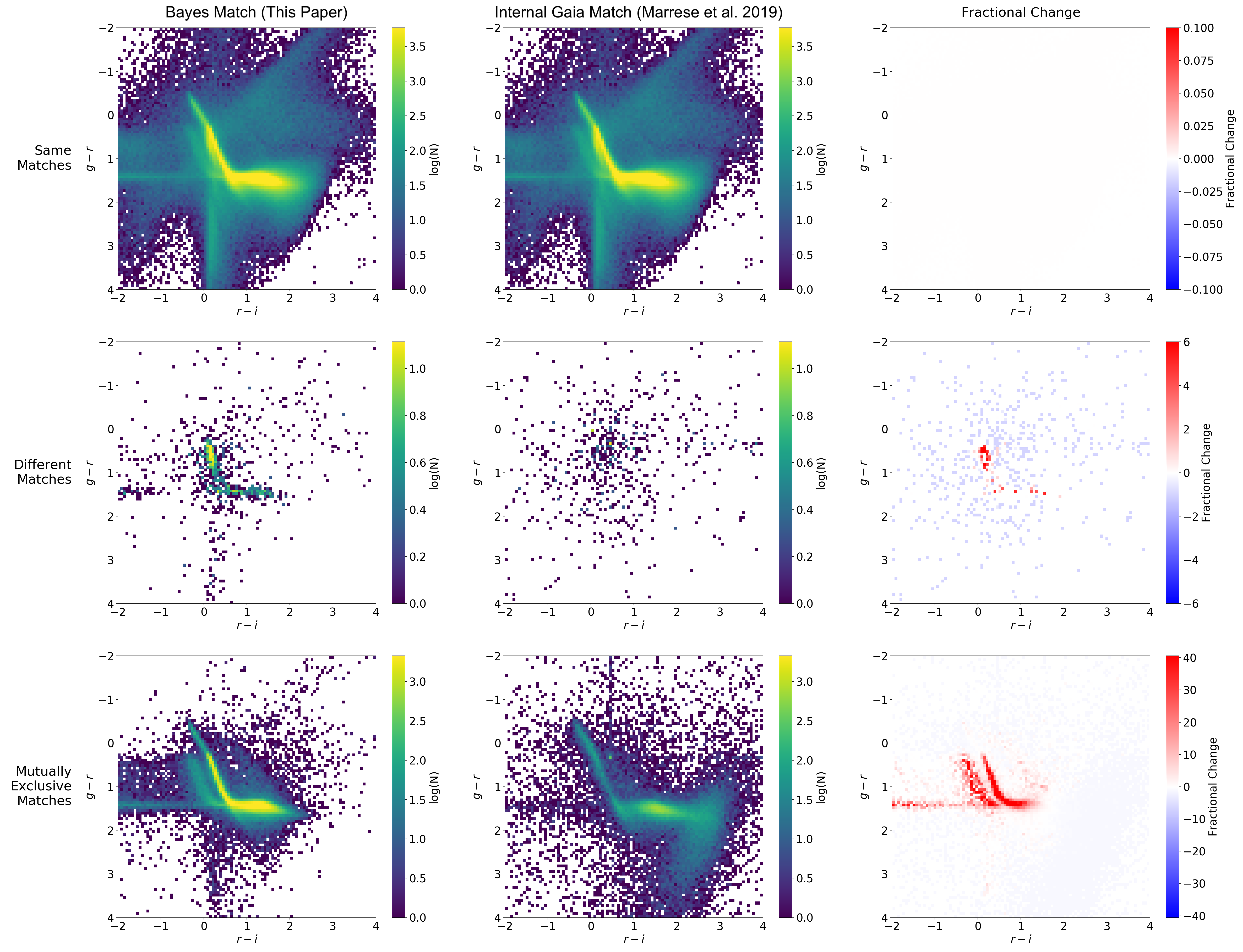
Overall, this demonstrates that our cross-match method not only produces a more complete catalog of counterparts, but also provides cleaner photometry. Our catalog of cross-matches is also “probabilistic”, and users can lower the probability threshold in order to get a more complete catalog at the expense of having a higher rate of false matches.

5.2 Photometric Metallicity Relationships

5.2.1 K and Early M Dwarf Relationship

Using machine learning with a Gaussian Process Regressor, we show that it is possible to predict the metallicity of stars in a testing subset of K and early M dwarfs to within $\pm$0.12 dex, using a combination of absolute magnitudes and color terms. For comparison, past efforts to determine photometric metallicities in the same temperature range by Schmidt et al. (2016) and Davenport & Dorn-Wallenstein (2019) could predict metallicities with a claimed precision of 0.18 dex and 0.11 dex, respectively. However both studies used relatively metal-rich subsets, with the relationship from Schmidt et al. (2016) tested over $-1<M/H<0.2$ and Davenport & Dorn-Wallenstein (2019) over $-1<M/H<0.5$. The relationship from Schmidt et al. (2016) also covered a smaller temperature range of $3550<T_{eff}<4200$, while the temperature range for Davenport & Dorn-Wallenstein (2019) is unclear. In contrast, our regressor is calibrated over a broader range of metallicities ($-2.3<M/H<0.5$) and temperatures ($3500<T_{eff}<5280$ K).

Compared with the relationship of Schmidt et al. (2016), we find that our calibration, besides improving on precision, also significantly improves on known systematic errors. Figure 5 from Schmidt et al. (2016), shows that predicted metallicity values for metal-poor stars are systematically over-estimated, while predicted values for metal-rich stars are systematically under-estimated. Such a trend is not observed with our regressor (Figure 10, bottom row). These systematic errors are likely due to contamination from unresolved binaries in their sample, which is exactly what we have attempted to correct for in the present study. To demonstrate this effect, Figure 17 shows the results from our regressor when it is trained and evaluated on the K and early M dwarf data set before the unresolved binaries are removed. Not only is the scatter greater when the binaries are left in (Figure 17, first and second row), but the residuals between the photometric metallicity estimates and the measured metallicity values show the same systematic errors as in previous studies (Figure 17, third row). This demonstrates the importance of removing such contaminates from the training sample before extracting a relationship between photometry and metallicity. Another important distinction between our study and Schmidt et al. (2016) is that our regressor uses Pan-STARRS for the optical magnitudes, while Schmidt et al. (2016) uses those from SDSS. Due to the much larger sky coverage of Pan-STARRS (including large swaths of the Galactic plane overlooked by SDSS), our regressor can be used for a much larger number of stars than that of Schmidt et al. (2016).

Figure 17: Results of the Gaussian Process Regressor on the training set of K and early M dwarfs but with no preliminary removal of suspected binaries (compare with Figure 10), and again using the following combination of colors and absolute magnitudes: $M_{g}$, $g-y$, $y-W2$, $J-W2$, $W1-W2$. The first column shows the result for the training subset (the subset used to train the regressor) and the second column the testing subset (the subset used to evaluate the regressor). The top row compares the predicted metallicity from the regressor to the actual value from APOGEE, the middle row shows the distribution of the differences between the predicted and APOGEE metallicity, and the bottom row shows the residual error in metallicity versus the APOGEE metallicity. Compared with the training subset cleaned of suspected binaries (Figure 10), this “unclean” subset yields a regressor which introduces significantly larger systematic and random errors, thus demonstrating the need to use a “cleaned” training subset.

Davenport & Dorn-Wallenstein (2019) also used a machine learning technique, with a k-nearest neighbors regressor, in order to estimate photometric metallicities. They have provided their code and data set used for training, and we have used these to predict metallicites for their training sample. We have also included $M_{G}$ as part of the inputs for their regressor, which they note improves the final results. The results from the Davenport & Dorn-Wallenstein (2019) regressor are shown in Figure 18 for comparison. The scatter in the distribution is found to be comparable to that from our own regressor, although the tails of our scatter distribution are much lower, the systematic trend of the metallicities of metal-poor stars being over-estimated, and the metallicities of metal-rich stars being underestimated is however stronger in the Davenport & Dorn-Wallenstein (2019) regressor results, suggesting that the sample used for training includes contaminates in the form of unresolved binaries which are skewing the results.

Figure 18: Results of the k-nearest neighbors regressor from Davenport & Dorn-Wallenstein (2019). The left panel compares the predicted metallicity from the regressor to the actual value from APOGEE, the middle panel shows the distribution of the differences between the predicted and APOGEE metallicity for Davenport & Dorn-Wallenstein (2019) (blue bins) and this study (orange bins), and the right panel shows the residual error in metallicity versus the APOGEE metallicity.

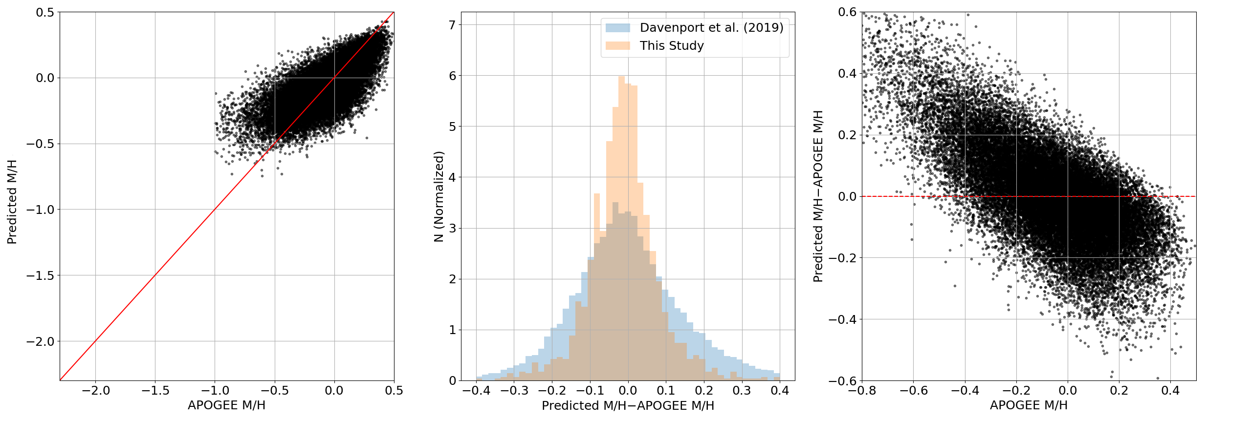
5.2.2 M Dwarf Relationship

While our removal of unresolved binaries in the K and early M subset appears to be successful in reducing systematic errors, we cannot currently achieve the same results for our M dwarf calibration. Our current M dwarf regressor does show significant systematic errors consistent with binary star contamination (Figure 17), which suggests that our attempted removal of unresolved binaries is less effective than in the K and early M subset. This result is affirmed by the polynomial fits in the right panel of Figure 11, where it is clear the fits did not converge and effectively remove all of the unresolved binaries. This result is to be expected if we consider that the width of the main sequence is significantly wider for M dwarfs, thus making the removal of unresolved binaries more challenging with our polynomial method. Binary removal is especially challenging for metal-poor stars, which have minimal representation in the training subset in any case.

To further illustrate the challenge of training a regressor for metal-poor M dwarfs, we applied both of the trained regressors to the entirety of the cross matched high proper motion sample in this study. This resulted in 716,651 K and early M dwarfs, and 1,030,761 M dwarfs that have the required photometry, have a parallax error $<20\%$, have passed the single star polynomial fit pass, and have predicted metallicities within the range of the training subsets (i.e. $-2.3<M/H<0.5$). The estimated metallicity values are listed in Tables 12 and 13. Elimination of suspected binaries using our polynomial cut method removed 23% of the K dwarfs and 10% of the M dwarfs. HR diagrams of these samples are presented in Figure 19, and show a clear deficit of stars at the metal-poor (blue) edge of the main-sequence locus. Figure 20 shows that the distribution of metal-poor K and early-M stars is very spread out compared with the distribution of metal-rich objects, which is more local. The difference comes from the metal-poor stars coming from the local thick disk and halo population, which has a much lower density near the Sun. Figure 21 shows that this is a problem for locating metal-poor M dwarfs, because the Gaia catalog identifies them to a significantly shorter distance range, biasing the sample in favor of more metal-rich M dwarfs

Table 12: List of predicted metallicities for 716,651 K and early M dwarfs using the Gaussian Process Regressor outlined in Section 4.1. The regressor uses the following data inputs, $M_{g}$, $g-y$, $y-W2$, $J-W2$, $W1-W2$, and stars are included only if they pass the single star polynomial cuts outline in Table 9.

Gaia ID	$\alpha_{Gaia}$	$\delta_{Gaia}$	M/H	$\sigma_{M/H}$
	[deg]	[deg]	[dex]	[dex]
2738617902668633344	0.00059265319	1.41569388809	0.182	0.055
2420684907087327104	0.00064439500	-14.44069806218	0.175	0.057
384458916557103744	0.00098644795	42.92964411582	-0.100	0.063
2422936569461883648	0.00149210844	-9.59710946245	-0.320	0.057
2422910181182822784	0.00181091004	-9.91118104462	0.138	0.054
2448241275523065856	0.00190792593	-2.76638530879	-1.609	0.156
2335002057582474752	0.00194199280	-25.60630079213	0.302	0.056
2334659529646655744	0.00206867958	-26.54384648213	-0.268	0.065
2341416475275983872	0.00212583048	-21.25877753606	0.424	0.057
2414490258576137984	0.00254114360	-17.08225464560	-0.129	0.063

Note. — This table is published in its entirety in the machine-readable format. A portion is shown here for guidance regarding its form and content.

Table 13: List of predicted metallicities for 1,030,761 M dwarfs using the Gaussian Process Regressor outlined in Section 4.2. The regressor uses the following data inputs, $M_{r}$, $r-W1$ and $i-K$, and stars are included only if they pass the single star polynomial cuts outline in Table 10.

Gaia ID	$\alpha_{Gaia}$	$\delta_{Gaia}$	M/H	$\sigma_{M/H}$
	[deg]	[deg]	[dex]	[dex]
429379051804727296	0.00021864741	60.89771179398	0.051	0.133
384318827606840448	0.00047931984	42.19465632646	0.308	0.140
2772104109112208256	0.00051294158	15.56517501763	0.039	0.133
2846731811580119040	0.00115069265	21.30261306611	0.329	0.148
2441058204714858240	0.00121147731	-8.90793754062	-0.230	0.138
386559121204819328	0.00193074605	45.04225289803	0.173	0.156
2313055461894623232	0.00204668844	-33.55516167237	-0.008	0.181
2421214317639640064	0.00231957574	-12.53175806608	-0.155	0.133
2334666126716440064	0.00256127213	-26.36534090966	-0.071	0.133
2443194001755562624	0.00271533083	-5.07308824110	0.281	0.138

Note. — This table is published in its entirety in the machine-readable format. A portion is shown here for guidance regarding its form and content.

Figure 19: HR diagrams for the 716,651 K and early M dwarfs (top row), and for the 1,030,761 M dwarfs (bottom) for which we estimated metallicities using our Gaussian Process regressor, with the metallicity values shown as a color scale in the panels on the left, and the accuracy of the estimate shown as a color scale in the panels on the right. These represent all stars with the required photometry in the cross matched high proper motion sample, that have a parallax error $<20\%$, have passed the single star polynomial fit pass, and have predicted metallicities within the range of the training subsets (i.e. $-2.3<M/H<0.5$) shown on respective HR diagrams. The panels on the right show the 95% confidence interval for the metallicity measurements shown in the left column.

Figure 20: Height above the Galactic plane (z) versus Galactocentric radius for the 716,651 K and early M dwarfs with metallicity values estimated from our Gaussian Process Regressor (see Figure 19). Each panel shows a subset in a defined metallicity range, with more metal poor stars near the top and more metal rich stars near the bottom. Metal-poor stars show a more dispersed distribution consistent with old disk and halo membership, which metal-rich stars show a more pronounced concentration near the Galactic midplane.

Figure 21: Height above the Galactic plane (z) versus Galactocentric radius for the 1,030,761 M with metallicity values estimated from our Gaussian Process Regressor (see Figure 19). Each panel shows a subset in a defined metallicity range, with more metal poor stars near the top and more metal rich stars near the bottom. Compared with the K and early M dwarf distribution shown in Figure 20, the M dwarf distribution appears significantly more distance limited, which is due to the Gaia magnitude limit. This prevents the inclusion of larger numbers of metal-poor objects.

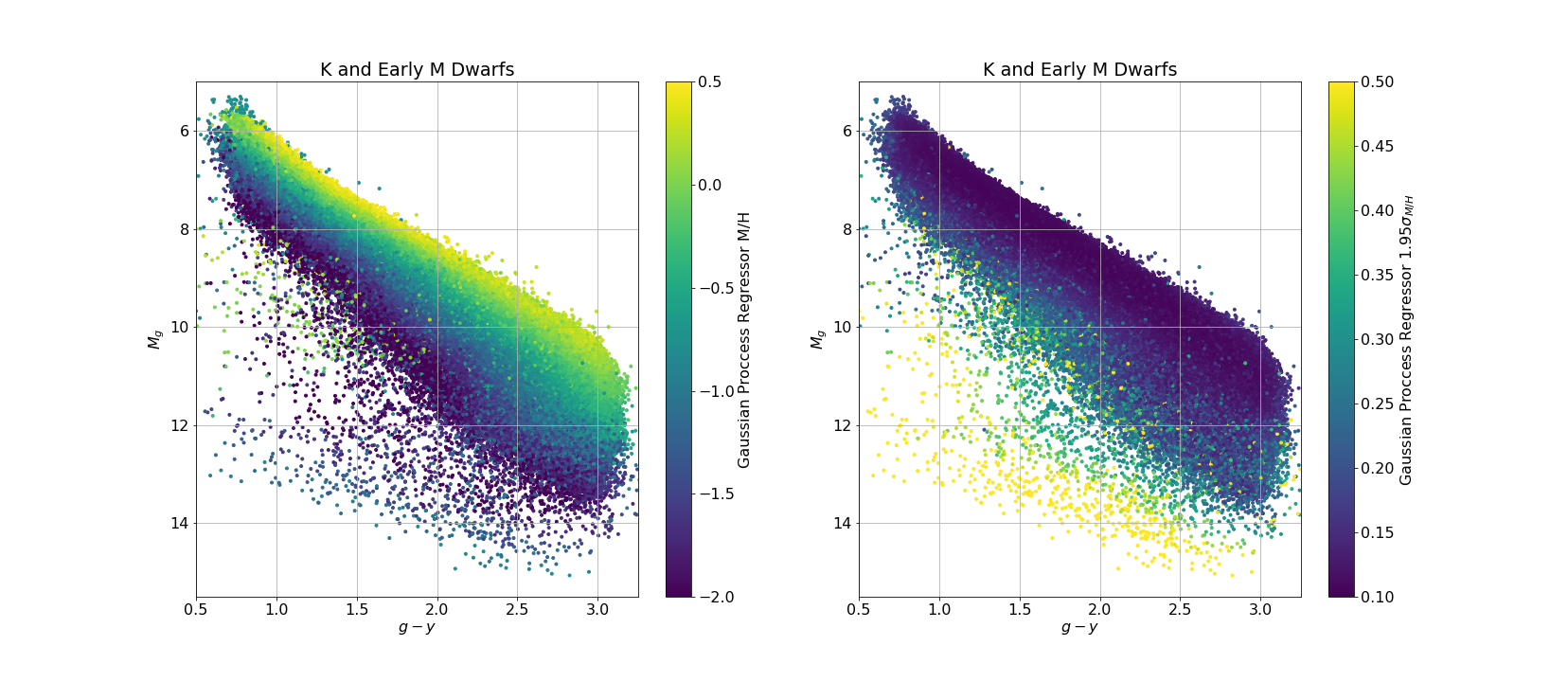
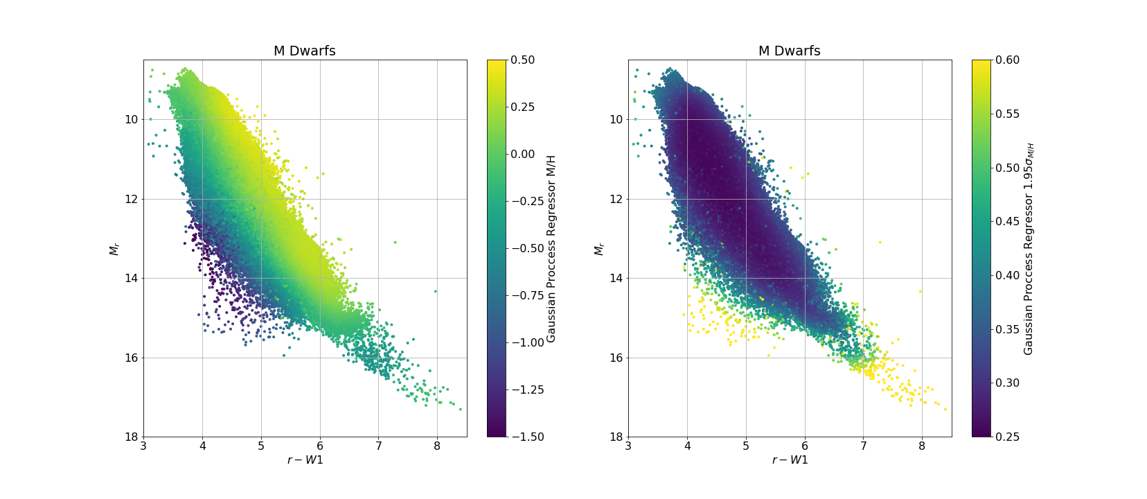
In the Gaussian Processor Regression method, standard deviations of predicted values can be computed, and these are represented as the color scale in the right panels of Figure 19. We find that for the highly sampled metallicity regime (i.e. $-0.6<M/H<0.5$ for both samples) the 95% confidence of our sample is comparable to the $1\sigma$ spread we found in the testing subset for each regressor. However, the errors become much larger for lower metallicity regimes and regions of the HR diagram that are not as well sampled in the training subset. This is a good indicator that while there are limitations with both of these regressors, the predicted errors at least allow us to determine the range over which the method yields the best results.

Knowing that stellar kinematics is locally correlated with chemical abundances, we validate our predicted metallicity values by examining the range of metallicity estimates for various subsets of K and M dwarfs selected by tangential velocity (Figure 22). For the K and early M dwarfs (Figure 22, left panels), we observe the trend noted in previous studies (e.g. Nordström et al., 2004; Ivezić et al., 2008; Bensby et al., 2014; Grieves et al., 2018) showing a steep negative metallicity gradient as a function of tangential velocity. The trend is however not observed for our subset of M dwarfs (Figure 22, right panels) which shows few metal-poor stars, even at large tangential velocities. We suggest that this again is due to the inherent bias in the initial magnitude-limited, high proper motion Gaia subset, which is efficient at selecting more distant, high velocity K dwarfs of the thick disk and halo, but does a poor job at identifying their M dwarf equivalents because of magnitude limit. In order to improve our metallicity calibration for the M dwarfs, we would need to include a larger sample of nearby, metal-poor M dwarfs in our training subset, which likely will depend on the use of deeper surveys like SDSS, Pan-STARRS, and the upcoming LSST (Ivezić et al., 2019).

Figure 22: Distribution of estimated photometric metallicity values for different cuts of tangential velocity (top row) and photometric metallicity as a function of tangential velocity (bottom row) for the 716,651 K and early M dwarfs (bottom left column) and 1,030,761 M dwarfs (bottom right panel). The red data points and error bars represent the average and standard deviation, respectively, of the predicted metallicity in bins of 50 km/s of tangential velocity. The apparent lack of metal-poor M dwarfs is due to selection effects from the magnitude limit of of the Gaia catalog.

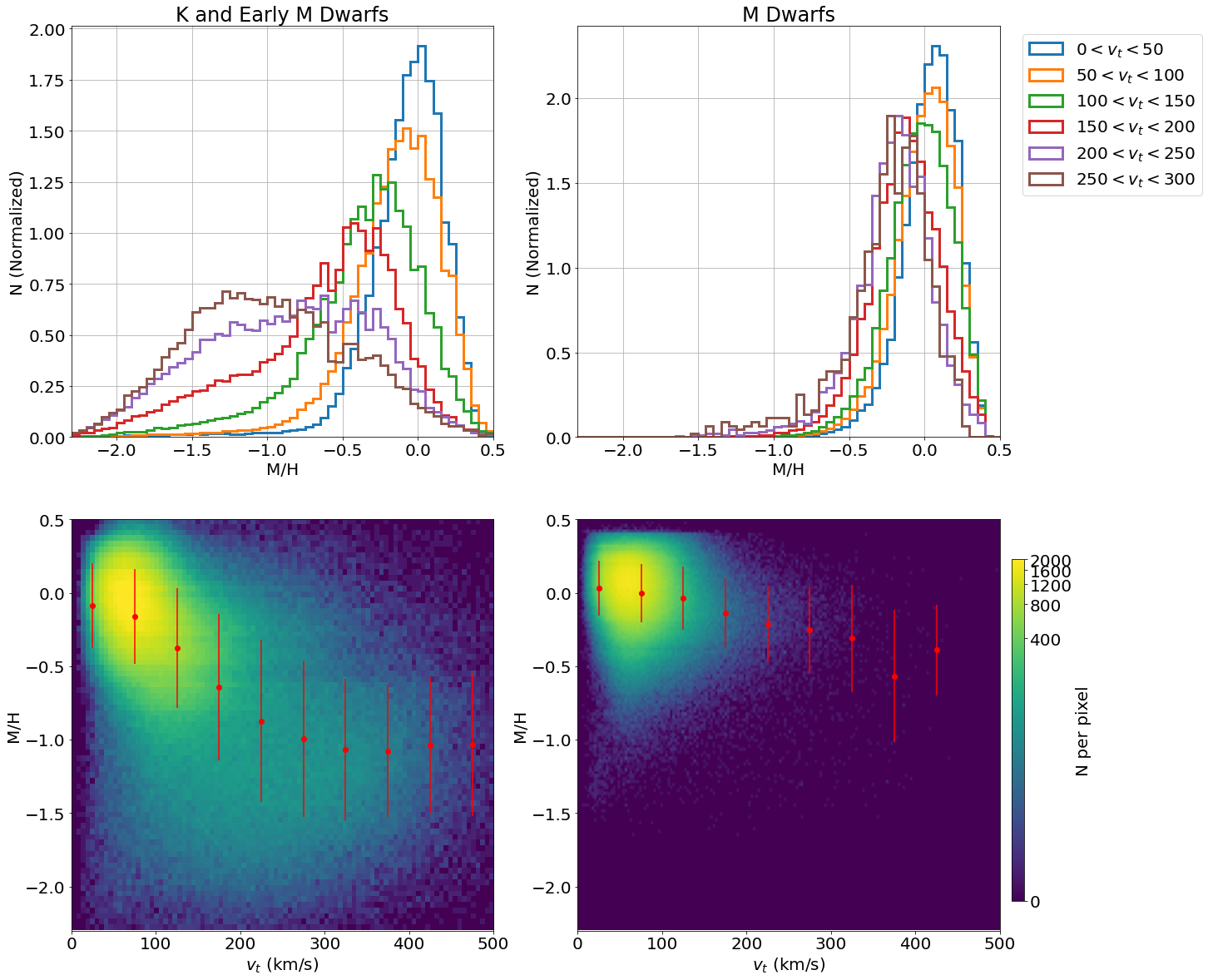
5.2.3 Photometric Metallicities of Nearby Clusters: Hyades and Praesepe

As a final check on our calibrations, we verify the average metallicity of stars in our high proper motion sample (from Section 5.2.2) that are members of nearby open clusters. Specifically, we consider stars that are members of the Hyades and Praesepe open clusters. We use the open cluster members from Gaia Collaboration et al. (2018a), where members were chosen using an iterative process that determines the cluster velocity and location centroid, as detailed in Gaia Collaboration et al. (2017). We use the Gaia IDs from Gaia Collaboration et al. (2018a) to identify members in our high proper motion sample. The distributions of photometric metallicities from both calibrations are shown in Figure 23. The number of cluster members displayed in Figure 23 is lower than the count from Gaia Collaboration et al. (2018a), especially for the K and early M dwarfs, because we only estimate metallicities for stars with $g_{PS1}<13.5$ mag to avoid saturation errors.

Figure 23: Distributions of estimated photometric metallicities for the subset of K and early M dwarfs (top row), and for the subset of later-type M dwarfs (bottom row) for members of the Hyades (left column) and Praesepe (right column), where membership of these open clusters is from Gaia Collaboration et al. (2018a). The solid black line is a fitted Gaussian distribution to the histogram. Gaussian fits are shown with the black line, and the measured mean and dispersion values are noted with the black dots and their errobars. For the K and early M dwarf members of the Hyades, the one member at $[M/H]\approx-0.2$ dex (light blue histogram) has not been included in the mean for the cluster as it presented as a clear outlier on an HR diagram. The cluster averages are compared to the spectroscopically derived cluster metallicity estimates from Netopil et al. (2016) (red data points and errorbars); our average and RMS errors for the Hyades are $\overline{M/H}_{RMS}=0.120\pm 0.039$ for the K and early M Dwarfs, and $\overline{M/H}_{RMS}=0.200\pm 0.068$ for the M dwarfs, as compared to $\overline{M/H}_{RMS}=0.13\pm 0.05$ from Netopil et al. (2016). The average and RMS errors for Praesepe are $\overline{M/H}_{RMS}=0.130\pm 0.064$ for the K and early M Dwarfs, and $\overline{M/H}_{RMS}=0.185\pm 0.073$ for the M dwarfs, as compared to $\overline{M/H}_{RMS}=0.16\pm 0.08$ from Netopil et al. (2016).

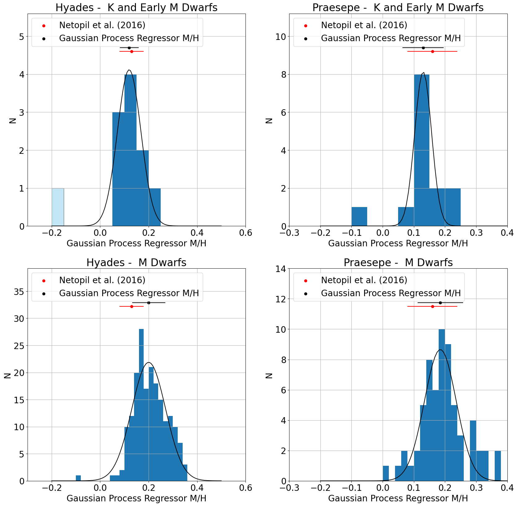
A Gaussian fit to the K/early-M metallicity distribution of Hyades members shows an average value of $\overline{M/H}=0.120$ and a dispersion of $\sigma_{M/H}=0.048$. For the M dwarfs, we find $\overline{M/H}=0.200$ and a dispersion of $\sigma_{M/H}=0.070$. A Gaussian fit to the K/early-M dwarf in Praesepe yields a average value $\overline{M/H}=0.130$ with a dispersion $\sigma_{M/H}=0.027$, while the M dwarf distribution yields $\overline{M/H}=0.185$ with a dispersion $\sigma_{M/H}=0.051$. We compare these values to the metallicity estimates from Netopil et al. (2016), which provides metallicities derived from open cluster members with high quality spectra. To be consistent with their results, we present our averages, from the fitted Gaussian distributions, along with the RMS error, which are shown as the data points in Figure 23. Additionally, for the K and early M dwarf members of the Hyades, the one member at $[M/H]\approx-0.2$ dex (light blue histogram in Figure 23) has not been included in the mean for the cluster as it presented as a clear outlier on an HR diagram of the cluster members presented here. The average and RMS errors for the Hyades are $\overline{M/H}_{RMS}=0.121\pm 0.406$ for the K and early M Dwarfs, and $\overline{M/H}_{RMS}=0.200\pm 0.068$ for the M dwarfs, as compared to $\overline{M/H}_{RMS}=0.13\pm 0.05$ from Netopil et al. (2016). The average and RMS errors for Praesepe are $\overline{M/H}_{RMS}=0.130\pm 0.064$ for the K and early M Dwarfs, and $\overline{M/H}_{RMS}=0.185\pm 0.073$ for the M dwarfs, as compared to $\overline{M/H}_{RMS}=0.16\pm 0.08$ from Netopil et al. (2016). It seems that, within the uncertainties, our photometric calibrations agree with the spectroscopic estimates from Netopil et al. (2016).

From this test alone, we cannot however rule out systematic errors in our calibrations. This is because the metallicity probed by these two clusters is in a region in metallicity where the results from our calibration indicate either no systematic errors (K and early M dwarfs, Figure 10) or considerably lessened systematic errors (M Dwarfs, Figure 12), as compared to more metal-poor and metal-rich regimes. A test of the metal-poor and metal-rich regimes may prove difficult due to the limited number of nearby stars clusters, and may have to rely on more direct spectroscopic metallicity measurements from individual stars. With this in mind, we remain cautious about the application of our regressors for metal-poor systems, but with the results in this section do feel confident about the metallicity estimates provided for M dwarfs in the local disk population of the Milky Way.

6 Conclusions

In this study we sought to develop a Bayesian framework for cross-matching high proper motion stars in Gaia to photometric external catalogs of various size and wavelength coverage. This was accomplished by comparing two dimensional distributions that take into account photometry and astrometry of a “true” initial catalog query and a “displaced” catalog query, used to infer the distribution of random field stars. Using these distributions, we are able to find match probabilities for all stars within 15” of our Gaia sources at the mean epoch of the external survey. These sources and their Bayesian match probabilities are included in an accompanying electronic table.

When comparing the counterparts with the highest match probabilities ($>$95%) to the counterparts found in the internal Gaia cross-match presented in Marrese et al. (2019), we find that our method produces a better match rate, with the largest improvement achieved for Pan-STARRS. Additionally, we show that the photometry produced by our method creates a “cleaner” catalog overall, with fewer stars having clearly incorrect colors due to mismatches.

With this more complete cross matched catalog of high proper motion sources, we identify a training subset of 4,378 K and early M dwarfs with metallicity values measured from SDSS-APOGEE spectra, and recover their optical and infrared photometry from Pan-STARRS, 2MASS, and AllWISE. We use this training subset to derive a Gaussian Process Regressor that yields metallicity estimates based on the optical and infrared photometry. Our regressor applies to K and early M dwarfs in the color range $0.98<BP-RP<2.39$ mag. In addition, we apply the results of the first regressor on a set of 3,689 common proper motion binaries and infer metallicity for the later-type M dwarf companions in these systems. We use this as a training subset to create a second Gaussian Process Regressor, which we use to estimate metallicities in later type M dwarfs, in the color range $2.39<BP-RP<5$ mag.

We found that our K and early M dwarf regressor performs better than previously calibrated photometric metallicity relationships, with noticeably smaller random and systematic errors, and an effective range extending to significantly more metal-poor populations than in previous work. For the M dwarf regressor, we find larger random errors for the testing subset along with systematic offsets, which we attribute to the contaminating presence of unresolved binaries in our training subset.

When applying these regressors to the full catalog of high proper motion stars, we find that the metallicity estimates are consistent with that we would expect from the stellar populations probed by our sample based on their location (galactic height) and kinematics (old/young population). Additionally, when we examine the metallicity distributions of stars in our sample that are members of the Hyades and Praesepe open clusters, we find average metallicity values that are consistent with values measured with high resolution spectroscopy of the more massive cluster members. While we do not notice any systematic errors for these clusters, we are not yet able to test the relationship for the more critical metal-poor metallicity regime, due to limitations with the high proper motion/low-mass sample which restricts the census to very local populations. The validation of the relationship in the metal-poor regime might require direct metallicity measurements through spectroscopic observations. Additionally, for the M dwarf regressor specifically, we note that systematic errors are still present to some degree throughout the metallicity range probed, which is indicative of unresolved binaries in our training sample. Future work will need to be done in order to better remove unresolved binaries from the training subset in order to improve the regression and mitigate these issues.

References

- Alam et al. (2015) Alam, S., Albareti, F. D., Allende Prieto, C., et al. 2015, ApJS, 219, 12
- Allard et al. (1997) Allard, F., Hauschildt, P. H., Alexander, D. R., & Starrfield, S. 1997, ARA&A, 35, 137
- Augusteijn et al. (2008) Augusteijn, T., Greimel, R., van den Besselaar, E. J. M., Groot, P. J., & Morales-Rueda, L. 2008, A&A, 486, 843
- Bensby et al. (2014) Bensby, T., Feltzing, S., & Oey, M. 2014, aap, 562, A71
- Bianchi et al. (2011) Bianchi, L., Herald, J., Efremova, B., et al. 2011, Ap&SS, 335, 161
- Bochanski et al. (2010) Bochanski, J. J., Hawley, S. L., Covey, K. R., et al. 2010, AJ, 139, 2679
- Bonfils et al. (2005) Bonfils, X., Delfosse, X., Udry, S., et al. 2005, A&A, 442, 635
- Budavári & Szalay (2008) Budavári, T., & Szalay, A. S. 2008, ApJ, 679, 301
- Buitinck et al. (2013) Buitinck, L., Louppe, G., Blondel, M., et al. 2013, in ECML PKDD Workshop: Languages for Data Mining and Machine Learning, 108–122
- Casagrande et al. (2008) Casagrande, L., Flynn, C., & Bessell, M. 2008, MNRAS, 389, 585
- Casagrande et al. (2010) Casagrande, L., Ramírez, I., Meléndez, J., Bessell, M., & Asplund, M. 2010, A&A, 512, A54
- Chambers et al. (2016) Chambers, K. C., Magnier, E. A., Metcalfe, N., et al. 2016, arXiv e-prints, arXiv:1612.05560
- Cutri & et al. (2014) Cutri, R. M., & et al. 2014, VizieR Online Data Catalog, II/328
- Davenport & Dorn-Wallenstein (2019) Davenport, J. R., & Dorn-Wallenstein, T. Z. 2019, Research Notes of the American Astronomical Society, 3, 54
- Davenport et al. (2014) Davenport, J. R., Ivezić, Ž., Becker, A. C., et al. 2014, mnras, 440, 3430
- Dittmann et al. (2016) Dittmann, J. A., Irwin, J. M., Charbonneau, D., & Newton, E. R. 2016, ApJ, 818, 153
- Eisenstein et al. (2011) Eisenstein, D. J., Weinberg, D. H., Agol, E., et al. 2011, AJ, 142, 72
- Gaia Collaboration et al. (2017) Gaia Collaboration, van Leeuwen, F., Vallenari, A., et al. 2017, A&A, 601, A19
- Gaia Collaboration et al. (2018a) Gaia Collaboration, Babusiaux, C., van Leeuwen, F., et al. 2018a, aap, 616, A10
- Gaia Collaboration et al. (2018b) Gaia Collaboration, Brown, A. G. A., Vallenari, A., et al. 2018b, A&A, 616, A1
- Ginsburg et al. (2019) Ginsburg, A., Sipőcz, B. M., Brasseur, C. E., et al. 2019, AJ, 157, 98
- González Hernández & Bonifacio (2009) González Hernández, J. I., & Bonifacio, P. 2009, A&A, 497, 497
- Green et al. (2019) Green, G. M., Schlafly, E., Zucker, C., Speagle, J. S., & Finkbeiner, D. 2019, apj, 887, 93
- Grieves et al. (2018) Grieves, N., Ge, J., Thomas, N., et al. 2018, mnras, 481, 3244
- Hartman & Lépine (2020) Hartman, Z. D., & Lépine, S. 2020, ApJS, 247, 66
- Hejazi et al. (2020) Hejazi, N., Lépine, S., Homeier, D., Rich, R. M., & Shara, M. M. 2020, AJ, 159, 30
- Holtzman et al. (2018) Holtzman, J. A., Hasselquist, S., Shetrone, M., et al. 2018, The Astronomical Journal, 156, 125
- Ivezić et al. (2008) Ivezić, Ž., Sesar, B., Jurić, M., et al. 2008, apj, 684, 287
- Ivezić et al. (2019) Ivezić, Ž., Kahn, S. M., Tyson, J. A., et al. 2019, ApJ, 873, 111
- Kunder et al. (2017) Kunder, A., Kordopatis, G., Steinmetz, M., et al. 2017, AJ, 153, 75
- Lépine & Bongiorno (2007) Lépine, S., & Bongiorno, B. 2007, AJ, 133, 889
- Lépine et al. (2007) Lépine, S., Rich, R. M., & Shara, M. M. 2007, ApJ, 669, 1235
- Lindgren et al. (2016) Lindgren, S., Heiter, U., & Seifahrt, A. 2016, A&A, 586, A100
- Liu et al. (2012) Liu, C., Li, L., Zhang, F., et al. 2012, MNRAS, 424, 1841
- Marrese et al. (2019) Marrese, P. M., Marinoni, S., Fabrizio, M., & Altavilla, G. 2019, A&A, 621, A144
- Netopil et al. (2016) Netopil, M., Paunzen, E., Heiter, U., & Soubiran, C. 2016, aap, 585, A150
- Newton et al. (2014) Newton, E. R., Charbonneau, D., Irwin, J., et al. 2014, AJ, 147, 20
- Ng & Maechler (2015) Ng, P. T., & Maechler, M. 2015, COBS: COnstrained B-Splines, , , ascl:1505.010
- Nordström et al. (2004) Nordström, B., Mayor, M., Andersen, J., et al. 2004, aap, 418, 989
- Pecaut & Mamajek (2013) Pecaut, M. J., & Mamajek, E. E. 2013, ApJS, 208, 9
- Ramírez & Meléndez (2005) Ramírez, I., & Meléndez, J. 2005, ApJ, 626, 465
- Ricker et al. (2015) Ricker, G. R., Winn, J. N., Vanderspek, R., et al. 2015, Journal of Astronomical Telescopes, Instruments, and Systems, 1, 014003
- Rojas-Ayala et al. (2010) Rojas-Ayala, B., Covey, K. R., Muirhead, P. S., & Lloyd, J. P. 2010, ApJ, 720, L113
- Schlafly & Finkbeiner (2011) Schlafly, E. F., & Finkbeiner, D. P. 2011, apj, 737, 103
- Schmidt et al. (2016) Schmidt, S. J., Wagoner, E. L., Johnson, J. A., et al. 2016, Monthly Notices of the Royal Astronomical Society, Volume 460, Issue 3, p.2611-2624, 460, 2611
- Skrutskie et al. (2006) Skrutskie, M. F., Cutri, R. M., Stiening, R., et al. 2006, AJ, 131, 1163
- Terrien et al. (2012) Terrien, R. C., Mahadevan, S., Bender, C. F., et al. 2012, ApJ, 747, L38
- Trifonov et al. (2018) Trifonov, T., Kürster, M., Zechmeister, M., et al. 2018, A&A, 609, A117
- Woolf & Wallerstein (2005) Woolf, V. M., & Wallerstein, G. 2005, MNRAS, 356, 963
- Woolf & Wallerstein (2006) —. 2006, PASP, 118, 218
- Wright et al. (2010) Wright, E. L., Eisenhardt, P. R. M., Mainzer, A. K., et al. 2010, AJ, 140, 1868