Entanglement and Many-Body effects in Collective Neutrino Oscillations
Abstract
Collective neutrino oscillations play a crucial role in transporting lepton flavor in astrophysical settings, such as supernovae, where the neutrino density is large. In this regime, neutrino-neutrino interactions are important and simulations in the mean-field approximation show evidence for collective oscillations occurring at time scales much larger than those associated with vacuum oscillations. In this work, we study the out-of-equilibrium dynamics of a corresponding spin model using Matrix Product States and show how collective bipolar oscillations can be triggered by many-body correlations if appropriate initial conditions are present. We find entanglement entropies scaling at most logarithmically in the system size suggesting that classical tensor network methods could be efficient in describing collective neutrino dynamics more generally. These observation provide a clear path forward, not only to increase the accuracy of current simulations, but also to elucidate the mechanism behind collective flavor oscillations without resorting to the mean field approximation.
Neutrinos play a pivotal role in extreme astrophysical events like core-collapse supernovae and neutron star mergers, where they are responsible for both reinvigorating a stalled shock-wave and controlling the conditions for nucleosynthesis in the ejected material Hoffman et al. (1997); Janka (2012); Winteler et al. (2012); Wanajo et al. (2014). In these environments with a large neutrino density , neutrino flavor evolution is substantially modified by neutrino-neutrino scattering processes which can lead to self-sustained collective flavor oscillations Savage et al. (1991); Pantaleone (1992a, b); Pastor and Raffelt (2002); Balantekin and Yüksel (2005); Fuller and Qian (2006); Duan et al. (2006a); Friedland (2010); Martin et al. (2020); Wu and Tamborra (2017). Since neutrinos in supernovae are emitted with fluxes and spectra that are strongly flavor dependent Janka (2012), the presence of collective flavor oscillations could then lead to important effects Fogli et al. (2007); Qian et al. (1993); Qian and Fuller (1995). In some situations however (see eg. Duan and Friedland (2011); Dasgupta et al. (2012)) these could appear only at too large radii to modify the explosion mechanism in supernovae.
For large neutrino densities near the proto-neutronstar, flavor oscillations can occur at frequencies of the order of the neutrino-neutrino interaction energy instead of the much smaller vacuum oscillation frequency , a phenomenon known as fast flavor conversion Sawyer (2005, 2016); Chakraborty et al. (2016a); Izaguirre et al. (2017) (see Chakraborty et al. (2016b) for a review). In these expressions is Fermi’s constant, the neutrino energy and the squared mass gap in the two flavor approximation used here.
The standard approach to study these collective phenomena is to consider only the leading order forward-scattering neutrino-neutrino interactions where only flavor can be exchanged among neutrinos (for the full description see eg. Vlasenko et al. (2014); Cirigliano et al. (2015)). In this scheme, a system with neutrinos is represented as a collection of flavor isospins governed by the Hamiltonian Pehlivan et al. (2011) 111Note the difference in the definition of there.
| (1) |
with the vector of Pauli matrices acting on the -th neutrino. In the expression above, are the neutrino energies and, in the flavor basis , the orientation of the (normalized) vector is related to the mixing angle . The geometry of the problem is encoded in the two-body coupling matrix with and the momentum of the -th neutrino. Finally, note that this Hamiltonian is obtained under the assumptions of infinite interaction times and that neutrinos have infinite plane-wave solutions, conditions that might not always be appropriate (see eg. Stirner et al. (2018)). This Hamiltonian model is the base of all the past studies of (two-flavor) collective neutrino oscillations in anisotropic but homogeneous settings (see Pehlivan et al. (2011) for an explicit derivation of the traditional evolution equations in the mean field approximations from Eq. (1)) . The inclusion of spatial inhomogeneity in the neutrino density distribution, important to describe more realistically the environment encountered in a supernova explosion, will be the subject of future work. The focus here is improving the understanding of the simpler homogeneous case as a fundamental stepping stone for more realistic simulations of flavor dynamics in astrophysical environments.
Collective neutrino oscillations are understood as being caused by unstable modes in the mean field dynamics generated by the Hamiltonian in Eq. (1) which can amplify initially small flavor perturbations exponentially fast Sawyer (2004); Duan et al. (2010); Izaguirre et al. (2017). The role of entanglement and quantum effects in the out-of-equilibrium dynamics Eisert et al. (2015) of neutrinos has received renewed interest recently Cervia et al. (2019); Rrapaj (2020) but is still not well understood, with seemingly conflicting results in the past predicting either a vanishingly small contribution in the large system size limit Friedland and Lunardini (2003a); Friedland et al. (2006) or substantial flavor evolution over time scales , which can remain relevant for large systems Bell et al. (2003); Sawyer (2004). We will refer to oscillations on the time scale to be “fast” in contrast to “slow” oscillations occurring for . This convention is different from the more common definition in the literature where “fast” and “slow” oscillations are associated with time scales and respectively, for any system size.
In this work, we study the model Eq. (1) for large systems with up to neutrino amplitudes in a simplifying limit and show how coherent flavor oscillations at the fast scale can occur even without vacuum mixing. These first-principle simulations, obtained without resorting to the mean-field approximation or exploiting the symmetries present in the model, are made possible by using a Matrix Product State (MPS) Vidal (2003) representation of the many-body neutrino state. This technique (described in detail in Sec. II below) allows for efficient simulation of the real-time dynamics in situations where the entanglement entropy (which provides a measure of quantum correlations) is relatively small and growing only as the logarithm of the system size. In the context of collective neutrino oscillations, this is potentially very beneficial for two main reasons: first, MPS calculations are a promising route to perform full many-body simulations of neutrino dynamics in medium to large system sizes in order to understand the impact of commonly used simplifications like the mean-field approximation, second, and possibly more importantly, the direct connection between the simulation efficiency of MPS calculations and the amount of quantum correlations generated by the neutrino dynamics can be used as a direct probe of the role of entanglement and its time evolution in the instabilities that lead to the presence of collective modes in neutrino oscillations. An example of the possible insights that can be gained from the entanglement properties of a neutrino system is the connection between dynamical phase transitions and the presence of collective oscillations discussed in Ref. Roggero (2021). Those result were made possible by using the MPS techniques introduced in the present work and have the potential to complement criteria like linear stability analysis Izaguirre et al. (2017) in the search of conditions for collective modes to be active in complex astrophysical scenarios like supernova explosions.
The rest of this paper is organized as follows. In Sec. I we introduce the details of the model and the initial conditions used in this work. Sec. II provides an introduction to MPS simulations and the techniques used to approximate the time evolution under the neutrino Hamiltonian in Eq. (1). The results of the simulations and described in Sec. III and in Sec. IV we provide a summary and future perspectives. The Appendices contain a direct comparison with the mean field approach and a discussion of the numerical accuracy of our implementation.
I Neutrino Spin Model
We consider a simple model, in the mass basis, in which the neutrinos are divided into two equally sized ”beams” ( and ) and initialized as the product state . This corresponds to choosing all the neutrinos in the beam to be and all the neutrinos in the beam to be . We will consider the simple case where the energies of the neutrinos in beam are all equal to and similarly for the neutrinos in beam . Finally, we will neglect the geometric information encoded in the coupling matrix and take the single angle approximation by setting for all neutrinos Duan et al. (2010); Pehlivan et al. (2011) (see also 222Since we are free to change the intra-beam couplings at will thus changing the geometry. In the general case we can substitute , with the angle between the momenta in the and beams, for all the results in this work.). Note that these are not necessarily realistic conditions, as neutrinos are produced in flavor states, but nevertheless contain many of the features relevant for the astrophysical problem. As we will see, the choice of using the mass basis is also useful to better expose differences with the mean-field treatment.
The resulting neutrino Hamiltonian, similar to the one considered in Ref. Cervia et al. (2019), can be written as follows
| (2) |
where and are sets of indices for the neutrinos in the and beam respectively while we set the one body energies as . Since our initial state is completely polarized along the -axis, the mean field approximation for the dynamics generated by predicts no flavor evolution at all: any time evolution of the flavor polarization is completely driven by many-body correlations. The Hamiltonian in Eq. (2) is integrable and a complete solution could be obtained using the Bethe ansatz Pehlivan et al. (2011). This was used in Ref. Cervia et al. (2019) to study a time-dependent generalization of the model for small systems.
At this point it is convenient to introduce the total spin operator and correspondingly and for the neutrinos in the two beams. The full Hamiltonian in Eq. (2) commutes with both the component of the total spin, , and its magnitude, . As the initial state is an eigenstate of , we can rewrite the relevant Hamiltonian for our setup as follows
| (3) |
where we dropped irrelevant constant factors and introduced a single parameter for the energy difference between the two beams. This model is a variant of the Lipkin-Meshov-Glick (LMG) model Lipkin et al. (1965) explored extensively in the past Vidal et al. (2004a, b, c); Latorre et al. (2005); Ribeiro et al. (2008). The model with no vacuum term merits special attention as it is diagonal in the angular momentum basis and exact results for the flavor dynamics can be obtained as shown in Refs. Friedland and Lunardini (2003a); Friedland et al. (2006). In this model, collective flavor oscillation are shown to occur at time scales much longer than with the scaling expected from incoherent scattering from the background neutrinos Friedland and Lunardini (2003a, b). Due to this strong scaling with system size, when the flavor dynamics is essentially frozen and the mean field prediction of no evolution eventually becomes exact. This has been taken as an indication that the mean field description is appropriate for large systems and that entanglement does not play any major role Friedland and Lunardini (2003b, a).
As a way to track flavor oscillations, we compute the survival probability for a neutrino (we take the first) to be found in it initial flavor state (in this case ). By using the exchange symmetry for neutrinos within each beam of both the Hamiltonian and the initial state , together with energy conservation, we can write the expectation value of the total spin as
| (4) |
When the total spin, starting already at a relatively small value, can only decrease further during time evolution. Since is positive semi-definite, this introduces a lower bound and the neutrinos remain frozen in the initial state in the thermodynamic limit. In the opposite limit, for flavor oscillations become parametrically small as but remain finite in the limit. In the intermediate regime we instead expect to find large amplitude flavor oscillations.
We solve for the real-time evolution of the system using a Matrix Product State(MPS) ansatz for the many-body wave function Vidal (2003, 2004); Paeckel et al. (2019). The approach has a controllable error and it’s computationally efficient for systems with low levels of bipartite entanglement Vidal (2003); Schuch et al. (2008) and is described in detail in the next Section.
II Matrix Product State Simulation
In this section we review the Matrix Product State (MPS) technique used to generate the results in this work. Additional information can be found in the original paper Vidal (2003) and in more recent reviews Schollwöck (2011); Paeckel et al. (2019). In order to implement long-range interactions efficiently with a MPS, we use the same strategy introduced recently for circuit based simulations in Hall et al. (2021), a brief explanation of the construction is presented in the last subsection. In the last section we also compare directly the mean-field approximation to an MPS-based simulation with unit bond dimension.
II.1 MPS Representation
Consider a general quantum state of a system with spin- particle, it’s wavefunction can be expressed as a -component tensor as
| (5) |
with one of the basis states spanning the total Hilbert space of the system. A Matrix Product State is an exact representation of the -component tensor as a product of , smaller, -component tensors . A constructive procedure to find this representation, starting from the original tensor , can be obtained by applying times a Singular Value Decomposition (SVD) of appropriately reshaped tensors. This decomposition allows to represent an arbitrary rectangular matrix of dimension as the following product of three matrices
| (6) |
where is a matrix with orthonormal columns, is a diagonal matrix of dimension with either zero or positive entries and is a matrix with orthonormal rows. An important property of the SVD, which we will use repeatedly in the derivation below, is that the approximation of the original matrix , with rank , using a second matrix with rank can be done optimally, in the Frobenius norm, by truncating the sum in Eq. (6) so that we keep only the largest singular values . We will assume that the SVD is performed with the convention that singular values in are ordered as . With this convention, the optimal approximation corresponds to truncating the sum as
| (7) |
Starting from the first spin on the left, we first reshape into the rectangular matrix of dimension . An explicit SVD of this matrix using Eq. (6) will then produce the following decomposition
| (8) |
with the rank of the original rectangular matrix and in the second line we have reshaped the product of and to a vector . In the last line, we have further reshaped the matrix into two row vectors, with components , and the vector to a matrix . At this point, we can repeat the procedure by applying a SVD to this last matrix and proceed from left to right until we have reached the last spin of the chain. The resulting decomposition becomes
| (9) |
where in the last line we suppressed the lower indices and replaced them by matrix multiplications. Using this construction, a general state can be written as a Matrix Product State. Note that the rank of the SVD in the center of the chain could be as large as (assuming even) and storage requirements for representing a general state will then scale exponentially with the system size.
As we will see soon, the maximum rank needed to describe accurately a given state is related to the maximum bipartite entanglement entropy in the system. In order to see this, it is first useful to introduce a different construction for the MPS. Consider a similar iterative decomposition procedure for the tensor as the one described above, but now starting from the right-most site. The first step leads to
| (10) |
where we have introduced the two column vectors and the residual matrix has maximum dimensions given by . Proceeding with the same procedure until the left edge, we find another matrix product state with amplitudes
| (11) |
The two representations are related by a gauge transformation Schollwöck (2011); Paeckel et al. (2019), and they are characterized by different normalization properties. In particular, we have
| (12) |
For this reason, the state resulting from the decomposition in Eq. (9) in terms of tensors is called a left-canonical MPS, while the construction in terms of tensors in Eq. (11) is called right-canonical Schollwöck (2011); Paeckel et al. (2019).
In order to see more clearly the connection between entanglement and the maximum rank in the decomposition, also called bond dimension, it is useful to introduce yet another canonical form. This is obtained by starting with a decomposition from the left up to a chosen site , at this point we start with a decomposition from the right and we stop when we reach site . We can write the result of this decomposition as
| (13) |
with the diagonal matrix containing the singular values at the bond between the and the sites. The site is called the orthogonality center, since tensors to the left are left-normalized while tensors on the right are right-normalized. This property allows us to write the state in this representation as
| (14) |
where we have defined two sets of states
| (15) |
and
| (16) |
Thanks to the normalization properties of the and tensors from Eq. (12), we see that these states form orthonormal sets of states for the left and right Hilbert spaces respectively. We can then interpret Eq. (14) as the Schmidt decomposition of the state on the left-right bipartition. The number of states in the sum can then be identified with the Schmidt rank, which is a natural measure of entanglement between states on the left partition and states on the right one.
In particular, the Von-Neumann entanglement entropy for the left-right bipartition at site of the state can be expressed as a function of the singular values as
| (17) |
The Schmidt rank gives the number of non-zero singular values so that the entanglement is bounded by
| (18) |
We can now see that MPS with small bond dimensions correspond to quantum states with little entanglement Vidal (2003). Before moving on to the time-dependent simulation, it’s important to mention that the mixed-canonical form in Eq. (13) is also particularly convenient to find more efficient approximations to an initial MPS. Given an MPS with bond dimension at the bond between site and , we can find another MPS with lower bond dimension so that the error in -norm is bounded from above by Verstraete and Cirac (2006)
| (19) |
Thanks to the bi-orthogonality of the Schmidt decomposition Eq. (14), we can obtain from by keeping only the largest singular values in the sum. If the singular values decrease sufficiently fast, a good approximation to the original state could be obtained with an MPS with a much smaller bond dimension Vidal (2003).
II.2 Time evolution of a MPS
We now turn to explain how one can simulate the time-evolution for the general neutrino Hamiltonian in Eq.(1) of the main text. The basic operation we will use repeatedly in the following is the application of an operation on a pair of nearest neighbor indices . A generic unitary of this type can be represented as a -component tensor with each index having dimension equal to . When we contract this tensor with the MPS, only the tensors around the bond get transformed. More specifically, we have that the matrices
| (20) |
get updated into
| (21) |
We can now restore the MPS form by performing one final SVD of properly reshaped as a matrix
| (22) |
with a possibly larger bond dimension . Now, by identifying with , with and the singular vector matrices with , we have a new MPS with decomposition
| (23) |
The SVD requires operations and is efficient only if we are able to keep a small bond dimension by truncating the MPS as shown above.
With nearest-neighbor two-site operators at our disposal, we can now present the scheme used to simulate time evolution under Hamiltonians of the form
| (24) |
with arbitrary long range interactions. For convenience we first rewrite the Hamiltonian as a sum of, not necessarily nearest-neighbor, pair Hamiltonians as
| (25) |
The time evolution operator under this Hamiltonian can be approximated for short times using
| (26) |
where the second sequence of products are performed in reverse order. This is the standard second-order Trotter-Suzuki approximation for the time evolution operator Suzuki (1991). Each one of the operators appearing in Eq. (26) is a unitary acting on all pairs of sites for a total of gates. In order to replace long range gates into nearest-neighbor ones, it is convenient to introduce the SWAP operation. This is defined as
| (27) |
When applied to a pair of sites, it exchanges the state as
| (28) |
Using this operation we can transport two sites next to each other, apply the unitary as a nearest-neighbor operation and finally swap the two sites back to their original position Stoudenmire and White (2010). Given the all-to-all nature of the pair interaction in Eq. (25), a naive application of this strategy will result in nearest-neighbor operations to implement one step of time evolution using the approximation in Eq. (26) for the propagator.
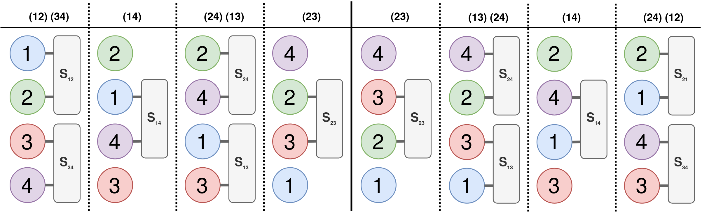
In this work we employ instead the swap-network scheme introduced in Ref. Hall et al. (2021) for studying neutrino dynamics on a digital quantum computer with linear connectivity. The construction is inspired by earlier work on fermionic swap-networks Kivlichan et al. (2018) and relies on the observation that, if we perform layers of nearest-neighbor swap operations by alternating the even bonds with the odd bonds, we can bring every site next to every other site at least once using a total of operations. At the end of these steps, the sites will be left in reverse order. It is now clear that, if we define a modified propagator as follows (with from Eq. (25))
| (29) |
and apply nearest-neighbor operations instead of swaps as before, at the end of the sequence we will have implemented the first product of pair operators in the approximation Eq. (26) for the propagator. If we now apply the sequence in reverse order we can complete a full time step and obtain a state where sites have the original order. One can express this more directly by explicitly denoting the sites where the unitary operation is applied as superscript indices . With this notation, and assuming even for simplicity, we can express the total unitary on the -th even layer and on the -th odd layer as follows
| (30) |
where and denote the amplitude residing on site at the -th even or odd step. The mapping between sites and amplitudes evolves as the algorithm proceeds but it is straightforward to keep track of this and assign the correct amplitude index at every point in the step. The full second-order step from Eq. (26) can then be expressed as
| (31) |
A schematic depiction of a complete step for a system with neutrinos is displayed in Fig. 1. In order to avoid cumbersome notation, in the figure only the lower indices in the propagators are used and these identify the neutrino amplitude associated with the specific sites the propagator is acting upon at any given step.
In this work we perform a SVD truncation to MPS form after each application of the nearest neighbor operation using a threshold of for the discarded eigenvalues. Better truncation schemes are possible (see eg. Paeckel et al. (2019)) and their potential advantages will be explored in future work.
Finally, we decompose the full time evolution for a total time into steps of size as
| (32) |
We then approximate each short-time propagator for time using the swap-network scheme described above.
For all the results presented in the main text, we used a fixed time-step which we found provided a good compromise between precision and efficiency for the systems studied here (see also Appendix A for a more complete discussion). As already mentioned above, the overall scheme remains efficient provided the singular values on each bond decay sufficiently fast to zero that a good approximation to the MPS can be obtained using a low bond dimension. Thanks to the (at most) logarithmic scaling of the entanglement entropy observed in the systems studied in main text, the maximum bond dimension required to keep the truncation error below was allowing us to easily explore systems with . The software developed to carry out the simulations reported in this work used the C++ version of the ITensor library which provides efficient representations for MPS and more general tensors Fishman et al. (2020).
III Results
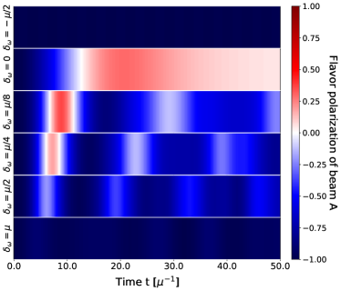
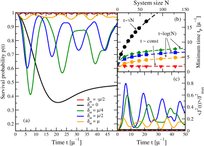
The qualitative difference on the collective flavor oscillations in the different dynamical phases can be observed directly from the time evolution of the flavor polarization. Fig. 2 shows the average flavor polarization of the neutrinos in the beam , for a system of neutrinos and different values for the asymmetry energy . Due to the conservation of , the polarization of beam B is simply the inverse. We can see strong flavor oscillations for which for can even lead to a net flavor inversion in the beam (red areas in Fig. 2). In the stable phases for large values of (bottom panel) or negative asymmetries (top panel), the amplitude of these oscillations is greatly reduced. More detail on these flavor oscillations is given in panel (a) of Fig. 3 where we show the results for the survival probability and the same system of neutrinos. For negative values of the polarization experiences small oscillations around the initial state, as expected from our the discussion on the evolution of the total angular momentum based on Eq. (4).
In the phase with the survival probability experiences instead fast oscillations on time scales much shorter than in the high density limit . If, in the latter case, the first minimum of the survival probability is reached for a time that scales with , in the former case we have instead evolution at the fast scale found in Refs. Bell et al. (2003); Sawyer (2004), but now for a physical model with invariance (see also Roggero (2021)). The difference in scaling of with system size is evident from the results presented in panel (b) of Fig. 3. For all values of a good fit to data is obtained with the ansatz . The best fit values for the parameters extracted from our simulations are reported in Tab. 1, together with the extrapolated value of the minimum of the survival probability in the limit. Even though it doesn’t directly quantify the final flavor content in the long time limit, this quantity is still remarkably useful as it provides an upperbound on the maximum amplitude of flavor oscillations. In particular we see that, for outside the critical region , the latter converges to in the thermodynamic limit and no flavor evolution is present. Interestingly, the fluctuation timescales in the unstable region seem to scale approximately as similarly to the more familiar bipolar oscillations Kostelecký and Samuel (1995); Hannestad et al. (2006); Duan et al. (2007). The instability observed in our simulations is also similar to bipolar oscillations in that, if we take the beam to be composed of anti-neutrinos (with negative Duan et al. (2010) in normal hierarchy) and beam of neutrinos, the appearance of the instability leading to oscillations in our setting depends on the neutrino hierarchy: for inverted hierarchy, the single particle energies change sign and the instability cannot occur because irrespective of the energies, for normal hierarchy we have always positive energy differences and oscillations can occur when . The situation is reversed exchanging neutrinos with anti-neutrinos. Finally, fast oscillations can also occur if both beams are composed by neutrinos (or anti-neutrinos) provided that
| (33) |
with for and for in the normal hierarchy 333Note that this condition can be modified by the presence of an MSW-like matter term which couple differently to the two flavors..
| -0.5 | 0 | 0 | 1.8(2) | 1.00(1) |
| 0.0 | 0 | 2.10(5) | 0 | 0.36(1) |
| 0.01 | 5.4(2) | 0 | -8(1) | 0.35(2) |
| 0.05 | 2.58(6) | 0 | 0 | 0.31(4) |
| 0.125 | 1.65(6) | 0 | 1.4(2) | 0.32(3) |
| 0.25 | 1.22(4) | 0 | 1.6(2) | 0.41(3) |
| 0.5 | 1.06(4) | 0 | 1.4(2) | 0.61(4) |
| 1.0 | 0.96(5) | 0 | 0 | 0.99(2) |
In panel (c) of Fig. 3 we show the, normalized, expectation value of the total angular momentum measured using the relation in Eq. (4) derived above. As we can see from the figure, in the unstable region the system can acquire a considerable fraction of the maximum possible total angular momentum, especially for (blue line) where it reaches a maximum of .
As an alternative way to quantify quantum correlations in the evolved state, we compute the half-chain entanglement entropy (see eg. Eisert et al. (2010)) defined explicitly as
| (34) |
Here the density matrix is obtained by tracing the full density matrix of the system at time over the first neutrinos.
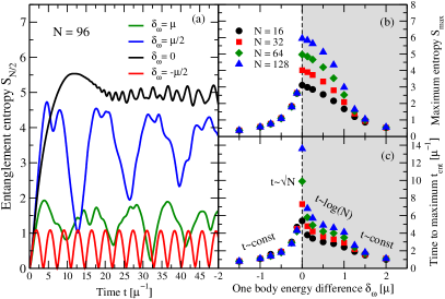
The presence of different dynamical phases can be seen directly from the results on the half-chain entanglement entropy presented in Fig. 4. Panel (b) shows the maximum value that is reached by the entanglement entropy for different values of and system sizes while in panel (a) we show examples of the time evolution of for a system of neutrinos. In the phase for , the behavior is similar to a gapped system with independent of system size while we find to oscillate in time (red curve) with an approximately constant frequency. We recover a similar result for when, as expected from the discussion above, the system becomes again approximately frozen in the initial configuration. As shown in panel (a) for the case (orange line), the oscillations in the entanglement entropy are much less regular than in the phase and do not return close to zero. At the transition point we find that, after an initial rapid growth phase, the entropy reaches a peak at and then plateaus at a slightly smaller value with oscillations around the average. This maximum value for the entanglement entropy is reminiscent to the one in ground states of spin systems at a quantum critical point Vidal et al. (2003); Refael and Moore (2004) and reflects the absence of a gap in the Hamiltonian. This connection allows to understand why it is possible to carry out an efficient simulation even in the infinite interaction range considered here Schuch et al. (2008). We find a similar behavior for the maximum entropy reached in the dynamics for the intermediate regime as shown in panel(b). For non-zero values of the energy asymmetry however, the half-chain entanglement entropy shows strong oscillations analogous to those found in similar spin models undergoing a dynamical phase transition Roggero (2021). We note that an increased dynamics of the entanglement entropy has been already associated in the past to the presence of a dynamical phase transition, but was usually associated with a increase of the time-derivative of at the critical times Heyl (2018); Haldar et al. (2020).
The time needed to reach the first maximum in the entanglement entropy is shown in panel (c) of Fig. 4 and has three distinct scaling regimes: for is approximately independent from system size, at the critical point we recover the familiar and for positive we find a logarithmic evolution which seems to approach a constant again for large value of . In this regime the system seems to enter a second ”gapped” phase, similar to the one for , but simulations with larger systems might be required to confirm this.
IV Summary and Perspective
Entanglement is a fundamental feature of interacting quantum many body systems Vidal et al. (2003); Eisert et al. (2010) which, somewhat surprisingly, can be shown to play no important role in determining ground-state properties of systems with all-to-all interactions like for the neutrino forward-scattering Hamiltonian of Eq. (1) (see eg. Brandão and Harrow (2016)). This is at the heart of the expectation that a mean-field treatment of the dynamics would also be appropriate. However, the role played by entanglement in out-of-equilibrium settings, like those relevant for flavor evolution in a supernova environment, is not as well understood Cervia et al. (2019); Rrapaj (2020).
In this work we have solved for the real time dynamics of a simpler system described by the Hamiltonian in Eq. (2) sharing many similarities to the model used to describe bipolar oscillations Hannestad et al. (2006); Duan et al. (2010). In order to overcome the exponential complexity of a direct solution of the problem we use a simple technique, based on a MPS representation Vidal (2003), whose computational complexity scales with the amount of entanglement generated by the dynamics. The results for this simple model suggest that the maximum bipartite entropy reached in collective neutrino oscillations scales only as with the logarithm of the system size. This favorable scaling allows for the efficient calculation of the dynamics for relatively long times and systems exceeding neutrinos. The computational efficiency could also be improved by using more complex tensor networks like MERA Vidal (2008) which naturally describe states with logarithmically increasing entropy.
As shown in an accompanying paper Roggero (2021), the behavior observed here is also found in similar (non-integrable) spin systems whose out-of-equilibrium dynamics crosses a quantum critical point, suggesting a strong link between dynamical phase transitions and fast collective oscillations. This link provides us directly with conditions, like Eq. (33), to determine when instabilities can occur. These conditions provide a generalization of those commonly obtained with linear stability analysis to the long time, non-linear, regime.
The artificial setting considered here, with a strongly asymmetric initial state and no effect from the vacuum mixing angle, was chosen to highlight differences with a typical mean-field treatment of the problem where the dynamics is simply absent. We expect however the qualitative conclusions reached here, fast oscillations caused by a dynamical phase transition and a general slow growth of the entanglement entropy with system size, to be valid also in more general situations where multi-angle effects, and more complicated energy distributions are considered Roggero (2021). In this regime, MPS simulations could be used reliably to track flavor dynamics up to relatively large, and more realistic, neutrino systems. Important extensions of this work will be to include effects due to finite-mixing angles, the interaction with external matter, the generalization to the 3 flavor case and the more realistic time-dependent setting.
Based on the results presented here, we still cannot completely exclude the existence of neutrino configurations able to generate substantially more entanglement during the dynamics. Interestingly, the presence of these classically-hard configurations would be signalled clearly by the failure of the MPS method to scale efficiently to large system sizes. If found, these would be ideal models to explore using near-term quantum simulators like trapped-ion systems Zhang et al. (2017) or future circuit based quantum computers Hall et al. (2021), which do not necessarily suffer from an exponentially increasing computational cost when large entanglement is present. In future studies, the effects discussed here will be integrated into more realistic simulations to better ascertain the role of entanglement in the dynamical evolution of dense neutrino environments of astrophysical importance.
Acknowledgements.
I want to thank Joseph Carlson, Vincenzo Cirigliano, Huaiyu Duan, Joshua Martin, Amol Patwardhan, Ermal Rrapaj and Martin Savage for the many useful discussions about the subject of this work. This work was supported by the InQubator for Quantum Simulation under U.S. DOE grant No. DE-SC0020970 and by the Quantum Science Center (QSC), a National Quantum Information Science Research Center of the U.S. Department of Energy (DOE).References
- Hoffman et al. (1997) R. D. Hoffman, S. E. Woosley, and Y.-Z. Qian, “Nucleosynthesis in neutrino-driven winds. II. implications for heavy element synthesis,” The Astrophysical Journal 482, 951–962 (1997).
- Janka (2012) Hans-Thomas Janka, “Explosion mechanisms of core-collapse supernovae,” Annual Review of Nuclear and Particle Science 62, 407–451 (2012).
- Winteler et al. (2012) C. Winteler, R. Käppeli, A. Perego, A. Arcones, N. Vasset, N. Nishimura, M. Liebendörfer, and F.-K. Thielemann, “MAGNETOROTATIONALLY DRIVEN SUPERNOVAE AS THE ORIGIN OF EARLY GALAXY r-PROCESS ELEMENTS?” The Astrophysical Journal 750, L22 (2012).
- Wanajo et al. (2014) Shinya Wanajo, Yuichiro Sekiguchi, Nobuya Nishimura, Kenta Kiuchi, Koutarou Kyutoku, and Masaru Shibata, “PRODUCTION OF ALL THE r-PROCESS NUCLIDES IN THE DYNAMICAL EJECTA OF NEUTRON STAR MERGERS,” The Astrophysical Journal 789, L39 (2014).
- Savage et al. (1991) Martin J. Savage, Robert A. Malaney, and George M. Fuller, “Neutrino Oscillations and the Leptonic Charge of the Universe,” Astrophys. J. 368, 1 (1991).
- Pantaleone (1992a) James Pantaleone, “Dirac neutrinos in dense matter,” Phys. Rev. D 46, 510–523 (1992a).
- Pantaleone (1992b) James Pantaleone, “Neutrino oscillations at high densities,” Physics Letters B 287, 128 – 132 (1992b).
- Pastor and Raffelt (2002) Sergio Pastor and Georg Raffelt, “Flavor oscillations in the supernova hot bubble region: Nonlinear effects of neutrino background,” Phys. Rev. Lett. 89, 191101 (2002).
- Balantekin and Yüksel (2005) A B Balantekin and H Yüksel, “Neutrino mixing and nucleosynthesis in core-collapse supernovae,” New Journal of Physics 7, 51–51 (2005).
- Fuller and Qian (2006) George M. Fuller and Yong-Zhong Qian, “Simultaneous flavor transformation of neutrinos and antineutrinos with dominant potentials from neutrino-neutrino forward scattering,” Phys. Rev. D 73, 023004 (2006).
- Duan et al. (2006a) Huaiyu Duan, George M. Fuller, J. Carlson, and Yong-Zhong Qian, “Coherent development of neutrino flavor in the supernova environment,” Phys. Rev. Lett. 97, 241101 (2006a).
- Friedland (2010) Alexander Friedland, “Self-refraction of supernova neutrinos: Mixed spectra and three-flavor instabilities,” Phys. Rev. Lett. 104, 191102 (2010).
- Martin et al. (2020) Joshua D. Martin, Changhao Yi, and Huaiyu Duan, “Dynamic fast flavor oscillation waves in dense neutrino gases,” Physics Letters B 800, 135088 (2020).
- Wu and Tamborra (2017) Meng-Ru Wu and Irene Tamborra, “Fast neutrino conversions: Ubiquitous in compact binary merger remnants,” Phys. Rev. D 95, 103007 (2017).
- Fogli et al. (2007) Gianluigi Fogli, Eligio Lisi, Antonio Marrone, and Alessandro Mirizzi, “Collective neutrino flavor transitions in supernovae and the role of trajectory averaging,” Journal of Cosmology and Astroparticle Physics 2007, 010–010 (2007).
- Qian et al. (1993) Yong-Zhong Qian, George M. Fuller, Grant J. Mathews, Ron W. Mayle, James R. Wilson, and S. E. Woosley, “Connection between flavor-mixing of cosmologically significant neutrinos and heavy element nucleosynthesis in supernovae,” Phys. Rev. Lett. 71, 1965–1968 (1993).
- Qian and Fuller (1995) Yong-Zhong Qian and George M. Fuller, “Neutrino-neutrino scattering and matter-enhanced neutrino flavor transformation in supernovae,” Phys. Rev. D 51, 1479–1494 (1995).
- Duan and Friedland (2011) Huaiyu Duan and Alexander Friedland, “Self-induced suppression of collective neutrino oscillations in a supernova,” Phys. Rev. Lett. 106, 091101 (2011).
- Dasgupta et al. (2012) Basudeb Dasgupta, Evan P. O’Connor, and Christian D. Ott, “Role of collective neutrino flavor oscillations in core-collapse supernova shock revival,” Phys. Rev. D 85, 065008 (2012).
- Sawyer (2005) R. F. Sawyer, “Speed-up of neutrino transformations in a supernova environment,” Phys. Rev. D 72, 045003 (2005).
- Sawyer (2016) R. F. Sawyer, “Neutrino cloud instabilities just above the neutrino sphere of a supernova,” Phys. Rev. Lett. 116, 081101 (2016).
- Chakraborty et al. (2016a) S. Chakraborty, R. S. Hansen, I. Izaguirre, and G.G. Raffelt, “Self-induced neutrino flavor conversion without flavor mixing,” Journal of Cosmology and Astroparticle Physics 2016, 042–042 (2016a).
- Izaguirre et al. (2017) Ignacio Izaguirre, Georg Raffelt, and Irene Tamborra, “Fast pairwise conversion of supernova neutrinos: A dispersion relation approach,” Phys. Rev. Lett. 118, 021101 (2017).
- Chakraborty et al. (2016b) Sovan Chakraborty, Rasmus Hansen, Ignacio Izaguirre, and Georg Raffelt, “Collective neutrino flavor conversion: Recent developments,” Nuclear Physics B 908, 366 – 381 (2016b), neutrino Oscillations: Celebrating the Nobel Prize in Physics 2015.
- Vlasenko et al. (2014) Alexey Vlasenko, George M. Fuller, and Vincenzo Cirigliano, “Neutrino quantum kinetics,” Phys. Rev. D 89, 105004 (2014).
- Cirigliano et al. (2015) Vincenzo Cirigliano, George M. Fuller, and Alexey Vlasenko, “A new spin on neutrino quantum kinetics,” Physics Letters B 747, 27–35 (2015).
- Pehlivan et al. (2011) Y. Pehlivan, A. B. Balantekin, Toshitaka Kajino, and Takashi Yoshida, “Invariants of collective neutrino oscillations,” Phys. Rev. D 84, 065008 (2011).
- Note (1) Note the difference in the definition of there.
- Stirner et al. (2018) Tobias Stirner, Günter Sigl, and Georg Raffelt, “Liouville term for neutrinos: flavor structure and wave interpretation,” Journal of Cosmology and Astroparticle Physics 2018, 016–016 (2018).
- Sawyer (2004) R.F. Sawyer, “’Classical’ instabilities and ’quantum’ speed-up in the evolution of neutrino clouds,” (2004), arXiv:hep-ph/0408265 .
- Duan et al. (2010) Huaiyu Duan, George M. Fuller, and Yong-Zhong Qian, “Collective neutrino oscillations,” Annual Review of Nuclear and Particle Science 60, 569–594 (2010), https://doi.org/10.1146/annurev.nucl.012809.104524 .
- Eisert et al. (2015) J. Eisert, M. Friesdorf, and C. Gogolin, “Quantum many-body systems out of equilibrium,” Nature Physics 11, 124–130 (2015).
- Cervia et al. (2019) Michael J. Cervia, Amol V. Patwardhan, A. B. Balantekin, S. N. Coppersmith, and Calvin W. Johnson, “Entanglement and collective flavor oscillations in a dense neutrino gas,” Phys. Rev. D 100, 083001 (2019).
- Rrapaj (2020) Ermal Rrapaj, “Exact solution of multiangle quantum many-body collective neutrino-flavor oscillations,” Phys. Rev. C 101, 065805 (2020).
- Friedland and Lunardini (2003a) Alexander Friedland and Cecilia Lunardini, “Do many-particle neutrino interactions cause a novel coherent effect?” Journal of High Energy Physics 2003, 043–043 (2003a).
- Friedland et al. (2006) Alexander Friedland, Bruce H. J. McKellar, and Ivona Okuniewicz, “Construction and analysis of a simplified many-body neutrino model,” Phys. Rev. D 73, 093002 (2006).
- Bell et al. (2003) Nicole F. Bell, Andrew A. Rawlinson, and R.F. Sawyer, “Speed-up through entanglement—many-body effects in neutrino processes,” Physics Letters B 573, 86 – 93 (2003).
- Note (2) Since we are free to change the intra-beam couplings at will thus changing the geometry. In the general case we can substitute , with the angle between the momenta in the and beams, for all the results in this work.
- Lipkin et al. (1965) H.J. Lipkin, N. Meshkov, and A.J. Glick, “Validity of many-body approximation methods for a solvable model: (i). exact solutions and perturbation theory,” Nuclear Physics 62, 188 – 198 (1965).
- Vidal et al. (2004a) Julien Vidal, Rémy Mosseri, and Jorge Dukelsky, “Entanglement in a first-order quantum phase transition,” Phys. Rev. A 69, 054101 (2004a).
- Vidal et al. (2004b) Julien Vidal, Guillaume Palacios, and Claude Aslangul, “Entanglement dynamics in the lipkin-meshkov-glick model,” Phys. Rev. A 70, 062304 (2004b).
- Vidal et al. (2004c) Julien Vidal, Guillaume Palacios, and Rémy Mosseri, “Entanglement in a second-order quantum phase transition,” Phys. Rev. A 69, 022107 (2004c).
- Latorre et al. (2005) José I. Latorre, Román Orús, Enrique Rico, and Julien Vidal, “Entanglement entropy in the lipkin-meshkov-glick model,” Phys. Rev. A 71, 064101 (2005).
- Ribeiro et al. (2008) Pedro Ribeiro, Julien Vidal, and Rémy Mosseri, “Exact spectrum of the lipkin-meshkov-glick model in the thermodynamic limit and finite-size corrections,” Phys. Rev. E 78, 021106 (2008).
- Friedland and Lunardini (2003b) Alexander Friedland and Cecilia Lunardini, “Neutrino flavor conversion in a neutrino background: Single- versus multi-particle description,” Phys. Rev. D 68, 013007 (2003b).
- Vidal (2003) Guifré Vidal, “Efficient classical simulation of slightly entangled quantum computations,” Phys. Rev. Lett. 91, 147902 (2003).
- Vidal (2004) Guifré Vidal, “Efficient simulation of one-dimensional quantum many-body systems,” Phys. Rev. Lett. 93, 040502 (2004).
- Paeckel et al. (2019) Sebastian Paeckel, Thomas Köhler, Andreas Swoboda, Salvatore R. Manmana, Ulrich Schollwöck, and Claudius Hubig, “Time-evolution methods for matrix-product states,” Annals of Physics 411, 167998 (2019).
- Schuch et al. (2008) Norbert Schuch, Michael M. Wolf, Frank Verstraete, and J. Ignacio Cirac, “Entropy scaling and simulability by matrix product states,” Phys. Rev. Lett. 100, 030504 (2008).
- Schollwöck (2011) Ulrich Schollwöck, “The density-matrix renormalization group in the age of matrix product states,” Annals of Physics 326, 96 – 192 (2011), january 2011 Special Issue.
- Hall et al. (2021) Benjamin Hall, Alessandro Roggero, Alessandro Baroni, and Joseph Carlson, “Simulation of Collective Neutrino Oscillations on a Quantum Computer,” arXiv e-prints , arXiv:2102.12556 (2021), arXiv:2102.12556 [quant-ph] .
- Verstraete and Cirac (2006) F. Verstraete and J. I. Cirac, “Matrix product states represent ground states faithfully,” Phys. Rev. B 73, 094423 (2006).
- Suzuki (1991) Masuo Suzuki, “General theory of fractal path integrals with applications to many‐body theories and statistical physics,” Journal of Mathematical Physics 32, 400–407 (1991).
- Stoudenmire and White (2010) E M Stoudenmire and Steven R White, “Minimally entangled typical thermal state algorithms,” New Journal of Physics 12, 055026 (2010).
- Kivlichan et al. (2018) Ian D. Kivlichan, Jarrod McClean, Nathan Wiebe, Craig Gidney, Alán Aspuru-Guzik, Garnet Kin-Lic Chan, and Ryan Babbush, “Quantum simulation of electronic structure with linear depth and connectivity,” Phys. Rev. Lett. 120, 110501 (2018).
- Fishman et al. (2020) Matthew Fishman, Steven R. White, and E. Miles Stoudenmire, “The ITensor software library for tensor network calculations,” (2020), arXiv:2007.14822 .
- Roggero (2021) Alessandro Roggero, “Dynamical Phase Transitions in models of Collective Neutrino Oscillations,” arXiv e-prints , arXiv:2103.11497 (2021), arXiv:2103.11497 [hep-ph] .
- Kostelecký and Samuel (1995) V. Alan Kostelecký and Stuart Samuel, “Self-maintained coherent oscillations in dense neutrino gases,” Phys. Rev. D 52, 621–627 (1995).
- Hannestad et al. (2006) Steen Hannestad, Georg G. Raffelt, Günter Sigl, and Yvonne Y. Y. Wong, “Self-induced conversion in dense neutrino gases: Pendulum in flavor space,” Phys. Rev. D 74, 105010 (2006).
- Duan et al. (2007) Huaiyu Duan, George M. Fuller, J. Carlson, and Yong-Zhong Qian, “Analysis of collective neutrino flavor transformation in supernovae,” Phys. Rev. D 75, 125005 (2007).
- Note (3) Note that this condition can be modified by the presence of an MSW-like matter term which couple differently to the two flavors.
- Eisert et al. (2010) J. Eisert, M. Cramer, and M. B. Plenio, “Colloquium: Area laws for the entanglement entropy,” Rev. Mod. Phys. 82, 277–306 (2010).
- Vidal et al. (2003) G. Vidal, J. I. Latorre, E. Rico, and A. Kitaev, “Entanglement in quantum critical phenomena,” Phys. Rev. Lett. 90, 227902 (2003).
- Refael and Moore (2004) G. Refael and J. E. Moore, “Entanglement entropy of random quantum critical points in one dimension,” Phys. Rev. Lett. 93, 260602 (2004).
- Heyl (2018) Markus Heyl, “Dynamical quantum phase transitions: a review,” Reports on Progress in Physics 81, 054001 (2018).
- Haldar et al. (2020) Asmi Haldar, Krishnanand Mallayya, Markus Heyl, Frank Pollmann, Marcos Rigol, and Arnab Das, “Signatures of quantum phase transitions after quenches in quantum chaotic one-dimensional systems,” arXiv e-prints , arXiv:2004.02905 (2020), arXiv:2004.02905 [cond-mat.stat-mech] .
- Brandão and Harrow (2016) Fernando G. S. L. Brandão and Aram W. Harrow, “Product-state approximations to quantum states,” Communications in Mathematical Physics 342, 47–80 (2016).
- Vidal (2008) G. Vidal, “Class of quantum many-body states that can be efficiently simulated,” Phys. Rev. Lett. 101, 110501 (2008).
- Zhang et al. (2017) J. Zhang, G. Pagano, P. W. Hess, A. Kyprianidis, P. Becker, H. Kaplan, A. V. Gorshkov, Z.-X. Gong, and C. Monroe, “Observation of a many-body dynamical phase transition with a 53-qubit quantum simulator,” Nature 551, 601–604 (2017).
- Childs et al. (2021) Andrew M. Childs, Yuan Su, Minh C. Tran, Nathan Wiebe, and Shuchen Zhu, “Theory of trotter error with commutator scaling,” Phys. Rev. X 11, 011020 (2021).
- Duan et al. (2006b) Huaiyu Duan, George M. Fuller, and Yong-Zhong Qian, “Collective neutrino flavor transformation in supernovae,” Phys. Rev. D 74, 123004 (2006b).
- Haegeman et al. (2011) Jutho Haegeman, J. Ignacio Cirac, Tobias J. Osborne, Iztok Pižorn, Henri Verschelde, and Frank Verstraete, “Time-dependent variational principle for quantum lattices,” Phys. Rev. Lett. 107, 070601 (2011).
Appendix A Analysis of time-step errors
In this appendix we provide more information about the choice of time step in the MPS simulations used in the main text. We first recall the expression for the approximate evolution operator used in our simulations
| (35) |
and the very conservative error bound (see e.g. Childs et al. (2021) for tighter ones) presented in Eq. (26) of the main text
| (36) |
where are operator norms. This approximation is then useful for short-time evolutions only and in order to perform accurate simulations for a long time it is necessary to break the interval in small steps of size as described in Eq. (32) of the main text. Using the union bound, one can straightforwardly generalize Eq. (37) to arbitrary long times as follows
| (37) |
This results implies that, for a fixed evolution time , the error scales quadratically with the time step and that to guarantee a maximum error it is sufficient to choose
| (38) |
where is the total number of steps in the simulation.
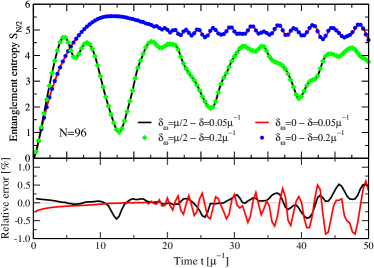
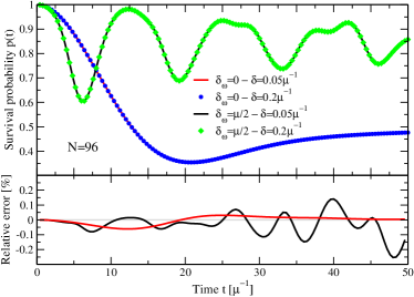
In order to estimate the contribution of this error to the observables displayed in the main text we performed additional simulations for the system at both and using a time step four times larger than the one used for the simulations described in the main text. We show the comparison between these two choices of time step for a system with neutrinos and two values of the energy asymmetry for the entanglement entropy in Fig. 5 and for the survival probability in Fig. 6. The top panels show with continuous lines the results for (the choice used for the results in the main text) and the dots indicate the results with which are expected to have times larger time-step errors. The observed deviations are extremely small for all times and, as shown in the bottom panels of both figures, increase slightly with the total evolution time but are always below for the entanglement entropy and for the survival probability. Importantly, for times close to the maximum of the entropy the errors are well below the percent level indicating that the time step error is not a significant contribution to the uncertainty of the results presented in the main text.
Appendix B Direct comparison with mean-field
In this last section we show results obtained from a direct comparison between the MPS representation used in the work presented in the main text and a more standard mean-field solution of the evolution equations. This is done in order to better elucidate the role of the approximations used in the time-evolution algorithm described in the previous section and of possible finite-size effects which are absent in the mean-field.
The model considered in the main text is in the mass basis and in the mean-field approximation there is no flavor evolution. By rotating the initial state toward the flavor basis one can however produce collective oscillations also within the approximation. In this section, we will compare the flavor evolution in the mean-field approximation and the thermodynamical limit with a MPS simulation at finite where at each time step we truncate the bond dimension to on all links.
For this discussion we will use the same Hamiltonian in Eq.(3) of the main text, but rotated to the flavor basis
| (39) |
with , the total spin operators in the two beams and is related to the mixing angle . In the following, we will also keep the same initial condition as in the text, but now in the flavor basis. The equation of motion for the spin operators can then be expressed as follows
| (40) |
One can eliminate the explicit dependence on the number of amplitudes by expressing these equations in terms of polarization vectors and . In the mean field approximation we have then
| (41) |
The solution of these coupled equations can be simplified with the change of variables proposed in Refs. Duan et al. (2006b); Hannestad et al. (2006).
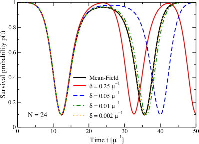
In Fig. 7 we compare the result for the time evolution of the survival probability
| (42) |
as obtained by either solving the equations in Eq. (41) (black solid line) or using the MPS time-evolution scheme described above with a fixed bond dimension of (this figure is equivalent to the solid curve in Fig. 2(b) of Ref. Duan et al. (2006b), upon rescaling of the time variable). The different colored curves correspond to different choices for the time-step used to simulate time-evolution with Eq. (32). The results show a discrepancy with the mean-field results that grows as a function of time and depends on the chosen time-step. This effect is due to the approximate way the evolution is maintained at the mean field level: the local SVD-based truncation of a link tensor to does not guarantee to select the globally optimal tensor. This deficiency of the time evolution scheme described in Sec. II.2 is one of the main motivation behind alternatives like the Time Dependent Variational Principle(TDVP) approach Haegeman et al. (2011) which, instead, approximates globally optimal tensors remaining directly on the manifold of matrix product states with fixed bond dimension. As the operators used in the updates from Eq. (21) become closer to the identity, this truncation error becomes smaller. We can clearly see this effect in Fig. 7 as we lower the size of the time step. These results show the importance of checking convergence of results with respect to the choice of (as done here in Appendix A) and also the potential benefits of incorporating ideas like the TDVP scheme in future studies of neutrino oscillations with MPS.