SuperFaB: a fabulous code for Spherical Fourier-Bessel decomposition

Abstract

The spherical Fourier-Bessel (SFB) decomposition is a natural choice for the radial/angular separation that allows extraction of cosmological information from large volume galaxy surveys, taking into account all wide-angle effects. In this paper we develop a SFB power spectrum estimator that allows the measurement of the largest angular and radial modes with the next generation of galaxy surveys. The code measures the pseudo-SFB power spectrum, and takes into account mask, selection function, pixel window, and shot noise. We show that the local average effect (or integral constraint) is significant only in the largest-scale mode, and we provide an analytical covariance matrix. By imposing boundary conditions at the minimum and maximum radius encompassing the survey volume, the estimator does not suffer from the numerical instabilities that have proven challenging for SFB analyses in the past. The estimator is demonstrated on simplified but realistic Roman-like, SPHEREx-like, and Euclid-like mask and selection functions. For intuition and validation, we also explore the SFB power spectrum in the Limber approximation. We release the associated public code written in Julia.

I Introduction

One of the aims of future galaxy surveys such as the Nancy Grace Roman Space Telescope, SPHEREx, Euclid, DESI, PFS (Spergel et al., 2015; Doré et al., 2014; Amendola et al., 2018; DESI Collaboration et al., 2016; Takada et al., 2014) is to answer questions that require measurement of the galaxy overdensity power spectrum on very large cosmological scales. Chiefly among those is the study of modified theories of gravity (e.g. Munshi et al., 2016) and the measurement of primordial non-Gaussianity that manifests itself in the power spectrum as a scale-dependent galaxy bias $\propto\,k^{-2}$ in the simplest models (Salopek and Bond, 1990; Komatsu and Spergel, 2001; Dalal et al., 2008; Desjacques et al., 2018). However, the measurement of these large scales is not without challenge.

Large angular scales are difficult to exploit fully with a standard 3D power spectrum analysis due to line-of-sight effects such as redshift-space distortions (RSD). When the angular separation between galaxies is large, the assumption that a single line of sight can be used for both galaxies breaks down, which results in a loss of information from the measurement. For example, for a full-sky survey, a fixed LOS estimator is expected to measure a vanishing quadrupole. On medium large scales the problem can be mitigated by choosing a common line of sight for each pair of galaxies (Yamamoto et al., 2006; Bianchi et al., 2015; Scoccimarro, 2015). However, on very large angular scales, we expect that the Yamamoto estimator suffers from the same problem as a fixed-LOS estimator, because at least one of the lines of sight for each galaxy pair is being projected, and that projection likely leads to a loss of information. An optimal power spectrum measurement, therefore, needs to allow for a different line of sight for every galaxy in the survey.

Large radial scales pose a different kind of challenge, and in the past have mostly been treated by splitting surveys into redshift bins (e.g., Beutler et al., 2017). The advantage is that it makes the analysis simple. However, modes larger than the redshift bin are not measured in the radial direction, and that information is lost by such an analysis. (See Zaroubi and Hoffman, 1996, however.)

In this paper, we study and implement a method that enables accurate measurements of the largest radial and angular scales mapped by coming surveys. It relies on the spherical Fourier-Bessel (SFB) transform. Most past measurements of the galaxy overdensity power spectrum rely on Fourier decomposition as it decreases the computation cost of near optimal statistical estimators. While a standard Fourier transform decomposes a field into a linear composition of eigenfunctions to the Laplacian in Cartesian coordinates, the SFB transform we consider does the same but in spherical coordinates. Not only does it maintain the statistical and computational (except for speed) advantages of Fourier methods, but it is also the natural coordinate system for the angular/radial separation over the sphere. The radial line of sight for every single galaxy is built into the method, and the modeling of redshift evolution of galaxy bias and growth factor is straightforward. An overview of the SFB power spectrum is given in Pratten and Munshi (2013) and a mathematical treatment clarifying the relation between the configuration-space correlation function, Fourier space correlation function, SFB correlation function, and mixed-space correlation functions can be found in Reimberg et al. (2016).

The spherical Fourier-Bessel transform for the analysis of galaxy surveys has been considered multiple times in the past. Binney and Quinn (1991) used a SFB decomposition to characterize overdensities deep in the nonlinear regime. Lahav (1993) applied the SFB analysis to local galaxies on larger scales. Heavens and Taylor (1995) applied the SFB analysis to the IRAS 1.2-Jy galaxy catalogue, Tadros et al. (1999) applied it to the PSCz galaxy catalogue, and Percival et al. (2004) use it in the context of the 2dF Galaxy Redshift Survey. Leistedt et al. (2012) have provided a public SFB code, 3DEX, that performs the SFB decomposition first in the radial direction for each galaxy individually, then performs the angular transform using HEALPix. More recently, Wang et al. (2020) have built a combined SFB/$P(k)$ estimation code that uses SFB on very large scales, and a Cartesian multipole power spectrum estimator on smaller scales.

SFB power spectrum measurements tended to be plagued by numerical instabilities and computational complexity. The source of the numerical instability is the incomplete coverage of the analysis volume by the survey. For example, typically a boundary condition is applied at some distance $r_{\mathrm{max}}$, and the analysis is performed for the entire volume inside a sphere of radius $r_{\mathrm{max}}$. However, most surveys will leave most of that volume unexplored, and the de-convolution of the window function or the inversion of the covariance matrix become numerically unstable (e.g., see Wang et al., 2020, for a solution). The numerical complexity stems from the large number of modes that need to be calculated even when a large fraction of the analysis volume remains empty. Another source of computational complexity is the combined estimation of the real-space power spectrum and redshift-space distortion parameters that requires repeated estimations of the power spectrum (Wang et al., 2020).

The spherical Fourier Bessel decomposition code presented in this paper, SuperFaB, combines several approaches to address these problems. For the first time, we limit the redshift range by introducing a boundary condition at $r_{\mathrm{min}}$ as suggested by Samushia (2019). We also use the 3DEX approach by Leistedt et al. (2012) that does not suffer from pixel window effects in the radial direction. The 3DEX approach also allows separation of the angular and radial transforms, and for the angular transform we use HEALPix (Górski et al., 2005; Zonca et al., 2019). Our bandpower binning is done similar to that for CMB measurements (Hivon et al., 2002; Alonso et al., 2019), should a window-decoupled SFB power spectrum be desired, e.g., for comparison with other surveys. We test our code on Roman-like, SPHEREx-like, and Euclid-like survey simulations with $\sim 6\sim 70$ million galaxies per simulation.

In our approach the SFB power spectrum is measured directly, and parameter estimation is left as a second step in the analysis pipeline (to be developed in a future paper). Evolution with redshift of parameters or the power spectrum is encoded in the SFB power spectrum itself. Thus, our vision is to construct the likelihood with parameters modeling the deviations from a reference cosmology. For example, the deviation of the distance-redshift relation would be modeled as a low-order polynomial relative to the reference $r_{\mathrm{ref}}(z)$ so that the true distance is $r_{\mathrm{true}}(z)=\left(a_{0}+a_{1}\,r_{\mathrm{ref}}(z)\right)r_{\mathrm{ref}}(z)$, and parameters $a_{0}$ and $a_{1}$ are to be measured.

An alternative to the SFB analysis that also naturally performs the angular/radial separation is spherical harmonic tomography (SHT, see e.g. Camera et al., 2018; Nicola et al., 2014) where an angular spherical harmonic analysis is performed on shells of redshift bins. Lanusse et al. (2015) conclude that SFB yields similar constraints as SHT, but when it comes to marginalizing over systematic biases such as evolving scale-dependent galaxy bias, SFB performs better. Additionally, Castorina and White (2018) developed various approaches to incorporating wide-angle effects in Fourier based estimators. Beutler et al. (2019) implement a small-angle expansion for the standard multipole power spectrum.

Another point to be made about the choice of the SFB basis is that RSD are readily modeled (see Eq.(16) in Heavens and Taylor, 1995), because they are ultimately sourced by the gravitational potential described by Poisson’s equation.

In Section II we review the SFB power spectrum and develop intuition in the Limber approximation. Section III details the approach taken for the SFB decomposition, window de-convolution, shot noise, bandpower binning, local average effect, and covariance matrix. We show comparisons with log-normal simulations in Section IV for Roman, SPHEREx, and Euclid, and we conclude in Section V. We leave to the appendices a collection of useful formulae in Appendix A, review the Laplacian in an expanding universe in Appendix B, derive the radial potential boundary conditions in Appendix D, and simplify the covariance matrix in Appendices E and F. Our SuperFaB code is publically available at https://github.com/hsgg/SphericalFourierBesselDecompositions.jl.

II SFB Power Spectrum

In this section we briefly review the SFB formalism. We start with the basic transformation between configuration space and SFB space as well as between Fourier space and SFB space. We then briefly show the power spectrum in a completely homogeneous and isotropic universe before adding in selection function, linear growth factor, galaxy bias, and RSD. We develop intuition by applying Limber’s approximation.

The spherical Fourier-Bessel decomposition expresses a field $\delta({\bm{r}})$ in terms of eigenfunctions of the Laplacian in spherical coordinates. For more details, we refer the reader to Section III.1. We define the spherical Fourier-Bessel modes $\delta_{\ell m}(k)$ by

$$\delta({\bm{r}}) =\int\mathrm{d}k\,\sum_{\ell m}\left[\sqrt{\frac{2}{\pi}}\,k\,j_{\ell}(kr)\,Y_{\ell m}(\theta,\phi)\right]\delta_{\ell m}(k)\,,$$ (1)

$$\delta_{\ell m}(k) =\int\mathrm{d}^{3}r\left[\sqrt{\frac{2}{\pi}}\,k\,j_{\ell}(kr)\,Y^{*}_{\ell m}({\hat{\bm{r}}})\right]\delta({\bm{r}})\,,$$ (2)

where ${\bm{r}}=r{\hat{\bm{r}}}$ is the position vector, $r$ is the comoving angular diameter distance from the origin, and ${\hat{\bm{r}}}$ is the direction on the sky. Here, we assume that the universe is approximately flat. If the curvature is significant, then the spherical Bessels need to be replaced by ultra-spherical Bessels (Abbott and Schaefer, 1986; Zaldarriaga and Seljak, 2000; Kitching et al., 2007). The orthogonality relations Eqs. 109 and 110 for the spherical Bessel functions and spherical harmonics are used to prove that Eqs. 1 and 2 are inverses of each other. The factor $2k^{2}/\pi$ can be split between Eqs. 1 and 2 as pleased. Here we use the convention in Nicola et al. (2014), because for a non-evolving, homogeneous, and isotropic universe the SFB power spectrum then equals $P(k)$, see Eq. 7 below.

The relation between the SFB coefficients $\delta_{\ell m}(k)$ and the Fourier modes $\delta({\bm{k}})$ is obtained by expressing $\delta({\bm{r}})$ in terms of its Fourier transform in Eq. 2,

$$\delta_{\ell m}(k) =\sqrt{\frac{2}{\pi}}\,k\int\mathrm{d}^{3}r\,j_{\ell}(kr)\,Y^{*}_{\ell m}({\hat{\bm{r}}})\int\frac{\mathrm{d}^{3}q}{(2\pi)^{3}}\,e^{i{\bm{q}}\cdot{\bm{r}}}\,\delta({\bm{q}})\,.$$ (3)

With Rayleigh’s formula Eq. 113 this turns into

$$\delta_{\ell m}(k) =\int\frac{\mathrm{d}^{3}q}{(2\pi)^{3}}\,\sqrt{\frac{\pi}{2q^{2}}}\,4\pi\sum_{\ell^{\prime}m^{\prime}}i^{\ell^{\prime}}\,Y^{*}_{\ell^{\prime}m^{\prime}}({\hat{\bm{q}}})\,\delta({\bm{q}})$$

$$\quad\times\frac{2kq}{\pi}\int\mathrm{d}{r}\,r^{2}\,j_{\ell}(kr)\,j_{\ell^{\prime}}(qr)$$

$$\quad\times\int\mathrm{d}^{2}{\hat{\bm{r}}}\,Y^{*}_{\ell m}({\hat{\bm{r}}})\,Y_{\ell^{\prime}m^{\prime}}({\hat{\bm{r}}})$$

$$=\frac{k}{(2\pi)^{\frac{3}{2}}}\,i^{\ell}\int\mathrm{d}^{2}{\hat{\bm{k}}}\,Y^{*}_{\ell m}({\hat{\bm{k}}})\,\delta({\bm{k}})\,,$$ (4)

where the orthogonality relations Eqs. 109 and 110 were used. Eq. 4 shows that SFB is a spherical harmonic transform of Cartesian Fourier modes with an additional phase factor $i^{\ell}$. And

$$\delta({\bm{k}}) =\frac{(2\pi)^{\frac{3}{2}}}{k}\sum_{\ell m}i^{-\ell}\,Y_{\ell m}({\hat{\bm{k}}})\,\delta_{\ell m}(k)$$ (5)

is the inverse of Eq. 4.

II.1 The Homogeneous and Isotropic Universe

In a homogeneous and isotropic universe in real-space (with no line-of-sight effects), we have

$$\left\langle\delta({\bm{k}})\,\delta^{*}({\bm{k}}^{\prime})\right\rangle =(2\pi)^{3}\delta^{D}({\bm{k}}-{\bm{k}}^{\prime})\,P(k)\,.$$ (6)

Therefore, applying Eq. 4 gives the SFB power spectrum as

$$\left\langle\delta_{\ell m}(k)\,\delta^{*}_{\ell^{\prime}m^{\prime}}(k^{\prime})\right\rangle =\delta^{D}(k-k^{\prime})\,\delta^{K}_{\ell\ell^{\prime}}\,\delta^{K}_{mm^{\prime}}\,P(k)\,,$$ (7)

where we used Eq. 107 for the three-dimensional Dirac-delta function in spherical coordinates. That is, in a homogeneous and isotropic universe with no observational effects the SFB power spectrum equals the 3D power spectrum $P(k)$.

II.2 The Linear Universe

We now generalize to include line-of-sight effects, a linearly evolving power spectrum, and a radial window function. The galaxy density contrast we consider is

$$\delta^{\mathrm{obs}}_{g}({\bm{r}}) =W({\bm{r}})\,D(r)\int\frac{\mathrm{d}^{3}q}{(2\pi)^{3}}\,e^{i{\bm{q}}\cdot{\bm{r}}}\,\widetilde{A}_{\mathrm{RSD}}(\mu,q\mu,r)$$

$$\quad\times b(r,q)\,\delta({\bm{q}})\,,$$ (8)

where $\delta({\bm{q}})$ is the matter density contrast in Fourier space, $W({\bm{r}})$ is the survey window function, $D(r)$ is the linear growth factor, $b(r,q)$ is the possibly scale-dependent linear galaxy bias, $\mu={\hat{\bm{q}}}\cdot{\hat{\bm{r}}}$, and the redshift-space distortions are encoded in (e.g., Kaiser, 1987; Grasshorn Gebhardt and Jeong, 2020)

$$\widetilde{A}_{\mathrm{RSD}}(\mu,q\mu,r)=\left(1+\beta\mu^{2}\right)\widetilde{A}_{\mathrm{FoG}}(q\mu)\,,$$ (9)

with $\beta=f/b$, where $f=\mathrm{d}\ln D/\mathrm{d}\ln a$ is the linear growth rate, and we assume a Gaussian fingers-of-God term (Peacock and Dodds, 1994)

$$\widetilde{A}_{\mathrm{FoG}}(q\mu) =e^{-\frac{1}{2}\sigma_{u}^{2}q^{2}\mu^{2}}\,,$$ (10)

with $\sigma_{u}=\sigma_{v}/aH$ the pair-wise velocity dispersion in units of length. The tilde on $A_{\mathrm{RSD}}$ signifies that it is a Fourier-space function.

The RSD term $\widetilde{A}_{\mathrm{RSD}}$ in Section II.2 can be expressed as a function of derivatives on the complex exponential. That is, by performing a Taylor series expansion we can replace $\mu\to-i\partial_{qr}$, or

$$\widetilde{A}_{\mathrm{RSD}}(\mu,q\mu,r)\,e^{i{\bm{q}}\cdot{\bm{r}}} =\sum_{n}\frac{a_{n}(q,r)}{n!}\,\mu^{n}\,e^{iqr\mu}$$

$$=\sum_{n}\frac{a_{n}(q,r)}{n!}\left(-i\,\frac{\partial}{\partial(qr)}\right)^{n}\,e^{iqr\mu}$$

$$=\widetilde{A}_{\mathrm{RSD}}(-i\partial_{qr},-iq\partial_{qr},r)\,e^{i{\bm{q}}\cdot{\bm{r}}}\,.$$ (11)

Furthermore, the complex exponential is expanded using Rayleigh’s formula Eq. 113 so that the derivatives in $\widetilde{A}_{\mathrm{RSD}}$ only act on the spherical Bessel function from Rayleigh’s formula. Further expressing the Fourier-space density contrast in terms of its SFB modes Eq. 5, the observed density contrast Section II.2 now becomes

$$\delta^{\mathrm{obs}}_{g}({\bm{r}}) =W({\bm{r}})\,D(r)\int\frac{\mathrm{d}^{3}q}{(2\pi)^{3}}\,b(r,q)\left[\widetilde{A}_{\mathrm{RSD}}(-i\partial_{qr},-iq\partial_{qr},r)\,4\pi\sum_{L_{1}M_{1}}i^{L_{1}}j_{L_{1}}(qr)\,Y^{*}_{L_{1}M_{1}}({\hat{\bm{q}}})\,Y_{L_{1}M_{1}}({\hat{\bm{r}}})\right]$$

$$\quad\times\frac{(2\pi)^{\frac{3}{2}}}{q}\sum_{LM}i^{-L}\,Y_{LM}({\hat{\bm{q}}})\,\delta_{LM}(q)$$ (12)

$$=W({\bm{r}})\,D(r)\,\sqrt{\frac{2}{\pi}}\int\mathrm{d}q\,q^{2}\,b(r,q)\left[\widetilde{A}_{\mathrm{RSD}}(-i\partial_{qr},-iq\partial_{qr},r)\,\sum_{LM}j_{L}(qr)\,Y_{LM}({\hat{\bm{r}}})\right]\,\frac{1}{q}\,\delta_{LM}(q)\,.$$ (13)

Using Eq. 2 to transform into SFB space,

$$\delta^{g,\mathrm{obs}}_{\ell m}(k) =\int\mathrm{d}q\sum_{LM}\mathcal{W}_{\ell m}^{LM}(k,q)\,\delta_{LM}(q)\,,$$ (14)

where

$$\mathcal{W}_{\ell m}^{LM}(k,q) =\int\mathrm{d}^{2}{\hat{\bm{r}}}\,Y_{LM}({\hat{\bm{r}}})\,Y^{*}_{\ell m}({\hat{\bm{r}}})\,\mathcal{W}_{\ell}^{L}(k,q,{\hat{\bm{r}}})\,,$$ (15)

and

$$\mathcal{W}_{\ell}^{L}(k,q,{\hat{\bm{r}}}) =\frac{2qk}{\pi}\int\mathrm{d}r\,r^{2}\,W({\bm{r}})\,D(r)\,b(r,q)\,j_{\ell}(kr)$$

$$\quad\times\widetilde{A}_{\mathrm{RSD}}(-i\partial_{qr},-iq\partial_{qr},r)j_{L}(qr)\,.$$ (16)

The SFB correlation function is, therefore,

$$\left\langle\delta^{g,\mathrm{obs}}_{\ell m}(k)\,\delta^{g,\mathrm{obs},*}_{\ell^{\prime}m^{\prime}}(k^{\prime})\right\rangle$$

$$=\int\mathrm{d}q\sum_{LM}\mathcal{W}_{\ell m}^{LM}(k,q)\,\mathcal{W}_{\ell^{\prime}m^{\prime}}^{LM,*}(k^{\prime},q)\,P(q)\,,$$ (17)

where we used Eqs. 7 and 14.

Here we will only consider a radial selection function, as the angular mask will be handled in the estimator. Then,

$$W({\bm{r}}) =\phi(r)\,,$$ (18)

and we define the simplification of Section II.2

$$\mathcal{W}_{\ell}(k,q) =\mathcal{W}_{\ell}^{\ell}(k,q,{\hat{\bm{r}}})\,,$$ (19)

which is then independent of the direction ${\hat{\bm{r}}}$. Eq. 15 and Eq. 17 then simplify to

$$\left\langle\delta^{g,\mathrm{obs}}_{\ell m}(k)\,\delta^{g,\mathrm{obs},*}_{\ell^{\prime}m^{\prime}}(k^{\prime})\right\rangle =\delta^{K}_{\ell\ell^{\prime}}\delta^{K}_{mm^{\prime}}\,C_{\ell}(k,k^{\prime})\,,$$ (20)

with the SFB power spectrum defined as

$$C_{\ell}(k,k^{\prime}) =\int\mathrm{d}q\,\mathcal{W}_{\ell}(k,q)\,\mathcal{W}^{*}_{\ell}(k^{\prime},q)\,P(q)\,.$$ (21)

Sections II.2, 19 and 21 show that RSD and linear growth can be taken into account by a change in the radial window function.

Eq. 20 shows that the SFB power spectrum is non-zero only when $\ell=\ell^{\prime}$, $m=m^{\prime}$, and it is independent of $m$. This is a consequence of the isotropy on the sky, or the rotational invariance around the observer, as can be easily shown in general for spherical harmonic transforms.

For a homogeneous and isotropic universe without selection function, $W({\bm{r}})=D(r)=\widetilde{A}_{\mathrm{RSD}}=1$ and $b(r,q)=\mathrm{const}$, the window becomes $\mathcal{W}_{\ell}(k,q)\,\propto\,\delta^{D}(k-q)$, and Eq. 7 is reproduced. Also, $\mathcal{W}_{\ell}(k,q)$ is real, because the imaginary arguments to $\widetilde{A}_{\mathrm{RSD}}$ are only ever raised to even powers.

To develop some intuition for Eq. 21 we evaluate the SFB power spectrum in a Limber-like approximation. However, we defer to Appendix C in order not to distract from the main content of this paper. Other treatments are in Munshi et al. (2016); Yoo and Desjacques (2013).

III SFB Decomposition

This section describes our SFB decomposition for a galaxy survey with mask and selection function. We largely follow Samushia (2019) for the radial basis functions and Leistedt et al. (2012) for the angular/radial split in the estimator.

We start by giving a review of the basis functions, then we add window and selection functions, we model the discrete galaxy distribution, and estimate the covariance matrix.

III.1 Spherical Fourier-Bessel basis with potential boundary conditions

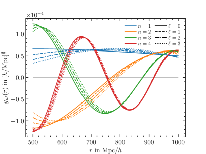
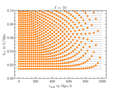
Figure 1: Left: The radial basis functions for potential boundary conditions as a function of $r$. Color indicates the modes $n$, line style indicates $\ell$ as shown in the legend. Here, $r_{\mathrm{min}}=$500\text{\,}{\mathrm{\text{$h$}}}^{-1}\text{\,}\mathrm{Mpc}$$ and $r_{\mathrm{max}}=$1000\text{\,}{\mathrm{\text{$h$}}}^{-1}\text{\,}\mathrm{Mpc}$$. Right: $k_{n\ell}$ for potential boundary conditions as a function of $r_{\mathrm{min}}$ when $\ell=10$. The grey lines are for $r_{\mathrm{min}}=0$, and we fix $r_{\mathrm{max}}=$1000\text{\,}{\mathrm{\text{$h$}}}^{-1}\text{\,}\mathrm{Mpc}$$.

We choose the eigenbasis of the Laplacian as it captures the rotational invariance of the observed large-scale structure, and that leads to a compressed summary statistic which is also rotationally invariant while including all wide-angle effects. Here, we lay out the boundary conditions we consider similar to Samushia (2019). However, as observers fixed in one location, using light that travels at a finite speed, it is more natural to use spherical polar coordinates that separate the radial and angular observations. Then, the Laplacian on a scalar function $f$ becomes

$$\nabla^{2}f =\frac{1}{r^{2}}\,\frac{\partial}{\partial r}\left(r^{2}\,\frac{\partial f}{\partial r}\right)+\frac{1}{r^{2}\sin\theta}\,\frac{\partial}{\partial\theta}\left(\sin\theta\,\frac{\partial f}{\partial\theta}\right)$$

$$\quad+\frac{1}{r^{2}\sin^{2}\theta}\,\frac{\partial^{2}f}{\partial\phi^{2}}\,,$$ (22)

where $r$, $\theta$, and $\phi$ are the comoving angular diameter distance, zenith angle, and azimuthal angle, respectively (see Appendix B for a derivation). The eigenbasis to Eq. 22 that satisfies

$$\nabla^{2}f =-k^{2}f$$ (23)

for some mode $k$ is of the form (see e.g. Samushia, 2019)

$$f_{\ell\mu}(k;r,\theta,\phi) =\big{[}c_{j}\,j_{\ell}(kr)+c_{y}\,y_{\ell}(kr)\big{]}$$

$$\quad\times\big{[}c_{p}\,P_{\ell}^{\mu}(\cos\theta)+c_{q}\,Q_{\ell}^{\mu}(\cos\theta)\big{]}$$

$$\quad\times\big{[}c_{+}\,e^{i\mu\phi}+c_{-}\,e^{-i\mu\phi}\big{]}\,,$$ (24)

where the $c_{i}$ are constants, and $j_{\ell}$ and $y_{\ell}$ are spherical Bessel functions of the first and second kind, and $P_{\ell}^{\mu}$ and $Q_{\ell}^{\mu}$ are Legendre functions of the first and second kind.

The constants $c_{i}$ are set by boundary conditions. First, the spherical Bessel of the second kind, $y_{\ell}$ diverges with vanishing argument; hence, typically $c_{y}=0$. Typically, the functions also need to be periodic about the azimuthal angle $\phi$; therefore, $\mu=0,1,2,\ldots$ is an integer. Then, the functions also need to be finite for $\cos\theta=\pm 1$, typically; therefore, $c_{q}=0$, and $\ell=0,1,2,\ldots$ is an integer, and $-\ell\leq\mu\leq\ell$.

Effectively, the preceding paragraph imposed boundary conditions at $r_{\mathrm{min}}=0$ and assumed coverage of the whole sky. Typically (e.g., Heavens and Taylor, 1995; Fisher et al., 1995; Tadros et al., 1999; Percival et al., 2004), one would then go ahead and also impose boundary conditions at some $r_{\mathrm{max}}$ such that the survey volume is contained within a sphere of radius $r_{\mathrm{max}}$. This restricts the SFB volume, i.e., the volume on which the SFB transform is performed, as the region from $0\leq r\leq r_{\mathrm{max}}$. Demanding the basis functions to be orthogonal then leads to a discrete spectrum of modes $k=k_{n\ell}$.

Realistic galaxy surveys do not occupy the entire SFB volume, but are restricted in both redshift and angular area, and, therefore, they leave large fractions of the SFB volume unobserved. This leads to the deconvolution of the window function to be numerically unstable. It also results in wasted computational resources if the survey covers only a (potentially thick) shell at high redshift. The analogous picture for a standard Fourier transform would be to have a transform box that is much larger than the survey volume. Therefore, the selection function will vanish for part of the SFB volume, and, because in that case some modes are not well constrained, the inversion of the window function becomes numerically unstable.

In this paper, we employ two strategies to deal with this problem. First, we follow Hivon et al. (2002); Alonso et al. (2019) and bin the pseudo SFB power spectrum into bandpowers. This combines several poorly-constrained modes into one well-constrained mode. We rely on this strategy especially for the angular mask so that we can leverage the full-sky spherical harmonic algorithms from the HealPy software (Górski et al., 2005; Zonca et al., 2019).

For the second strategy, we follow Samushia (2019) and move the boundary at the origin to some $r_{\mathrm{min}}$ so that the SFB volume extends from $r_{\mathrm{min}}\leq r\leq r_{\mathrm{max}}$. For galaxy surveys that start at some minimum redshift this eliminates from the SFB tranform volume a hole around the origin. As a result, the inversion of the window function is numerically well behaved even without resorting to bandpower binning. Furthermore, the number of SFB modes is reduced not just by the boundary condition at $r_{\mathrm{max}}$, but the boundary condition at $r_{\mathrm{min}}$ also reduces the number of modes further by the fraction $r_{\mathrm{min}}^{3}/r_{\mathrm{max}}^{3}$. In all cases considered in this paper, this eliminates the need for bandpower binning in the radial direction.

We differ from Samushia (2019) in that we use potential boundary conditions (Fisher et al., 1995) that ensure the field represented by the SFB decomposition is continuous and smooth at the boundary. These boundary conditions lead to a spectrum of modes $k_{n\ell}$, as shown in Appendix D. In the appendix we also derive that the radial basis functions with such boundary conditions become a linear combination of spherical Bessels of the first and second kind,

$$g_{n\ell}(r) =c_{n\ell}\,j_{\ell}(k_{n\ell}\,r)+d_{n\ell}\,y_{\ell}(k_{n\ell}\,r)\,,$$ (25)

which satisfy an orthonormality relation

$$\int_{r_{\mathrm{min}}}^{r_{\mathrm{max}}}\mathrm{d}r\,r^{2}\,g_{n\ell}(r)\,g_{n^{\prime}\ell}(r) =\delta^{K}_{nn^{\prime}}\,,$$ (26)

where $\delta^{K}_{nn^{\prime}}$ is a Kronecker delta, and the coefficients $c_{n\ell}$ and $d_{n\ell}$ are derived in Appendix D. With Eq. 26, the Fourier pair Eqs. 1 and 2 remains a Fourier pair with the discrete $k_{n\ell}$-spectrum, and the pair becomes

$$\delta({\bm{r}}) =\sum_{n\ell m}\Big{[}g_{n\ell}(r)\,Y_{\ell m}({\hat{\bm{r}}})\Big{]}\delta_{n\ell m}\,,$$ (27)

$$\delta_{n\ell m} =\int\mathrm{d}^{3}{\bm{r}}\Big{[}g_{n\ell}(r)\,Y^{*}_{\ell m}({\hat{\bm{r}}})\Big{]}\delta({\bm{r}})\,,$$ (28)

where the integral goes over the volume within $r_{\mathrm{min}}\leq r\leq r_{\mathrm{max}}$. Note that our choice to normalize $g_{n\ell}(r)$ as in Eq. 26 changes the units of $\delta_{n\ell m}$ compared to Eqs. 1 and 2. In effect, this choice of units takes into account the survey volume at this stage rather than at the stage of forming the correlation function.

Examples of the resulting basis functions and modes $k_{n\ell}$ are show in Fig. 1. We point out that the $\ell=0$ modes are closely related to taking the average of the transformed field $\delta({\bm{r}})$. Also, a larger $r_{\mathrm{min}}$ results in a smaller volume, and, therefore, fewer modes that can be constrained.

III.2 Window and selection function

The observed number density $n({\bm{r}})$ of galaxies is subject to the window and selection function $W({\bm{r}})$ of the survey, which we define as the fraction of galaxies observed at position ${\bm{r}}$. For a random catalogue subject to the same window function, with density $n_{r}({\bm{r}})$, and with $1/\alpha$ as many galaxies as the survey, we then have

$$\alpha\left\langle n_{r}({\bm{r}})\right\rangle=W({\bm{r}})\,\bar{n}\,,$$ (29)

where $\left\langle n_{r}({\bm{r}})\right\rangle=\alpha^{-1}\bar{n}({\bm{r}})$ is the average number density of the ensemble of random catalogs, and $\bar{n}$ is the average number density in the survey. Note that Eq. 29 can equivalently be expressed in terms of the limit $\lim_{\alpha\to 0}\alpha\,n_{r}({\bm{r}})=\bar{n}({\bm{r}})=W({\bm{r}})\,\bar{n}$. With this definition of the window function, we define the effective volume as

$$V_{\mathrm{eff}} =\int\mathrm{d}^{3}{\bm{r}}\,W({\bm{r}})\,,$$ (30)

so that the average number density $\bar{n}$ becomes

$$\bar{n} =\frac{N_{\mathrm{gal}}^{\mathrm{obs}}}{V_{\mathrm{eff}}}\,,$$ (31)

and $N_{\mathrm{gal}}^{\mathrm{obs}}$ is the observed number of galaxies in the survey. Any variation across the survey in the actual average number density, e.g., due to an evolving luminosity function, is absorbed into $W({\bm{r}})$. Our treatment is in line with Taruya et al. (2021), and our $W({\bm{r}})$ takes the role of the function $G({\bm{r}})$ in Feldman et al. (1994), except that we do not at present include a weighting scheme.

In a sense, there are two window functions here: first, the one defined by the SFB procedure and limited by $r_{\mathrm{min}}\leq r\leq r_{\mathrm{max}}$, and second, $W({\bm{r}})$, which defines the geometry and selection of the survey. However, the first one should be irrelevant as long as the survey volume is entirely inside $r_{\mathrm{min}}\leq r\leq r_{\mathrm{max}}$ and as along as sufficient number of modes are included in the SFB analysis.

The observed density fluctuation field is, then,

$$\delta^{\mathrm{obs}}({\bm{r}}) =\frac{n({\bm{r}})-\alpha\,n_{r}({\bm{r}})}{{\bar{n}}}=\frac{n({\bm{r}})}{{\bar{n}}}-W({\bm{r}})\,,$$ (32)

where Eq. 29 was used in the limit that the random catalogue has an infinite number of galaxies, or $\alpha\to 0$. Because the observed density $n({\bm{r}})$ is also subject to the window function $W({\bm{r}})$, the observed and true density contrasts are related by

$$\delta^{\mathrm{obs}}({\bm{r}}) =W({\bm{r}})\,\delta^{A}({\bm{r}})\,,$$ (33)

where we attach the superscript ‘A’ to refer to the local average effect (see Section III.8 below). Transforming to SFB-space and expressing $\delta^{A}({\bm{r}})$ in terms of its SFB decomposition Eqs. 27 and 28, we get

$$\delta^{\mathrm{obs}}_{n\ell m} =\sum_{n^{\prime}\ell^{\prime}m^{\prime}}W_{n\ell m}^{n^{\prime}\ell^{\prime}m^{\prime}}\,\delta^{A}_{n^{\prime}\ell^{\prime}m^{\prime}}\,,$$ (34)

where

$$W_{n\ell m}^{n^{\prime}\ell^{\prime}m^{\prime}} =\int\mathrm{d}r\,r^{2}\,g_{n\ell}(r)\,g_{n^{\prime}\ell^{\prime}}(r)$$

$$\quad\times\int\mathrm{d}^{2}{\hat{\bm{r}}}\,Y^{*}_{\ell m}({\hat{\bm{r}}})\,Y_{\ell^{\prime}m^{\prime}}({\hat{\bm{r}}})\,W(r,{\hat{\bm{r}}})\,.$$ (35)

III.2.1 Properties and implementation

From Section III.2 follows the symmetry

$$W_{n,\ell,m}^{n^{\prime},\ell^{\prime},-m^{\prime}} =(-1)^{m+m^{\prime}}W_{n,\ell,-m}^{n^{\prime},\ell^{\prime},m^{\prime},*}\,,$$ (36)

and the Hermitian property

$$W_{n\ell m}^{n^{\prime}\ell^{\prime}m^{\prime}} =W^{n\ell m,*}_{n^{\prime}\ell^{\prime}m^{\prime}}\,.$$ (37)

In the special case that $W({\bm{r}})=1$ everywhere,

$$W_{n\ell m}^{n^{\prime}\ell^{\prime}m^{\prime}} =\delta^{K}_{nn^{\prime}}\delta^{K}_{\ell\ell^{\prime}}\delta^{K}_{mm^{\prime}}\,,$$ (38)

which follows from Eq. 26 and Eq. 110.

In all generality, Section III.2 can be simplified for computational convenience by expressing the window function in terms of an angular transform. That is, introduce

$$W_{LM}(r) =\int\mathrm{d}^{2}{\hat{\bm{r}}}\,Y^{*}_{LM}({\hat{\bm{r}}})\,W(r,{\hat{\bm{r}}})\,.$$ (39)

Then,

$$W_{n\ell m}^{n^{\prime}\ell^{\prime}m^{\prime}} =(-1)^{m}\sum_{L}\mathcal{G}^{\ell\ell^{\prime}L}_{-m,m^{\prime},m-m^{\prime}}$$

$$\quad\times\int\mathrm{d}r\,r^{2}\,g_{n\ell}(r)\,g_{n^{\prime}\ell^{\prime}}(r)\,W_{L,m-m^{\prime}}(r)\,,$$ (40)

where we used Eq. 115 and introduced the Gaunt factor Eq. 117. In writing Eq. 40 we performed the angular transform of the window function only as that leads to a computationally suitable form. Had we performed a full SFB transform, we would have been left with an infinite sum over $n$ that converges slowly, in addition to the need of computing integrals over three spherical Bessel functions.

III.3 Discrete points

Now we specialize the SFB decomposition to the case that we have galaxies represented by discrete points. That is, we assume the number density is given by

$$n({\bm{r}}) =\sum_{p}\delta^{D}({\bm{r}}-{\bm{r}}_{p})\,,$$ (41)

where the sum is over all points (galaxies) in the survey.

In the 3DEX approach (Leistedt et al., 2012), which we adopt here, Eq. 28 is decomposed into its radial and angular integrals, and the radial integration is performed first. That is,

$$\delta^{\mathrm{obs}}_{n\ell m} =\int\mathrm{d}^{2}\Omega_{\hat{\bm{r}}}\,Y^{*}_{\ell m}({\hat{\bm{r}}})\,\delta^{\mathrm{obs}}_{n\ell}({\hat{\bm{r}}})\,,$$ (42)

where

$$\delta^{\mathrm{obs}}_{n\ell}({\hat{\bm{r}}}) =\int_{r_{\mathrm{min}}}^{r_{\mathrm{max}}}\mathrm{d}r\,r^{2}\,g_{n\ell}(r)\,\delta^{\mathrm{obs}}(r,{\hat{\bm{r}}})$$ (43)

represents an angular field for each $n$ and $\ell$, and $g_{n\ell}$ is defined in Eq. 25. For the density contrast Eq. 32 with number density Eq. 41,

$$\delta^{\mathrm{obs}}_{n\ell}({\hat{\bm{r}}}) =\frac{1}{{\bar{n}}}\sum_{p}\delta^{D}({\hat{\bm{r}}}-{\hat{\bm{r}}}_{p})\,g_{n\ell}(r_{p})-\,W_{n\ell}({\hat{\bm{r}}})\,,$$ (44)

where

$$W_{n\ell}({\hat{\bm{r}}}) =\int_{r_{\mathrm{min}}}^{r_{\mathrm{max}}}\mathrm{d}r\,r^{2}\,g_{n\ell}(r)\,W({\bm{r}})\,.$$ (45)

Eq. 44 is an exact expression for the observed density contrast $\delta^{\mathrm{obs}}_{n\ell}({\hat{\bm{r}}})$. However, for the angular transform we wish to make use of the fast HEALPix scheme^,, and we need the density contrast in pixel $i$ averaged over the pixel area $\Delta\Omega_{i}$,

$$\bar{\delta}^{\mathrm{obs}}_{n\ell}({\hat{\bm{r}}}_{i}) =\frac{1}{\Delta\Omega_{i}}\int_{\Delta\Omega_{i}}\mathrm{d}\Omega_{\hat{\bm{r}}}\,\delta^{\mathrm{obs}}_{n\ell}({\hat{\bm{r}}})$$ (46)

$$=\frac{1}{{\bar{n}}\Delta\Omega_{i}}\sum_{p\in\Delta\Omega_{i}}g_{n\ell}(r_{p})-W_{n\ell}({\hat{\bm{r}}}_{i})\,,$$ (47)

where we assumed that $W_{n\ell}({\hat{\bm{r}}})$ varies slowly over the size of an angular pixel. Then, the angular transform is performed:

$$\bar{\delta}^{\mathrm{obs}}_{n\ell m} =\sum_{i}\Delta\Omega_{i}\,Y_{\ell m}^{*}({\hat{\bm{r}}}_{i})\,\bar{\delta}^{\mathrm{obs}}_{n\ell}({\hat{\bm{r}}}_{i})\,.$$ (48)

In what follows we will generally drop the bar indicating the angular-pixel-averaging.

III.4 Power spectrum estimation

Wandelt et al. (2001); Hivon et al. (2002) use a pseudo-$C_{\ell}$ method to estimate the power spectrum. Translating to the SFB decomposition, the pseudo-$C_{\ell}$ method assumes that much of the information about the power spectrum is contained in the pseudo-power spectrum

$$\hat{C}^{\mathrm{obs}}_{\ell nn^{\prime}} =\frac{1}{2\ell+1}\sum_{m}\delta^{\mathrm{obs}}_{n\ell m}\delta^{\mathrm{obs},*}_{n^{\prime}\ell m}\,.$$ (49)

That is, we ignore off-diagonal terms $L\neq\ell$ and $M\neq m$, and average over $m$. The effect of the window is then described by a mixing matrix between the $\hat{C}^{\mathrm{obs}}_{\ell nn^{\prime}}$ and $\hat{C}^{A}_{\ell nn^{\prime}}$,

$$\hat{C}^{\mathrm{obs}}_{\ell nn^{\prime}} =\sum_{LNN^{\prime}}\mathcal{M}_{\ell nn^{\prime}}^{LNN^{\prime}}\,\hat{C}^{A}_{LNN^{\prime}}\,,$$ (50)

where we used Eq. 34 and defined

$$\mathcal{M}_{\ell nn^{\prime}}^{LNN^{\prime}} =\frac{1}{2\ell+1}\sum_{mM}W_{n\ell m}^{NLM}W_{n^{\prime}\ell m}^{N^{\prime}LM,*}\,,$$ (51)

and the index ‘A’ on $C^{A}_{\ell nn^{\prime}}$ indicates the local average effect, see Section III.8. Next, with Eqs. 39 and 40 we get

$$\mathcal{M}_{\ell nn^{\prime}}^{LNN^{\prime}} =\frac{2L+1}{4\pi}\sum_{L_{1}}\begin{pmatrix}\ell&L&L_{1}\\ 0&0&0\end{pmatrix}^{2}\sum_{M_{1}}$$

$$\quad\times\int\mathrm{d}r\,r^{2}\,g_{n\ell}(r)\,g_{NL}(r)\,W_{L_{1}M_{1}}(r)$$

$$\quad\times\int\mathrm{d}r^{\prime}\,r^{\prime 2}\,g_{n^{\prime}\ell}(r^{\prime})\,g_{N^{\prime}L}(r^{\prime})\,W^{*}_{L_{1}M_{1}}(r^{\prime})\,,$$ (52)

and we used the orthogonality of the Gaunt factor Eqs. 118 and 119. (The sum over $M_{1}$ could be performed first. However, that approach is much more memory intensive, so that computing the integrals first ends up being faster. We have also avoided expressing the result in terms of a full SFB transform, as that would require a slowly-converging sum over $n$.) Note that the matrix $(2L+1)^{-1}\mathcal{M}_{\ell nn^{\prime}}^{LNN^{\prime}}$ is symmetric under exchange of the set of indices $(LNN^{\prime})$ and $(\ell nn^{\prime})$, but $\mathcal{M}$ by itself is not.

III.4.1 Separable mask and radial selection

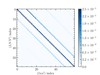
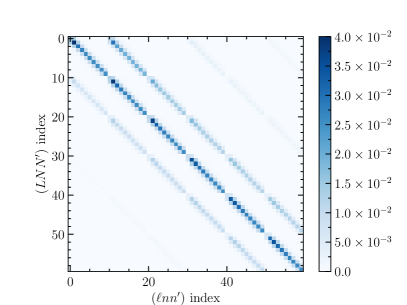
Figure 2: In the left panel we show the mixing matrix $\mathcal{M}_{\ell nn^{\prime}}^{LNN^{\prime}}$ for a half-sky mask, and in the right panel we add a radial selection function. The ordering of the $(\ell nn^{\prime})$ modes is such that $n=n^{\prime}$ increases first from 1 to 10, and $\ell$ increases by one for every ten $n$-modes. The half-sky mask in the left panel exhibits couplings between neighboring $\ell$-modes. On the right, the radial selection function decreases with distance, which leads to neighboring $n$-modes being coupled as well.

It is quite common that the window function is separable into a radial and an angular term,

$$W({\bm{r}}) =\phi(r)\,M({\hat{\bm{r}}})\,.$$ (53)

If the flux limit in a blind survey is near $L^{*}$, then the selection could change dramatically as a function of angular depth variations that are due to, e.g., atmospheric variations, and the separation of angular and radial selection would be a poor approximation. However, eBOSS, for example, had more targets selected in regions where two or more plates overlapped (e.g. de Mattia et al., 2021). Similarly, PFS will have higher target numbers where pointings overlap (Sunayama et al., 2020).

When the window function is separable, then Eq. 39 is separable as well,

$$W_{LM}(r) =\phi(r)\,W_{LM}\,,$$ (54)

where

$$W_{LM} =\int\mathrm{d}^{2}{\hat{\bm{r}}}\,Y^{*}_{LM}({\hat{\bm{r}}})\,M({\hat{\bm{r}}})\,,$$ (55)

and Eq. 52 becomes

$$\mathcal{M}_{\ell nn^{\prime}}^{LNN^{\prime}} =\frac{2L+1}{4\pi}\sum_{L_{1}}\begin{pmatrix}\ell&L&L_{1}\\ 0&0&0\end{pmatrix}^{2}\sum_{M_{1}}\left|W_{L_{1}M_{1}}\right|^{2}$$

$$\quad\times\int\mathrm{d}r\,r^{2}\,g_{n\ell}(r)\,g_{NL}(r)\,\phi(r)$$

$$\quad\times\int\mathrm{d}r^{\prime}\,r^{\prime 2}\,g_{n^{\prime}\ell}(r^{\prime})\,g_{N^{\prime}L}(r^{\prime})\,\phi(r^{\prime})\,,$$ (56)

which is also separable, and therefore significantly reduces computation cost. Eq. 40 simplifies in a similar manner.

In the special case that $W({\bm{r}})=1$ everywhere, we recover the unit matrix

$$\mathcal{M}_{\ell nn^{\prime}}^{LNN^{\prime}} =\delta^{K}_{\ell L}\delta^{K}_{nN}\delta^{K}_{n^{\prime}N^{\prime}}\,,$$ (57)

as expected.

We give two further examples in Fig. 2. In the left panel, we show the mixing matrix for a mask covering half the sky, and this leads to coupling of neighboring $\ell$-modes. On the right, we add a radial selection decreasing with redshift, and this additionally leads to the coupling of neighboring $n$-modes.

III.5 Shot noise

The sampling of the density field by a limited number of points leads to a shot noise component in the power spectrum. To estimate the shot noise, we start with (Peebles, 1973; Feldman et al., 1994)

$$\left\langle n({\bm{r}})\,n({\bm{r}}^{\prime})\right\rangle =\bar{n}({\bm{r}})\,\bar{n}({\bm{r}}^{\prime})\left[1+\xi({\bm{r}},{\bm{r}}^{\prime})\right]$$

$$\quad+\bar{n}({\bm{r}})\,\delta^{D}({\bm{r}}-{\bm{r}}^{\prime})\,,$$ (58)

$$\left\langle n({\bm{r}})\,n_{r}({\bm{r}}^{\prime})\right\rangle =\alpha^{-1}\,\bar{n}({\bm{r}})\,\bar{n}({\bm{r}}^{\prime})\,,$$ (59)

$$\left\langle n_{r}({\bm{r}})\,n_{r}({\bm{r}}^{\prime})\right\rangle =\alpha^{-2}\,\bar{n}({\bm{r}})\,\bar{n}({\bm{r}}^{\prime})+\alpha^{-1}\,\bar{n}({\bm{r}})\,\delta^{D}({\bm{r}}-{\bm{r}}^{\prime})\,.$$ (60)

The density contrast is given by Eq. 32, and the ensemble average becomes

$$\left\langle\delta^{\mathrm{obs}}({\bm{r}})\,\delta^{\mathrm{obs}}({\bm{r}}^{\prime})\right\rangle =W({\bm{r}})\,W({\bm{r}}^{\prime})\,\xi({\bm{r}},{\bm{r}}^{\prime})$$

$$\quad+(1+\alpha)\,\frac{W({\bm{r}})\,\delta^{D}({\bm{r}}^{\prime}-{\bm{r}})}{\bar{n}}\,,$$ (61)

where we used Eq. 29. Therefore, the SFB transform of the shot noise term becomes (see Eq. 28)

$$N^{\mathrm{obs}} =\frac{1}{\bar{n}}\,\mathrm{SFB}^{2}[W({\bm{r}})\delta^{D}({\bm{r}}^{\prime}-{\bm{r}})]$$ (62)

$$=\frac{1}{\bar{n}}\,W_{n\ell m}^{n^{\prime}\ell^{\prime}m^{\prime}}\,,$$ (63)

in the limit $\alpha\to 0$, and the $W$ matrix is defined in Section III.2. The window-corrected shot noise, therefore, is, in matrix form, $W^{-1}/\bar{n}$.

For the pseudo-SFB-power-spectrum estimator the shot noise simplifies significantly. Averaging over the modes $m=m^{\prime}$ and assuming $\ell=\ell^{\prime}$, Eq. 63 becomes

$$N_{\ell nn^{\prime}}^{\mathrm{obs}} =\frac{1}{{\bar{n}}}\,\frac{1}{\sqrt{4\pi}}\,\int\mathrm{d}r\,r^{2}\,g_{n\ell}(r)\,g_{n^{\prime}\ell}(r)\,W_{00}(r)\,,$$ (64)

where we used Eq. 40. Eq. 64 can be implemented very efficiently.

III.6 Pixel window

The pixel window refers to a distortion of the power spectrum due to binning galaxies into pixels. In the radial direction, we do not bin the galaxies, see Eq. 44, and, therefore, we do not have a radial pixel window (Leistedt et al., 2012).

However, the signal in Eq. 49 is still affected by the pixel window from the spherical harmonic transform. We correct this by subtracting the shot noise from the observed power spectrum, then using the pixwin function of HealPy to correct for the pixel window. We confirm the accuracy of this procedure with simulations in Section IV.

III.7 Bandpowers

We use a similar approach as Hivon et al. (2002); Alonso et al. (2019) to bin the SFB power spectrum into bandpowers. This is necessary if one wants to estimate the SFB power spectrum itself, as the mixing matrices in Sections III.2 and 50 are, in general, not invertible with finite-precision arithmetic. Compared to those authors our situation is complicated, but not significantly changed, by the fact that we may need to bin not only in $\ell$, but also in the $k$-modes $n$ and $n^{\prime}$.

We define the bandpower-binned pseudo-$C_{\ell}$ SFB power spectrum as a weighted sum over modes,

$$\hat{B}^{\mathrm{obs}}_{LNN^{\prime}} =\sum_{\ell nn^{\prime}}\widetilde{w}_{LNN^{\prime}}^{\ell nn^{\prime}}\,\hat{C}^{\mathrm{obs}}_{\ell nn^{\prime}}\,,$$ (65)

where $\widetilde{w}_{LNN^{\prime}}^{\ell nn^{\prime}}$ is typically a rectangular sparse matrix that takes the average of neighboring modes $(\ell nn^{\prime})\sim(LNN^{\prime})$. The operation Eq. 65 is a type of compression, where the compression matrix $\widetilde{w}$ must satisfy the normalization

$$\sum_{\ell nn^{\prime}}\widetilde{w}_{LNN^{\prime}}^{\ell nn^{\prime}} =1\,.$$ (66)

In matrix notation, we write the compression operation Eq. 65 and the corresponding decompression operation

$$B^{W} =\widetilde{w}C^{W}\,, C^{W} \simeq\widetilde{v}B^{W}\,,$$ (67)

$$B =wC\,, C \simeq vB\,,$$ (68)

where $\widetilde{w}$ and $\widetilde{v}$ are rectangular matrices operating on window-convolved power spectra, and $w$ and $v$ are rectangular matrices operating on cleaned power spectra. We use the index ‘W’ to indicate that we are only considering the window convolution. That is,

$$C^{W} =\mathcal{M}C\,, B^{W} =\mathcal{N}B\,,$$ (69)

where $\mathcal{M}$ is given by Eq. 51, and we can use the first of Eq. 67, the first of Eq. 69, and the last of Eq. 68 to get

$$\mathcal{N} =\widetilde{w}\mathcal{M}v\,.$$ (70)

The compression matrix $w$ is obtained by inverting the second of Eq. 69, using the first of Eq. 67, and the first of Eq. 69 to get

$$B =\mathcal{N}^{-1}B^{W}=\mathcal{N}^{-1}\widetilde{w}C^{W}=\mathcal{N}^{-1}\widetilde{w}\mathcal{M}C\,,$$ (71)

or (Alonso et al., 2019),

$$w =\mathcal{N}^{-1}\widetilde{w}\mathcal{M}\,.$$ (72)

Similarly, we find

$$\widetilde{v} =\mathcal{M}v\mathcal{N}^{-1}\,.$$ (73)

Eq. 70 then implies that

$$wv=\widetilde{w}\,\widetilde{v} =I\,.$$ (74)

Eq. 74 is equivalent to assuming that a decompression-then-recompression cycle is lossless. That is, the compressed representation is unaffected by decompression. The opposite, compression-then-decompression, however, will in general incur losses in the compression step, so that $vw\neq I$ except in special cases.

Furthermore, once the information is lost, repeated compression-then-decompression cycles do not lose more information. That is, $(vw)^{n}=vw$ for integer $n\geq 1$.

Note that $w$ and $\widetilde{v}$ must be calculated via Eqs. 72 and 73, because in the general case we have $(vw)^{\dagger}\neq vw$, and, therefore, they are not unique in satisfying Eq. 74. That is, they are not the unique Moore-Penrose inverses of the matrices $v$ and $\widetilde{w}$ (Dresden, 1920; Penrose, 1955).

Since $w$ and $\widetilde{v}$ can be expressed in terms of $\widetilde{w}$, $v$, and the window mixing matrix, our procedure consists of choosing a compression matrix $\widetilde{w}$ and a decompression matrix $v$.

How to choose $\widetilde{w}$ and $v$? For $\widetilde{w}$ we have already suggested that its operation on a power spectrum shall weigh neighboring modes equally and satisfy the normalization Eq. 66. Since the modes $n$ and $n^{\prime}$ refer to modes $k_{n\ell}$, their spacing is not independent, and we need to bin four modes, nine modes, or similar at a time. In this paper, our binning strategy is completely specified by the two numbers $\Delta\ell$ and $\Delta n$.

A natural choice for the decompression $v$ is, then, as the Moore-Penrose inverse of $\widetilde{w}$. Indeed, for the aforementioned choice for $\widetilde{w}$ that takes the average of neighboring modes, this means that $v$ is a step function that assigns the same value or a value proportional to $\ell\left(\ell+1\right)$ to all modes within a bin (Hivon et al., 2002; Alonso et al., 2019).

Finally, to compare the binned power spectrum with a theoretical estimate the first of Eq. 68 must be applied to the theoretical prediction.

III.8 Local Average Effect

In this section we recognize that the average number density ${\bar{n}}$ in Eq. 32 must in practice be measured from the survey itself. This is often called the integral constraint (Beutler et al., 2014; de Mattia and Ruhlmann-Kleider, 2019) or the local average effect (de Putter et al., 2012; Wadekar et al., 2020), and here we show that it suppresses the largest measured SFB mode in the survey.

Measuring the average number density is accomplished by dividing the total number of galaxies in the survey by the effective volume. However, the total number of galaxies in the survey is a stochastic quantity such that the average number density is given by

$${\bar{n}} =\left(1+\bar{\delta}\,\right){\bar{n}}^{\mathrm{true}}\,,$$ (75)

where ${\bar{n}}^{\mathrm{true}}$ is the underlying density contrast in the whole universe, and the average density contrast in the survey volume is

$$\bar{\delta} =\frac{1}{V_{\mathrm{eff}}}\int\mathrm{d}^{3}{\bm{r}}\,W({\bm{r}})\,\delta({\bm{r}})\,,$$ (76)

with the effective volume defined in Eq. 30. Therefore, with our model in Eq. 32, the measured density contrast is (Taruya et al., 2021)

$$\delta^{\mathrm{obs}}({\bm{r}})\equiv\delta^{W,A}({\bm{r}}) =W({\bm{r}})\,\frac{\delta({\bm{r}})-\bar{\delta}}{1+\bar{\delta}}\,,$$ (77)

where $\delta({\bm{r}})$ is the true density contrast, the superscript ‘A’ refers to the local average effect, and the superscript ‘W’ refers to the effect of the window convolution.

The SFB transform of Eq. 77 is

$$\delta^{W,A}_{n\ell m} =\sum_{n^{\prime}\ell^{\prime}m^{\prime}}W_{n\ell m}^{n^{\prime}\ell^{\prime}m^{\prime}}\,\frac{\delta_{n^{\prime}\ell^{\prime}m^{\prime}}-d_{n^{\prime}\ell^{\prime}m^{\prime}}\,\bar{\delta}}{1+\bar{\delta}}\,,$$ (78)

where we used Eqs. 34 and 28, and we defined

$$d_{n^{\prime}\ell^{\prime}m^{\prime}} =\sqrt{4\pi}\,\delta^{K}_{\ell^{\prime}0}\delta^{K}_{m^{\prime}0}\int\mathrm{d}r\,r^{2}\,g_{n^{\prime}0}(r)\,.$$ (79)

Using Eqs. 34, 27 and 28, Eq. 76 can be written

$$\bar{\delta} =\frac{1}{V_{\mathrm{eff}}}\sum_{n^{\prime}\ell^{\prime}m^{\prime}}d^{W,*}_{n^{\prime}\ell^{\prime}m^{\prime}}\,\delta_{n^{\prime}\ell^{\prime}m^{\prime}}\,,$$ (80)

where we used Eq. 37 to define $d^{W}_{n^{\prime}\ell^{\prime}m^{\prime}}$ as

$$d^{W}_{n^{\prime}\ell^{\prime}m^{\prime}} =\sum_{n\ell m}W^{n\ell m}_{n^{\prime}\ell^{\prime}m^{\prime}}\,d_{n\ell m}\,.$$ (81)

Then, expanding Eq. 78 for small $\bar{\delta}$ we get

$$\delta^{W,A}_{n\ell m} =\sum_{n^{\prime}\ell^{\prime}m^{\prime}}W_{n\ell m}^{n^{\prime}\ell^{\prime}m^{\prime}}\Big{[}\delta_{n^{\prime}\ell^{\prime}m^{\prime}}-d_{n^{\prime}\ell^{\prime}m^{\prime}}\,\bar{\delta}-\delta_{n^{\prime}\ell^{\prime}m^{\prime}}\bar{\delta}$$

$$\qquad+d_{n^{\prime}\ell^{\prime}m^{\prime}}\,\bar{\delta}^{2}+\delta_{n^{\prime}\ell^{\prime}m^{\prime}}\bar{\delta}^{2}+\mathcal{O}(\bar{\delta}^{3})\Big{]}.$$ (82)

Since $d_{n\ell m}\sim\sqrt{V}$ and $\bar{\delta}\sim 1/\sqrt{V}$ we expand in the volume $V$. We also assume $C_{\ell nn^{\prime}}\ll V_{\mathrm{eff}}$. Then, the correlation function becomes

$$\left\langle\delta^{W,A}_{NLM}\,\delta^{W,A,*}_{N^{\prime}L^{\prime}M^{\prime}}\right\rangle$$

$$=\sum_{n\ell m}W_{NLM}^{n\ell m}\sum_{n^{\prime}\ell^{\prime}m^{\prime}}W_{N^{\prime}L^{\prime}M^{\prime}}^{n^{\prime}\ell^{\prime}m^{\prime},*}$$

$$\quad\times\Big{[}\left\langle\delta_{n\ell m}\,\delta^{*}_{n^{\prime}\ell^{\prime}m^{\prime}}\right\rangle-\left\langle\delta_{n\ell m}\,\bar{\delta}\right\rangle d_{n^{\prime}\ell^{\prime}m^{\prime}}-d_{n\ell m}\left\langle\delta^{*}_{n^{\prime}\ell^{\prime}m^{\prime}}\,\bar{\delta}\right\rangle$$

$$\qquad+d_{n\ell m}d_{n^{\prime}\ell^{\prime}m^{\prime}}\left\langle\bar{\delta}^{2}\right\rangle+\mathcal{O}\!\left(V^{-\frac{1}{2}}\right)\Big{]},$$ (83)

where we assume the field $\delta$ to be Gaussian. The 2-point terms entering this expression are

$$\left\langle\delta_{n\ell m}\,\delta^{*}_{n^{\prime}\ell^{\prime}m^{\prime}}\right\rangle =\delta^{K}_{\ell\ell^{\prime}}\delta^{K}_{mm^{\prime}}\,C_{\ell nn^{\prime}}+\frac{1}{{\bar{n}}}\,(W^{-1})_{n\ell m}^{n^{\prime}\ell^{\prime}m^{\prime}}\,,$$ (84)

$$\left\langle\delta_{n\ell m}\,\bar{\delta}\right\rangle =\frac{1}{V_{\mathrm{eff}}}\sum_{n^{\prime\prime}}d^{W}_{n^{\prime\prime}\ell m}\,C_{\ell nn^{\prime\prime}}+\frac{1}{{\bar{n}}V_{\mathrm{eff}}}\,d_{n\ell m}\,,$$ (85)

$$\left\langle\bar{\delta}^{2}\right\rangle =\frac{1}{V^{2}_{\mathrm{eff}}}\sum_{\ell_{1}n_{1}n_{2}}D^{W}_{\ell_{1}n_{1}n_{2}}\,C_{\ell_{1}n_{1}n_{2}}$$

$$\quad+\frac{1}{{\bar{n}}V^{2}_{\mathrm{eff}}}\sum_{n_{1}\ell_{1}m_{1}}\,d_{n_{1}\ell_{1}m_{1}}\,d^{W}_{n_{1}\ell_{1}m_{1}}\,,$$ (86)

where we included the shot noise term Eq. 63, and we defined the unnormalized power spectrum of a constant field

$$D^{W}_{\ell_{1}n_{1}n_{2}} =\sum_{m_{1}}d^{W}_{n_{1}\ell_{1}m_{1}}\,d^{W,*}_{n_{2}\ell_{1}m_{1}}$$ (87)

$$=\left(2\ell_{1}+1\right)\sum_{n^{\prime}_{1}}\sum_{n^{\prime}_{2}}\mathcal{M}^{0n^{\prime}_{1}n^{\prime}_{2}}_{\ell_{1}n_{1}n_{2}}\,d_{n^{\prime}_{1}00}\,d_{n^{\prime}_{2}00}\,,$$ (88)

and Eq. 51 was used in the last line. Now the correlation function becomes

$$\left\langle\delta^{A}_{n\ell m}\,\delta^{A,*}_{n^{\prime}\ell^{\prime}m^{\prime}}\right\rangle =\delta^{K}_{\ell\ell^{\prime}}\delta^{K}_{mm^{\prime}}\,C_{\ell nn^{\prime}}+\frac{1}{{\bar{n}}}\,(W^{-1})_{n\ell m}^{n^{\prime}\ell^{\prime}m^{\prime}}-d_{n^{\prime}\ell^{\prime}m^{\prime}}\frac{1}{V_{\mathrm{eff}}}\sum_{n^{\prime\prime}}d^{W}_{n^{\prime\prime}\ell m}\,C_{\ell nn^{\prime\prime}}-d_{n\ell m}\frac{1}{V_{\mathrm{eff}}}\sum_{n^{\prime\prime}}d^{W,*}_{n^{\prime\prime}\ell^{\prime}m^{\prime}}\,C_{\ell^{\prime}n^{\prime}n^{\prime\prime}}$$

$$\quad+\left[\frac{-2}{{\bar{n}}V_{\mathrm{eff}}}+\left\langle\bar{\delta}^{2}\right\rangle\right]\,d_{n\ell m}\,d_{n^{\prime}\ell^{\prime}m^{\prime}}+\mathcal{O}\!\left(V^{-\frac{1}{2}}\right),$$ (89)

where we corrected for the window function. Only the first and fifth terms are proportional to $\delta^{K}_{\ell\ell^{\prime}}\delta^{K}_{mm^{\prime}}$, and so we cannot take the pseudo-$C_{\ell nn^{\prime}}$ power spectrum at this stage. To do so, we now add back the two window functions in Section III.8 to get a prediction for the observed pseudo power spectrum

$$C^{W,A}_{LNN^{\prime}} =\sum_{\ell nn^{\prime}}\mathcal{M}^{\ell nn^{\prime}}_{LNN^{\prime}}\,C_{\ell nn^{\prime}}+N^{\mathrm{obs}}_{LNN^{\prime}}-\frac{1}{V_{\mathrm{eff}}}\,\frac{1}{2L+1}\sum_{M}d^{W,*}_{N^{\prime}LM}\sum_{n\ell m}W_{NLM}^{n\ell m}\sum_{n^{\prime\prime}}d^{W}_{n^{\prime\prime}\ell m}\,C_{\ell nn^{\prime\prime}}$$

$$\quad-\frac{1}{V_{\mathrm{eff}}}\,\frac{1}{2L+1}\sum_{M}d^{W}_{NLM}\sum_{n^{\prime}\ell^{\prime}m^{\prime}}W_{N^{\prime}LM}^{n^{\prime}\ell^{\prime}m^{\prime},*}\sum_{n^{\prime\prime}}d^{W,*}_{n^{\prime\prime}\ell^{\prime}m^{\prime}}\,C_{\ell^{\prime}n^{\prime}n^{\prime\prime}}+\sum_{\ell nn^{\prime}}\mathcal{M}_{LNN^{\prime}}^{\ell nn^{\prime}}\,\delta^{K}_{\ell 0}d_{n00}d_{n^{\prime}00}\left[\frac{-2}{{\bar{n}}V_{\mathrm{eff}}}+\left\langle\bar{\delta}^{2}\right\rangle\right]$$

$$\quad+\mathcal{O}\!\left(V^{-\frac{1}{2}}\right),$$ (90)

where we used Eq. 64. The third and fourth terms are the same except for $N\leftrightarrow N^{\prime}$. To simplify these two terms, we express them in terms of chains of window functions $W_{k}$ that we define in Eq. 191 and study in Appendix F. We use Eq. 81 and get

$$\sum_{M}d^{W,*}_{N^{\prime}LM}\sum_{n\ell m}W_{NLM}^{n\ell m}\sum_{n^{\prime\prime}}d^{W}_{n^{\prime\prime}\ell m}\,C_{\ell nn^{\prime\prime}} =\sum_{M}\sum_{n^{\prime}\ell^{\prime}m^{\prime}}\sum_{n\ell m}\sum_{n^{\prime\prime}}\sum_{n_{1}\ell_{1}m_{1}}W_{N^{\prime}LM}^{n^{\prime}\ell^{\prime}m^{\prime},*}W_{NLM}^{n\ell m}W_{n^{\prime\prime}\ell m}^{n_{1}\ell_{1}m_{1}}\,d_{n^{\prime}\ell^{\prime}m^{\prime}}\,d_{n_{1}\ell_{1}m_{1}}\,C_{\ell nn^{\prime\prime}}$$

$$=\sum_{\ell nn^{\prime\prime}}\sum_{\ell^{\prime}n_{1}n^{\prime}}\sum_{Mmm^{\prime}}W^{N^{\prime}LM}_{n^{\prime}\ell^{\prime}m^{\prime}}W_{NLM}^{n\ell m}W_{n^{\prime\prime}\ell m}^{n_{1}\ell^{\prime}m^{\prime}}\,\delta^{K}_{\ell^{\prime}0}\,d_{n^{\prime}00}\,d_{n_{1}00}\,C_{\ell nn^{\prime\prime}}$$

$$=\sum_{\ell^{\prime}n_{1}n^{\prime}}\delta^{K}_{\ell^{\prime}0}\,d_{n^{\prime}00}\,d_{n_{1}00}\sum_{\ell nn^{\prime\prime}}C_{\ell nn^{\prime\prime}}\,W_{3}\!\!\begin{pmatrix}L&\ell&\ell^{\prime}\\ N^{\prime}&n&n_{1}\\ N&n^{\prime\prime}&n^{\prime}\end{pmatrix},$$ (91)

where $W_{3}$ is defined in Eq. 191. Section III.8 now becomes

$$C^{W,A}_{LNN^{\prime}} =\sum_{\ell nn^{\prime}}\mathcal{M}^{\ell nn^{\prime}}_{LNN^{\prime}}\left[C_{\ell nn^{\prime}}+\delta^{K}_{\ell 0}d_{n00}d_{n^{\prime}00}\left(\frac{-2}{{\bar{n}}V_{\mathrm{eff}}}+\left\langle\bar{\delta}^{2}\right\rangle\right)\right]+N^{\mathrm{obs}}_{LNN^{\prime}}$$

$$\quad-\frac{1}{V_{\mathrm{eff}}}\,\frac{1}{2L+1}\sum_{\ell^{\prime}n_{1}n^{\prime}}\delta^{K}_{\ell^{\prime}0}\,d_{n_{1}00}\,d_{n^{\prime}00}\sum_{\ell nn^{\prime\prime}}C_{\ell nn^{\prime\prime}}\left[W_{3}\!\!\begin{pmatrix}L&\ell&\ell^{\prime}\\ N^{\prime}&n&n_{1}\\ N&n^{\prime\prime}&n^{\prime}\end{pmatrix}+\left\langle N\leftrightarrow N^{\prime}\right\rangle\right].$$ (92)

The window de-convolved power spectrum is then $C^{A}=\mathcal{M}^{-1}C^{W,A}$.

In the absence of a window function and assuming $C_{\ell nn^{\prime}}\,\propto\,\delta^{K}_{nn^{\prime}}$, as well as using Eq. 79, we get

$$C^{A}_{\ell nn^{\prime}} \simeq\left(1+\frac{3A\,C_{011}}{V_{\mathrm{eff}}}\right)C_{\ell nn^{\prime}}-\delta^{K}_{\ell 0}\,\frac{d_{n00}\,d_{n^{\prime}00}}{V_{\mathrm{eff}}}\,B_{nn^{\prime}}\,,$$ (93)

where we included further terms from the expansion Section III.8, and we defined

$$A =\sum_{n_{1}}\frac{d_{n_{1}00}^{2}}{V_{\mathrm{eff}}}\,\frac{C_{0n_{1}n_{1}}}{C_{011}}\,,$$ (94)

$$B_{nn^{\prime}} =C_{0nn}+C_{0n^{\prime}n^{\prime}}-A\,C_{011}-\frac{6\,C_{0nn}\,C_{0n^{\prime}n^{\prime}}}{V_{\mathrm{eff}}}\,.$$ (95)

To a good approximation $A\simeq 1$, and the last term in $B_{nn^{\prime}}$ can be neglected if the effective volume is sufficiently large and the shot noise sufficiently low. Furthermore, a good approximation is $d_{n00}\,\propto\,\delta^{K}_{n1}$. Therefore, only the $(\ell,n,n^{\prime})=(0,1,1)$ mode is significantly affected. That is, the main effect of super-sample variance on the measured power spectrum is to reduce the power in the largest mode.

III.9 Covariance matrix of power spectrum

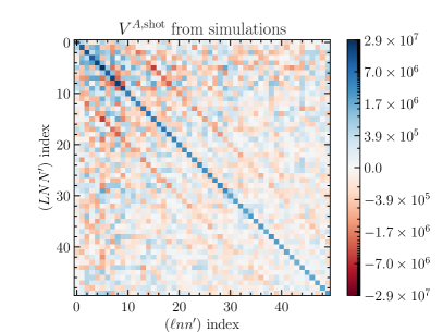
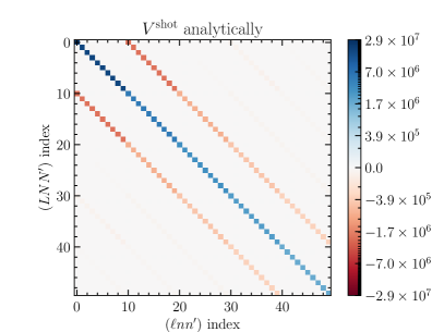
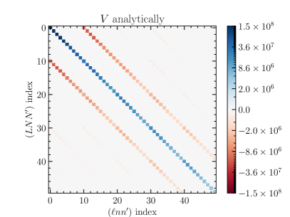
Figure 3: The panels show the covariance matrix $V$ defined in Eq. 97. Top row: $V^{A}$ as measured from 100 simulations, including the local average effect. Bottom row: The analytical prediction, without local average effect. Left column: Shot noise only. Right column: Linear power spectrum with shot noise. Here we use a simulation with $50\text{\,}\mathrm{\char 37\relax}$ sky coverage and bandpower binning with $\Delta\ell=2$. The order of the $(\ell nn^{\prime})$ indices is such that each block of ten indices is for one $\ell$-bin starting with $\ell=0,1$ for the block starting with index 0 and ending with $\ell=8,9$ for the block starting at index 40. Within each block $n=n^{\prime}$ increases from one to 10. Note that the nonlinear color scheme amplifies small elements.

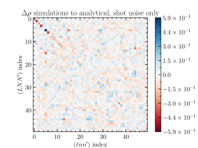
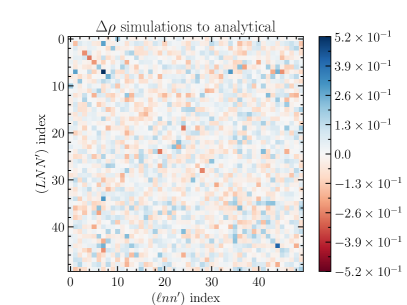
Figure 4: Relative comparison between the covariance matrices as in Eq. 101. This avoids amplifying small deviations far from the center diagonal, and it shows that the analytic result largely agrees with the simulations. The very largest mode is set to zero, because it is affected by the local average effect that is not included in the analytical result (see Fig. 5).

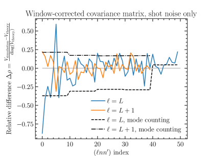
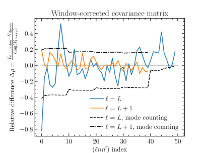
Figure 5: Comparison of the diagonal and the $\ell=L+1$ off-diagonal window-corrected covariance between simulations and analytical result. Left shows the shot noise only, and right including shot noise and a non-zero power spectrum. In the analytical result we do not include local average effect. Thus, the first mode in the simulations is suppressed compared to the analytical result. The black dashed and dash-dotted lines show the approximate result from mode-counting Eq. 98.

In this section we provide a covariance matrix for the SFB power spectrum. Several approaches have been used previously. Percival et al. (2004); Wang et al. (2020) trace the likelihood function either on a grid or using Markov Chain Monte Carlo techniques. Wang et al. (2020), e.g., use simulations to measure the covariance matrix from suites of mock catalogues. An analytical approach for the 3D power spectrum multipoles is presented in Wadekar and Scoccimarro (2020). In this paper, we get an analytical estimate for the SFB power spectrum assuming that the density contrast is Gaussian, and we compare to 100 log-normal simulations. Non-Gaussian terms in the form of the disconnected trispectrum could be included similarly to Taruya et al. (2021); Sugiyama et al. (2020).

Super-sample variance (e.g., de Putter et al., 2012; Lacasa and Grain, 2019; Li et al., 2018) can have a significant impact on the covariance matrix. Beat coupling is mode mixing due to the window function with correlation between pairs of non-linear modes and one large mode. The local average effect is due to the large-scale mode modulating the average number density inside the survey volume. Both these effects can be treated in the manner of Sections III.8 and 77.

The covariance matrix on the observed SFB power spectrum is

$$V_{\ell nn^{\prime}}^{LNN^{\prime},\mathrm{obs}}\equiv\left\langle\hat{C}^{\mathrm{obs}}_{\ell nn^{\prime}}\,\hat{C}^{\mathrm{obs}}_{LNN^{\prime}}\right\rangle-C^{\mathrm{obs}}_{\ell nn^{\prime}}\,C^{\mathrm{obs}}_{LNN^{\prime}}$$

$$=\frac{1}{(2\ell+1)(2L+1)}\sum_{mM}\Big{[}\left\langle\delta^{W,A}_{n\ell m}\delta^{W,A}_{NLM}\right\rangle\left\langle\delta^{{W,A},*}_{n^{\prime}\ell m}\delta^{{W,A},*}_{N^{\prime}LM}\right\rangle$$

$$\quad+\left\langle\delta^{W,A}_{n\ell m}\delta^{{W,A},*}_{N^{\prime}LM}\right\rangle\left\langle\delta^{W,A}_{NLM}\delta^{{W,A},*}_{n^{\prime}\ell m}\right\rangle\Big{]},$$ (96)

where we used Wick’s theorem for a Gaussian density contrast. We simplify Section III.9 in Appendix E. However, an analytical calculation remains computationally expensive.

To get the covariance matrix for the window-corrected power spectrum, we write the matrix equation

$$V =\mathcal{N}^{-1}\,V^{\mathrm{obs}}\,\mathcal{N}^{-1,T}\,.$$ (97)

where $\mathcal{N}$ is the bandpower-binned window coupling matrix given in Eq. 70, and the binning of the covariance matrix is implied.

A reasonably precise estimate can be obtained by counting modes and assuming the covariance matrix is diagonal. That is,

$$V_{\ell nn^{\prime}}^{LNN^{\prime}} \simeq\frac{\delta^{K}_{\ell L}}{N_{\mathrm{modes}}}\left[C_{\ell nN}^{\mathrm{binned}}C_{Ln^{\prime}N^{\prime}}^{\mathrm{binned}}+C_{\ell nN^{\prime}}^{\mathrm{binned}}C_{Ln^{\prime}N}^{\mathrm{binned}}\right],$$ (98)

where the power spectrum includes the shot noise, $C_{\ell nn^{\prime}}^{\mathrm{binned}}=C^{\mathrm{signal}}_{\ell nn^{\prime}}+N^{\mathrm{shot}}_{\ell nn^{\prime}}$, and

$$N_{\mathrm{modes}} =f_{\mathrm{vol}}\,(2\ell+1)\,\Delta\ell\,\Delta n\,,$$ (99)

where $\Delta\ell$ and $\Delta n$ are the bin widths for modes $k_{n\ell}$, and $f_{\mathrm{vol}}$ is the fraction of the SFB transform-volume that is occupied by the survey, defined by

$$f_{\mathrm{vol}} \equiv\frac{1}{V_{\mathrm{SFB}}}\int\mathrm{d}^{3}{\bm{r}}\,\tau\!\left[W({\bm{r}})-W_{\mathrm{threshold}}\right],$$ (100)

where $\tau(x)$ is a step function and $W_{\mathrm{threshold}}$ is a threshold of the window function.

The shot noise takes into account the variation of the number density across the survey, and it enters in Eq. 98 as part of the power spectrum. The incomplete volume coverage enters as a reduction in the number of modes, and it is needed for the stability of the window-deconvolution when there are large unobserved regions in the SFB volume.

In Fig. 3 we show the covariance matrices for a set of simulations that contain only shot noise (top left) as well as for a set of simulations with a physical galaxy power spectrum with bias $b=1.5$ at effective redshift $z_{\mathrm{eff}}=2$ (top right). In the figure we also show the analytical result from Section III.9 (bottom panels).

The colorbar in the figure is nonlinear. As a result, small elements appear amplified. To provide a more useful comparison, we introduce the difference between two covariance matrices, scaled to the center diagonal. That is, we introduce the relative difference

$$\Delta\rho_{ij} =\frac{C^{A}_{ij}-C^{B}_{ij}}{\sqrt{C^{B}_{ii}\,C^{B}_{jj}}}\,,$$ (101)

and we choose $C^{B}$ to refer to the analytic result. $\Delta\rho$ does not suffer from amplification of small differences far from the diagonal.

Therefore, in Fig. 4 we show the relative difference between the covariance matrix as obtained from simulations and the analytical result. However, in the figure we remove the largest mode, since we have not included the local average effect in the analytical calculation. All other modes are statistically essentially equal between simulation result and analytics.

To show this more clearly, we present Fig. 5, where we compare the main diagonal and the $\ell=L+1$ diagonal of the covariance matrices using the same statistic Eq. 101. Within the noise, we find good agreement between simulations and analytical result.

III.10 Performance scaling

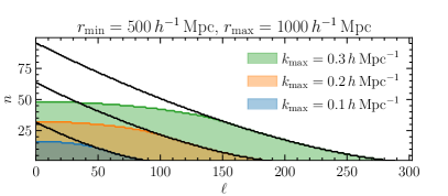
Figure 6: Here we show the modes that are required to achieve a given $k_{\mathrm{max}}$ for the given radial boundaries. The solid black curves are constant-$k$ contours for $r_{\mathrm{min}}=0$.

In this section we give a brief overview of the performance behavior of the code. We consider the scaling of the SFB decomposition, the coupling matrix, and the number of modes with the parameters of the SFB power spectrum estimation.

Typically, it is desirable to calculate all modes up to some $k_{\mathrm{max}}$. The total number of modes can be estimated in the same way as for a standard Fourier transform by estimating the fundamental frequency from the volume that is being transformed, i.e., $V_{\mathrm{SFB}}\simeq\frac{4\pi}{3}\left(r_{\mathrm{max}}^{3}-r_{\mathrm{min}}^{3}\right)$ and $k_{F}\simeq 2\pi/V_{\mathrm{SFB}}^{1/3}$. Then, the total number of modes is approximately $N_{\mathrm{modes}}\simeq\frac{4\pi}{3}\,k_{\mathrm{max}}^{3}/k_{F}^{3}\simeq\frac{1}{18\pi}\,k_{\mathrm{max}}^{3}\left(r_{\mathrm{max}}^{3}-r_{\mathrm{min}}^{3}\right)$. These are the modes that need to be calculated for transform.

However, as shown in Fig. 6, the boundary at $r_{\mathrm{min}}$ changes the structure about which modes need to be calculated. In the figure, modes with $k\leq k_{\mathrm{max}}$ are in the shaded region when, for illustration, $r_{\mathrm{min}}=$500\text{\,}{\mathrm{\text{$h$}}}^{-1}\text{\,}\mathrm{Mpc}$$, and all the modes below the solid black curves need to be calculated if $r_{\mathrm{min}}=0$. The figure shows that fewer low-$\ell$ modes are needed when $r_{\mathrm{min}}$ is finite. However, most modes are at large $\ell$, and, therefore, this is only a small computational reduction.

The algorithm now scales as follows. First, the sum in Eq. 44 is performed, and then for each $(n,\ell)$-combination the spherical harmonic transform Eq. 48 is performed. Hence, the execution time of the transform scales as

$$T \sim\mathcal{O}\!\left[n_{\mathrm{max}}\,\ell_{\mathrm{max}}\left(N_{\mathrm{gal}}+N^{\mathrm{Healpix}}_{\ell}\right)\right],$$ (102)

where $N^{\mathrm{Healpix}}_{\ell}\sim N_{\mathrm{pix}}^{3/2}$ is the number of operations needed for the spherical harmonic transform, and $N_{\mathrm{pix}}$ is the number of HEALPix pixels.

To estimate $N_{\mathrm{pix}}=12n_{\mathrm{side}}^{2}$, we need to estimate $n_{\mathrm{side}}$, which we do by considering the angular resolution. Recommended is $\ell_{\mathrm{max}}\simeq 2n_{\mathrm{side}}$. However, our algorithms dealing with the window function will need to go to $L=2\ell_{\mathrm{max}}$. Hence, we estimate

$$n_{\mathrm{side}} =2^{\mathrm{ceil}\left(\log_{2}\left(\ell_{\mathrm{max}}+\frac{1}{2}\right)\right)},$$ (103)

where $\mathrm{ceil}(x)$ is the smallest integer greater than $x$. Eq. 103 guarantees that $n_{\mathrm{side}}$ is a power of two.

The angular resolution is determined by $\ell_{\mathrm{max}}$, which is determined by $k_{\mathrm{max}}$ and $r_{\mathrm{max}}$ by Limber’s relation Eq. 149. However, we note that the actual number needed for $\ell_{\mathrm{max}}$ tends to be smaller by a few percent.

For the three surveys in Section IV below, the SFB analysis takes $\sim 10$ CPU-min per simulation for the Roman- and SPHEREx-like surveys, and $\sim 1.5$ CPU-hour for the Euclid-like survey. Calculation of the mixing matrix $\mathcal{M}$ for the three surveys is on the order of a few CPU-minutes, exploiting the angular/radial split, and would take several CPU-hours without that split. At present, the analytical covariance matrix is only feasible for the largest scales.

IV Future Applications

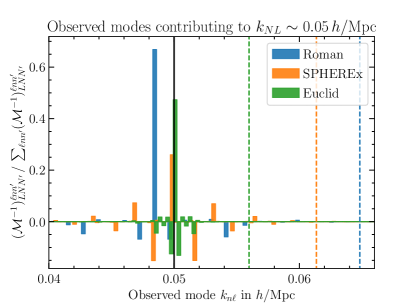
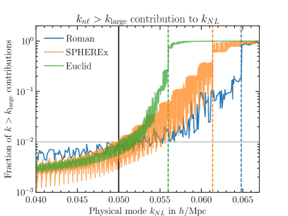
Figure 7: This figure shows the relative contributions from hi-$k$ observed (window-convolved) modes to physical modes close to $k_{\mathrm{max}}=$0.05\text{\,}\mathrm{\text{$h$}}\text{\,}{\mathrm{Mpc}}^{-1}$$ (vertical black line). The left panel shows a histogram of the contributions to a single physical mode. Since there are modes above $k_{\mathrm{max}}$ that are contributing in the deconvolution of the window (the inversion of Eq. 50) we include all the modes up to the dashed lines at $k_{\mathrm{large}}$, which are colored by survey. The specific physical mode chosen is the one that has the most contribution from modes above $k_{\mathrm{large}}$ (the dashed line), and the dashed lines are chosen so that their cumulative contribution is less than $1\text{\,}\mathrm{\char 37\relax}$. The right panel shows the cumulative contribution from observed modes $k>k_{\mathrm{large}}$ for each physical mode $k_{NL}$. The vertical lines are the same as in the left plot, the horizontal line marks our target maximum contribution of $1\text{\,}\mathrm{\char 37\relax}$.

In this section we will test the SFB estimator presented in this paper for several use cases. First, we will consider simplistic simulations of surveys similar to the High-Latitude Spectroscopic Survey (HLSS) of the Nancy Grace Roman Space Telescope which will benefit from large radial modes, and we will consider SPHEREx and Euclid for wide-angle surveys.

We bin into bandpowers by selecting

$$\Delta\ell \simeq\frac{1}{f_{\mathrm{sky}}}\,,$$ (104)

and then we round to the nearest integer. Eq. 99 then suggests

$$\Delta n \simeq\frac{f_{\mathrm{sky}}}{f_{\mathrm{vol}}}\,.$$ (105)

For all cases in this paper, this results in $\Delta n=1$.

To do the window deconvolution, it is important to ensure that all modes are complete. For the angular power spectrum, Leistedt et al. (2013); Alonso et al. (2019) suggest estimating up to $2\ell_{\mathrm{max}}$, and then discarding all the modes above $\ell_{\mathrm{max}}$. Wang et al. (2020) argue that (in our notation) the sum Eq. 50 only converges with the inclusion of modes $k_{n\ell}>k_{\mathrm{max}}$, and they do numerical experiments to estimate the maximum $k$ needed.

We take a similar approach, which is demonstrated in Fig. 7, where in the left panel the relative contribution of window-convolved modes to a physical mode near $k_{\mathrm{max}}$ is shown. That is, we plot the relative contributions of all observed modes $(\ell nn^{\prime})$ that contribute to the physical mode $(LNN^{\prime})$ using Eq. 50. Assuming a flat power spectrum and summing the absolute values of the coupling matrix $\mathcal{M}^{-1}$, then, allows us to estimate the contribution from all modes above some $k_{\mathrm{large}}$. This is shown in the right panel of Fig. 7.

Next, we iteratively increase $k_{\mathrm{large}}$ until the contribution from $k_{n\ell}>k_{\mathrm{large}}$ to the most affected mode $k_{NL}\leq{}k_{\mathrm{max}}$ is less than $1\text{\,}\mathrm{\char 37\relax}$. The results for $k_{\mathrm{large}}$ are the dashed vertical lines in either panel of Fig. 7.

That is, by including all modes up to $k_{\mathrm{large}}>k_{\mathrm{max}}$ in the SFB power spectrum estimation, we get reasonable confidence that all modes $k<k_{\mathrm{max}}$ can be fully deconvolved by the inversion of Eq. 50.

IV.1 Roman

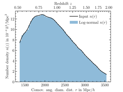
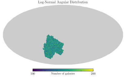
Figure 8: The plots show the approximate Roman radial selection function and angular mask. In addition one realization of a log-normal simulation is shown.

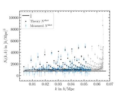
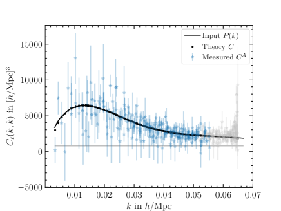
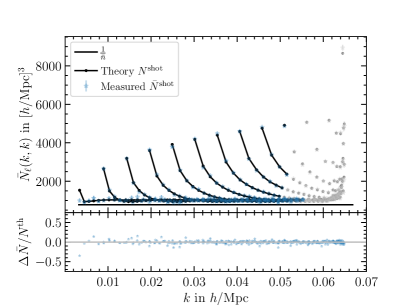
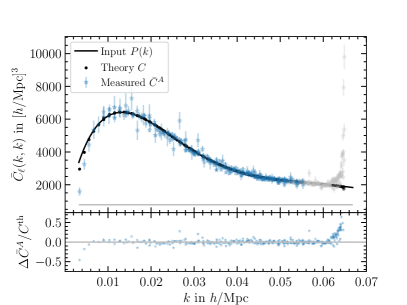
Figure 9: SFB power spectrum measurement from uniform shot-noise-only (left column) and log-normal (right column) simulations with Roman window function. The top row is for a single simulation, the bottom shows the average over 50 simulations, and in the top panels the error bars are for a single simulation, while in the bottom panels the error bars are divided by $\sqrt{50}$. In each panel, the grey-painted modes near $k_{\mathrm{max}}$ are incomplete bandpower bins, and we show them for illustration only. On the right panels, the theory points take into account the bandpower binning with $\Delta\ell=18$. The horizontal line in each plot is $\frac{1}{{\bar{n}}}$. The local average effect suppresses the largest-scale mode in the simulations. For better comparison between the average measured power spectrum and the theory points, we show the fractional difference of each mode at the bottom of the lower panels. Note that here we only consider an H$\alpha$ sample of Roman.

In this section we apply the SFB power spectrum estimator to a log-normal simulation for the High-Latitude Spectroscopy Survey (HLSS) of the Nancy Grace Roman Space Telescope (Spergel et al., 2015). The notional survey area is currently planned as $\sim 6\text{\,}\mathrm{\char 37\relax}$ of the sky. Our main objective here, however, is to exploit the large radial selection that Roman will provide.

The grism spectroscopy of the HLSS will yield observed wavelengths $1\text{\,}\mathrm{\SIUnitSymbolMicro m}1.93\text{\,}\mathrm{\SIUnitSymbolMicro m}$, which for the H$\alpha$ line at $6562.8\text{\,}\mathrm{\SIUnitSymbolAngstrom}$ results in a redshift range $0.523\leq z\leq 1.94$, and for the simulations we round this to the range $1370\text{\,}{\mathrm{\text{$h$}}}^{-1}\text{\,}\mathrm{Mpc}3540\text{\,}{\mathrm{\text{$h$}}}^{-1}\text{\,}\mathrm{Mpc}$. The radial selection for our simulation is shown in the left panel of Fig. 8 (Eifler et al., 2021).

The right panel of Fig. 8 shows the HEALPix projection of our log-normal simulation (Agrawal et al., 2017), where we use an approximate binary Roman mask. The window function is then constructed as the multiplication of the radial selection and mask, normalized so that the maximum is unity.

Our log-normal simulation assumes a non-evolving linear power spectrum at redshift 1.5 and linear galaxy bias $b=1.5$. The number of galaxies is $\sim 6.6\text{\times}{10}^{6}$. We use a flat $\Lambda$CDM Planck cosmology.

The results of the SFB analysis are shown in Fig. 9. The top left panel shows the shot noise from a simulation with vanishing power spectrum as well as the theoretical shot noise prediction from Eq. 64. The bottom left shows the average over 50 simulations.

For a simulation with signal, we show the SFB measurement from our log-normal simulation in the top right of Fig. 9. Here, we have subtracted the theoretical shot noise. The theory points and the input $P(k)$ differ due to application of Eq. 72 to account for the bandpower binning with $\Delta\ell=18$. The bottom right panel shows the same as an average over our ensemble of simulations.

We get good agreement between the ensemble measurement and theory power spectra if we restrict ourselves to the blue modes in Fig. 9. There are 213 modes with a $\chi^{2}_{\nu}=1.033$ in one simulation. The greyed-out modes cannot be fully deconvolved due to the possibility of high-$k$ contributions, as explained at the beginning of Section IV. Clearly, our estimations there were conservative, because high-$k$ contributions vary in sign and can cancel each other.

The black curves in the lower left panel of Fig. 9 connect theory points with the same $\ell$. For a given $\ell$, then, the limber ratio Eq. 149 suggests that higher $k$ corresponds to lower redshift. Since the number density tends to be higher at lower redshift, we expect the shot noise to decrease with $k$ given constant $\ell$. This effect is much more pronounced for SPHEREx below.

IV.2 SPHEREx

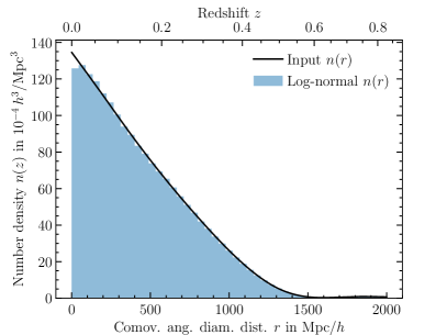
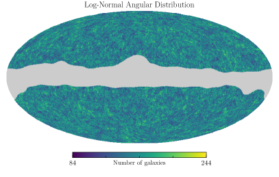
Figure 10: The plots show the approximate radial selection function and angular mask for our SPHEREx-like survey.

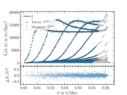
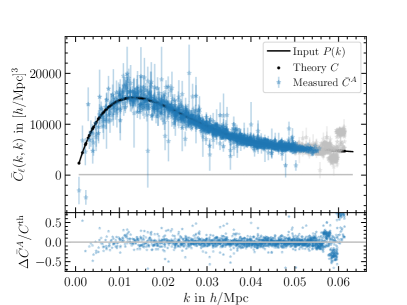
Figure 11: The plot on the left shows the shot noise and the plot on the right the SFB power spectrum similar to Fig. 9, but now for a full-sky mission like SPHEREx, averaged over 50 simulations with error bars divided by $\sqrt{50}$. Note that while the mask and selection are realistic, we only consider a small part of the full SPHEREx volume due to limitations of our mocks.

In this section we aim to show the feasibility of applying our estimator to SPHEREx (Doré et al., 2014).

For the radial selection, we use the SPHEREx public products, and for demonstration we limit ourselves to the range $0\leq r\leq$2000\text{\,}{\mathrm{\text{$h$}}}^{-1}\text{\,}\mathrm{Mpc}$$, corresponding to a maximum redshift of 0.83. We impose this limit due to our current lack of a large number of better simulations. The radial selection is shown in Fig. 10. SPHEREx is able to go down to essentially $z=0$ since it is not limited by the detection of a single emission line but measures galaxy redshifts with 102 narrow photometric bands.

For the mask we use the HFI GAL080 mask with no apodization from the Planck Collaboration. This cuts out the galactic plane, as shown in Fig. 10. The binning strategy in Eqs. 104 and 105 yields no binning, or $\Delta\ell=\Delta n=1$. The number of galaxies per simulation is $\sim 24$ million.

Since our log-normal simulations do not take into account redshift-evolution effects, we choose a fixed effective redshift $z_{\mathrm{eff}}=0.5$ and galaxy bias $b=1.5$.

The estimation of the SFB shot noise and power spectrum is shown in Fig. 11. The “dotted curves” of the theory shot noise that rise quickly and then settle on an approximately constant value are curves of constant $n$, and each dot along a curve signifies the increase of $\ell$ by one. That is, lines of constant $\ell$ start on the first of these curves, and then decrease rapidly, as expected from the Limber ratio Eq. 149 in conjuction with a high number density at low redshifts.

Fig. 11 shows that we get good agreement between our measured SFB power spectrum with the theory power spectrum. There are 1345 modes with a $\chi^{2}_{\nu}=1.020$ in one simulation. It is only in the greyed-out modes that are not fully deconvolved that a spurious oscillatory pattern is introduced, and measuring those modes accurately is simply a matter of increasing $k_{\mathrm{large}}$.

Furthermore, since in this paper we are primarily interested in testing the SFB estimator, Fig. 11 shows every mode by itself. A more intuitive visualization of the constraining power of the survey should bin the information from neighboring modes, and this would bring the error bars down significantly. We leave such visualization to a future paper. For now, every mode for itself!

IV.3 Euclid

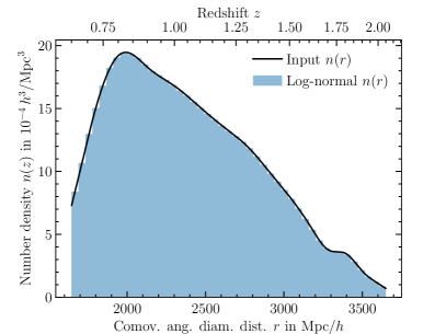
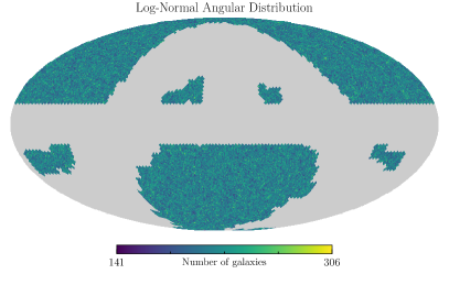
Figure 12: The plots show the approximate radial selection function and angular mask for our Euclid-like survey with one log-normal simulation.

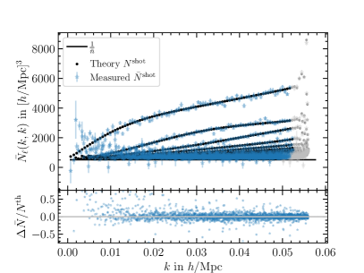
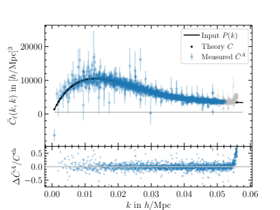
Figure 13: The plot on the left shows the shot noise and the plot on the right the SFB power spectrum similar to Fig. 9, but now for a full-sky mission like Euclid, averaged over 20 simulations, and error bars divided by $\sqrt{20}$.

As a final test for a realistic mask and selection, in this section we apply the SFB estimator to make a forecast for the spectroscopic survey of Euclid, which is an all-sky mission that covers approximately $40\text{\,}\mathrm{\char 37\relax}$ of the sky. For the number density, we adopt the reference case given in Amendola et al. (2018). We use the radial range $1645\leq\frac{r}{${\mathrm{\text{$h$}}}^{-1}\text{\,}\mathrm{Mpc}$}\leq 3650$, shown in Fig. 12. Also shown in the figure is the mask that cuts the galactic and ecliptic planes (Markovič, in prep). The number of galaxies per simulation is $\sim 68$ million.

As our primary purpose is to show the applicability of the SFB estimator, we have not updated our simulations with the parameters in Euclid Collaboration et al. (2020).

Our simulation results are shown in Fig. 13, for both shot noise-only and with a power spectrum signal with and galaxy bias $b=1.6$.

As for the other surveys, once we ignore the modes that are not fully deconvolved, we get good agreement for both cases, with $\chi^{2}_{\nu}=0.983$ for 1744 modes of one simulation.

V Conclusion

In this paper we present a new pseudo-SFB power spectrum estimator, SuperFaB. The estimator analytically accounts for shot noise, mask, and selection effects. We also investigate the impact of the local average effect and the covariance matrix.

SuperFaB works by performing the radial transform before the angular transform, similar to Leistedt et al. (2012). In the radial direction the galaxies are treated as point-particles so that no radial pixel window needs correction. The angular transform is performed using HEALPix (Górski et al., 2005; Zonca et al., 2019).

Furthermore, we derive the radial eigenmodes with potential boundary conditions at $r_{\mathrm{min}}$ and $r_{\mathrm{max}}$, as suggested by Samushia (2019). The boundary at $r_{\mathrm{min}}\neq 0$ eliminates the need for bandpower-binning in the radial direction, the boundary at $r_{\mathrm{max}}$ discretizes the measured modes $k_{n\ell}$ for integer $n$ and $\ell$.

We demonstrate that SuperFaB will be able to analyze all large-scale modes of upcoming wide and deep galaxy surveys such as Roman, SPHEREx, and Euclid.

We also review the SFB power spectrum theory and provide intuition using the Limber approximation. Notably, redshift-dependence of the power spectrum and bias factors primarily enter as the interplay between $k$ and $\ell$ modes, such that $r\sim(\ell+0.5)/k$ is an approximation for the angular diameter distance. We leave a more precise and detailed analysis for the projection of the 3D power spectrum to SFB space and the connection with cosmological parameters for a future paper.

We also leave for a future paper the extension of the estimator to cross-correlations between samples with differing selection functions.

Since the SFB power spectrum is uniquely suited for all-sky surveys, we expect a particularly intriguing application of SuperFaB will be intensity mapping at high redshift, and we look forward to this possibility.

For surveys covering a compact area on the sky we can introduce boundary conditions to the angular basis functions as well, as pointed out by Samushia (2019). This would significantly reduce the size of the computational problem in these cases.

Appendix A Useful formulae

For any function $f({\bm{k}})$

$$\int k^{2}\mathrm{d}{k}\,\mathrm{d}^{2}{\hat{\bm{k}}}\,\delta^{D}({\bm{k}}-{\bm{k}}^{\prime})\,f({\bm{k}})$$

$$=\int\mathrm{d}{k}\,\delta^{D}(k-k^{\prime})\int\mathrm{d}^{2}{\hat{\bm{k}}}\,\delta^{D}({\hat{\bm{k}}}-{\hat{\bm{k}}}^{\prime})\,f({\bm{k}})\,.$$ (106)

Therefore,

$$\delta^{D}({\bm{k}}-{\bm{k}}^{\prime}) =k^{-2}\,\delta^{D}(k-k^{\prime})\,\delta^{D}({\hat{\bm{k}}}-{\hat{\bm{k}}}^{\prime})\,.$$ (107)

Furthermore,

$$\frac{1}{r}\,\delta^{D}\!\left(\frac{1}{r}-\frac{1}{r_{0}}\right) =r\,\delta^{D}\!\left(r-r_{0}\right)\,.$$ (108)

Spherical Bessel functions and spherical harmonics satisfy orthogonality relations

$$\delta^{D}(k-k^{\prime}) =\frac{2kk^{\prime}}{\pi}\int_{0}^{\infty}\mathrm{d}{r}\,r^{2}\,j_{\ell}(kr)\,j_{\ell}(k^{\prime}r)\,,$$ (109)

$$\delta^{K}_{\ell\ell^{\prime}}\delta^{K}_{mm^{\prime}} =\int\mathrm{d}{\Omega}_{{\hat{\bm{r}}}}\,Y_{\ell m}({\hat{\bm{r}}})\,Y^{*}_{\ell^{\prime}m^{\prime}}({\hat{\bm{r}}})\,.$$ (110)

Spherical harmonics can be expressed in terms of a complex exponential and real associated Legendre functions $\mathrm{P}_{\ell}^{m}(x)$ as

$$Y_{\ell m}({\hat{\bm{r}}}) =e^{im\phi}\left(\frac{(\ell-m)!(2\ell+1)}{4\pi\left(\ell+m\right)!}\right)^{\frac{1}{2}}\mathrm{P}_{\ell}^{m}\!\left(\cos\theta\right).$$ (111)

The completeness relation is

$$\sum_{\ell m}Y_{\ell m}({\hat{\bm{r}}})\,Y^{*}_{\ell m}({\hat{\bm{r}}}^{\prime}) =\delta^{D}({\hat{\bm{r}}}-{\hat{\bm{r}}}^{\prime})\,.$$ (112)

Rayleigh’s formula decomposes the plane waves into spherical Bessels and spherical harmonics,

$$e^{i{\bm{q}}\cdot{\bm{r}}} =4\pi\sum_{\ell^{\prime},m^{\prime}}i^{\ell^{\prime}}j_{\ell^{\prime}}(qr)\,Y^{*}_{\ell^{\prime}m^{\prime}}({\hat{\bm{q}}})\,Y_{\ell^{\prime}m^{\prime}}({\hat{\bm{r}}})\,.$$ (113)

Legendre polynomials can be expressed as a sum over spherical harmonics as

$$\mathcal{P}_{\ell}({\hat{\bm{k}}}\cdot{\hat{\bm{r}}}) =\frac{4\pi}{2\ell+1}\sum_{m}Y_{\ell m}({\hat{\bm{k}}})\,Y_{\ell m}^{*}({\hat{\bm{r}}})\,.$$ (114)

Flipping the sign of the component angular momentum or the direction of the argument to spherical harmonics gives

$$Y^{*}_{\ell m}({\hat{\bm{r}}}) =(-1)^{m}Y_{\ell,-m}({\hat{\bm{r}}})\,,$$ (115)

$$Y_{\ell m}(-{\hat{\bm{r}}}) =(-1)^{\ell}Y_{\ell,m}({\hat{\bm{r}}})\,.$$ (116)

The Gaunt factor is

$$\mathcal{G}^{\ell LL_{1}}_{mMM_{1}} =\int\mathrm{d}^{2}{\hat{\bm{r}}}\,Y_{\ell m}({\hat{\bm{r}}})\,Y_{LM}({\hat{\bm{r}}})\,Y_{L_{1}M_{1}}({\hat{\bm{r}}})\,,$$ (117)

and it can be expressed in terms of Wigner-$3j$ symbols,

$$\mathcal{G}^{\ell LL_{1}}_{mMM_{1}} =\left(\frac{(2\ell+1)(2L+1)(2L_{1}+1)}{4\pi}\right)^{\frac{1}{2}}\begin{pmatrix}\ell&L&L_{1}\\ 0&0&0\end{pmatrix}$$

$$\quad\times\begin{pmatrix}\ell&L&L_{1}\\ m&M&M_{1}\end{pmatrix}\,.$$ (118)

The Wigner $3j$ symbols obey an orthogonality relation

$$\sum_{mM}\begin{pmatrix}\ell&L&L_{1}\\ m&M&M_{1}\end{pmatrix}\begin{pmatrix}\ell&L&L_{2}\\ m&M&M_{2}\end{pmatrix} =\frac{\delta^{K}_{L_{1}L_{2}}\delta^{K}_{M_{1}M_{2}}\delta^{T}(\ell,L,L_{1})}{2L_{1}+1}\,,$$ (119)

where $\delta^{T}(\ell,L,L_{1})$ enforces the triangle relation that is also obeyed by the 3$j$-symbols. That is, the Gaunt factor is only nonzero when

$$m+M+M_{1}=0\,,$$ (120)

$$|\ell-L|\leq L_{1}\leq\ell+L\,.$$ (121)

Assuming the triangle condition is satisfied, for even $J=\ell+L+L_{1}$ we have

$$\begin{pmatrix}\ell&L&L_{1}\\ 0&0&0\end{pmatrix} =(-1)^{\frac{1}{2}J}\left(\frac{(J-2\ell)!(J-2L)!(J-2L_{1})!}{(J+1)!}\right)^{\frac{1}{2}}$$

$$\quad\times\frac{\left(\frac{1}{2}J\right)!}{\left(\frac{1}{2}J-\ell\right)!\left(\frac{1}{2}J-L\right)!\left(\frac{1}{2}J-L_{1}\right)!}\,,$$ (122)

for odd $J=\ell+L+L_{1}$, those $3j$’s vanish when $m=M=M_{1}=0$.

Appendix B The Laplacian in an expanding universe

We use the SFB decomposition because that correlates radial and angular modes of the same scale. Here we show that the Laplacian in a flat expanding universe takes the form Eq. 22.

The flat Robertson-Walker metric is

$$ds^{2} =-dt^{2}+a^{2}\left[dr^{2}+r^{2}d\theta^{2}+r^{2}\sin^{2}\!\theta\,d\phi^{2}\right]\,,$$ (123)

where $r$ is the comoving coordinate, and the metric has the non-zero Christoffel symbols

$$\Gamma^{0}_{11} =a^{2}H\,, \Gamma^{0}_{22} =a^{2}r^{2}H\,, \Gamma^{0}_{33} =a^{2}r^{2}\sin^{2}\!\theta\,H\,,$$

$$\Gamma^{1}_{01} =\Gamma^{1}_{10}=H\,, \Gamma^{1}_{22} =-r\,, \Gamma^{1}_{33} =-r\sin^{2}\!\theta\,,$$

$$\Gamma^{2}_{02} =\Gamma^{2}_{20}=H\,, \Gamma^{2}_{12} =\Gamma^{2}_{21}=\frac{1}{r}\,, \Gamma^{2}_{33} =-\cos\theta\sin\theta\,,$$

$$\Gamma^{3}_{03} =\Gamma^{3}_{30}=H\,, \Gamma^{3}_{13} =\Gamma^{3}_{31}=\frac{1}{r}\,, \Gamma^{3}_{23} =\Gamma^{3}_{32}=\frac{\cos\theta}{\sin\theta}\,.$$

Therefore,

$$g^{\mu\nu}\Gamma^{0}_{\mu\nu} =3H\,,$$ (124)

$$g^{\mu\nu}\Gamma^{1}_{\mu\nu} =-2\,a^{-2}\,r^{-1}\,,$$ (125)

$$g^{\mu\nu}\Gamma^{2}_{\mu\nu} =-a^{-2}\,r^{-2}\,\frac{\cos\theta}{\sin\theta}\,,$$ (126)

$$g^{\mu\nu}\Gamma^{3}_{\mu\nu} =0\,.$$ (127)

The d’Alembertian operator for a scalar $f$ is

$$\Box f =g^{\mu\nu}\,f_{:\mu\nu}$$

$$=g^{\mu\nu}\left(\partial_{\mu}\partial_{\nu}-\Gamma^{\sigma}_{\mu\nu}\partial_{\sigma}\right)f$$

$$=\bigg{[}-\partial_{0}^{2}+a^{-2}\,\partial_{1}^{2}+a^{-2}r^{-2}\,\partial_{2}^{2}+a^{-2}r^{-2}\sin^{-2}\!\theta\,\partial_{3}^{2}$$

$$\quad-3H\,\partial_{0}+2\,a^{-2}r^{-1}\,\partial_{1}+a^{-2}r^{-2}\,\frac{\cos\theta}{\sin\theta}\,\partial_{2}\bigg{]}f$$

$$=\bigg{[}-\partial_{0}^{2}-3H\,\partial_{0}+a^{-2}\bigg{(}\partial_{1}^{2}+r^{-2}\,\partial_{2}^{2}+r^{-2}\sin^{-2}\!\theta\,\partial_{3}^{2}$$

$$\quad+2\,r^{-1}\,\partial_{1}+r^{-2}\,\frac{\cos\theta}{\sin\theta}\,\partial_{2}\bigg{)}\bigg{]}f\,.$$ (128)

Identifying the term in parentheses as given by Eq. 22, we get

$$\Box f =\left[-\partial_{0}^{2}-3H\,\partial_{0}+a^{-2}\nabla^{2}\right]f$$ (129)

in a flat expanding universe. We can also write Eq. 129 as

$$\Box f =\left[-a^{-3}\partial_{t}\!\left(a^{3}\,\partial_{t}\right)+a^{-2}\nabla^{2}\right]f\,.$$ (130)

The eigenfunctions to the d’Alembertian are, therefore, separable. If we write an eigenfunction

$$f(t,r,{\hat{\bm{r}}})=p(t)\,g(r)\,h({\hat{\bm{r}}})$$ (131)

with

$$\nabla^{2}[g(r)\,h({\hat{\bm{r}}})]=-k^{2}\,g(r)\,h({\hat{\bm{r}}})\,,$$ (132)

then

$$0 =a^{-3}\,\partial_{t}\!\left(a^{3}\,\partial_{t}p\right)+\left[a^{-2}k^{2}-\lambda^{2}\right]p\,,$$ (133)

where $-\lambda^{2}$ is the eigenvalue of the d’Alembertian. Since $ar$ is the angular diameter distance and $r$ is the comoving distance (also comoving angular diameter distance), we can call $k$ a comoving mode.

Appendix C Limber’s Approximation

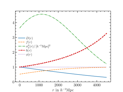
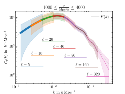
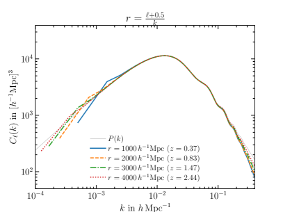
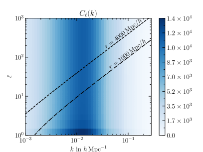
Figure 14: Top left: Linear growth factor $D(r)$, linear growth rate $f(r)$, velocity dispersion $\sigma_{u}^{2}=\sigma_{v}^{2}/(aH)^{2}$, galaxy bias $b(r)=b_{0}/D(r)$ where $b_{0}=1$, and selection function $\phi(r)$ defined in Eq. 18. Top right: The SFB power spectrum in the Limber approximation closely traces the 3D power spectrum. However, for a given perpendicular mode $\ell$ and redshift range, only a part of the power spectrum is measured. The horizontal lines show the range of $k$ modes that a given $\ell$ mode is able to measure for a survey within $1000\leq\frac{r}{h^{-1}{\rm Mpc}}\leq 4000$, and the shaded bands show an estimate for the $1\sigma$ measurement uncertainty for that particular $\ell$-mode. Bottom left: Here, each line fixes the redshift, and all $\ell$ modes are used. The Kaiser effect is not visible due to the Limber approximation becoming invalid on large scales. Bottom right: Here we show the SFB power spectrum on a grid of $\ell$-$k$ modes. Within the Limber approximation, the SFB power spectrum can be measured within a band such that $r\simeq\left(\ell+\frac{1}{2}\right)/\,k$ is within the survey. Outside this band we expect the Limber approximation to be too inaccurate even for the qualitative reasoning that is our objective here, and we leave a detailed treatment to a future paper.

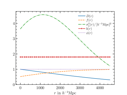
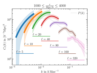
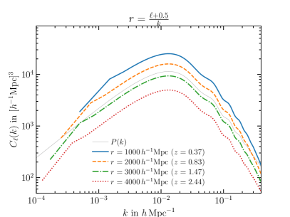
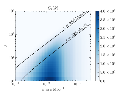
Figure 15: Same as Fig. 14, except that the linear galaxy bias is now constant $b(r)=1.8$. As a result, the redshift evolution of the linear growth factor $D(r)$ is no longer cancelled by the bias. Top right: At a fixed $\ell$, larger-scale modes are probed at higher redshift where the growth factor is smaller. Thus, compared to Fig. 14, each $\ell$-segment appears tilted. Bottom left: The redshift evolution of the linear growth factor $D(r)$ causes a shift in the power spectrum amplitude with the Limber ratio $r=(\ell+\frac{1}{2})\,/\,k$. Bottom right: High-$\ell$ modes are suppressed because they primarily probe the high redshifts.

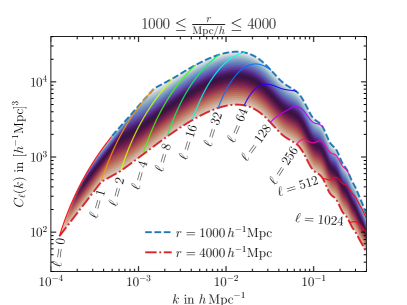
Figure 16: Here we combine the top right and bottom left plots in Fig. 15 to show the region that the SFB power spectrum probes in the Limber approximation for a given redshift range and linear power spectrum evolution.

In this section we aim to gain some intuition for the SFB power spectrum in Eq. 21 by applying a type of Limber approximation. We stress that the approximation used here is inadequate as a precise model and is only intended for the purpose of gaining intuition, especially for how redshift evolution is encoded in the SFB power spectrum at high $\ell$. To do so, we will also approximate the effect of the FoG. We write Eqs. 9 and 10 acting on a spherical Bessel function as

$$\widetilde{A}_{\mathrm{RSD}}(-iq\partial_{qr},-i\partial_{qr},r)\,j_{\ell}(qr)$$

$$=e^{\frac{1}{2}\sigma_{u}^{2}q^{2}\partial_{qr}^{2}}\left(1-\beta\partial_{qr}^{2}\right)j_{\ell}(qr)\,.$$ (134)

The second derivative is obtained exactly via a recursion relation for the derivative of Spherical Bessel function,

$$\left(1-\beta\partial_{qr}^{2}\right)j_{\ell}(qr) =\left(1-\beta f^{\ell}_{0}\right)j_{\ell}(qr)-\beta f^{\ell}_{-2}\,j_{\ell-2}(qr)$$

$$\quad-\beta f^{\ell}_{2}\,j_{\ell+2}(qr)$$ (135)

$$=\sum_{\Delta\ell}\left(\delta^{K}_{\Delta\ell,0}-\beta f^{\ell}_{\Delta\ell}\right)j_{\ell+\Delta\ell}(qr)\,,$$ (136)

where the only non-zero $f_{\Delta\ell}^{\ell}$ are

$$f_{-2}^{\ell} =\frac{\ell(\ell-1)}{(2\ell-1)(2\ell+1)}\,,$$ (137)

$$f_{0}^{\ell} =-\frac{2\ell^{2}+2\ell-1}{(2\ell-1)(2\ell+3)}\,,$$ (138)

$$f_{2}^{\ell} =\frac{(\ell+1)(\ell+2)}{(2\ell+1)(2\ell+3)}\,.$$ (139)

The FoG term acting on the spherical Bessel function is a convolution

$$\widetilde{A}_{\mathrm{FoG}}(-iq\partial_{qr})\,j_{\ell}(qr) =\int\frac{\mathrm{d}k}{2\pi}\,e^{ikqr}\,\widetilde{A}_{\mathrm{FoG}}(qk)\,\widetilde{j}_{\ell}(k)$$

$$=\int\mathrm{d}y\,A_{\mathrm{FoG}}(r-y)\,j_{\ell}(qy)$$ (140)

$$=\int\mathrm{d}y\,\frac{1}{\sqrt{2\pi}\,\sigma_{u}}\,e^{-\frac{(r-y)^{2}}{2\sigma_{u}^{2}}}\,j_{\ell}(qy)\,,$$ (141)

where the tilde signify Fourier transforms, and we took the inverse transform of Eq. 10 (see e.g. Grasshorn Gebhardt and Jeong, 2020). As a first approximation, if the frequency $q$ is low, then the convolution will have little effect. If the frequency is high, the convolution will erase the oscillations to vanish. That is, we approximate

$$\widetilde{A}_{\mathrm{FoG}}(-iq\partial_{qr})\,j_{\ell}(qr) \approx e^{-\frac{1}{2}\sigma_{u}^{2}q^{2}}\,j_{\ell}(qr)\,.$$ (142)

We are now in a position to apply a version of Limber’s approximation. The first-order result from LoVerde and Afshordi (2008) can be written as

$$J_{\nu}(kr) \simeq\delta^{D}\!\left(kr-\nu\right)\,,$$ (143)

where $J_{\nu}(x)$ is the Bessel function. Therefore, for a spherical Bessel function $j_{\ell}(x)=\sqrt{\pi/2x}\,J_{\ell+\frac{1}{2}}(x)$ we get

$$j_{\ell}(kr) \simeq\sqrt{\frac{\pi}{2rk}}\,\frac{1}{k}\,\delta^{D}\!\left(r-\frac{\ell+\frac{1}{2}}{k}\right)$$ (144)

to first order. Eq. 144 is valid only when all other functions are slowly-varying compared to the frequency of the spherical Bessel, and the integration should be over a wide interval. However, in the special case that one has two spherical Bessel functions, applying Eq. 144 reproduces Eq. 109, and that leads to the Limber approximation in the context of smooth power spectra integrated over a redshift bin (also see Jeong et al., 2009, their Appendix C). For simplicity we will refer to this as the Limber approximation. The Limber approximation Eq. 144 needs to be used with care, and we will list some of the caveats throughout this section. Then, Sections II.2 and 19 become

$$\mathcal{W}_{\ell}(k,q) =\frac{2qk}{\pi}\int\mathrm{d}r\,r^{2}\,\phi(r)\,D(r)\,b(r,q)\,j_{\ell}(kr)$$

$$\quad\times\,e^{-\frac{1}{2}\sigma_{u}^{2}q^{2}}\sum_{\Delta\ell}\left(\delta^{K}_{\Delta\ell,0}-\beta f^{\ell}_{\Delta\ell}\right)j_{\ell+\Delta\ell}(qr)$$ (145)

$$=\sqrt{\frac{q}{k}}\,\phi\!\left(\frac{\ell+\frac{1}{2}}{k}\right)D\!\left(\frac{\ell+\frac{1}{2}}{k}\right)b\!\left(\frac{\ell+\frac{1}{2}}{k},q\right)$$

$$\quad\times\,e^{-\frac{1}{2}\sigma_{u}^{2}q^{2}}\sum_{\Delta\ell}\left(\delta^{K}_{\Delta\ell,0}-\beta f^{\ell}_{\Delta\ell}\right)$$

$$\quad\times\,\delta^{D}\!\left(q-\frac{\ell+\Delta\ell+\frac{1}{2}}{\ell+\frac{1}{2}}\,k\right)\,.$$ (146)

Since the Limber approximation is only applicable for large $\ell$, we further assume $\Delta\ell\ll\ell$. Then,

$$\mathcal{W}_{\ell}(k,q) =\delta^{D}\!\left(q-k\right)\phi\!\left(\frac{\ell+\frac{1}{2}}{k}\right)D\!\left(\frac{\ell+\frac{1}{2}}{k}\right)b\!\left(\frac{\ell+\frac{1}{2}}{k},k\right)$$

$$\quad\times e^{-\frac{1}{2}\sigma_{u}^{2}k^{2}}\sum_{\Delta\ell}\left(\delta^{K}_{\Delta\ell,0}-\beta f^{\ell}_{\Delta\ell}\right).$$ (147)

Therefore, the SFB power spectrum Eq. 21 in the Limber approximation is

$$C_{\ell}(k,k^{\prime}) =P(k)\,e^{-\sigma_{u}^{2}k^{2}}\,\delta^{D}\!\left(k-k^{\prime}\right)$$

$$\quad\times\phi^{2}\!\left(\frac{\ell+\frac{1}{2}}{k}\right)D^{2}\!\left(\frac{\ell+\frac{1}{2}}{k}\right)b^{2}\!\left(\frac{\ell+\frac{1}{2}}{k},k\right)$$

$$\quad\times\left[1-\beta\left(f_{-2}^{\ell}+f_{0}^{\ell}+f_{2}^{\ell}\right)\right]^{2}.$$ (148)

The exponential is the suppression due to the FoG. The Dirac-delta function shows that even with redshift-evolution most of the power is on the diagonal $k=k^{\prime}$, as for a non-evolving universe. Redshift evolution manifests itself mainly through the interplay between $\ell$ and $k$ such that in the Limber approximation the ratio

$$r =\frac{\ell+\frac{1}{2}}{k}$$ (149)

is the comoving angular diameter distance. For example, if the scale $k$ is fixed, then changing the angular scale $\ell$ corresponds to changing the redshift. However, we caution the reader that Eq. 149 comes from the approximation Eq. 144, and a detailed treatment especially at high $k$ is needed in general. We note that primordial non-Gaussianity will lead to a scale-dependent bias that will be absorbed directly in the bias term on the second line. Finally, the last line in Appendix C accounts for the linear Kaiser effect.

In Fig. 14 we show the SFB power spectrum in the Limber approximation. We define $C_{\ell}(k)$ such that $C_{\ell}(k,k^{\prime})=\delta^{D}(k-k^{\prime})\,C_{\ell}(k)$. For the galaxy bias we choose $b(r,k)=b_{0}/D(r)$ with $b_{0}=1$ so that the bias and linear growth factor cancel, and our selection function is a constant $\phi(r)=1$ for illustration. The top left panel shows the inputs to our calculation.

The top right panel of Fig. 14 shows the SFB power spectrum for several fixed $\ell$ modes. The shaded areas correspond to the $1\sigma$ measurement uncertainty estimated via

$$\Delta C_{\ell}(k) =\sqrt{\frac{2}{2\ell+1}}\left(C_{\ell}(k)+\frac{1}{{\bar{n}}}\right),$$ (150)

(Pratten and Munshi, 2013). Since $\ell$ corresponds to perpendicular wave modes, at small $r$ the corresponding $k$ modes are large, and at large $r$ the corresponding $k$ modes are small. Therefore, at a constant $\ell$, the SFB power spectrum as a function of $k$ sweeps through both redshift and $k$ modes, measuring a redshift corresponding to $r\simeq$4000\text{\,}{\mathrm{\text{$h$}}}^{-1}\text{\,}\mathrm{Mpc}$$ at lower $k$, and a redshift corresponding to $r\simeq$1000\text{\,}{\mathrm{\text{$h$}}}^{-1}\text{\,}\mathrm{Mpc}$$ at higher $k$.

Consequently, in the $\ell$-$k$ plane, only a band of modes can be measured, as illustrated in the bottom right plot of Fig. 14. Fixing the redshift, which is possible in the Limber approximation, results in a bona-fide power spectrum measurement, as illustrated in the bottom left panel.

In the Limber approximation, the SFB power spectrum does not exhibit a strong Kaiser effect. We attribute this to our approximations being inadequate for such analysis, and we refer the reader to Yoo and Desjacques (2013); Munshi et al. (2016) for further details.

Because Eq. 149 relates the $\ell$ and $k$ modes to a definite redshift, we can only measure a band of modes. We illustrate this in the bottom right panel of Fig. 14. More generally, Eq. 149 is valid only approximately, and the detailed treatment outside this band is dependent on the exact choice of basis functions.

The choice $b(r,q)\,\propto\,D^{-1}(r)$ results in linear bias and linear growth cancelling each other. In general, this may not be the case, and we illustrate redshift evolution by setting the bias constant, $b(r,q)=1.8$, in Fig. 15. Because for fixed $\ell$ larger-scale modes $k$ correspond to higher redshift, the linear growth evolution tilts each $\ell$-segment of the power spectrum in the top right panel. The bottom left panel shows the power spectrum at fixed redshift according to the Limber ratio Eq. 149, sweeping through $\ell$.

Each segment in the top right panel of Fig. 15 crosses the lines in the bottom left panel. We illustrate this further in Fig. 16.

We hope that this appendix gives some insight into how the SFB power spectrum works. However, we stress again that the approximations made here are inadequate for a full cosmological analysis, and the reader should keep this caveat in mind.

Appendix D Radial spherical Fourier-Bessel modes with potential boundary conditions

In this appendix we derive the radial basis functions of the Laplacian with potential boundary conditions at $r_{\mathrm{min}}$ and $r_{\mathrm{max}}$.

We first isolate the radial part of Eq. 22. Writing

$$f({\bm{r}}) =g(r)\,h({\hat{\bm{r}}})\,,$$ (151)

we require

$$-k^{2}gh =\frac{h}{r^{2}}\,\frac{\partial}{\partial r}\left(r^{2}\,\frac{\partial g}{\partial r}\right)+g\,\nabla^{2}h\,.$$ (152)

Given the spherical harmonic solution for the angular term $h$,

$$\nabla^{2}h =-\frac{\ell(\ell+1)}{r^{2}}\,h\,,$$ (153)

we get

$$0 =\frac{\mathrm{d}}{\mathrm{d}r}\left(r^{2}\,\frac{\mathrm{d}g_{\ell}(kr)}{\mathrm{d}r}\right)+\big{[}(kr)^{2}-\ell(\ell+1)\big{]}\,g_{\ell}(kr)\,,$$ (154)

where we now added that the function $g$ depends on $\ell$. Our first aim is to derive the discrete spectrum of $k$ modes for a given $\ell$. We then use that to derive the form of the $g_{\ell}$. Following Fisher et al. (1995), we demand that the orthogonality relation Eq. 26 is satisfied. However, we modify the approach in Fisher et al. (1995) to integrate from $r_{\mathrm{min}}$ to $r_{\mathrm{max}}$. Eq. 154 multiplied by $g_{\ell}(kr)$ then yields

$$\int_{r_{\mathrm{min}}}^{r_{\mathrm{max}}}\mathrm{d}r\,\frac{\mathrm{d}}{\mathrm{d}r}\left(r^{2}\,\frac{\mathrm{d}g_{\ell}(kr)}{\mathrm{d}r}\right)g_{\ell}(k^{\prime}r)$$

$$=\int_{r_{\mathrm{min}}}^{r_{\mathrm{max}}}\mathrm{d}r\,\big{[}\ell(\ell+1)-(kr)^{2}\big{]}\,g_{\ell}(kr)\,g_{\ell}(k^{\prime}r)\,.$$ (155)

Subtract from this equation the same equation with $k$ and $k^{\prime}$ interchanged,

$$\big{[}k^{\prime 2}-k^{2}\big{]}\int_{r_{\mathrm{min}}}^{r_{\mathrm{max}}}\mathrm{d}r\,r^{2}\,g_{\ell}(kr)\,g_{\ell}(k^{\prime}r)$$

$$=\int_{r_{\mathrm{min}}}^{r_{\mathrm{max}}}\mathrm{d}r\,\bigg{\{}\frac{\mathrm{d}}{\mathrm{d}r}\left(r^{2}\,\frac{\mathrm{d}g_{\ell}(kr)}{\mathrm{d}r}\right)g_{\ell}(k^{\prime}r)$$

$$\quad-\frac{\mathrm{d}}{\mathrm{d}r}\left(r^{2}\,\frac{\mathrm{d}g_{\ell}(k^{\prime}r)}{\mathrm{d}r}\right)g_{\ell}(kr)\bigg{\}}\,.$$ (156)

Partial integration with the terms on the right hand side (r.h.s.) yields

$$\int\mathrm{d}r\,\frac{\mathrm{d}}{\mathrm{d}r}\!\left(kr^{2}g^{\prime}_{\ell}(kr)\right)g_{\ell}(k^{\prime}r)$$

$$=\left.kr^{2}g^{\prime}_{\ell}(kr)g_{\ell}(k^{\prime}r)\right|_{r_{\mathrm{min}}}^{r_{\mathrm{max}}}-kk^{\prime}\int\mathrm{d}r\,r^{2}\,g^{\prime}_{\ell}(kr)g^{\prime}_{\ell}(k^{\prime}r)\,.$$ (157)

Then, Eq. 156 becomes

$$\big{[}k^{\prime 2}-k^{2}\big{]}\int_{r_{\mathrm{min}}}^{r_{\mathrm{max}}}\mathrm{d}r\,r^{2}\,g_{\ell}(kr)\,g_{\ell}(k^{\prime}r)$$

$$=\left.kr^{2}g^{\prime}_{\ell}(kr)g_{\ell}(k^{\prime}r)\right|_{r_{\mathrm{min}}}^{r_{\mathrm{max}}}-\left.k^{\prime}r^{2}g^{\prime}_{\ell}(k^{\prime}r)g_{\ell}(kr)\right|_{r_{\mathrm{min}}}^{r_{\mathrm{max}}}\,.$$ (158)

The r.h.s.  will vanish for any $k$ whenever

$$0 =Akr_{\mathrm{max}}^{2}g^{\prime}_{\ell}(kr_{\mathrm{max}})-Br_{\mathrm{max}}^{2}g_{\ell}(kr_{\mathrm{max}})$$

$$\quad-akr_{\mathrm{min}}^{2}g^{\prime}_{\ell}(kr_{\mathrm{min}})+br_{\mathrm{min}}^{2}g_{\ell}(kr_{\mathrm{min}})\,.$$ (159)

for any constants $a$, $b$, $A$, and $B$.

To choose $a$, $b$, $A$, and $B$, we note that the representable field $\delta({\bm{r}})$ is written as a sum of the solutions to Eq. 154 inside the SFB volume, and we have some freedom to choose the desired behavior outside of it. Since the field inside the SFB volume satisfies the Poisson equation, it is natural to have it satisfy Laplace’s equation outside it, and demand that the solution is continuous and smooth at the boundaries. That is,

$$\delta({\bm{r}}) =\begin{cases}\sum_{\ell m}\left[a_{\ell m}\left(\frac{r}{r_{\mathrm{min}}}\right)^{\ell}+b_{\ell m}\left(\frac{r_{\mathrm{min}}}{r}\right)^{\ell+1}\right]Y_{\ell m}({\hat{\bm{r}}})\,,&\text{for }r<r_{\mathrm{min}}\,,\\ \sum_{n\ell m}\Big{[}c_{n\ell}\,j_{\ell}(k_{n\ell}\,r)+d_{n\ell}\,y_{\ell}(k_{n\ell}\,r)\Big{]}Y_{\ell m}({\hat{\bm{r}}})\,\delta_{n\ell m}\,,&\text{for }r_{\mathrm{min}}\leq r\leq r_{\mathrm{max}}\,,\\ \sum_{\ell m}\left[A_{\ell m}\left(\frac{r}{r_{\mathrm{max}}}\right)^{\ell}+B_{\ell m}\left(\frac{r_{\mathrm{max}}}{r}\right)^{\ell+1}\right]Y_{\ell m}({\hat{\bm{r}}})\,,&\text{for }r>r_{\mathrm{max}}\,,\end{cases}$$ (160)

where we defined the constants $a_{\ell m}$, $b_{\ell m}$, $c_{n\ell}$, $d_{n\ell}$, $A_{\ell m}$, and $B_{\ell m}$, and we explicitly wrote

$$g_{\ell}(kr)=c_{n\ell}\,j_{\ell}(kr)+d_{n\ell}\,y_{\ell}(kr)\,,$$ (161)

and we anticipate that the function $g_{\ell}$ will also depend on $n$. Continuity at the boundaries requires

$$a_{\ell m}+b_{\ell m} =\sum_{n}g_{\ell}(k_{n\ell}\,r_{\mathrm{min}})\,\delta_{n\ell m}\,,$$ (162)

$$A_{\ell m}+B_{\ell m} =\sum_{n}g_{\ell}(k_{n\ell}\,r_{\mathrm{max}})\,\delta_{n\ell m}\,.$$ (163)

Smoothness further requires

$$\ell\,\frac{a_{\ell m}}{r_{\mathrm{min}}}-(\ell+1)\,\frac{b_{\ell m}}{r_{\mathrm{min}}} =\sum_{n}k_{n\ell}\,g^{\prime}_{\ell}(k_{n\ell}\,r_{\mathrm{min}})\,\delta_{n\ell m}\,,$$ (164)

$$\ell\,\frac{A_{\ell m}}{r_{\mathrm{max}}}-(\ell+1)\,\frac{B_{\ell m}}{r_{\mathrm{max}}} =\sum_{n}k_{n\ell}\,g^{\prime}_{\ell}(k_{n\ell}\,r_{\mathrm{max}})\,\delta_{n\ell m}\,,$$ (165)

Now requiring $\delta({\bm{r}})$ to be finite at $r=0$ and $r=\infty$ sets $b_{\ell m}=A_{\ell m}=0$, and requiring continuity and smoothness for any $\delta_{n\ell m}$, we get

$$\ell\,g_{\ell}(k_{n\ell}\,r_{\mathrm{min}}) =k_{n\ell}\,r_{\mathrm{min}}\,g^{\prime}_{\ell}(k_{n\ell}\,r_{\mathrm{min}})\,,$$ (166)

$$-(\ell+1)\,g_{\ell}(k_{n\ell}\,r_{\mathrm{max}}) =k_{n\ell}\,r_{\mathrm{max}}\,g^{\prime}_{\ell}(k_{n\ell}\,r_{\mathrm{max}})\,.$$ (167)

These choices lead to $a=1$, $b=\ell/r_{\mathrm{min}}$, $A=1$, and $B=-(\ell+1)/r_{\mathrm{max}}$ in Eq. 159, which shows that the conditions Eqs. 166 and 167 on $k_{n\ell}$ lead to an orthogonality relation for the $g_{\ell}$.

Both $j_{\ell}$ and $y_{\ell}$ satisfy the two recurrence relations

$$j^{\prime}_{\ell}(kr) =-j_{\ell+1}(kr)+\frac{\ell}{kr}\,j_{\ell}(kr)\,,$$ (168)

$$j^{\prime}_{\ell}(kr) =j_{\ell-1}(kr)-\frac{\ell+1}{kr}\,j_{\ell}(kr)\,.$$ (169)

Then, Eqs. 166 and 167 simplify to

$$c_{n\ell}\,j_{\ell+1}(k_{n\ell}\,r_{\mathrm{min}})+d_{n\ell}\,y_{\ell+1}(k_{n\ell}\,r_{\mathrm{min}}) =0\,,$$ (170)

$$c_{n\ell}\,j_{\ell-1}(k_{n\ell}\,r_{\mathrm{max}})+d_{n\ell}\,y_{\ell-1}(k_{n\ell}\,r_{\mathrm{max}}) =0\,.$$ (171)

The normalization of $g_{\ell}$ is obtained by dividing Eq. 158 by $k^{\prime 2}-k^{2}$, and taking the limit $k^{\prime}\to k=k_{n\ell}$,

$$1 =\int_{r_{\mathrm{min}}}^{r_{\mathrm{max}}}\mathrm{d}r\,r^{2}\,g^{2}_{\ell}(kr)$$

$$=\lim_{k^{\prime}\to k}\frac{\left.kr^{2}g^{\prime}_{\ell}(kr)g_{\ell}(k^{\prime}r)\right|_{r_{\mathrm{min}}}^{r_{\mathrm{max}}}-\left.k^{\prime}r^{2}g^{\prime}_{\ell}(k^{\prime}r)g_{\ell}(kr)\right|_{r_{\mathrm{min}}}^{r_{\mathrm{max}}}}{k^{\prime 2}-k^{2}}\,.$$ (172)

When $kr=k_{n\ell}r_{\mathrm{min}}$ as in Eq. 166,

$$kr\,g^{\prime}_{\ell}(kr)g_{\ell}(k^{\prime}r)-k^{\prime}r\,g^{\prime}_{\ell}(k^{\prime}r)g_{\ell}(kr)$$

$$=k^{\prime}r\,g_{\ell}(kr)\big{[}c_{n\ell}\,j_{\ell+1}(k^{\prime}r)+d_{n\ell}\,y_{\ell+1}(k^{\prime}r)\big{]}\,,$$ (173)

and when $kr=k_{n\ell}r_{\mathrm{max}}$ as in Eq. 167,

$$kr\,g^{\prime}_{\ell}(kr)g_{\ell}(k^{\prime}r)-k^{\prime}r\,g^{\prime}_{\ell}(k^{\prime}r)g_{\ell}(kr)$$

$$=-k^{\prime}r\,g_{\ell}(kr)\big{[}c_{n\ell}\,j_{\ell-1}(k^{\prime}r)+d_{n\ell}\,y_{\ell-1}(k^{\prime}r)\big{]}\,.$$ (174)

The terms in brackets vanish in the limit $k^{\prime}\to k=k_{n\ell}$ as per Eqs. 170 and 171. That is, we need limits

$$\lim_{q^{\prime}\to q}\frac{c_{n\ell}\,j_{\ell+1}(q^{\prime})+d_{n\ell}\,y_{\ell+1}(q^{\prime})}{q^{\prime 2}-q^{2}} =\frac{g_{\ell}(q)}{2q}\,,$$ (175)

$$\lim_{q^{\prime}\to q}\frac{c_{n\ell}\,j_{\ell-1}(q^{\prime})+d_{n\ell}\,y_{\ell-1}(q^{\prime})}{q^{\prime 2}-q^{2}} =-\frac{g_{\ell}(q)}{2q}\,,$$ (176)

for $q=kr_{\mathrm{min}}$ and $q=kr_{\mathrm{max}}$, respectively. Then, Eq. 172 becomes

$$1 =\frac{r^{3}_{\mathrm{max}}}{2}\,\,g^{2}_{\ell}(k_{n\ell}\,r_{\mathrm{max}})-\frac{r^{3}_{\mathrm{min}}}{2}\,g^{2}_{\ell}(k_{n\ell}\,r_{\mathrm{min}})\,.$$ (177)

Choosing $k_{n\ell}$, $c_{n\ell}$, and $d_{n\ell}$ that satisfy Eqs. 170, 171 and 177 guarantees the orthonormality of the $g_{\ell}$,

$$\int_{r_{\mathrm{min}}}^{r_{\mathrm{max}}}\mathrm{d}r\,r^{2}\,g_{\ell}(k_{n\ell}\,r)\,g_{\ell}(k_{n^{\prime}\ell}\,r) =\delta^{K}_{nn^{\prime}}\,.$$ (178)

Note that the condition $\ell=\ell^{\prime}$ is not enforced by the $g_{\ell}$. Instead, $\ell=\ell^{\prime}$ comes from the spherical harmonics, i.e., Eq. 110.

D.1 Phase factor

We are free to introduce a phase factor for the $g_{n\ell}(r)$, and we choose it so that the sign of $g_{n\ell}(r_{\mathrm{min}})$ alternates with $n$, but stays constant with $\ell$,

$$g_{n\ell}(r) =(-1)^{\left[1-\mathrm{floor}\left(\frac{1}{\ell+1}\right)\right]\left[1-\mathrm{floor}\left(\frac{1}{n}\right)\right]}\,\tilde{g}_{n\ell}(r)\,,$$ (179)

where the tilde indicates that we have not included the phase factor. This flips the sign unless either $\ell\neq 0$ or $n\neq 1$. Thus, the basis functions in Fig. 1 are obtained.

D.2 Numerical concerns

To calculate $k_{n\ell}$, solve each of Eqs. 170 and 171 for the ratio $d_{n\ell}/c_{n\ell}$, and set them equal to get

$$0 =j_{\ell-1}(k_{n\ell}\,r_{\mathrm{max}})\,y_{\ell+1}(k_{n\ell}\,r_{\mathrm{min}})$$

$$\quad-y_{\ell-1}(k_{n\ell}\,r_{\mathrm{max}})\,j_{\ell+1}(k_{n\ell}\,r_{\mathrm{min}})\,.$$ (180)

Examples for the resulting zeros and the first few basis functions are shown in Fig. 1. The ratio $d_{n\ell}/c_{n\ell}$ then follows from Eq. 170 or Eq. 171. Finally, the overall normalization is fixed by Eq. 177 up to a sign.

When $r_{\mathrm{max}}$ is large and $r_{\mathrm{min}}$ is small, the $k_{n\ell}$ may need to be computed using arbitrary precision floats, and the $g_{n\ell}$ may need to be calculated with arbitrary precision as well. Caching the result in double precision should then provide for sufficient speed for the actual transform.

Appendix E Covariance matrix simplification

In this appendix we simplify the covariance matrix Section III.9. For simplicity we ignore the local average effect. We explicitly treat the shot noise Eq. 63 because it is inhomogeneous and anisotropic. We get

$$\left\langle\delta^{W,A}_{NLM}\,\delta^{W,A,*}_{N^{\prime}L^{\prime}M^{\prime}}\right\rangle =\sum_{n_{1}\ell_{1}m_{1}}W_{NLM}^{n_{1}\ell_{1}m_{1}}\sum_{n_{2}\ell_{2}m_{2}}W_{N^{\prime}L^{\prime}M^{\prime}}^{n_{2}\ell_{2}m_{2},*}\bigg{[}\delta^{K}_{\ell_{1}\ell_{2}}\delta^{K}_{m_{1}m_{2}}\,C_{\ell_{1}n_{1}n_{2}}+\frac{1}{{\bar{n}}}\left(W^{-1}\right)_{n_{1}\ell_{1}m_{1}}^{n_{2}\ell_{2}m_{2}}\bigg{]}$$ (181)

$$=\sum_{\ell_{1}n_{1}n_{2}}C_{\ell_{1}n_{1}n_{2}}\sum_{m_{1}}W_{NLM}^{n_{1}\ell_{1}m_{1}}W^{N^{\prime}L^{\prime}M^{\prime}}_{n_{2}\ell_{1}m_{1}}+\frac{1}{{\bar{n}}}W^{N^{\prime}L^{\prime}M^{\prime}}_{NLM}\,,$$ (182)

where we used Eq. 37. Similarly, when neither density contrast has the complex conjugate attached,

$$\left\langle\delta^{W,A}_{NLM}\,\delta^{W,A}_{N^{\prime}L^{\prime}M^{\prime}}\right\rangle =(-1)^{M^{\prime}}\sum_{\ell_{1}n_{1}n_{2}}C_{\ell_{1}n_{1}n_{2}}\sum_{m_{1}}W_{NLM}^{n_{1}\ell_{1}m_{1}}W^{N^{\prime}L^{\prime},-M^{\prime}}_{n_{2}\ell_{1}m_{1}}+\frac{(-1)^{M^{\prime}}}{{\bar{n}}}W^{N^{\prime}L^{\prime},-M^{\prime}}_{NLM}\,,$$ (183)

where we used Eq. 115. Therefore, both terms in Section III.9 are of the form

$$\frac{1}{(2\ell+1)(2L+1)}\sum_{mM}\left\langle\delta^{W,A}_{n\ell m}\delta^{W,A,*}_{NLM}\right\rangle\left\langle\delta^{{W,A}}_{n^{\prime}\ell m}\delta^{{W,A},*}_{N^{\prime}LM}\right\rangle$$

$$=\frac{1}{(2\ell+1)(2L+1)}\sum_{mM}\left[\sum_{\ell_{1}n_{1}n_{2}}C_{\ell_{1}n_{1}n_{2}}\sum_{m_{1}}W_{n\ell m}^{n_{1}\ell_{1}m_{1}}W^{NLM}_{n_{2}\ell_{1}m_{1}}+\frac{1}{{\bar{n}}}W^{NLM}_{n\ell m}\right]$$

$$\quad\times\left[\sum_{\ell_{3}n_{3}n_{4}}C_{\ell_{3}n_{3}n_{4}}\sum_{m_{3}}W_{n^{\prime}\ell m}^{n_{3}\ell_{3}m_{3},*}W^{N^{\prime}LM,*}_{n_{4}\ell_{3}m_{3}}+\frac{1}{{\bar{n}}}W^{N^{\prime}LM,*}_{n^{\prime}\ell m}\right]$$ (184)

$$=\frac{1}{(2\ell+1)(2L+1)}\sum_{mM}\Bigg{[}\sum_{\ell_{1}n_{1}n_{2}}C_{\ell_{1}n_{1}n_{2}}\sum_{m_{1}}W_{n\ell m}^{n_{1}\ell_{1}m_{1}}W^{NLM}_{n_{2}\ell_{1}m_{1}}\sum_{\ell_{3}n_{3}n_{4}}C_{\ell_{3}n_{3}n_{4}}\sum_{m_{3}}W_{n^{\prime}\ell m}^{n_{3}\ell_{3}m_{3},*}W^{N^{\prime}LM,*}_{n_{4}\ell_{3}m_{3}}$$

$$\quad+\frac{1}{{\bar{n}}}W^{NLM}_{n\ell m}\frac{1}{{\bar{n}}}W^{N^{\prime}LM,*}_{n^{\prime}\ell m}+\frac{1}{{\bar{n}}}W^{N^{\prime}LM,*}_{n^{\prime}\ell m}\sum_{\ell_{1}n_{1}n_{2}}C_{\ell_{1}n_{1}n_{2}}\sum_{m_{1}}W_{n\ell m}^{n_{1}\ell_{1}m_{1}}W^{NLM}_{n_{2}\ell_{1}m_{1}}+\left\langle n\leftrightarrow n^{\prime},N\leftrightarrow N^{\prime}\right\rangle^{*}\Bigg{]}$$ (185)

$$=A_{1}{}^{LNN^{\prime}}_{\ell nn^{\prime}}+A_{2}{}^{LNN^{\prime}}_{\ell nn^{\prime}}+A_{2}{}^{LN^{\prime}N}_{\ell n^{\prime}n}+A_{3}{}^{LNN^{\prime}}_{\ell nn^{\prime}}\,.$$ (186)

Using Eq. 37, we get

$$A_{1}{}^{LNN^{\prime}}_{\ell nn^{\prime}} =\frac{1}{(2\ell+1)(2L+1)}\sum_{\ell_{1}n_{1}n_{2}}C_{\ell_{1}n_{1}n_{2}}\sum_{\ell_{3}n_{3}n_{4}}C_{\ell_{3}n_{3}n_{4}}\,W_{4}\!\!\begin{pmatrix}\ell_{1}&L&\ell_{3}&\ell\\ n_{1}&N&n_{4}&n^{\prime}\\ n_{2}&N^{\prime}&n_{3}&n\end{pmatrix},$$ (187)

and

$$A_{2}{}^{LNN^{\prime}}_{\ell nn^{\prime}} =\frac{1}{{\bar{n}}}\,\frac{1}{(2\ell+1)(2L+1)}\sum_{\ell_{1}n_{1}n_{2}}C_{\ell_{1}n_{1}n_{2}}\,W_{3}\!\!\begin{pmatrix}\ell_{1}&L&\ell\\ n_{1}&N&n^{\prime}\\ n_{2}&N^{\prime}&n\end{pmatrix},$$ (188)

and

$$A_{3}{}^{LNN^{\prime}}_{\ell nn^{\prime}} =\frac{1}{{\bar{n}}^{2}}\,\frac{1}{(2\ell+1)(2L+1)}\,W_{2}\!\!\begin{pmatrix}L&\ell\\ N&n^{\prime}\\ N^{\prime}&n\end{pmatrix}=\frac{1}{{\bar{n}}^{2}}\,\frac{1}{2\ell+1}\,\mathcal{M}^{LNN^{\prime}}_{\ell nn^{\prime}}\,.$$ (189)

The $W_{k}$ symbols are defined in Eq. 191 and discussed in Appendix F. Then Section III.9 becomes

$$V^{W}{}_{\ell nn^{\prime}}^{LNN^{\prime}} =A_{1}{}^{LNN^{\prime}}_{\ell nn^{\prime}}+A_{2}{}^{LNN^{\prime}}_{\ell nn^{\prime}}+A_{2}{}^{LN^{\prime}N}_{\ell n^{\prime}n}+A_{3}{}^{LNN^{\prime}}_{\ell nn^{\prime}}+\left\langle N\leftrightarrow N^{\prime}\right\rangle.$$ (190)

The $A_{1}$ term dominates if the power spectrum is much larger than the shot noise, and $A_{3}$ dominates if shot noise is larger.

Appendix F Chains of window functions

Throughout the paper, we find that traces of density-contrast window coupling matrices $W$ appear with summations over the azimuthal modes $m$. That is, we find tensors $W_{k}$ of the form

$$W_{k}\!\!\begin{pmatrix}\ell_{1}&\ell_{2}&\ldots&\ell_{k}\\ n_{1}&n_{2}&\ldots&n_{k}\\ n^{\prime}_{1}&n^{\prime}_{2}&\ldots&n^{\prime}_{k}\end{pmatrix} =\sum_{m_{1}m_{2}\ldots m_{k}}W_{n^{\prime}_{k}\ell_{k}m_{k}}^{n_{1}\ell_{1}m_{1}}\,W_{n^{\prime}_{1}\ell_{1}m_{1}}^{n_{2}\ell_{2}m_{2}}\cdots W_{n^{\prime}_{k-1}\ell_{k-1}m_{k-1}}^{n_{k}\ell_{k}m_{k}}\,.$$ (191)

This starts with a single window function Eq. 64 ($k=1$) for shot noise, two window functions Eqs. 51 and 189 ($k=2$) for the pseudo power spectrum mixing matrix and shot noise covariance, three window functions Sections III.8 and 188 for part of the local average effect and covariance calculations, four window functions Eq. 187. If we were to include the local average effect in the covariance, then $k=5$ and $k=6$ would also occur.

The $W_{k}$ are real, which is trivially shown by substituting each window with its definition Section III.2 and using Eq. 114. Also, cyclical permutations of the argument columns leave $W_{k}$ invariant, and anticyclical permutations leave it invariant if all $n_{i}$ and $n^{\prime}_{i}$ are switched as well. That is,

$$W_{k}\!\!\begin{pmatrix}\ell_{1}&\ell_{2}&\ldots&\ell_{k}\\ n_{1}&n_{2}&\ldots&n_{k}\\ n^{\prime}_{1}&n^{\prime}_{2}&\ldots&n^{\prime}_{k}\end{pmatrix}=W_{k}\!\!\begin{pmatrix}\ell_{k}&\ell_{1}&\ldots&\ell_{k-1}\\ n_{k}&n_{1}&\ldots&n_{k-1}\\ n^{\prime}_{k}&n^{\prime}_{1}&\ldots&n^{\prime}_{k-1}\end{pmatrix}=W_{k}\!\!\begin{pmatrix}\ell_{k}&\ell_{k-1}&\ldots&\ell_{1}\\ n^{\prime}_{k}&n^{\prime}_{k-1}&\ldots&n^{\prime}_{1}\\ n_{k}&n_{k-1}&\ldots&n_{1}\end{pmatrix}.$$ (192)

The first equality trivially follows from the definition Eq. 191, and the second from applying Eq. 37 to all the windows.

F.1 Evaluation for separable window function

For a separable window $W({\bm{r}})=\phi(r)\,W({\hat{\bm{r}}})$, Eq. 40 becomes

$$W_{n^{\prime}\ell^{\prime}m^{\prime}}^{n\ell m} =I_{n^{\prime}\ell^{\prime}}^{n\ell}\,W_{\ell^{\prime}m^{\prime}}^{\ell m}\,,$$ (193)

where

$$I_{n^{\prime}\ell^{\prime}}^{n\ell} =\int_{r_{\mathrm{min}}}^{r_{\mathrm{max}}}\mathrm{d}r\,r^{2}\,g_{n^{\prime}\ell^{\prime}}(r)\,g_{n\ell}(r)\,\phi(r)\,,$$ (194)

$$W_{\ell^{\prime}m^{\prime}}^{\ell m} =(-1)^{m^{\prime}}\sum_{LM}\mathcal{G}^{\ell^{\prime}\ell L}_{-m^{\prime},m,M}\,W_{LM}\,,$$ (195)

where $W_{LM}$ was defined in Eq. 55. Thus, Eq. 191 is

$$W_{k}\!\!\begin{pmatrix}\ell_{1}&\ell_{2}&\ldots&\ell_{k}\\ n_{1}&n_{2}&\ldots&n_{k}\\ n^{\prime}_{1}&n^{\prime}_{2}&\ldots&n^{\prime}_{k}\end{pmatrix} =I_{n^{\prime}_{k}\ell_{k}}^{n_{1}\ell_{1}}\,I_{n^{\prime}_{1}\ell_{1}}^{n_{2}\ell_{2}}\cdots I_{n^{\prime}_{k-1}\ell_{k-1}}^{n_{k}\ell_{k}}\sum_{m_{1}m_{2}\ldots m_{k}}\,W_{\ell_{k}m_{k}}^{\ell_{1}m_{1}}\,W_{\ell_{1}m_{1}}^{\ell_{2}m_{2}}\cdots W_{\ell_{k-1}m_{k-1}}^{\ell_{k}m_{k}}\,.$$ (196)

Eq. 196 contains $\mathcal{O}\!\left(\ell^{k}\right)$ terms.