The Disparate Impact of Uncertainty:
Affirmative Action vs. Affirmative Information

Abstract

Critical decisions like hiring, college admissions, and loan approvals are guided by predictions made in the presence of uncertainty. While uncertainty imparts errors across all demographic groups, this paper shows that the types of errors vary systematically: Groups with higher average outcomes are typically assigned higher false positive rates, while those with lower average outcomes are assigned higher false negative rates. We characterize the conditions that give rise to this disparate impact and explain why the intuitive remedy to omit demographic variables from datasets does not correct it. Instead of data omission, this paper examines how data enrichment can broaden access to opportunity. The strategy, which we call “Affirmative Information,” could stand as an alternative to Affirmative Action.

JEL Codes: J7, D8, C54, C55, D6

1 Introduction

Decision-makers can inadvertently contribute to inequality as they wrestle with uncertainty. Empirical studies of child abuse cases, the criminal justice system, and hospital screenings have shown that the burden of prediction errors can fall disproportionately on the most disadvantaged subpopulations [Angwin et al., 2016; Arnold, Dobbie and Hull, 2022; Eubanks, 2018; Obermeyer et al., 2019]. This translates to systematically lower access to opportunities that are needed and deserved.

To explain biased outcomes, intuition often guides us to search for bias in the data that drive the predictions. This paper, however, shows that bias enters predictions not only through included data, but also through the absence of data. We explain how uncertainty complicates efforts to identify equally qualified candidates from different demographic groups and thereby generates disparate impacts.

In particular, we consider screening decisions in which applicants are either granted or denied an opportunity, such as a loan, based on predictions of their eventual outcomes, such as loan repayment. We show that while uncertainty affects the accuracy of predictions for all subpopulations in the data, the types of errors vary systematically. Applicants from lower-average groups tend to be assigned higher false negative rates and those from higher-average groups tend to be assigned higher false positive rates. As a result, applicants from lower-average groups are less likely to be accepted conditional on their true ability.

We show that the disparate impact of uncertainty can emerge from facially neutral prediction methods, such as screening algorithms stripped of sensitive data. Blinding decision-makers and their algorithms to sensitive demographic variables like group identifiers and their proxies is therefore not a cure. This distinguishes the disparate impact of uncertainty from traditional statistical discrimination, in which differences in access to opportunity can be traced back to the decision-makers’ choice to weigh demographic characteristics [Aigner and Cain, 1977].

Rather than relying on demographic characteristics, the disparate impact of uncertainty emerges due the mechanistic force of regression toward the mean. In the presence of uncertainty, regression toward the mean causes the overall distribution of predicted ability to contract toward the mean ability, but we show that predictions for different groups contract toward different means when the underlying data is correlated with group membership. Uncertainty pulls predictions of applicants from lower-mean groups toward lower values, causing the distribution of predictions given true ability to vary systematically by group.

Since the variables included in prediction models often explain how demographic groups are disadvantaged, the disparate impact we characterize here regularly arises in practice. In the lending context, for example, we rarely suppose that demographic characteristics actually drive observed differences in group repayment rates. Instead, demographic characteristics are correlated with financial characteristics that do drive repayment ability. When lenders include those financial characteristics in their models, they inadvertently create opportunities for uncertainty to generate disparate impacts across demographic groups.

Fortunately, it is possible for decision-makers to eliminate the disparate impact of uncertainty. To do so, we prove that at least one of the following must be true: (1) members of the lower-mean groups must be over-represented among positive classifications, OR (2) their predictions must be more accurate than those of higher-mean groups. The second prong of this mathematical result motivates us to propose a practical method to broaden access to opportunity across qualified applicants: acquire additional data about individuals in disadvantaged groups. We call this strategy “Affirmative Information.” It could promote both fairness and accuracy in the wake of the United States Supreme Court’s historic decision to strike down Affirmative Action in SFFA v. Harvard and SFFA v. UNC.

In contrast to our proposal of data enrichment, many prediction models in use today seek to achieve fairness through data omission. This paper therefore supports the growing evidence in both economics and computer science showing that blinding algorithms to demographic characteristics is an ineffective approach to fair prediction. Within this literature, Kleinberg and Mullainathan [2019]; Dwork et al. [2018]; Rambachan et al. [2020] advance theory showing that fairness considerations are best imposed after estimating the most accurate predictions, rather than before, and Kleinberg et al. [2018]; Lazar Reich and Vijaykumar [2021] demonstrate this principle empirically in real-world settings. Our paper aligns with recent evidence that data collection can serve as an integral part of fair prediction, as advanced by Chen, Johansson and Sontag [2018], and that fairness interventions can actually enhance accuracy and overall utility, as shown in Kleinberg and Raghavan [2018]; Emelianov et al. [2020].

While we focus on equal opportunity in this paper, it is important to acknowledge that there are multiple notions of fair prediction. Among them is accuracy on the individual level [Dwork et al., 2012]. To safeguard this criterion, we do not propose eliminating error disparities by intentionally reducing the accuracy of predictions for individuals in higher-mean groups. Rather, we consider the strategy of using the immediately available data, as in Kleinberg et al. [2018], supplemented with further data acquisition efforts to better identify qualified individuals from lower-mean groups.

To summarize the paper’s primary findings:

1. Predictive uncertainty imparts a disparate impact: even when group identifiers and proxies are omitted from prediction, applicants from lower-mean groups are often more likely to be rejected than those from higher-mean groups conditional on their true ability.

2. To eliminate the disparate impact, decision-makers must over-select members of lower-mean groups OR predict their outcomes more accurately.

3. Affirmative Information is a promising avenue to broaden access to opportunity.

The paper proceeds as follows. Section 2 grounds the discussion with a brief example of a facially neutral prediction scheme that generates disparate impacts across equally-qualified loan applicants. Section 3 presents the theory that explains why and when the disparate impact of uncertainty emerges in practice. It also introduces a model of generalized statistical discrimination to relate the results here to the canonical labor discrimination paper by Aigner and Cain [1977]. Section 4 empirically compares two methods to overcome the disparate impact of uncertainty: Affirmative Action and Affirmative Information. We show that in settings with selective admissions standards, Affirmative Information can more effectively increase the probability that qualified individuals in disadvantaged groups are granted opportunity. Depending on the costs of data acquisition, it can simultaneously yield higher return to the decision-maker and create natural incentives to admit more applicants.

2 Motivating example

Motivating this study is the observation that predictions can systematically favor individuals from high-mean groups even when they do not discriminate by group. In this section, we empirically illustrate this phenomenon in a credit-lending setting.

We consider a lender that uses risk scores to screen loan applicants. We suppose the designer of these risk scores is tasked with providing high-quality predictions that are fair to demographic subgroups, one highly educated $H$ (more than a high school degree) and another less educated $L$ (at most a high school degree). The lender avoids discrimination by purging the dataset of sensitive characteristics, including group identifiers and their proxies, leaving only financial variables deemed relevant for loan repayment.

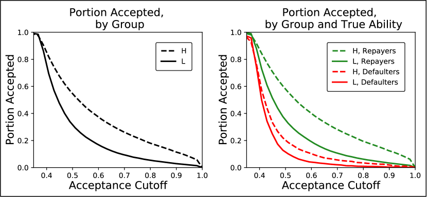
Figure 1: (a) Members of the higher-mean group are more likely to be classified as creditworthy. (b) Members of the higher-mean group are more likely to be classified as creditworthy, even when we condition on true ability. While the predictions are group-blind and there was no disparate treatment, there is disparate impact.

We demonstrate this task on real financial data from the Survey of Income and Program Participation (SIPP), defining the outcome of interest as successfully paying rent, mortgage, and utilities in every month of 2014 [U.S. Census Bureau, 2014]. We estimate the probability of successful payment for each adult in the dataset using logistic regression on three predictors: total assets, total debt, and monthly income. The lender could then translate these predicted probabilities into loan approvals and rejections at any cutoff of their choosing.

Figure 1 depicts loan access by group, given all possible cutoffs on the horizontal axis. In the left panel, we see that less-educated individuals are less likely to be classified as creditworthy at all cutoffs. This fact alone does not necessarily strike us as unfair, since it could reflect that the predictions have identified legitimate differences in repayment abilities across educational groups. However, in the right panel, we show that less-educated individuals are also less likely to be classified as creditworthy even when we condition on their eventual repayment outcome. That is, they have lower true and false positive rates than high-educated applicants. In practice, this means that a decision-maker guided by these predictions would be more likely to grant a loan to a creditworthy $H$ applicant than a creditworthy $L$ applicant, and also more likely to grant a loan to a non-creditworthy $H$ applicant than a non-creditworthy $L$ applicant.

As we will prove in Section 3, the disparate impact identified here arises when group affiliation is correlated with variables included in the prediction model. It regularly emerges in practice because we can often trace the disadvantage of disadvantaged groups through a multitude of variables, including those that are essential to predicting the outcomes we care about.

3 Characterizing the disparate impact of uncertainty

3.1 Results based on minimal assumptions

This section characterizes how uncertainty generates disparate impacts in settings where applicants are screened for opportunities. We begin with the usual observation that uncertainty affects predictions of applicant ability via regression toward the mean. The key insight is that the effect varies by group when the data guiding predictions is correlated with group membership. The probability of correctly identifying qualified applicants varies by group as a consequence. We formally define this “disparate impact of uncertainty” and identify necessary conditions to resolve it.

Consider applicants each with ability $A$. The applicants belong to groups $G\ \in\{L,H\}$ that differ in average ability, so that $\mu_{L}<\mu_{H}$ where $\mu_{G}\equiv\mathbb{{E}}[A|G]$. A decision-maker seeks to estimate $A$ using available applicant data $X$. At no point does the decision-maker observe protected group membership $G$. However, the data $X$ may be correlated with group membership. The decision-maker estimates the conditional expectation function (CEF) $\mathbb{E}[A|X]$ in the model

$$A=\mathbb{E}[A|X]+\varepsilon,$$ (1)

where $\varepsilon$ is a residual that is uncorrelated with any function of $X$, and $\mathbb{E}[A|X]$ yields the best predictions given the available data.

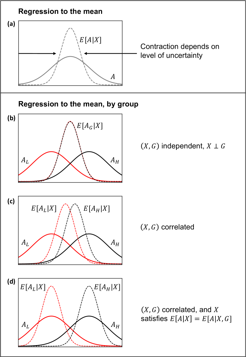
Figure 2: (a) Regression toward the mean centers predictions $\mathbb{E}[A|X]$ at the mean of ability $A$, with smaller variance. Separately considering predictions by group, however, reveals that the effect of regression toward the mean depends on the correlation between $(X,G)$. (b) If $X\perp G$, the predictions have the same distribution. (c) If $(X,G)$ are correlated, then the mean predictions will differ by group. (d) Furthermore, if $X$ actually explains the relationship between $(A,G)$, so that $\mathbb{E}[A|X]=\mathbb{E}[A|X,G]$, then predictions are centered at group-specific means. Note that the figure depicts normal distributions for simplicity, but no normality assumption is required for any result in Section 3.1.

First, note that the predictions given by the CEF follow regression toward the mean, since they are centered at the mean ability $\mathbb{E}[A]$, with variance smaller than $\operatorname{Var}[A]$. This contraction toward mean ability is depicted in Figure 2(a). As a result of the contraction, high-ability individuals are expected to have above-average predictions, but not as high as their true ability. Similarly, low-ability individuals are expected to have below-average predictions, but not as low as their true ability. The magnitude of the contraction toward the mean depends on how well $X$ describes variation in $A$: the CEF is more concentrated at the mean in high-uncertainty settings where $X$ weakly relates to $A$.

We can now explain how uncertainty impacts applicants differently by group: The contractions experienced by the groups vary systematically depending on the relationship between $G$ and the underlying data $X$. We depict three examples in Figure 2. If $X$ and $G$ are independent, the predictions follow the same distribution across groups as seen in panel (b). If $X$ and $G$ are not independent, however, then the predictions will be distributed as contractions toward group-dependent means. This is formally shown in the next proposition. When $X$ partly explains groups’ variation in ability, so that group $L$ has a relatively greater density of applicants with $X$s associated with lower ability, then the $L$ predictions will have a lower mean. Furthermore, if $X$ fully explains the groups’ variation in ability, then the best predictions will be centered exactly at the group-specific averages of ability. The partial and full cases are illustrated in panels (c) and (d) respectively.

Proposition 1.

Consider the distribution of the best predictions $\mathbb{E}[A|X]$ for group $G=g$. Its variance is smaller than the variance of ability for $g$ and its mean depends on the joint distribution of $(A,X,G)$. If $X$ fully explains the relationship between $A$ and $G$, so that $\mathbb{E}[A|X]=\mathbb{E}[A|X,G]$, then the mean is exactly equal to $\mu_{g}$.

Proof.

The variance of the best predictions for $g$ is bounded by the variance of ability, since $\operatorname{Var}[\mathbb{E}[A|X]|G=g]\leq\operatorname{Var}[\mathbb{E}[A|X]+\varepsilon|G=g]=\operatorname{Var}[A|G=g]$, where the equality follows from (1).

The mean of the best predictions for $g$ is an average over $\mathbb{E}[A|X]$ weighted by the density of $X$ given $g$. In particular, if we denote $n$ as the dimensionality of $X$ and $f_{X|G}(\bm{x}|g)$ as the conditional density of $X$ given $G=g$, then $\mathbb{E}[\mathbb{E}[A|X]|G=g]=\int_{\mathbb{R}^{n}}\mathbb{E}[A|X=\bm{x}]f_{X|G}(\bm{x}|g)d^{n}\bm{x}.$ The mean is smaller when $g$ has a greater density of $X$s associated with low $A$.

We can compute the mean in closed form if $\mathbb{E}[A|X]=\mathbb{E}[A|X,G]$. By first applying mean independence and then applying the tower property of conditional expectation, we have $\mathbb{E}[\mathbb{E}[A|X]|G=g]=\mathbb{E}[\mathbb{E}[A|X,G]|G=g]=\mathbb{E}[A|G=g]\equiv\mu_{g}$, so the distribution of the best predictions for $g$ is centered at the mean ability of applicants in $g$. ∎

To summarize, uncertainty impacts predictions differently by group. First, predictions of applicants in lower-mean groups will have lower means so long as $X$ contains variables that explain at least some of the variation in $A$ across groups. Then, uncertainty contracts predictions for each group closer to those group-specific means. Overall, predictions of applicants from groups with lower-ability distributions contract toward lower values, whereas those with higher-ability distributions contract toward higher values. We can generally expect that the presence of uncertainty causes two applicants — with equal true ability but from different groups — to vary in their predicted ability.

Decision-makers who use predictions to identify which applicants to accept and reject can then inadvertently generate disparate impacts. To see this, suppose a decision-maker wishes to identify applicants that are qualified for an opportunity. Let $Y\in\{0,1\}$ denote whether an applicant is actually qualified, and suppose qualification rates are lower in $L$ than in $H$, with $0<\mu_{L}<\mu_{H}<1$ where $\mu_{G}=\mathbb{P}[Y=1|G]$. Denote $\hat{y}\in\{0,1\}$ as the decision-maker’s binary choice to reject or accept the applicant. The “disparate impact of uncertainty” is said to arise if qualified members of $L$ are rejected at higher rates than qualified members of $H$.

Definition 1.

The disparate impact of uncertainty is present when $\text{FNR}_{L}>\text{FNR}_{H}$, where $\text{FNR}_{G}$ is the group-specific false negative rate $\mathbb{P}[\hat{y}=0|Y=1,G]$. This is mathematically equivalent to $\text{TPR}_{L}<\text{TPR}_{H}$, where $\text{TPR}_{G}$ is the group-specific true positive rate $\mathbb{P}[\hat{y}=1|Y=1,G]$.

The following lemma guarantees that $\hat{y}$ will always exhibit the disparate impact of uncertainty unless it assigns classifications to $L$ members that are systematically i) more favorable or ii) more accurate. A proof sketch is included, and interested readers are referred to a detailed proof in the appendix.

Lemma 1.

$\hat{y}$ exhibits the disparate impact of uncertainty if

• it does not over-represent members of $L$ among positive classifications:

  $$\mathbb{P}[G=L|\hat{y}=1]\leq\mathbb{P}[G=L|Y=1],$$

• and its positive or negative predictions for members of $L$ are less accurate than those of $H$:

  $$\text{PPV}_{L}<\text{PPV}_{H}\text{ or }\text{NPV}_{L}\leq\text{NPV}_{H},$$

  where $\text{PPV}_{G}\equiv\mathbb{P}[Y=1|\hat{y}=1,G]$ and $\text{NPV}_{G}\equiv\mathbb{P}[Y=0|\hat{y}=0,G]$ are the group-specific positive and negative predictive values.

Proof Sketch.

Let $\hat{\mu}_{G}$ denote the group-specific positive selection rate, $\mathbb{P}[\hat{y}=1|G]$. If (i) holds, then

$$\frac{\mu_{H}}{\mu_{L}}\leq\frac{\hat{\mu}_{H}}{\hat{\mu}_{L}}.$$ (2)

Suppose (ii) also holds, separately considering the cases $\text{PPV}_{L}<\text{PPV}_{H}$ and $\text{NPV}_{L}\leq\text{NPV}_{H}$.

Case 1: Rewriting (2) gives $\frac{\hat{\mu}_{L}}{\mu_{L}}\leq\frac{\hat{\mu}_{H}}{\mu_{H}}$, and combining with $\text{PPV}_{L}<\text{PPV}_{H}$, we get

$$\text{PPV}_{L}\frac{\hat{\mu}_{L}}{\mu_{L}}<\text{PPV}_{H}\frac{\hat{\mu}_{H}}{\mu_{H}}.$$

This is $\text{TPR}_{L}<\text{TPR}_{H}$ rewritten with Bayes’ rule.

Case 2: Note that (2) implies $\hat{\mu}_{L}<\hat{\mu}_{H}$, since $\mu_{L}<\mu_{H}$. Combining with $\text{NPV}_{L}\leq\text{NPV}_{H}$,

$$(1-\text{NPV}_{L})\frac{1-\hat{\mu}_{L}}{\mu_{L}}>(1-\text{NPV}_{H})\frac{1-\hat{\mu}_{H}}{\mu_{H}}.$$

This is $\text{FNR}_{L}>\text{FNR}_{H}$ rewritten with Bayes’ rule, where $\text{FNR}_{G}$ is the group-specific false negative rate $\mathbb{P}[\hat{y}=0|Y=1,G]$. Because false negative and true positive rates are related by $\text{FNR}=1-\text{TPR}$, we have $1-\text{TPR}_{L}>1-\text{TPR}_{H}\implies\text{TPR}_{L}<\text{TPR}_{H}$. ∎

The contrapositive gives necessary conditions to eliminate the disparate impact of uncertainty:

Theorem 1.

If $\hat{y}$ does not exhibit the disparate impact of uncertainty, then it must over-represent members of $L$ among positive classifications or predict their outcomes more accurately:

• $\mathbb{P}[G=L|\hat{y}=1]>\mathbb{P}[G=L|Y=1]$, or

• $\text{PPV}_{L}\geq\text{PPV}_{H}\text{ and }\text{NPV}_{L}>\text{NPV}_{H}$.

Lemma 1 and Theorem 1 hold in general, as they are founded only on the assumptions that qualification rates differ across groups and that there is predictive uncertainty. We have remained agnostic as to how the decision-maker has formulated her decisions $\hat{y}$. Therefore, Theorem 1 provides practical guidance across a wide range of settings. It establishes that there are only two possible solutions to overcome the disparate impact of uncertainty in practice: The decision-maker can i) design prediction schemes that over-select members of a group with lower qualification rates, such as by setting more lenient admission criteria for members of that group. Alternatively, she can ii) increase the accuracy of predictions for this group, such as by investing in additional data acquisition.

3.2 A generalized model of statistical discrimination

In this section, we introduce additional assumptions in the form of a stylized model to show how the disparate impact of uncertainty emerges from a generalization of statistical discrimination. These results expand the canonical insights of Aigner and Cain [1977] to settings where decision-makers screen applicants based on an arbitrary set of variables, rather than on an unbiased test score and a demographic variable. In this generalization, the disparate impact discovered by Aigner and Cain [1977] can emerge even when decision-makers are barred from using demographic variables. We show the disparate impact can be eliminated by increasing the explanatory power of the predictors for the affected group.

Suppose an accuracy-maximizing lender uses data $X$ to predict repayment ability $A$. For this model, assume that $X$ explains variation in $A$ across demographic groups $G$ so that $\mathbb{E}[A|X]=\mathbb{E}[A|X,G]$. This holds trivially if $G\in X$. But it could also hold if $X$ contains financial data that explain the lower repayment rates of the disadvantaged group.

As in Eq. (1) from the previous section, applicant ability $A$ can be decomposed into a signal that is explained by the data $X$ and a residual that is unexplained by $X$. We can write this decomposition for group $G=g$ as

$$A_{g}=S_{g}+\varepsilon_{g},\\$$ (3)

where the signal $S_{g}\equiv\mathbb{E}[A_{g}|X_{g}]$ is the most accurate prediction of ability given the data.

Suppose that the lender observes $S_{g}$ and accepts all applicants that have $S_{g}$ above a cutoff of her choosing. The choice of cutoff depends on her relative valuation of false positive and false negative classifications. In a setting where false negatives are more costly, the cutoff will be lower, and in a setting where false positives are more costly, the cutoff will be higher. We call low-cutoff settings “lemon-dropping markets” and high-cutoff settings “cherry-picking markets,” as in Bartoš et al. [2016].

For model tractability, we assume as in Aigner and Cain [1977] that $S_{g}$ and $\varepsilon_{g}$ are bivariate normal. Our model is therefore specified by signals $S_{g}\sim\mathcal{N}(\mu_{g},\sigma^{2}_{S_{g}})$, residuals $\varepsilon_{g}\sim\mathcal{N}(0,\sigma^{2}_{\varepsilon_{g}})$, and ability $A_{G}\sim\mathcal{N}(\mu_{g},\sigma^{2}_{S_{g}}+\sigma^{2}_{\varepsilon_{g}})$. We can use the bivariate normal distribution assumption to calculate the expected signal for a member of group $g$ with ability $a$. Derived in the appendix, it is

$$\mathbb{E}[S_{g}|A_{g}=a]=(1-\gamma_{g})\mu_{g}+\gamma_{g}a\text{, where }\gamma_{g}\equiv\frac{\sigma_{S_{g}}^{2}}{\sigma_{S_{g}}^{2}+\sigma_{\varepsilon_{g}}^{2}}.$$ (4)

Therefore, the expected signal is a weighted average of the true ability and the group mean. The weight $\gamma_{g}$ on the true ability reflects the portion of $A_{g}$’s total variance that is captured by the observable signals $S_{g}$, and the weight $1-\gamma_{g}$ on the mean reflects the unexplained variance due to the presence of uncertainty. As $\gamma_{g}$ increases, the signal is expected to closely track true ability. As $\gamma_{g}$ decreases, however, the signals are expected to bunch more tightly about the group mean.

An immediate consequence is that an individual from a lower-mean group $L$ with true ability $a$ can generally be expected to have a different predicted ability than an individual from a higher-mean group $H$ with the same ability $a$.

We next consider two cases, one demonstrating the disparate impact of uncertainty and the second correcting it. The first case equates the observed variance in ability ($\gamma_{L}=\gamma_{H}$), while the second explores the effect of increasing the observed variance for the $L$ group ($\gamma_{L}>\gamma_{H}$). In each case, the best estimate of ability for each group is given by the signal. However, in the latter case, the estimate is made more precise for $L$.

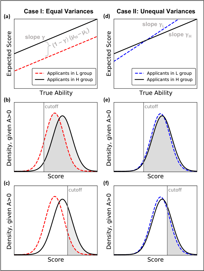
Figure 3: Plots in left column illustrate the case with equal variance signals, and plots in right column are based on higher-variance signals for the $L$ group. In (a), we see that expected signals conditional on true underlying ability are systematically higher for $H$ members. In (b) and (c), we plot the distribution of signals for qualified applicants ($A>0$) in a lemon-dropping and cherry-picking market, respectively. The group-specific true positive rates are given by the portion under each curve that is shaded. Members of $H$ have higher true positive rates, and the difference is particularly stark in the cherry-picking example. The imbalance is alleviated when the $L$ signals become more informative, as seen in (d)-(f).

3.2.1 Equally informative signal

First consider a setting with $\gamma^{L}=\gamma^{H}\equiv\gamma$. We depict expected signals conditional on true underlying ability in Figure 3(a). For each level of ability, individuals in the $H$ group are expected to have higher observable signals. The gap between their expected signals and those of the $L$ group is seen to increase in the differences between their means $(\mu_{H}-\mu_{L})$ and the extent of the uncertainty, $(1-\gamma)$.

Since the lender applies the same cutoff rule to all applicants, the systematic disparities in signals propagate into systematic disparities in the ultimate acceptance decisions. We formally show this by defining applicants’ true qualification $Y=\mathbbm{1}\{A>0\}$ and deriving the conditional distribution of $S$ given $Y$. In Figure 3(b) and 3(c) we illustrate the distributions of signals of qualified individuals, given two examples of lender cutoffs. Because the true positive rate is the portion of qualified individuals ultimately granted a loan, it is straightforward to visualize it on the plot: each group’s true positive rate is given by the portion of the area under its curve that is shaded, corresponding to those applicants with a signal above the cutoff. We observe that the true positive rates are higher for the $H$ group in both lemon-dropping and cherry-picking markets, and that the effect is most stark when the lender cherry-picks applicants at the top of the distribution, as in Figure 3(c).

3.2.2 More informative $L$ signal

Next consider the case where the signal captures a greater portion of the variance in ability for the $L$ group than for the $H$ group, that is when $\gamma^{L}>\gamma^{H}$. Then imbalances in the true positive rate are reduced. The expected signals conditional on true underlying ability are plotted in Figure 3(d), where we see that at low levels of underlying ability, $L$ members have lower expected signals than $H$ members, whereas they have higher expected signals at higher levels of ability. Meanwhile, the distributions of the signals of qualified individuals are plotted in Figures 3(e) and 3(f). After increasing the signal variance for $L$, we see that the shaded portion under each groups’ curve is approximately the same, signifying that the groups’ true positive rates are approximately the same.

3.2.3 Connection to discrimination models

Biased measurement models

Group-blind prediction is known to underrepresent disadvantaged groups when decision-makers estimate applicant ability with implicit bias in means or with different levels of variance. Kleinberg and Raghavan [2018]; Emelianov et al. [2020] characterize these phenomena in cases where groups have the same underlying ability distributions.

By contrast, here we consider underrepresentation emerging from unbiased measurement of two groups’ differing ability distributions. We are motivated by practical cases where past disadvantage makes it harder for some applicants to succeed if they were screened in by the decision-maker. For example, members of a disadvantaged group may have relatively lower ability to perform well in college after coming from underfunded high schools, or lower ability to pay back loans due to lower access to high-paying jobs. In the corresponding decisions to admit students to college or grant applicants loans, we have shown that equal levels of predictive uncertainty across groups can lead not only to general underrepresentation of disadvantaged groups, but actually to underrepresentation of their equally-capable applicants.

Canonical statistical discrimination model

Aigner and Cain [1977] showed that when a rational decision-maker is presented with applicants’ noisy unbiased signals for ability, she then has an incentive to weigh applicants’ group membership alongside those signals to improve the accuracy of her predictions. As a result, the decision-maker will assign equal outcomes to applicants with equal expected ability across groups, but unequal outcomes for applicants with equal true ability. The result was foundational in identifying a root cause of discrimination, based not on emotion or taste, but on mathematical judgment.

Our model studies a generalized form of statistical discrimination. We consider cases where the decision-maker accesses an arbitrary set of variables $X$ to predict ability $A$, estimating a signal $S=\mathbb{E}[A|X]$ from the econometric model $A=S+\varepsilon$. We assume that $X$ explains group differences in outcomes. This is trivially satisfied if $X$ contains an unbiased test score and a demographic group identifier, in which case our model maps to Aigner and Cain [1977]. If, however, $X$ contains only non-demographic variables that explain the variation in ability across demographic groups, then the signal $S$ will still exhibit reversion to group-specific means. Therefore, the presence of variables that explain group differences in ability will replicate the same mathematical effect caused by statistical discrimination [Aigner and Cain, 1977].

As a practical matter, this model shows that while deleting demographic variables from datasets resolves the disparities in Aigner and Cain [1977], it is not a reliable remedy in general. Rather, a reliable remedy is to increase the accuracy of predictions for the affected group: data enrichment, as opposed to data omission.

4 Empirical application

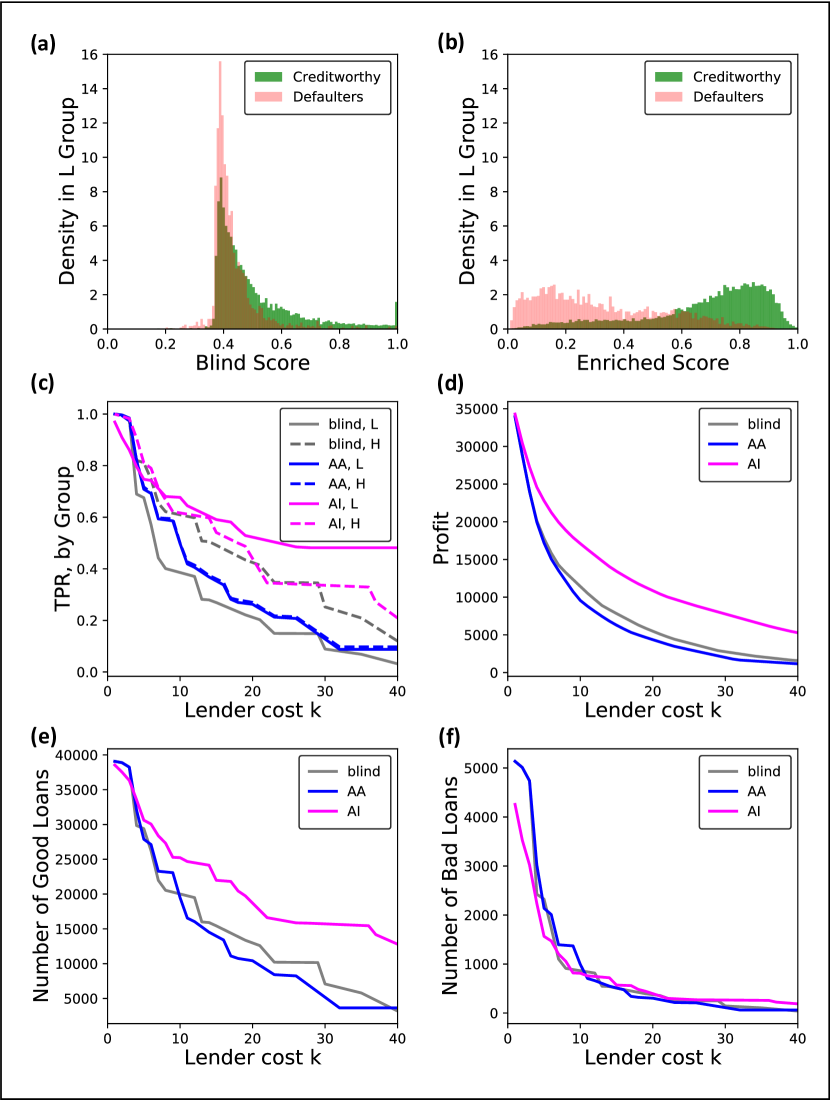
Figure 4: (a) Scores based on limited dataset are bunched at low values for creditworthy and defaulting applicants. (b) Scores based on enriched dataset, in Affirmative Information scheme, better distinguish creditworthy applicants. (c) When blind prediction (gray) is replaced by Affirmative Action (blue), the TPR of the higher-mean group falls and the TPR of the lower-mean group increases. Meanwhile, when blind prediction is replaced by Affirmative Information (pink), the TPR of the higher-mean group is roughly unchanged and the TPR of the lower-mean group increases. For all but the lowest values of $k$, Affirmative Information is associated with higher TPRs for both groups than Affirmative Action. (d) Affirmative Information corresponds to greater lender profits than both blind prediction and Affirmative Action. (e) Affirmative Action tends to reduce the total number of good loans administered compared to blind prediction, whereas Affirmative Information increases that number beyond the levels in both alternative schemes. (f) All three schemes yield similar numbers of bad loans administered.

We now return to our empirical example from Section 2, where we demonstrated how a set of credit risk scores can lead to disparate outcomes across education groups. Despite the fact that the scores were constructed without group identifiers or sensitive predictors, they yielded lower true and false positive rates to less-educated applicants at every cutoff. Here, we contrast traditional group-blind prediction with two strategies for increasing positive classifications of the creditworthy individuals among them: Affirmative Action and Affirmative Information. Affirmative Action works by adjusting the disadvantaged group’s criteria for acceptance, while Affirmative Information works by adding data to enhance the accuracy of the disadvantaged group’s predictions.

As before, we use SIPP, a nationally-representative panel survey of the civilian population [U.S. Census Bureau, 2014]. We label our outcome of “creditworthiness” as the successful payment of rent, mortgage, and utilities in every month of 2014. Of the overall sample, we call the 55% who studied beyond a high school education group $H$ and those with at most a high school education group $L$.

We suppose a lender is using repayment predictions to assign loan denials and approvals, without observing individuals’ group membership. The lender approves loans for anyone whose score corresponds to a positive expected return, and therefore imposes a cutoff rule that depends on the relative cost of false positive and false negative errors. To model the lender choice, we consider a profit function that generates cutoff decision rules: $\text{TP}-k\text{FP}$, where TP is the number of creditworthy applicants given loans, FP is the number of defaulters given loans, and $k$ is a constant representing the relative cost of false positive classifications. We compute the lender’s classification choices by iteratively considering different possible values of $k$ in the profit function, and determining at each $k$ what would be the lender’s endogenously chosen classification decisions.

The lender first formulates group-blind predictions of repayment ability using a logistic regression on total assets, debt, and income. In the blind scheme, they select a single profit-maximizing cutoff without regard to group membership. In an Affirmative Action scheme, meanwhile, they choose an accuracy-maximizing pair of group-dependent cutoffs among the set that generates equal TPRs among $L$ and $H$ applicants. Lastly, in the Affirmative Information scheme, we suppose the decision-maker has taken effort to gather additional data about the $L$ applicants, and to simulate that we train new scores for $L$ applicants using the much richer set of variables available in SIPP, spanning more detailed household financials as well as sensitive characteristics such as food security, family structure, and participation in social programs. The lender then makes profit-maximizing acceptance decisions based off the original $H$ scores and the enriched $L$ scores. To summarize the difference between the schemes, Affirmative Action works by enforcing more lenient cutoffs for applicants in $L$, while Affirmative Information works by enhancing the accuracy of $L$ scores. The distribution of $L$ scores used in the Affirmative Action scheme are depicted in Figure 4(a) while those used in the Affirmative Information scheme are depicted in (b).

In Figure 4(c), we plot creditworthy applicants’ access to positive classifications given different values of lender cost $k$. The gray lines show that blind prediction yields consistently higher TPRs for members of $H$ compared to $L$, as in Section 2. The Affirmative Action intervention is depicted in blue and the Affirmative Information intervention in pink. We see that Affirmative Action eliminates the disparity generated by blind prediction, but does not push the TPR for $L$ all the way to the original levels of the $H$ applicants. Rather, the added cost to the lender of reducing disparities leads them to set cutoffs that cause the two groups’ TPRs to meet in the middle, raising the TPR of $L$ while also reducing that of $H$. By comparison, Affirmative Information is associated with leaving the original TPR for $H$ essentially unchanged, while significantly raising the TPR for $L$ beyond its level in blind prediction or Affirmative Action for all but the smallest values of $k$. Compared to Affirmative Action, it yields greater access to positive classifications for both groups’ creditworthy applicants.

Figure 4(d) illustrates the impact on lender profit from each intervention. For many values of $k$, Affirmative Action reduces profit. Yet for all values of $k$, Affirmative Information increases profit. In Figure 4(e) and (f), we see the effect works through increasing the overall number of repaid loans, while leaving the overall number of defaults essentially unchanged.

There are two noteworthy caveats to Affirmative Information. The first is that Affirmative Information requires data acquisition, which is costly and will reduce profits below the level seen in Figure 4(d). The second is that it may be less effective in lemon-dropping settings in which cutoffs are well below the mean, as seen in Figure 4(c) at the lowest values of $k$.

Overall, this empirical example has demonstrated the potential advantages of Affirmative Information as a tool to broaden access to opportunity. Particularly in settings with selective admissions criteria, employing Affirmative Information rather than Affirmative Action can yield TPRs that are higher for both groups. In addition, depending on the cost of the data acquisition, Affirmative Information may benefit decision-makers as well. Targeted data enrichment can therefore create natural incentives to broaden access to opportunities.

5 Conclusion

This paper has shown that even facially neutral prediction models can create systematic disparities in access to opportunity. Even if the models omit variables tracking demographic characteristics and their proxies, uncertainty causes them to assign different probabilities of acceptance to equally-qualified applicants in groups with differing mean ability. This effect, which we have called the disparate impact of uncertainty, can arise in all settings where decision-makers screen applicants who come from demographic groups with different risk distributions: it can thus compromise fair judgment in lending, bail decisions, college admissions, hiring, medical treatment assignments, and foster care placements, to name a few examples.

We hope that our work will motivate decision-makers to consider shifting their antidiscrimination efforts from traditional data omission to thoughtful data enrichment. While traditional analyses of fair prediction implicitly treat the available data as fixed, we explored how relaxing that constraint and permitting data acquisition expands the frontier of possible prediction to achieve outcomes that are both more efficient and more equitable.

Now that the Supreme Court has struck down Affirmative Action, Affirmative Information may serve as an effective alternative to expand access to opportunity while supporting competing notions of fairness. At least two roads lie ahead. First is statistical guidance for private actors on how they can pinpoint which data would best identify qualified individuals if they were to gather it. Second is how the public, through economic incentives and the law, can enable private actors to invest in data acquisition.

References

- [1]
- Aigner and Cain [1977] Aigner, Dennis J, and Glen G Cain. 1977. “Statistical theories of discrimination in labor markets.” Ilr Review, 30(2): 175–187.
- Angrist and Pischke [2008] Angrist, Joshua D., and Jörn-Steffen Pischke. 2008. Mostly Harmless Econometrics: An Empiricist’s Companion. Princeton University Press.
- Angwin et al. [2016] Angwin, Julia, Jeff Larson, Surya Mattu, and Lauren Kirchner. 2016. “Machine bias.” ProPublica, May, 23: 2016.
- Arnold, Dobbie and Hull [2022] Arnold, David, Will Dobbie, and Peter Hull. 2022. “Measuring racial discrimination in bail decisions.” American Economic Review, 112(9): 2992–3038.
- Bartoš et al. [2016] Bartoš, Vojtěch, Michal Bauer, Julie Chytilová, and Filip Matějka. 2016. “Attention discrimination: Theory and field experiments with monitoring information acquisition.” American Economic Review, 106(6): 1437–75.
- Chen, Johansson and Sontag [2018] Chen, Irene, Fredrik D Johansson, and David Sontag. 2018. “Why is my classifier discriminatory?” 3539–3550.
- Dwork et al. [2012] Dwork, Cynthia, Moritz Hardt, Toniann Pitassi, Omer Reingold, and Richard Zemel. 2012. “Fairness through awareness.” 214–226.
- Dwork et al. [2018] Dwork, Cynthia, Nicole Immorlica, Adam Tauman Kalai, and Max Leiserson. 2018. “Decoupled classifiers for group-fair and efficient machine learning.” 119–133.
- Emelianov et al. [2020] Emelianov, Vitalii, Nicolas Gast, Krishna P. Gummadi, and Patrick Loiseau. 2020. “On Fair Selection in the Presence of Implicit Variance.” ACM.
- Eubanks [2018] Eubanks, Virginia. 2018. “A child abuse prediction model fails poor families.” Wired Magazine.
- Hardt, Price and Srebro [2016] Hardt, Moritz, Eric Price, and Nati Srebro. 2016. “Equality of opportunity in supervised learning.” 3315–3323.
- Kleinberg and Raghavan [2018] Kleinberg, Jon, and Manish Raghavan. 2018. “Selection Problems in the Presence of Implicit Bias.” Vol. 94 of Leibniz International Proceedings in Informatics (LIPIcs), 33:1–33:17. Dagstuhl, Germany:Schloss Dagstuhl–Leibniz-Zentrum fuer Informatik.
- Kleinberg and Mullainathan [2019] Kleinberg, Jon, and Sendhil Mullainathan. 2019. “Simplicity Creates Inequity: Implications for Fairness, Stereotypes, and Interpretability.” EC ’19, 807–808. New York, NY, USA:Association for Computing Machinery.
- Kleinberg et al. [2018] Kleinberg, Jon, Jens Ludwig, Sendhil Mullainathan, and Ashesh Rambachan. 2018. “Algorithmic fairness.” Vol. 108, 22–27.
- Lazar Reich and Vijaykumar [2021] Lazar Reich, Claire, and Suhas Vijaykumar. 2021. “A Possibility in Algorithmic Fairness: Can Calibration and Equal Error Rates Be Reconciled?”
- Obermeyer et al. [2019] Obermeyer, Ziad, Brian Powers, Christine Vogeli, and Sendhil Mullainathan. 2019. “Dissecting racial bias in an algorithm used to manage the health of populations.” Science, 366(6464): 447–453.
- Rambachan et al. [2020] Rambachan, Ashesh, Jon Kleinberg, Sendhil Mullainathan, and Jens Ludwig. 2020. “An economic approach to regulating algorithms.” National Bureau of Economic Research.
- U.S. Census Bureau [2014] U.S. Census Bureau. 2014. “Survey of Income and Program Participation, Panel Wave 2.” United States Department of Commerce. https://www.census.gov/programs-surveys/sipp/data/datasets.html (accessed: January 17, 2020).