Social Network Analysis: From Graph Theory to Applications with Python

Abstract.

Social network analysis is the process of investigating social structures through the use of networks and graph theory. It combines a variety of techniques for analyzing the structure of social networks as well as theories that aim at explaining the underlying dynamics and patterns observed in these structures. It is an inherently interdisciplinary field which originally emerged from the fields of social psychology, statistics and graph theory. This talk will covers the theory of social network analysis, with a short introduction to graph theory and information spread. Then we will deep dive into Python code with NetworkX to get a better understanding of the network components, followed-up by constructing and implying social networks from real Pandas and textual datasets. Finally we will go over code examples of practical use-cases such as visualization with matplotlib, social-centrality analysis and influence maximization for information spread.

1. Introduction

Social network analysis is the process of investigating social structures through the use of networks and graph theory. This article introduces data scientists to the theory of social networks, with a short introduction to graph theory, information spread and influence maximization (Goldenberg et al., 2018). It dives into Python code with NetworkX (Hagberg et al., 2008) constructing and implying social networks from real datasets. A video version of this article is available on Pycon Youtube channel.

Figure 1. Example network and components

2. Network Theory

2.1. Network Components

We’ll start with a brief intro in network’s basic components: nodes and edges.

Nodes (A,B,C,D,E in the example) are usually representing entities in the network, and can hold self-properties (such as weight, size, position and any other attribute) and network-based properties (such as Degree- number of neighbours or Cluster- a connected component the node belongs to etc.).

Edges represent the connections between the nodes, and might hold properties as well (such as weight representing the strength of the connection, direction in case of asymmetric relation or time if applicable).

These two basic elements can describe multiple phenomena, such as social connections, virtual routing network, physical electricity networks, roads network, biology relations network and many other relationships.

2.2. Real-world networks

Real-world networks and in particular social networks have a unique structure which often differs them from random mathematical networks. Figure 2 provides examples of complex networks (taken from (Huang et al., 2005)).

Figure 2. Complex networks (taken from (Huang et al., 2005))

• Small World phenomenon (Kleinberg, 2000) claims that real networks often have very short paths (in terms of number of hops) between any connected network members. This applies for real and virtual social networks (the six handshakes theory) and for physical networks such as airports or electricity of web-traffic routing.

• Scale Free (Barabási et al., 2000) networks with power-law degree distribution have a skewed population with a few highly-connected nodes (such as social-influences) and a lot of loosely-connected nodes.

• Homophily (McPherson et al., 2001) is the tendency of individuals to associate and bond with similar others, which results in similar properties among neighbors.

2.3. Centrality Measures

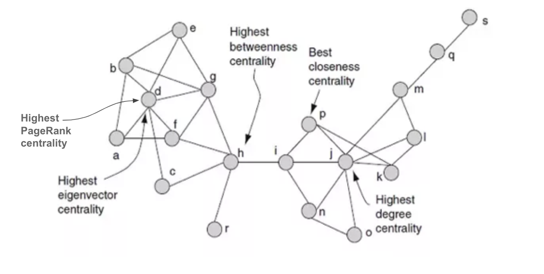
Figure 3. Illustration of various centrality measures (taken from (Ortiz-Arroyo, 2010)).

Highly central nodes play a key role of a network, serving as hubs for different network dynamics. However the definition and importance of centrality might differ from case to case, and may refer to different centrality measures, as depicted in figure 3 (taken from (Ortiz-Arroyo, 2010)).

• Degree — the amount of neighbors of the node

• EigenVector (Bonacich, 2007) / PageRank (Page et al., 1999) — iterative circles of neighbors

• Closeness (Okamoto et al., 2008) — the level of closeness to all of the nodes

• Betweenness (Brandes, 2001) — the amount of short path going through the node

Different measures can be useful in different scenarios such web-ranking (page-rank), critical points detection (betweenness), transportation hubs (closeness) and other applications.

3. Building a Network

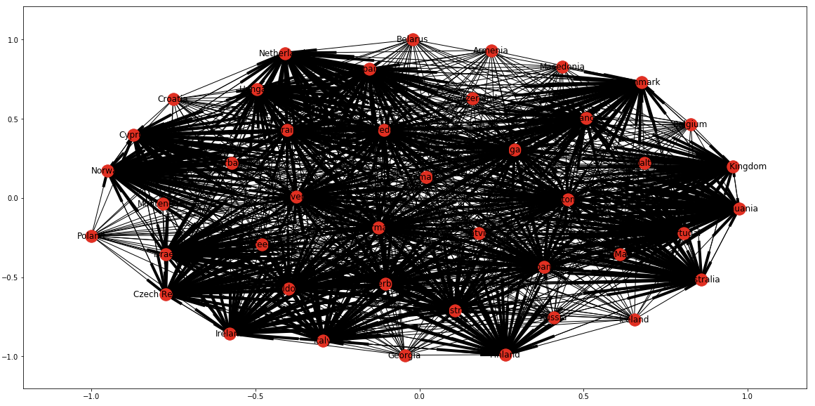
Figure 4. nx.draw_networkx(G) outcome on Eurovision 2018 votes network

Networks can be constructed from various datasets, as long as we’re able to describe the relations between nodes. In the following example we’ll build and visualize the Eurovision 2018 votes network (based on official data) with Python networkx (Hagberg et al., 2008) package. We’ll read the data from excel file to a pandas dataframe to get a tabular representation of the votes. Since each row represents all of the votes of each country, we’ll melt the dataset to make sure that each row represents a single vote (edge) between two countries (nodes). Then, we will build a directed graph using networkx from the edgelist we have as a pandas dataframe. Finally, we’ll try the generic method to visualize, as shown in code 1 (full code can be found at Github repository)

Listing 1: Creating a network with Networkx

⬇

votes_data = pd.read_excel(’data.xlsx’)

votes_melted = votes_data.melt(

[’Rank’,’Running␣order’, ’Country’,’Total’],

var_name = ’Source␣Country’,value_name=’points’)

G = nx.from_pandas_edgelist(votes_melted, source=’Source␣Country’,

target=’Country’, edge_attr=’points’, create_using=nx.DiGraph())

nx.draw_networkx(G)

3.1. Visualization

Unfortunately the built-in draw method results in a very incomprehensible figure as shown in figure 4. The method tries to plot a highly connected graph, but with no useful “hints” it’s unable to make a lot of sense from the data. We will enhance the figure by dividing and conquering different visual aspects of the plot with a prior knowledge that we have about the entities:

• Position — each country is assigned according to its geo-position

• Style — each country is recognized by its flag and flag colors

• Size — the size of nodes and edges represents the amount of points

Plotting of the network components in parts is shown in code 2.

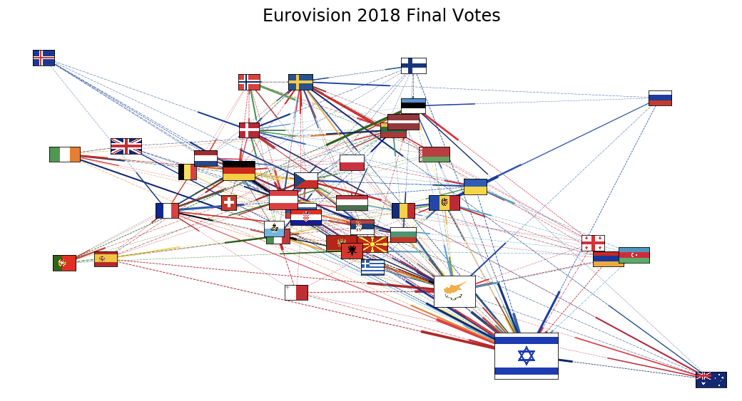
Figure 5. Step-by-step Eurovision network plot

Listing 2: Network components plotting

⬇

for e in G.edges(data=True):

width = e[2][’points’]/24

style=styles[int(width*3)]

nx.draw_networkx_edges(G,pos, edgelist=[e],width=width, style=style,

edge_color = RGB(*flag_color[e[0]] )

for node in G.nodes():

imsize = G.in_degree(node, weight=’points’)

flag = mpl.image.imread(flags[node])

(x,y) = pos[node]

xx,yy = trans((x,y))

xa,ya = trans2((xx,yy))

country = plt.axes( [xa-imsize/2.0, ya-imsize/2.0, imsize, imsize ])

country.imshow(flag)

country.set_aspect(’equal’)

country.tick_params(**tick_params)

The new figure 5 is a bit more readable, and giving us a brief overview of the votes. As a general side-note, plotting networks is often hard and requires to perform thoughtful tradeoffs between the amount of data presented and the communicated message. (You can try to explore other network visualization tools such as Gephi , Pyvis or GraphChi).

4. Information Flow

Information diffusion (Shakarian et al., 2015) process may resemble a viral spread of a disease, following contagious dynamics of hopping from one individual to his social neighbors. Two popular basic models are often used to describe the process:

Linear Threshold (Shakarian et al., 2013) defines a threshold-based behavior, where the influence accumulates from multiple neighbors of the node, which becomes activated only if the cumulative influence passed a certain threshold according to the following formula:

$$\sum_{active_{u}}W_{uv}\geq\theta_{v}$$

Such behavior is typical to movie recommendations, where a tip from of one of your friends might eventually convince you to see a movie, after hearing a lot about it.

In the Independent Cascade model (Goldenberg et al., 2001), each of the node’s active neighbors has a probabilistic and independent chance to activate the node. This resembles a viral virus spread, such as in Covid-19, where each of the social interactions might trigger the infection.

4.1. Information Flow Example

To illustrate an information diffusion process we’ll use the Storm of Swords network, based on Game of Thrones show characters. The network was constructed based on co-appearance in the “Song of Ice and Fire books” (Beveridge and Shan, 2016).

Relying on the independent cascade model, we’ll try to track down rumor spreading dynamics, which are quite common in this show. Suppose Jon Snow knows nothing at the beginning of the process, while his two loyal friends, Bran Stark and Samwell Tarly, know a very important secret about his life. Let’s watch how the rumor spreads under the Independent Cascade model:

Listing 3: Independent Cascade Code

⬇

def ind_cascade(G,t,infection_times):

max_w = max([e[2][’weight’] for e in G.edges(data=True)])

current_infectious = [n for n in infection_times

if infection_times[n]==t]

for n in current_infectious:

for v in G.neighbors(n):

if v not in infection_times:

if G.get_edge_data(n,v)[’weight’]>=np.random.random()*max_w:

infection_times[v] = t+1

return infection_times

inf_times = {’Bran-Stark’:-1, ’Samwell-Tarly’:-1,’Jon-Snow’:0}

for t in range(10):

plot_G(subG,pos,infection_times,t)

inf_times=ind_cascade(subG,t,inf_times)

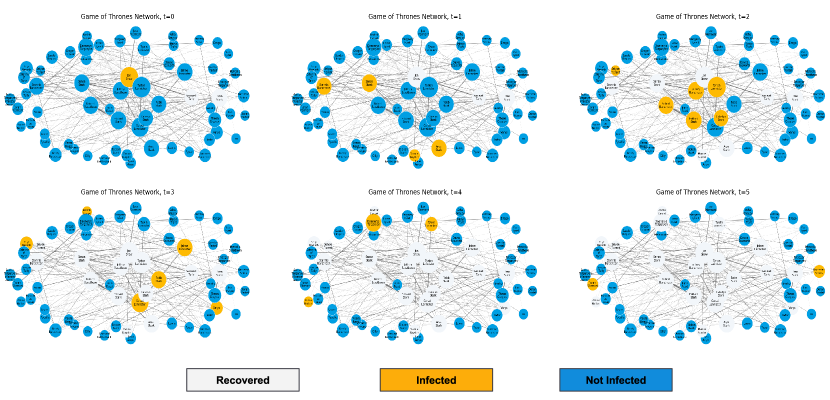
Figure 6. Independent Cascade diffusion simulation on Game of Thrones network

As shown in figure 6 the rumor reaches Jon at t=1, spreads to his neighbors in the following time-steps and quickly spreads all around the network, resulting in being a public knowledge. Such dynamics are highly dependent on model parameters, which can drive the diffusion process to different patterns.

5. Influence Maximization

The influence maximization problem (Kempe et al., 2003) describes a marketing (but not only) setup, where the goal of the marketer is to select a limited set of nodes in the network (seeding set) such that will naturally spread the influence to as much nodes as possible. For example, consider inviting a limited amount of influencers to a prestigious product launch event, in order to spread the word to the rest of their network. Such influencers can be identified with numerous techniques, such as using the centrality measures (Borgatti, 2005; Hinz et al., 2011) we’ve mentioned above. The most central nodes in Game of Thrones network according to different measures are listed in table 1.

Table 1. Leading characters per centrality measure

Degree		Weighted Degree		Pagerank		Betweenness
Name	Score	Name	Score	Name	Score	Name	Score
Tyrion	40	Tyrion	1842	Tyrion	0.052	Robert	0.22
Robert	37	Cersei	1627	Jon Snow	0.048	Brienne	0.12
Joffrey	35	Joffrey	1518	Cersei	0.046	Rodrik	0.11

As we can see in table 1, some of the characters re-occur at the top of different measures, and are also well known for their social influence in the show. By simulating the selection of most central nodes we observe that picking a single node of the network can achieve about 50% of network coverage — That’s how important social influencers might be.

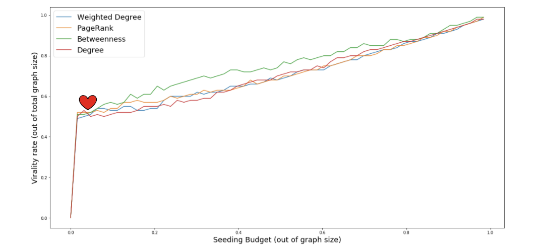
Figure 7. Network influence coverage by different methods and budgets

On the other hand Influence Maximization is Hard. In fact it’s considered as an NP-Hard problem. Many heuristics were developed to find the best seeding set in an efficient calculation. Trying a brute-force method to find the best seeding couple in our network resulted in spending 41 minutes and achieving 56% of coverage (by selecting Robert Baratheon and Khal Drogo)- a result that would be hard to achieve with centrality heuristics.

6. Conclusion

Network analysis is a complex and useful tool for various domains, in particular in the rapidly growing social networks. The applications of such analysis include marketing influence maximization, fraud detection or recommender systems. There are multiple tools and techniques that can be applied on network datasets, but they need to be chosen wisely, taking into account the problem’s and the network’s unique properties.

References

- (1)
- Barabási et al. (2000) Albert-László Barabási, Réka Albert, and Hawoong Jeong. 2000. Scale-free characteristics of random networks: the topology of the world-wide web. Physica A: statistical mechanics and its applications 281, 1 (2000), 69–77.
- Beveridge and Shan (2016) Andrew Beveridge and Jie Shan. 2016. Network of thrones. Math Horizons 23, 4 (2016), 18–22.
- Bonacich (2007) Phillip Bonacich. 2007. Some unique properties of eigenvector centrality. Social networks 29, 4 (2007), 555–564.
- Borgatti (2005) Stephen P Borgatti. 2005. Centrality and network flow. Social networks 27, 1 (2005), 55–71.
- Brandes (2001) Ulrik Brandes. 2001. A faster algorithm for betweenness centrality. Journal of mathematical sociology 25, 2 (2001), 163–177.
- Goldenberg et al. (2018) Dmitri Goldenberg, Alon Sela, and Erez Shmueli. 2018. Timing matters: Influence maximization in social networks through scheduled seeding. IEEE Transactions on Computational Social Systems 5, 3 (2018), 621–638.
- Goldenberg et al. (2001) Jacob Goldenberg, Barak Libai, and Eitan Muller. 2001. Talk of the network: A complex systems look at the underlying process of word-of-mouth. Marketing letters 12, 3 (2001), 211–223.
- Hagberg et al. (2008) Aric A. Hagberg, Daniel A. Schult, and Pieter J. Swart. 2008. Exploring Network Structure, Dynamics, and Function using NetworkX. In Proceedings of the 7th Python in Science Conference, Gaël Varoquaux, Travis Vaught, and Jarrod Millman (Eds.). Pasadena, CA USA, 11 – 15.
- Hinz et al. (2011) Oliver Hinz, Bernd Skiera, Christian Barrot, and Jan U Becker. 2011. Seeding strategies for viral marketing: An empirical comparison. Journal of Marketing 75, 6 (2011), 55–71.
- Huang et al. (2005) Chung-Yuan Huang, Chuen-Tsai Sun, and Hsun-Cheng Lin. 2005. Influence of local information on social simulations in small-world network models. Journal of Artificial Societies and Social Simulation 8, 4 (2005).
- Kempe et al. (2003) David Kempe, Jon Kleinberg, and Éva Tardos. 2003. Maximizing the spread of influence through a social network. In Proceedings of the ninth ACM SIGKDD international conference on Knowledge discovery and data mining. ACM, 137–146.
- Kleinberg (2000) Jon Kleinberg. 2000. The small-world phenomenon: An algorithmic perspective. In Proceedings of the thirty-second annual ACM symposium on Theory of computing. ACM, 163–170.
- McPherson et al. (2001) Miller McPherson, Lynn Smith-Lovin, and James M Cook. 2001. Birds of a feather: Homophily in social networks. Annual review of sociology 27, 1 (2001), 415–444.
- Okamoto et al. (2008) Kazuya Okamoto, Wei Chen, and Xiang-Yang Li. 2008. Ranking of closeness centrality for large-scale social networks. In International workshop on frontiers in algorithmics. Springer, 186–195.
- Ortiz-Arroyo (2010) Daniel Ortiz-Arroyo. 2010. Discovering sets of key players in social networks. In Computational social network analysis. Springer, 27–47.
- Page et al. (1999) Lawrence Page, Sergey Brin, Rajeev Motwani, and Terry Winograd. 1999. The PageRank citation ranking: Bringing order to the web. Technical Report. Stanford InfoLab.
- Shakarian et al. (2015) Paulo Shakarian, Abhinav Bhatnagar, Ashkan Aleali, Elham Shaabani, and Ruocheng Guo. 2015. Diffusion in social networks. Springer.
- Shakarian et al. (2013) Paulo Shakarian, Sean Eyre, and Damon Paulo. 2013. A scalable heuristic for viral marketing under the tipping model. Social Network Analysis and Mining 3, 4 (2013), 1225–1248.