Implicit Regularization in Tensor Factorization

Abstract

Recent efforts to unravel the mystery of implicit regularization in deep learning have led to a theoretical focus on matrix factorization — matrix completion via linear neural network. As a step further towards practical deep learning, we provide the first theoretical analysis of implicit regularization in tensor factorization — tensor completion via certain type of non-linear neural network. We circumvent the notorious difficulty of tensor problems by adopting a dynamical systems perspective, and characterizing the evolution induced by gradient descent. The characterization suggests a form of greedy low tensor rank search, which we rigorously prove under certain conditions, and empirically demonstrate under others. Motivated by tensor rank capturing the implicit regularization of a non-linear neural network, we empirically explore it as a measure of complexity, and find that it captures the essence of datasets on which neural networks generalize. This leads us to believe that tensor rank may pave way to explaining both implicit regularization in deep learning, and the properties of real-world data translating this implicit regularization to generalization.

1 Introduction

The ability of neural networks to generalize when having far more learnable parameters than training examples, even in the absence of any explicit regularization, is an enigma lying at the heart of deep learning theory. Conventional wisdom is that this generalization stems from an implicit regularization — a tendency of gradient-based optimization to fit training examples with predictors whose “complexity” is as low as possible. The fact that “natural” data gives rise to generalization while other types of data (e.g. random) do not, is understood to result from the former being amenable to fitting by predictors of lower complexity. A major challenge in formalizing this intuition is that we lack definitions for predictor complexity that are both quantitative (i.e. admit quantitative generalization bounds) and capture the essence of natural data (in the sense of it being fittable with low complexity). Consequently, existing analyses typically focus on simplistic settings, where a notion of complexity is apparent. A prominent example of such a setting is matrix completion.

In matrix completion, we are given a randomly chosen subset of entries from an unknown matrix $W^{*}\in{\mathbb{R}}^{d,d^{\prime}}$, and our goal is to recover unseen entries. This can be viewed as a prediction problem, where the set of possible inputs is ${\mathcal{X}}=\{1,...\,,d\}{\times}\{1,...\,,d^{\prime}\}$, the possible labels are ${\mathcal{Y}}={\mathbb{R}}$, and the label of $(i,j)\in{\mathcal{X}}$ is $[W^{*}]_{i,j}$. Under this viewpoint, observed entries constitute the training set, and the average reconstruction error over unobserved entries is the test error, quantifying generalization. A predictor, i.e. a function from ${\mathcal{X}}$ to ${\mathcal{Y}}$, can then be seen as a matrix, and a natural notion of complexity is its rank. It is known empirically (cf. Gunasekar et al. (2017); Arora et al. (2019)) that this complexity measure is oftentimes implicitly minimized by matrix factorization — linear neural network trained via gradient descent with small learning rate and near-zero initialization. Mathematically characterizing the implicit regularization in matrix factorization is a highly active area of research. Though initially conjectured to be equivalent to norm minimization (see Gunasekar et al. (2017)), recent studies (Arora et al., 2019; Razin & Cohen, 2020; Li et al., 2021) suggest that this is not the case, and instead adopt a dynamical view, ultimately establishing that (under certain conditions) the implicit regularization in matrix factorization is performing a greedy low rank search.

A central question that arises is the extent to which the study of implicit regularization in matrix factorization is relevant to more practical settings. Recent experiments (see Razin & Cohen (2020)) have shown that the tendency towards low rank extends from matrices (two-dimensional arrays) to tensors (multi-dimensional arrays). Namely, in the task of $N$-dimensional tensor completion, which (analogously to matrix completion) can be viewed as a prediction problem over $N$ input variables, training a tensor factorization via gradient descent with small learning rate and near-zero initialization tends to produce tensors (predictors) with low tensor rank. Analogously to how matrix factorization may be viewed as a linear neural network, tensor factorization can be seen as a certain type of non-linear neural network (two layer network with multiplicative non-linearity, cf. Cohen et al. (2016b)), and so it represents a setting much closer to practical deep learning.

In this paper we provide the first theoretical analysis of implicit regularization in tensor factorization. We circumvent the notorious difficulty of tensor problems (see Hillar & Lim (2013)) by adopting a dynamical systems perspective. Characterizing the evolution that gradient descent with small learning rate and near-zero initialization induces on the components of a factorization, we show that their norms are subject to a momentum-like effect, in the sense that they move slower when small and faster when large. This implies a form of greedy low tensor rank search, generalizing phenomena known for the case of matrices. We employ the finding to prove that, with the classic Huber loss from robust statistics (Huber, 1964), arbitrarily small initialization leads tensor factorization to follow a trajectory of rank one tensors for an arbitrary amount of time or distance. Experiments validate our analysis, demonstrating implicit regularization towards low tensor rank in a wide array of configurations.

Motivated by the fact that tensor rank captures the implicit regularization of a non-linear neural network, we empirically explore its potential to serve as a measure of complexity for multivariable predictors. We find that it is possible to fit standard image recognition datasets — MNIST (LeCun, 1998) and Fashion-MNIST (Xiao et al., 2017) — with predictors of extremely low tensor rank, far beneath what is required for fitting random data. This leads us to believe that tensor rank (or more advanced notions such as hierarchical tensor ranks) may pave way to explaining both implicit regularization of contemporary deep neural networks, and the properties of real-world data translating this implicit regularization to generalization.

The remainder of the paper is organized as follows. Section 2 presents the tensor factorization model, as well as its interpretation as a neural network. Section 3 characterizes its dynamics, followed by Section 4 which employs the characterization to establish (under certain conditions) implicit tensor rank minimization. Experiments, demonstrating both the dynamics of learning and the ability of tensor rank to capture the essence of standard datasets, are given in Section 5. In Section 6 we review related work. Finally, Section 7 concludes. Extension of our results to tensor sensing (more general setting than tensor completion) is discussed in Appendix A.

2 Tensor Factorization

Consider the task of completing an $N$-dimensional tensor ($N\geq 3$) with axis lengths $d_{1},\ldots,d_{N}\in{\mathbb{N}}$, or, in standard tensor analysis terminology, an order $N$ tensor with modes of dimensions $d_{1},\ldots,d_{N}$. Given a set of observations $\{y_{i_{1},\ldots,i_{N}}\in{\mathbb{R}}\}_{(i_{1},\ldots,i_{N})\in\Omega}$, where $\Omega$ is a subset of all possible index tuples, a standard (undetermined) loss function for the task is:

$$\mathcal{L}:{\mathbb{R}}^{d_{1},\ldots,d_{N}}\to{\mathbb{R}}_{\geq 0}\hskip 71.13188pt$$ (1)

$$\mathcal{L}({\mathcal{W}})\,{=}\,\frac{1}{\left\lvert\Omega\right\rvert}\sum\nolimits_{(i_{1},\ldots,i_{N})\in\Omega}\ell\left([{\mathcal{W}}]_{i_{1},\ldots,i_{N}}\,{-}\,y_{i_{1},\ldots,i_{N}}\right)\text{\,,}$$

where $\ell:{\mathbb{R}}\to{\mathbb{R}}_{\geq 0}$ is differentiable and locally smooth. A typical choice for $\ell(\cdot)$ is $\ell(z)=\frac{1}{2}z^{2}$, corresponding to $\ell_{2}$ loss. Other options are also common, for example that given in Equation (8), which corresponds to the Huber loss from robust statistics (Huber, 1964) — a differentiable surrogate for $\ell_{1}$ loss.

Performing tensor completion with an $R$-component tensor factorization amounts to optimizing the following (non-convex) objective:

$$\phi\left(\{{\mathbf{w}}_{r}^{n}\}_{r=1}^{R}{}_{n=1}^{N}\right):=\mathcal{L}\left({\mathcal{W}}_{e}\right)\text{\,,}$$ (2)

defined over weight vectors $\{{\mathbf{w}}_{r}^{n}\in{\mathbb{R}}^{d_{n}}\}_{r=1}^{R}{}_{n=1}^{N}$, where:

$${\mathcal{W}}_{e}:=\sum\nolimits_{r=1}^{R}{\mathbf{w}}_{r}^{1}\otimes\cdots\otimes{\mathbf{w}}_{r}^{N}$$ (3)

is referred to as the end tensor of the factorization, with $\otimes$ representing outer product. The minimal number of components $R$ required in order for ${\mathcal{W}}_{e}$ to be able to express a given tensor ${\mathcal{W}}\in{\mathbb{R}}^{d_{1},\ldots,d_{N}}$, is defined to be the tensor rank of ${\mathcal{W}}$. One may explicitly restrict the tensor rank of solutions produced by the tensor factorization via limiting $R$. However, since our interest lies in the implicit regularization induced by gradient descent, i.e. in the type of end tensors (Equation (3)) it will find when applied to the objective $\phi(\cdot)$ (Equation (2)) with no explicit constraints, we treat the case where $R$ can be arbitrarily large.

In line with analyses of matrix factorization (e.g. Gunasekar et al. (2017); Arora et al. (2018, 2019); Eftekhari & Zygalakis (2020); Li et al. (2021)), we model small learning rate for gradient descent through the infinitesimal limit, i.e. through gradient flow:

$$\frac{d}{dt}{\mathbf{w}}_{r}^{n}(t):=-\frac{\partial}{\partial{\mathbf{w}}_{r}^{n}}\phi\left(\{{\mathbf{w}}_{r^{\prime}}^{n^{\prime}}(t)\}_{r^{\prime}=1}^{R}{}_{n^{\prime}=1}^{N}\right)$$ (4)

$$\hskip 42.67912pt,t\geq 0~{},~{}r=1,\ldots,R~{},~{}n=1,\ldots,N\text{\,,}$$

where $\{{\mathbf{w}}_{r}^{n}(t)\}_{r=1}^{R}{}_{n=1}^{N}$ denote the weight vectors at time $t$ of optimization.

Our aim is to theoretically investigate the prospect of implicit regularization towards low tensor rank, i.e. of gradient flow with near-zero initialization learning a solution that can be represented with a small number of components.

2.1 Interpretation as Neural Network

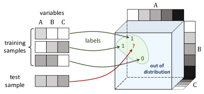
Figure 1: Prediction tasks over discrete variables can be viewed as tensor completion problems. Consider the task of learning a predictor from domain ${\mathcal{X}}=\{1,\ldots,d_{1}\}\times\cdots\times\{1,\ldots,d_{N}\}$ to range ${\mathcal{Y}}={\mathbb{R}}$ (figure assumes $N=3$ and $d_{1}=\cdots=d_{N}=5$ for the sake of illustration). Each input sample is associated with a location in an order $N$ tensor with mode (axis) dimensions $d_{1},\ldots,d_{N}$, where the value of a variable (depicted as a shade of gray) determines the index of the corresponding mode (marked by “A”, “B” or “C”). The associated location stores the label of the sample. Under this viewpoint, training samples are observed entries, drawn according to an unknown distribution from a ground truth tensor. Learning a predictor amounts to completing the unobserved entries, with test error measured by (weighted) average reconstruction error. In many standard prediction tasks (e.g. image recognition), only a small subset of the input domain has non-negligible probability. From the tensor completion perspective this means that observed entries reside in a restricted part of the tensor, and reconstruction error is weighted accordingly (entries outside the support of the distribution are neglected).

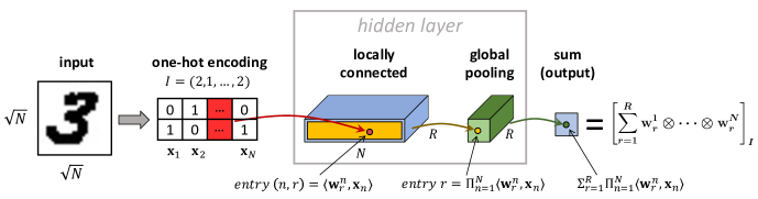
Figure 2: Tensor factorizations correspond to a class of non-linear neural networks. Figure 1 illustrates how a prediction task can be viewed as a tensor completion problem. The current figure extends this correspondence, depicting an equivalence between solving tensor completion via tensor factorization, and learning a predictor using the non-linear neural network portrayed above. The input to the network is a tuple $I=(i_{1},\ldots,i_{N})\in\{1,\ldots,d_{1}\}\times\cdots\times\{1,\ldots,d_{N}\}$, encoded via one-hot vectors $({\mathbf{x}}_{1},\ldots,{\mathbf{x}}_{N})\in{\mathbb{R}}^{d_{1}}\times\cdots\times{\mathbb{R}}^{d_{N}}$. For example, in the diagram, $I$ stands for a binary image with $N$ pixels (in which case $d_{1}=\cdots=d_{N}=2$). The one-hot representations are passed through a hidden layer consisting of: (i) locally connected linear operator with $R$ channels, the $r$’th one computing $\langle{{\mathbf{w}}_{r}^{\scriptscriptstyle 1}},{{\mathbf{x}}_{1}}\rangle,\ldots,\langle{{\mathbf{w}}_{r}^{\scriptscriptstyle N}},{{\mathbf{x}}_{N}}\rangle$ with filters (learnable weights) $\{{\mathbf{w}}_{r}^{\scriptscriptstyle n}\}_{n=1}^{N}$; and (ii) channel-wise global product pooling (multiplicative non-linearity). The resulting activations are then reduced through summation to a scalar — the output of the network. All in all, given input tuple $I=(i_{1},\ldots,i_{N})$, the network outputs the $I$’th entry of $\sum_{r=1}^{R}{\mathbf{w}}_{r}^{\scriptscriptstyle 1}\otimes\cdots\otimes{\mathbf{w}}_{r}^{\scriptscriptstyle N}$. Notice that the number of components $R$ and the weight vectors $\{{\mathbf{w}}_{r}^{\scriptscriptstyle n}\}_{r,n}$ in the factorization correspond to the width and the learnable filters of the network, respectively.

Tensor completion can be viewed as a prediction problem, where each mode corresponds to a discrete input variable. For an unknown tensor ${\mathcal{W}}^{*}\in{\mathbb{R}}^{d_{1},\ldots,d_{N}}$, inputs are index tuples of the form $(i_{1},\ldots,i_{N})$, and the label associated with such an input is $[{\mathcal{W}}^{*}]_{i_{1},\ldots,i_{N}}$. Under this perspective, the training set consists of the observed entries, and the average reconstruction error over unseen entries measures test error. The standard case, in which observations are drawn uniformly across the tensor and reconstruction error weighs all entries equally, corresponds to a data distribution that is uniform, but other distributions are also viable.

Consider for example the task of predicting a continuous label for a $100$-by-$100$ binary image. This can be formulated as an order $10000$ tensor completion problem, where all modes are of dimension $2$. Each input image corresponds to a location (entry) in the tensor ${\mathcal{W}}^{*}$, holding its continuous label. As image pixels are (typically) not distributed independently and uniformly, locations in the tensor are not drawn uniformly when observations are generated, and are not weighted equally when reconstruction error is computed. See Figure 1 for further illustration of how a general prediction task (with discrete inputs and scalar output) can be formulated as a tensor completion problem.

Under the above formulation, tensor factorization can be viewed as a two layer neural network with multiplicative non-linearity. Given an input, i.e. a location in the tensor, the network produces an output equal to the value that the factorization holds at the given location. Figure 2 illustrates this equivalence between solving tensor completion with a tensor factorization and solving a prediction problem with a non-linear neural network. A major drawback of matrix factorization as a theoretical surrogate for modern deep learning is that it misses the critical aspect of non-linearity. Tensor factorization goes beyond the realm of linear predictors — a significant step towards practical neural networks.

3 Dynamical Characterization

In this section we derive a dynamical characterization for the norms of individual components in the tensor factorization. The characterization implies that with small learning rate and near-zero initialization, components tend to be learned incrementally, giving rise to a bias towards low tensor rank solutions. This finding is used in Section 4 to prove (under certain conditions) implicit tensor rank minimization, and is demonstrated empirically in Section 5.

Hereafter, unless specified otherwise, when referring to a norm we mean the standard Frobenius (Euclidean) norm, denoted by $\left\|\cdot\right\|$.

The following lemma establishes an invariant of the dynamics, showing that the differences between squared norms of vectors in the same component are constant through time.

Lemma 1.

For all $r\in\{1,\ldots,R\}$ and $n,\bar{n}\in\{1,\ldots,N\}$:

$$\left\|{\mathbf{w}}_{r}^{n}(t)\right\|^{2}-\left\|{\mathbf{w}}_{r}^{\bar{n}}(t)\right\|^{2}=\left\|{\mathbf{w}}_{r}^{n}(0)\right\|^{2}-\left\|{\mathbf{w}}_{r}^{\bar{n}}(0)\right\|^{2},~{}t\geq 0\text{\,.}$$

Proof sketch (for proof see Lemma 9 in Subappendix C.2.2).

The claim readily follows by showing that under gradient flow $\frac{d}{dt}\|{\mathbf{w}}_{r}^{n}(t)\|^{2}=\frac{d}{dt}\|{\mathbf{w}}_{r}^{\bar{n}}(t)\|^{2}$ for all $t\geq 0$. ∎

Lemma 1 naturally leads to the definition below.

Definition 1.

The unbalancedness magnitude of the weight vectors $\{{\mathbf{w}}_{r}^{n}\in{\mathbb{R}}^{d_{n}}\}_{r=1}^{R}{}_{n=1}^{N}$ is defined to be:

$$\max\nolimits_{r\in\{1,\ldots,R\},~{}n,\bar{n}\in\{1,\ldots,N\}}\left\lvert\left\|{\mathbf{w}}_{r}^{n}\right\|^{2}-\left\|{\mathbf{w}}_{r}^{\bar{n}}\right\|^{2}\right\rvert\text{\,.}$$

By Lemma 1, the unbalancedness magnitude is constant during optimization, and thus, is determined at initialization. When weight vectors are initialized near the origin — regime of interest — the unbalancedness magnitude is small, approaching zero as initialization scale decreases.

Theorem 1 below provides a dynamical characterization for norms of individual components in the tensor factorization.

Theorem 1.

Assume unbalancedness magnitude $\epsilon\geq 0$ at initialization, and denote by ${\mathcal{W}}_{e}(t)$ the end tensor (Equation (3)) at time $t\geq 0$ of optimization. Then, for any $r\in\{1,\ldots,R\}$ and time $t\geq 0$ at which $\|\otimes_{n=1}^{N}{\mathbf{w}}_{r}^{n}(t)\|>0$:

• If $\gamma_{r}(t):=\langle{-\nabla\mathcal{L}({\mathcal{W}}_{e}(t))},{\otimes_{n=1}^{N}\widehat{{\mathbf{w}}}_{r}^{n}(t)}\rangle\geq 0$, then:

  $$\begin{split}&\frac{d}{dt}\|\otimes_{n=1}^{N}{\mathbf{w}}_{r}^{n}(t)\|\leq N\gamma_{r}(t)(\|\otimes_{n=1}^{N}{\mathbf{w}}_{r}^{n}(t)\|^{\frac{2}{N}}+\epsilon)^{N-1}\\ &\frac{d}{dt}\|\otimes_{n=1}^{N}{\mathbf{w}}_{r}^{n}(t)\|\geq N\gamma_{r}(t)\cdot\frac{\|\otimes_{n=1}^{N}{\mathbf{w}}_{r}^{n}(t)\|^{2}}{\|\otimes_{n=1}^{N}{\mathbf{w}}_{r}^{n}(t)\|^{\frac{2}{N}}+\epsilon}\text{\,,}\end{split}$$ (5)

• otherwise, if $\gamma_{r}(t)<0$, then:

  $$\begin{split}&\frac{d}{dt}\|\otimes_{n=1}^{N}{\mathbf{w}}_{r}^{n}(t)\|\geq N\gamma_{r}(t)(\|\otimes_{n=1}^{N}{\mathbf{w}}_{r}^{n}(t)\|^{\frac{2}{N}}+\epsilon)^{N-1}\\ &\frac{d}{dt}\left\|\otimes_{n=1}^{N}{\mathbf{w}}_{r}^{n}(t)\right\|\leq N\gamma_{r}(t)\cdot\frac{\left\|\otimes_{n=1}^{N}{\mathbf{w}}_{r}^{n}(t)\right\|^{2}}{\left\|\otimes_{n=1}^{N}{\mathbf{w}}_{r}^{n}(t)\right\|^{\frac{2}{N}}+\epsilon}\text{\,,}\end{split}$$ (6)

where $\widehat{{\mathbf{w}}}_{r}^{n}(t):={\mathbf{w}}_{r}^{n}(t)/\|{\mathbf{w}}_{r}^{n}(t)\|$ for $n=1,\ldots,N$.

Proof sketch (for proof see Subappendix C.3).

Differentia- ting a component’s norm with respect to time, we obtain $\frac{d}{dt}\|\otimes_{n=1}^{N}{\mathbf{w}}_{r}^{n}(t)\|=\gamma_{r}(t)\cdot\sum_{n=1}^{N}\prod_{n^{\prime}\neq n}\|{\mathbf{w}}_{r}^{n^{\prime}}(t)\|^{2}$. The desired bounds then follow from using conservation of unbalancedness magnitude (as implied by Lemma 1), and showing that $\|{\mathbf{w}}_{r}^{n^{\prime}}(t)\|^{2}\leq\|\otimes_{n=1}^{N}{\mathbf{w}}_{r}^{n}(t)\|^{2/N}+\epsilon$ for all $t\geq 0$ and $n^{\prime}\in\{1,\ldots,N\}$. ∎

Theorem 1 shows that when unbalancedness magnitude at initialization (denoted $\epsilon$) is small, the evolution rates of component norms are roughly proportional to their size exponentiated by $2-2/N$, where $N$ is the order of the tensor factorization. Consequently, component norms are subject to a momentum-like effect, by which they move slower when small and faster when large. This suggests that when initialized near zero, components tend to remain close to the origin, and then, upon reaching a critical threshold, quickly grow until convergence, creating an incremental learning effect that yields implicit regularization towards low tensor rank. This phenomenon is used in Section 4 to formally prove (under certain conditions) implicit tensor rank minimization, and is demonstrated empirically in Section 5.

When the unbalancedness magnitude at initialization is exactly zero, our dynamical characterization takes on a particularly lucid form.

Corollary 1.

Assume unbalancedness magnitude zero at initialization. Then, with notations of Theorem 1, for any $r\in\{1,\ldots,R\}$, the norm of the $r$’th component evolves by:

$$\frac{d}{dt}\left\|\otimes_{n=1}^{N}{\mathbf{w}}_{r}^{n}(t)\right\|=N\gamma_{r}(t)\cdot\left\|\otimes_{n=1}^{N}{\mathbf{w}}_{r}^{n}(t)\right\|^{2-\frac{2}{N}}\text{\,,}$$ (7)

where by convention $\widehat{{\mathbf{w}}}_{r}^{n}(t)=0$ if ${\mathbf{w}}_{r}^{n}(t)=0$.

Proof sketch (for proof see Subappendix C.4).

If the time $t$ is such that $\|\otimes_{n=1}^{N}{\mathbf{w}}_{r}^{n}(t)\|>0$, Equation (7) readily follows from applying Theorem 1 with $\epsilon=0$. For the case where $\|\otimes_{n=1}^{N}{\mathbf{w}}_{r}^{n}(t)\|=0$, we show that the component $\otimes_{n=1}^{N}{\mathbf{w}}_{r}^{n}(t)$ must be identically zero throughout, hence both sides of Equation (7) are equal to zero. ∎

It is worthwhile highlighting the relation to matrix factorization. There, an implicit bias towards low rank emerges from incremental learning dynamics similar to above, with singular values standing in place of component norms. In fact, the dynamical characterization given in Corollary 1 is structurally identical to the one provided by Theorem 3 in Arora et al. (2019) for singular values of a matrix factorization. We thus obtained a generalization from matrices to tensors, notwithstanding the notorious difficulty often associated with the latter (cf. Hillar & Lim (2013)),

4 Implicit Tensor Rank Minimization

In this section we employ the dynamical characterization derived in Section 3 to theoretically establish implicit regularization towards low tensor rank. Specifically, we prove that under certain technical conditions, arbitrarily small initialization leads tensor factorization to follow a trajectory of rank one tensors for an arbitrary amount of time or distance. As a corollary, we obtain that if the tensor completion problem admits a rank one solution, and all rank one trajectories uniformly converge to it, tensor factorization with infinitesimal initialization will converge to it as well. Our analysis generalizes to tensor factorization recent results developed in Li et al. (2021) for matrix factorization. As typical in transitioning from matrices to tensors, this generalization entails significant challenges necessitating use of fundamentally different techniques.

For technical reasons, our focus in this section lies on the Huber loss from robust statistics (Huber, 1964), given by:

$$\ell_{h}:{\mathbb{R}}\,{\to}\,{\mathbb{R}}_{\geq 0}~{},~{}\ell_{h}(z)\,{:=}\begin{cases}\frac{1}{2}z^{2}&,\left\lvert z\right\rvert<\delta_{h}\\ \delta_{h}(\left\lvert z\right\rvert-\frac{1}{2}\delta_{h})&,\text{otherwise}\end{cases}\text{,}$$ (8)

where $\delta_{h}>0$, referred to as the transition point of the loss, is predetermined. Huber loss is often used as a differentiable surrogate for $\ell_{1}$ loss, in which case $\delta_{h}$ is chosen to be small. We will assume it is smaller than observed tensor entries:

Assumption 1.

$\delta_{h}<|y_{i_{1},\ldots,i_{N}}|~{},\forall(i_{1},\ldots,i_{N})\in\Omega$.

We will consider an initialization $\{{\mathbf{a}}_{r}^{n}\in{\mathbb{R}}^{d_{n}}\}_{r=1}^{R}{}_{n=1}^{N}$ for the weight vectors of the tensor factorization, and will scale this initialization towards zero. In line with infinitesimal initializations being captured by unbalancedness magnitude zero (cf. Section 3), we assume that this is the case:

Assumption 2.

The initialization $\{{\mathbf{a}}_{r}^{n}\}_{r=1}^{R}{}_{n=1}^{N}$ has unbalancedness magnitude zero.

We further assume that within $\{{\mathbf{a}}_{r}^{n}\}_{r,n}$ there exists a leading component (subset $\{{\mathbf{a}}_{\bar{r}}^{n}\}_{n}$), in the sense that it is larger than others, while having positive projection on the attracting force at the origin, i.e. on minus the gradient of the loss $\mathcal{L}(\cdot)$ (Equation (1)) at zero:

Assumption 3.

There exists $\bar{r}\in\{1,\ldots,R\}$ such that:

$$\begin{split}&\left\langle{-\nabla\mathcal{L}(0)},{\otimes_{n=1}^{N}\widehat{{\mathbf{a}}}_{\bar{r}}^{n}}\right\rangle>0\text{\,,}\\ &\|{\mathbf{a}}_{\bar{r}}^{n}\|>\|{\mathbf{a}}_{r}^{n}\|{\cdot}\left(\tfrac{\left\|\nabla\mathcal{L}(0)\right\|}{\left\langle{-\nabla\mathcal{L}(0)},{\otimes_{n=1}^{N}\widehat{{\mathbf{a}}}_{\bar{r}}^{n}}\right\rangle}\right)^{1/(N-2)},\forall r\neq\bar{r}\text{\,,}\end{split}$$ (9)

where $\widehat{{\mathbf{a}}}_{\bar{r}}^{n}:={\mathbf{a}}_{\bar{r}}^{n}/\|{\mathbf{a}}_{\bar{r}}^{n}\|$ for $n=1,\ldots,N$.

Let $\alpha>0$, and suppose we run gradient flow on the tensor factorization (see Section 2) starting from the initialization $\{{\mathbf{a}}_{r}^{n}\}_{r,n}$ scaled by $\alpha$. That is, we set:

$${\mathbf{w}}_{r}^{n}(0)=\alpha\cdot{\mathbf{a}}_{r}^{n}\quad,~{}r=1,\ldots,R~{},n=1,\ldots,N\text{\,,}$$

and let $\{{\mathbf{w}}_{r}^{n}(t)\}_{r,n}$ evolve per Equation (4). Denote by ${\mathcal{W}}_{e}(t)$, $t\geq 0$, the trajectory induced on the end tensor (Equation (3)). We will study the evolution of this trajectory through time. A hurdle that immediately arises is that, by the dynamical characterization of Section 3, when the initialization scale $\alpha$ tends to zero (regime of interest), the time it takes ${\mathcal{W}}_{e}(t)$ to escape the origin grows to infinity. We overcome this hurdle by considering a reference sphere — a sphere around the origin with sufficiently small radius:

$${\mathcal{S}}:=\{{\mathcal{W}}\in{\mathbb{R}}^{d_{1},\ldots,d_{N}}:\|{\mathcal{W}}\|=\rho\}\text{\,,}$$ (10)

where $\rho\in(0,\min_{(i_{1},\ldots,i_{N})\in\Omega}\left\lvert y_{i_{1},\ldots,i_{N}}\right\rvert-\delta_{h})$ can be chosen arbitrarily. With the reference sphere ${\mathcal{S}}$ at hand, we define a time-shifted version of the trajectory ${\mathcal{W}}_{e}(t)$, aligning $t=0$ with the moment at which ${\mathcal{S}}$ is reached:

$$\overline{{\mathcal{W}}}_{e}(t):={\mathcal{W}}_{e}\big{(}t+\inf\{t^{\prime}\geq 0:{\mathcal{W}}_{e}(t^{\prime})\in{\mathcal{S}}\}\big{)}\text{\,,}$$ (11)

where by definition $\inf\{t^{\prime}\geq 0:{\mathcal{W}}_{e}(t^{\prime})\in{\mathcal{S}}\}=0$ if ${\mathcal{W}}_{e}(t)$ does not reach ${\mathcal{S}}$. Unlike the original trajectory ${\mathcal{W}}_{e}(t)$, the shifted one $\overline{{\mathcal{W}}}_{e}(t)$ disregards the process of escaping the origin, and thus admits a concrete meaning to the time elapsing from optimization commencement.

We will establish proximity of $\overline{{\mathcal{W}}}_{e}(t)$ to trajectories of rank one tensors. We say that ${\mathcal{W}}_{1}(t)\in{\mathbb{R}}^{d_{1},\ldots,d_{N}}$, $t\geq 0$, is a rank one trajectory, if it coincides with some trajectory of an end tensor in a one-component factorization, i.e. if there exists an initialization for gradient flow over a tensor factorization with $R=1$ components, leading the induced end tensor to evolve by ${\mathcal{W}}_{1}(t)$. If the latter initialization has unbalancedness magnitude zero (cf. Definition 1), we further say that ${\mathcal{W}}_{1}(t)$ is a balanced rank one trajectory.

We are now in a position to state our main result, by which arbitrarily small initialization leads tensor factorization to follow a (balanced) rank one trajectory for an arbitrary amount of time or distance.

Theorem 2.

Under Assumptions 1, 2 and 3, for any distance from origin $D>0$, time duration $T>0$, and degree of approximation $\epsilon\in(0,1)$, if initialization scale $\alpha$ is sufficiently small, then: (i) ${\mathcal{W}}_{e}(t)$ reaches the reference sphere ${\mathcal{S}}$; and (ii) there exists a balanced rank one trajectory ${\mathcal{W}}_{1}(t)$ emanating from ${\mathcal{S}}$, such that $\|\overline{{\mathcal{W}}}_{e}(t)-{\mathcal{W}}_{1}(t)\|\leq\epsilon$ at least until $t\geq T$ or $\|\overline{{\mathcal{W}}}_{e}(t)\|\geq D$.

Proof sketch (for proof see Subappendix C.5).

Using the dynamical characterization from Section 3 (Lemma 1 and Corollary 1), and the fact that $\nabla\mathcal{L}(\cdot)$ is locally constant around the origin, we establish that (i) ${\mathcal{W}}_{e}(t)$ reaches the reference sphere ${\mathcal{S}}$; and (ii) at that time, the norm of the $\bar{r}$’th component is of constant scale (independent of $\alpha$), while the norms of all other components are ${\mathcal{O}}(\alpha^{N})$. Thus, taking $\alpha$ towards zero leads ${\mathcal{W}}_{e}(t)$ to arrive at ${\mathcal{S}}$ while being arbitrarily close to the initialization of a balanced rank one trajectory — ${\mathcal{W}}_{1}(t)$. Since the objective is locally smooth, this ensures $\overline{{\mathcal{W}}}_{e}(t)$ is within distance $\epsilon$ from ${\mathcal{W}}_{1}(t)$ for an arbitrary amount of time or distance. That is, if $\alpha$ is sufficiently small, $\|\overline{{\mathcal{W}}}_{e}(t)-{\mathcal{W}}_{1}(t)\|\leq\epsilon$ at least until $t\geq T$ or $\|\overline{{\mathcal{W}}}_{e}(t)\|\geq D$. ∎

As an immediate corollary of Theorem 2, we obtain that if all balanced rank one trajectories uniformly converge to a global minimum, tensor factorization with infinitesimal initialization will do so too. In particular, its implicit regularization will direct it towards a solution with tensor rank one.

Corollary 2.

Assume the conditions of Theorem 2 (Assumptions 1, 2 and 3), and in addition, that all balanced rank one trajectories emanating from ${\mathcal{S}}$ converge to a tensor ${\mathcal{W}}^{*}\in{\mathbb{R}}^{d_{1},\ldots,d_{N}}$ uniformly, in the sense that they are all confined to some bounded domain, and for any $\epsilon>0$, there exists a time $T$ after which they are all within distance $\epsilon$ from ${\mathcal{W}}^{*}$. Then, for any $\epsilon>0$, if initialization scale $\alpha$ is sufficiently small, there exists a time $T$ for which $\|{\mathcal{W}}_{e}(T)-{\mathcal{W}}^{*}\|\leq\epsilon$.

Proof sketch (for proof see Subappendix C.6).

Let $T^{\prime}>0$ be a time at which all balanced rank one trajectories that emanated from ${\mathcal{S}}$ are within distance $\epsilon/2$ from ${\mathcal{W}}^{*}$. By Theorem 2, if $\alpha$ is sufficiently small, $\overline{{\mathcal{W}}}_{e}(t)$ is guaranteed to be within distance $\epsilon/2$ from a balanced rank one trajectory that emanated from ${\mathcal{S}}$, at least until time $T^{\prime}$. Recalling that $\overline{{\mathcal{W}}}_{e}(t)$ is a time-shifted version of ${\mathcal{W}}_{e}(t)$, the desired result follows from the triangle inequality. ∎

5 Experiments

In this section we present our experiments. Subsection 5.1 corroborates our theoretical analyses (Sections 3 and 4), evaluating tensor factorization (Section 2) on synthetic low (tensor) rank tensor completion problems. Subsection 5.2 explores tensor rank as a measure of complexity, examining its ability to capture the essence of standard datasets. For brevity, we defer a description of implementation details, as well as some experiments, to Appendix B.

5.1 Dynamics of Learning

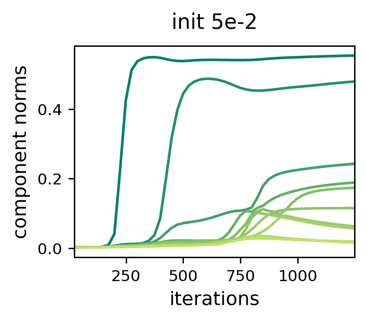
(a)

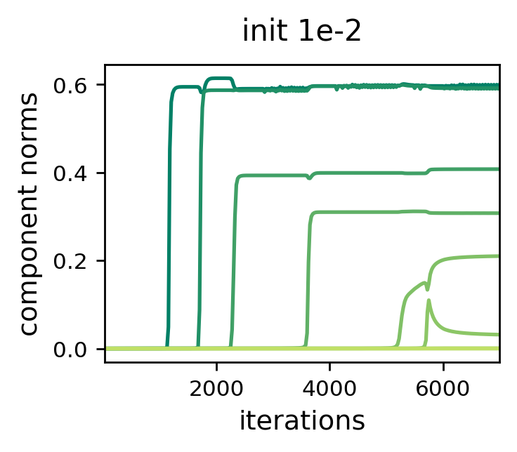
(b)

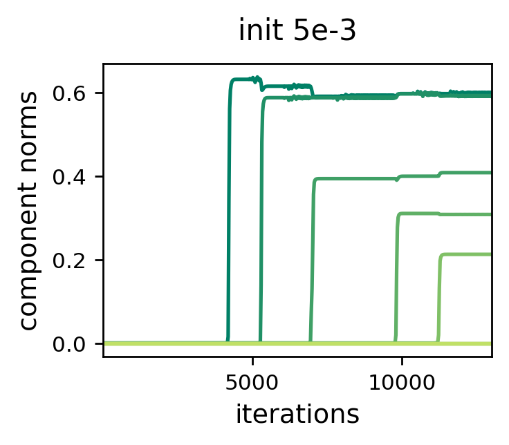
(c)

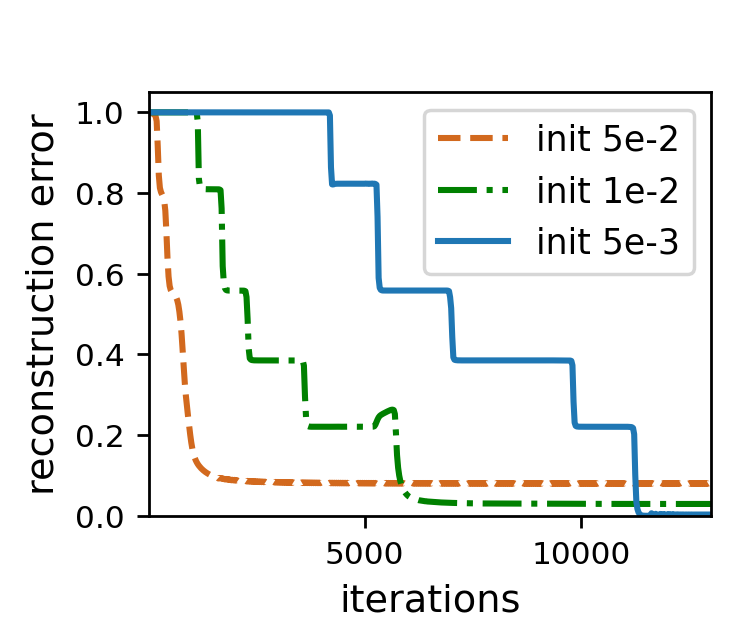
(d)

Figure 3: Dynamics of gradient descent over tensor factorization — incremental learning of components yields low tensor rank solutions. Presented plots correspond to the task of completing a (tensor) rank $5$ ground truth tensor of size $10$-by-$10$-by-$10$-by-$10$ (order $4$) based on $2000$ observed entries chosen uniformly at random without repetition (smaller sample sizes led to solutions with tensor rank lower than that of the ground truth tensor). In each experiment, the $\ell_{2}$ loss (more precisely, Equation (1) with $\ell(z):=z^{2}$) was minimized via gradient descent over a tensor factorization with $R=1000$ components (large enough to express any tensor), starting from (small) random initialization. First (left) three plots show (Frobenius) norms of the ten largest components under three standard deviations for initialization — $0.05,0.01,$ and $0.005$. Further reduction of initialization scale yielded no noticeable change. The rightmost plot compares reconstruction errors (Frobenius distance from ground truth) from the three runs. To facilitate more efficient experimentation, we employed an adaptive learning rate scheme (see Subappendix B.2 for details). Notice that, in accordance with the theoretical analysis of Section 3, component norms move slower when small and faster when large, creating an incremental process in which components are learned one after the other. This effect is enhanced as initialization scale is decreased, producing low tensor rank solutions that accurately reconstruct the low (tensor) rank ground truth tensor. In particular, even though the factorization consists of $1000$ components, when initialization is sufficiently small, only five (tensor rank of the ground truth tensor) substantially depart from zero. Appendix B provides further implementation details, as well as similar experiments with: (i) Huber loss (see Equation (8)) instead of $\ell_{2}$ loss; (ii) ground truth tensors of different orders and (tensor) ranks; and (iii) tensor sensing (see Appendix A).

Recently, Razin & Cohen (2020) empirically showed that, with small learning rate and near-zero initialization, gradient descent over tensor factorization exhibits an implicit regularization towards low tensor rank. Our theory (Sections 3 and 4) explains this implicit regularization through a dynamical analysis — we prove that the movement of component norms is attenuated when small and enhanced when large, thus creating an incremental learning effect which becomes more potent as initialization scale decreases. Figure 3 demonstrates this phenomenon empirically on synthetic low (tensor) rank tensor completion problems. Figures 5, 6 and 7 in Subappendix B.1 extend the experiment, corroborating our analyses in a wide array of settings.

5.2 Tensor Rank as Measure of Complexity

Implicit regularization in deep learning is typically viewed as a tendency of gradient-based optimization to fit training examples with predictors whose “complexity” is as low as possible. The fact that “natural” data gives rise to generalization while other types of data (e.g. random) do not, is understood to result from the former being amenable to fitting by predictors of lower complexity. A major challenge in formalizing this intuition is that we lack definitions for predictor complexity that are both quantitative (i.e. admit quantitative generalization bounds) and capture the essence of natural data (types of data on which neural networks generalize in practice), in the sense of it being fittable with low complexity.

As discussed in Subsection 2.1, learning a predictor with multiple discrete input variables and a continuous output can be viewed as a tensor completion problem. Specifically, with $N\in{\mathbb{N}}$, $d_{1},\ldots,d_{N}\in{\mathbb{N}}$, learning a predictor from domain ${\mathcal{X}}=\{1,\ldots,d_{1}\}\times\cdots\times\{1,\ldots,d_{N}\}$ to range ${\mathcal{Y}}={\mathbb{R}}$ corresponds to completion of an order $N$ tensor with mode (axis) dimensions $d_{1},\ldots,d_{N}$. Under this correspondence, any predictor can simply be thought of as a tensor, and vice versa. We have shown that solving tensor completion via tensor factorization amounts to learning a predictor through a certain neural network (Subsection 2.1), whose implicit regularization favors solutions with low tensor rank (Sections 3 and 4). Motivated by these connections, the current subsection empirically explores tensor rank as a measure of complexity for predictors, by evaluating the extent to which it captures natural data, i.e. allows the latter to be fit with low complexity predictors.

As representatives of natural data, we chose the classic MNIST dataset (LeCun, 1998) — perhaps the most common benchmark for demonstrating ideas in deep learning — and its more modern counterpart Fashion-MNIST (Xiao et al., 2017). A hurdle posed by these datasets is that they involve classification into multiple categories, whereas the equivalence to tensors applies to predictors whose output is a scalar. It is possible to extend the equivalence by equating a multi-output predictor with multiple tensors, in which case the predictor is associated with multiple tensor ranks. However, to facilitate a simple presentation, we avoid this extension and simply map each dataset into multiple one-vs-all binary classification problems. For each problem, we associate the label $1$ with the active category and $0$ with all the rest, and then attempt to fit training examples with predictors of low tensor rank, reporting the resulting mean squared error, i.e. the residual of the fit. This is compared against residuals obtained when fitting two types of random data: one generated via shuffling labels, and the other by replacing inputs with noise.

Figure 4: Evaluation of tensor rank as measure of complexity — standard datasets can be fit accurately with predictors of extremely low tensor rank (far beneath what is required by random datasets), suggesting it may capture the essence of natural data. Left and right plots show results of fitting MNIST and Fashion-MNIST datasets, respectively, with predictors of increasing tensor rank. Original datasets are compared against two random variants: one generated by replacing images with noise (“rand image”), and the other via shuffling labels (“rand label”). As described in the text (Subsection 5.2), for simplicity of presentation, each dataset was mapped into multiple (ten) one-vs-all prediction tasks (label $1$ for active category, $0$ for the rest), with fit measured via mean squared error. Separately for each one-vs-all prediction task and each value $k\in\{1,\ldots,15\}$ for the tensor rank, we applied an approximate numerical method (see Subappendix B.2.2 for details) to find the predictor of tensor rank $k$ (or less) with which the mean squared error over training examples is minimal. We report this mean squared error, as well as that obtained by the predictor on the test set (to mitigate impact of outliers, large squared errors over test samples were clipped — see Subappendix B.2.2 for details). Plots show, for each value of $k$, mean (as marker) and standard deviation (as error bar) of these errors taken over the different one-vs-all prediction tasks. Notice that the original datasets are fit accurately (low train error) by predictors of tensor rank as low as one, whereas random datasets are not (with tensor rank one, residuals of their fit are close to trivial, i.e. to the variance of the label). This suggests that tensor rank as a measure of complexity for predictors has potential to capture the essence of natural data. Notice also that, as expected, accurate fit with low tensor rank coincides with accurate prediction on test set, i.e. with generalization. For further details, as well as an experiment showing that linear predictors are incapable of accurately fitting the datasets, see Appendix B.

Both MNIST and Fashion-MNIST comprise $28$-by-$28$ grayscale images, with each pixel taking one of $256$ possible values. Tensors associated with predictors are thus of order $784$, with dimension $256$ in each mode (axis). A general rank one tensor can then be expressed as an outer product between $784$ vectors of dimension $256$ each, and accordingly has roughly $784\cdot 256$ degrees of freedom. This significantly exceeds the number of training examples in the datasets ($60000$), hence it is no surprise that we could easily fit them, as well as their random variants, with a predictor whose tensor rank is one. To account for the comparatively small training sets, and render their fit more challenging, we quantized pixels to hold one of two values, i.e. we reduced images from grayscale to black and white. Following the quantization, tensors associated with predictors have dimension two in each mode, and the number of degrees of freedom in a general rank one tensor is roughly $784\cdot 2$ — well below the number of training examples. We may thus expect to see a difference between the tensor ranks needed for fitting original datasets and those required by the random ones. This is confirmed by Figure 4, displaying the results of the experiment.

Figure 4 shows that with predictors of low tensor rank, MNIST and Fashion-MNIST can be fit much more accurately than the random datasets. Moreover, as one would presume, accurate fit with low tensor rank coincides with accurate prediction on unseen data (test set), i.e. with generalization. Combined with the rest of our results, we interpret this finding as an indication that tensor rank may shed light on both implicit regularization of neural networks, and the properties of real-world data translating this implicit regularization to generalization.

6 Related Work

Theoretical analysis of implicit regularization induced by gradient-based optimization in deep learning is a highly active area of research. Works along this line typically focus on simplified settings, delivering results such as: characterizations of dynamical or statistical aspects of learning (Du et al., 2018; Gidel et al., 2019; Arora et al., 2019; Brutzkus & Globerson, 2020; Gissin et al., 2020; Chou et al., 2020); solutions for test error when data distribution is known (Advani & Saxe, 2017; Goldt et al., 2019; Lampinen & Ganguli, 2019); and proofs of complexity measures being implicitly minimized in certain situations, either exactly or approximately. The latter type of results is perhaps the most common, covering complexity measures based on: frequency content of input-output mapping (Rahaman et al., 2019; Xu, 2018); curvature of training objective (Mulayoff & Michaeli, 2020); and norm or margin of weights or input-output mapping (Soudry et al., 2018; Gunasekar et al., 2018a, b; Jacot et al., 2018; Ji & Telgarsky, 2019b; Mei et al., 2019; Wu et al., 2020; Nacson et al., 2019; Ji & Telgarsky, 2019a; Oymak & Soltanolkotabi, 2019; Ali et al., 2020; Woodworth et al., 2020; Chizat & Bach, 2020; Yun et al., 2021). An additional complexity measure, arguably the most extensively studied, is matrix rank.

Rank minimization in matrix completion (or sensing) is a classic problem in science and engineering (cf. Davenport & Romberg (2016)). It relates to deep learning when solved via linear neural network, i.e. through matrix factorization. The literature on matrix factorization for rank minimization is far too broad to cover here — we refer to Chi et al. (2019) for a recent review. Notable works proving rank minimization via matrix factorization trained by gradient descent with no explicit regularization are Tu et al. (2016); Ma et al. (2018); Li et al. (2018). Gunasekar et al. (2017) conjectured that this implicit regularization is equivalent to norm minimization, but the recent studies Arora et al. (2019); Razin & Cohen (2020); Li et al. (2021) argue otherwise, and instead adopt a dynamical view, ultimately establishing that (under certain conditions) the implicit regularization in matrix factorization is performing a greedy low rank search. These studies are relevant to ours in the sense that we generalize some of their results to tensor factorization. As typical in transitioning from matrices to tensors (see Hillar & Lim (2013)), this generalization entails significant challenges necessitating use of fundamentally different techniques.

Recovery of low (tensor) rank tensors from incomplete observations via tensor factorizations is a setting of growing interest (cf. Acar et al. (2011); Narita et al. (2012); Anandkumar et al. (2014); Jain & Oh (2014); Yokota et al. (2016); Karlsson et al. (2016); Xia & Yuan (2017); Zhou et al. (2017); Cai et al. (2019) and the survey Song et al. (2019)). However, the experiments of Razin & Cohen (2020) comprise the only evidence we are aware of for successful recovery under gradient-based optimization with no explicit regularization (in particular without imposing low tensor rank through a factorization). The current paper provides the first theoretical support for this implicit regularization.

We note that the equivalence between tensor factorizations and different types of neural networks has been studied extensively, primarily in the context of expressive power (see, e.g., Cohen et al. (2016b); Cohen & Shashua (2016); Sharir et al. (2016); Cohen & Shashua (2017); Cohen et al. (2017); Sharir & Shashua (2018); Levine et al. (2018b); Cohen et al. (2018); Levine et al. (2018a); Balda et al. (2018); Khrulkov et al. (2018); Levine et al. (2019); Khrulkov et al. (2019); Levine et al. (2020)). Connections between tensor analysis and generalization in deep learning have also been made (cf. Li et al. (2020)), but to the best of our knowledge, the notion of quantifying the complexity of predictors through their tensor rank (supported empirically in Subsection 5.2) is novel to this work.

7 Conclusion

In this paper we provided the first theoretical analysis of implicit regularization in tensor factorization. To circumvent the notorious difficulty of tensor problems (see Hillar & Lim (2013)), we adopted a dynamical systems perspective, and characterized the evolution that gradient descent (with small learning rate and near-zero initialization) induces on the components of a factorization. The characterization suggests a form of greedy low tensor rank search, rigorously proven under certain conditions. Experiments demonstrated said phenomena.

A major challenge in mathematically explaining generalization in deep learning is to define measures for predictor complexity that are both quantitative (i.e. admit quantitative generalization bounds) and capture the essence of “natural” data (types of data on which neural networks generalize in practice), in the sense of it being fittable with low complexity. Motivated by the fact that tensor factorization is equivalent to a certain non-linear neural network, and by our analysis implying that the implicit regularization of this network minimizes tensor rank, we empirically explored the potential of the latter to serve as a measure of predictor complexity. We found that it is possible to fit standard image recognition datasets (MNIST and Fashion-MNIST) with predictors of extremely low tensor rank (far beneath what is required for fitting random data), suggesting that it indeed captures aspects of natural data.

The neural network to which tensor factorization is equivalent entails multiplicative non-linearity. It was shown in Cohen & Shashua (2016) that more prevalent non-linearities, for example rectified linear unit (ReLU), can be accounted for by considering generalized tensor factorizations. Studying the implicit regularization in generalized tensor factorizations (both empirically and theoretically) is regarded as a promising direction for future work.

There are two drawbacks to tensor factorization when applied to high-dimensional prediction problems. The first is technical, and relates to numerical stability — an order $N$ tensor factorization involves products of $N$ numbers, thus is susceptible to arithmetic underflow or overflow if $N$ is large. Care should be taken to avoid this pitfall, for example by performing computations in log domain (as done in Cohen & Shashua (2014); Cohen et al. (2016a); Sharir et al. (2016)). The second limitation is more fundamental, arising from the fact that tensor rank — the complexity measure implicitly minimized — is oblivious to the ordering of tensor modes (axes). This means that the implicit regularization does not take into account how predictor inputs are arranged (e.g., in the context of image recognition, it does not take into account spatial relationships between pixels). A potentially promising path for overcoming this limitation is introduction of hierarchy into the tensor factorization, equivalent to adding depth to the corresponding neural network (cf. Cohen et al. (2016b)). It may then be the case that a hierarchical tensor rank (see Hackbusch (2012)), which does account for mode ordering, will be implicitly minimized. We hypothesize that hierarchical tensor ranks may be key to explaining both implicit regularization of contemporary deep neural networks, and the properties of real-world data translating this implicit regularization to generalization.

References

Appendix A Extension to Tensor Sensing

Our theoretical analyses (Sections 3 and 4) are presented in the context of tensor completion, but readily extend to the more general task of tensor sensing — reconstruction of an unknown tensor from linear measurements (projections). In this appendix we outline the extension. Empirical demonstrations for tensor sensing are given in Subappendix B.1 (Figure 7).

For a ground truth tensor ${\mathcal{W}}^{*}\in{\mathbb{R}}^{d_{1},\ldots,d_{N}}$ and measurement tensors $\{{\mathcal{A}}_{i}\in{\mathbb{R}}^{d_{1},\ldots,d_{N}}\}_{i=1}^{m}$, the goal in tensor sensing is to reconstruct ${\mathcal{W}}^{*}$ based on $\{\langle{{\mathcal{A}}_{i}},{{\mathcal{W}}^{*}}\rangle\in{\mathbb{R}}\}_{i=1}^{m}$, where $\left\langle{\,\cdot\,},{\,\cdot\,}\right\rangle$ represents the standard inner product. Similarly to tensor completion (cf. Equation (1)), a standard loss function for the task is:

$$\mathcal{L}_{s}({\mathcal{W}})=\frac{1}{m}\sum\nolimits_{i=1}^{m}\ell\left(\left\langle{{\mathcal{A}}_{i}},{{\mathcal{W}}}\right\rangle-\left\langle{{\mathcal{A}}_{i}},{{\mathcal{W}}^{*}}\right\rangle\right)\text{\,,}$$

where $\mathcal{L}_{s}:{\mathbb{R}}^{d_{1},\ldots,d_{N}}\to{\mathbb{R}}_{\geq 0}$, and $\ell:{\mathbb{R}}\to{\mathbb{R}}_{\geq 0}$ is differentiable and locally smooth. Note that tensor completion is a special case, in which the measurement tensors hold $1$ at a single entry and $0$ elsewhere.

Beginning with Section 3, its results (in particular Lemma 1, Theorem 1 and Corollary 1) hold (and are proven in Subappendix C) for any differentiable and locally smooth $\mathcal{L}(\cdot)$, thus they apply as is to tensor sensing. Turning to Section 4, the extension of Theorem 2 and Corollary 2 to tensor sensing (with Huber loss) is straightforward. Proofs rely on the specifics of tensor completion only in the preliminary Lemmas 12, 13 and 14 (Subappendix C.5.1), for which analogous lemmas may readily be established. Thus, up to slight changes in constants if $\max_{i=1,\ldots,m}\|{\mathcal{A}}_{i}\|>1$, the results carry over.

A.1 Stronger Results Under Restricted Isometry Property

In the classic setting of matrix sensing (tensor sensing with order $N=2$), a commonly studied condition on the measurement matrices is the restricted isometry property. This condition allows for efficient recovery when the ground truth matrix has low rank, and holds with high probability when the entries of the measurement matrices are drawn independently from a zero-mean sub-Gaussian distribution (cf. Recht et al. (2010)). The notion of restricted isometry property extends from matrix to tensor sensing (i.e. from order $N=2$ to arbitrary $N\in{\mathbb{N}}_{\geq 2}$) — see Rauhut et al. (2017); Ibrahim et al. (2020). When it applies, the tensor sensing analogues of Theorem 2 and Corollary 2 can be strengthened as described below.

In the context of tensor sensing, the restricted isometry property is defined as follows.

Definition 2.

We say that the measurement tensors $\{{\mathcal{A}}_{i}\in{\mathbb{R}}^{d_{1},\ldots,d_{N}}\}_{n=1}^{m}$ satisfy $r$-restricted isometry property ($r$-RIP) with parameter $\delta\in[0,1)$ if:

$$(1-\delta)\left\|{\mathcal{W}}\right\|^{2}\leq\sum\nolimits_{i=1}^{m}\left\langle{{\mathcal{A}}_{i}},{{\mathcal{W}}}\right\rangle^{2}\leq(1+\delta)\left\|{\mathcal{W}}\right\|^{2}\text{\,,}$$

for all ${\mathcal{W}}\in{\mathbb{R}}^{d_{1},\ldots,d_{N}}$ of tensor rank $r$ or less.

By Ibrahim et al. (2020), given $m\in{\mathcal{O}}(\log(N)\cdot\sum_{n=1}^{N}d_{n})$ measurement tensors with entries drawn independently from a zero-mean sub-Gaussian distribution, $1$-RIP holds with high probability. In this case, we may strengthen the tensor sensing analogue of Theorem 2, such that it ensures that arbitrarily small initialization leads tensor factorization to follow a rank one trajectory for an arbitrary amount of time, regardless of the distance traveled. That is, with the notations of Theorem 2, for any time duration $T>0$ and degree of approximation $\epsilon\in(0,1)$, if initialization is sufficiently small, $\overline{W}_{e}(t)$ is within $\epsilon$ distance from a balanced rank one trajectory emanating from ${\mathcal{S}}$ at least until time $t\geq T$. To see it is so, notice that since the loss function during gradient flow is monotonically non-increasing, $\sum_{i=1}^{m}\langle{{\mathcal{A}}_{i}},{{\mathcal{W}}_{1}(t)}\rangle^{2}$ is bounded through time for any rank one trajectory ${\mathcal{W}}_{1}(t)$. In turn, since the measurement tensors satisfy $1$-RIP, all such trajectories emanating from ${\mathcal{S}}$ are confined to a ball of radius $D>0$ about the origin, for some $D>0$. By the tensor sensing analogue of Theorem 2, sufficiently small initialization ensures that there exists ${\mathcal{W}}_{1}(t)$ — a balanced rank one trajectory emanating from ${\mathcal{S}}$ — such that $\overline{{\mathcal{W}}}_{e}(t)$ is within $\epsilon$ distance from it at least until $t\geq T$ or $\|\overline{{\mathcal{W}}}_{e}(t)\|\geq D+1$. However, we know that $\|{\mathcal{W}}_{1}(t)\|\leq D$, and so $\overline{{\mathcal{W}}}_{e}(t)$ cannot reach norm of $D+1$ before time $T$, as that would entail a contradiction — $\|{\mathcal{W}}_{1}(t)\|>D$. As a consequence of the above, in the tensor sensing analogue of Corollary 2, when $1$-RIP is satisfied we need not assume all balanced rank one trajectories emanating from ${\mathcal{S}}$ are jointly bounded.

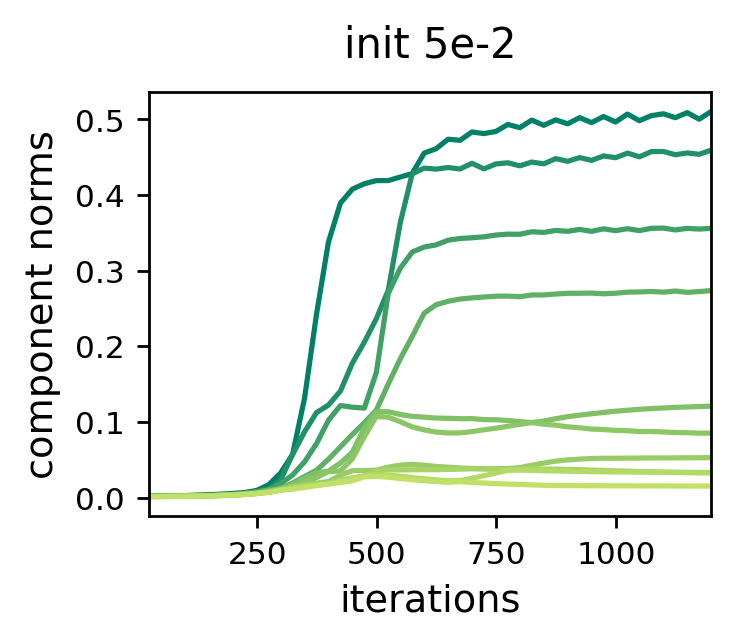
(a)

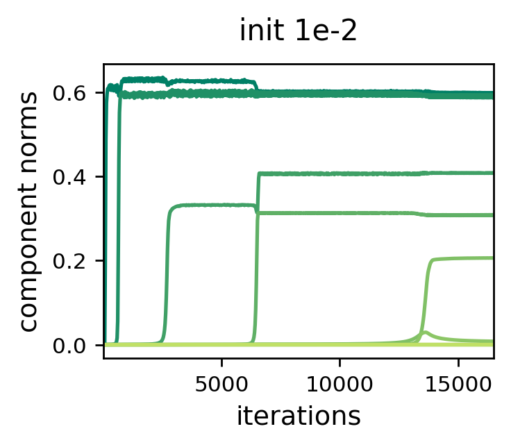
(b)

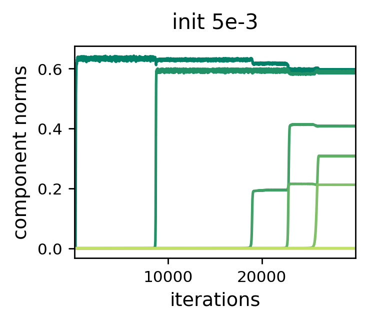
(c)

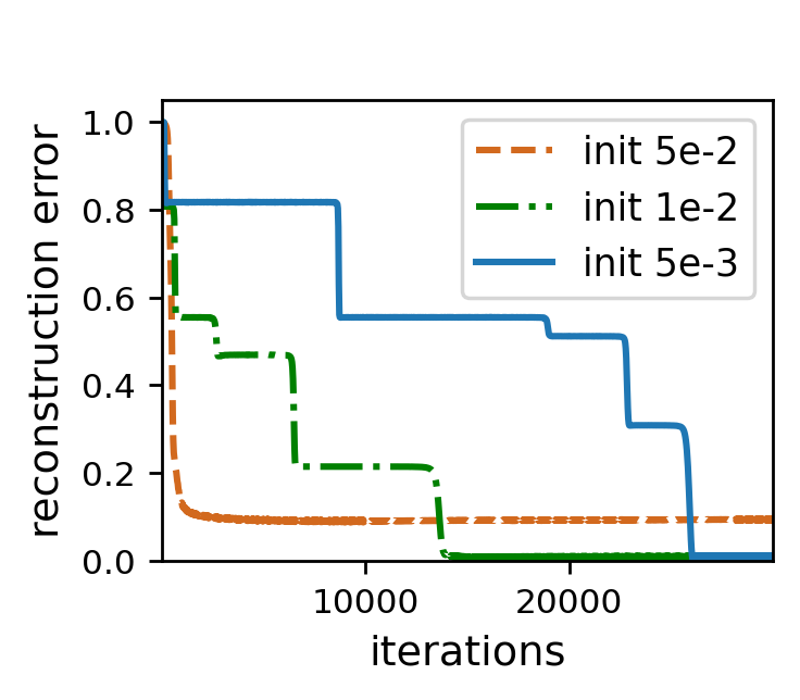
(d)

Figure 5: Dynamics of gradient descent over tensor factorization (with Huber loss) — incremental learning of components yields low tensor rank solutions. This figure is identical to Figure 3, except that the minimized objective (Equation (1)) is based on Huber loss ($\ell_{h}(\cdot)$ from Equation (8)) instead of $\ell_{2}$ loss. In accordance with Assumption 1, the transition point $\delta_{h}$ was set to $5\cdot 10^{-7}$ — smaller than the absolute value of observed entries (though larger $\delta_{h}$ led to similar results). For further details see caption of Figure 3, as well as Subappendix B.2.1.

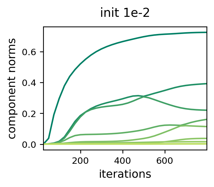
(a)

(b)

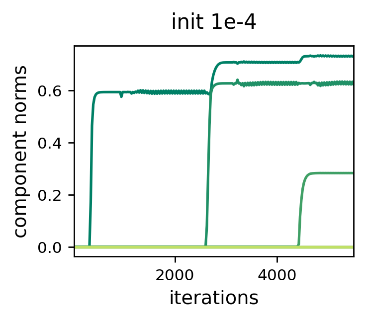
(c)

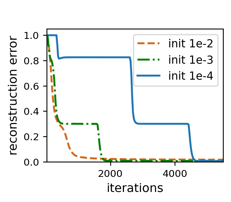
(d)

Figure 6: Dynamics of gradient descent over (order $3$) tensor factorization — incremental learning of components yields low tensor rank solutions. This figure is identical to Figure 3, except that: (i) the ground truth tensor is of (tensor) rank $3$ with size $10$-by-$10$-by-$10$ (order $3$), completed based on $300$ observed entries (smaller sample sizes led to solutions with tensor rank lower than that of the ground truth tensor); and (ii) the employed tensor factorization consists of $R=100$ components (large enough to express any tensor). For further details see caption of Figure 3, as well as Subappendix B.2.1.

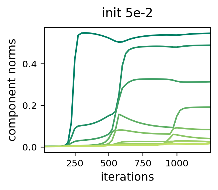
(a)

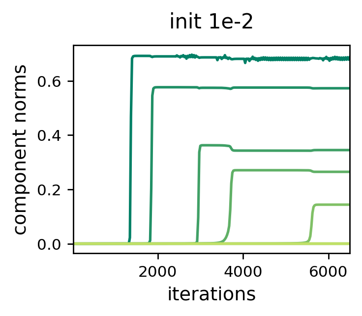
(b)

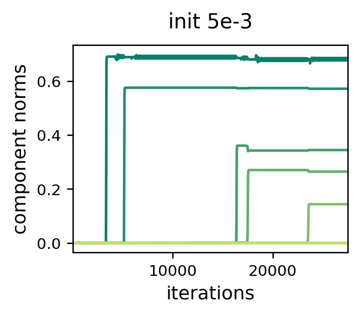
(c)

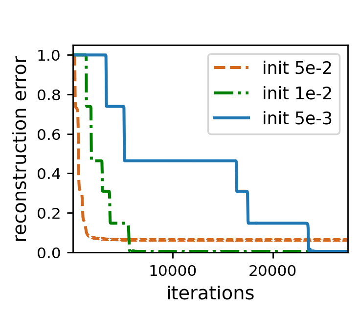
(d)

Figure 7: Dynamics of gradient descent over tensor factorization (on tensor sensing task) — incremental learning of components yields low tensor rank solutions. This figure is identical to Figure 3, except that reconstruction of the ground truth tensor is based on $2000$ linear measurements (instead of $2000$ randomly chosen entries), i.e. on $\{\langle{{\mathcal{A}}_{i}},{{\mathcal{W}}^{*}}\rangle\}_{i=1}^{2000}$, where ${\mathcal{W}}^{*}\in{\mathbb{R}}^{d_{1},\ldots,d_{N}}$ is the ground truth tensor and ${\mathcal{A}}_{1},\ldots,{\mathcal{A}}_{2000}\in{\mathbb{R}}^{d_{1},\ldots,d_{N}}$ are measurement tensors sampled independently from a zero-mean Gaussian distribution (see Appendix A for a description of the tensor sensing task). For further details see caption of Figure 3, as well as Subappendix B.2.1.

Table 1: Linear predictors are incapable of accurately fitting the datasets in the experiment reported by Figure 4. Table presents mean squared errors (over train and test sets) attained by fitting linear predictors to the one-vs-all prediction tasks induced by MNIST and Fashion-MNIST datasets, as well as their random variants (in compliance with Figure 4, to mitigate impact of outliers, large squared errors over test samples were clipped — see Subappendix B.2.2 for details). For each dataset, mean and standard deviation of train and test errors, taken over the different one-vs-all prediction tasks, are reported. Notice that all errors are not far from $0.09$ — the variance of the label — which is trivial to achieve. For further details see caption of Figure 4, as well as Subappendix B.2.2.

	MNIST		Fashion-MNIST
	Train	Test	Train	Test
Original	$3.90\cdot{}10^{-2}$ $\pm$ $8.37\cdot{}10^{-3}$	$3.92\cdot{}10^{-2}$ $\pm$ $8.04\cdot{}10^{-2}$	$4.09\cdot{}10^{-2}$ $\pm$ $1.50\cdot{}10^{-2}$	$4.24\cdot{}10^{-2}$ $\pm$ $1.58\cdot{}10^{-2}$
Rand Image	$8.88\cdot{}10^{-2}$ $\pm$ $4.24\cdot{}10^{-3}$	$9.11\cdot{}10^{-2}$ $\pm$ $4.80\cdot{}10^{-3}$	$8.88\cdot{}10^{-2}$ $\pm$ $3.11\cdot{}10^{-5}$	$9.12\cdot{}10^{-2}$ $\pm$ $2.07\cdot{}10^{-4}$
Rand Label	$8.89\cdot{}10^{-2}$ $\pm$ $4.22\cdot{}10^{-3}$	$9.09\cdot{}10^{-2}$ $\pm$ $4.77\cdot{}10^{-3}$	$8.88\cdot{}10^{-2}$ $\pm$ $7.46\cdot{}10^{-5}$	$9.11\cdot{}10^{-2}$ $\pm$ $2.23\cdot{}10^{-4}$

Appendix B Further Experiments and Implementation Details

B.1 Further Experiments

Figures 5, 6 and 7 supplement Figure 3 from Subsection 5.1 by including, respectively: (i) Huber loss (Equation (8)) instead of $\ell_{2}$ loss; (ii) ground truth tensors of different orders and (tensor) ranks; and (iii) tensor sensing (see Appendix A). Table 1 supplements Figure 4, reporting mean squared errors of linear predictors fitted to the different datasets.

B.2 Implementation Details

Below are implementation details omitted from our experimental reports (Section 5 and Subappendix B.1). Source code for reproducing our results and figures can be found at https://github.com/noamrazin/imp_reg_in_tf (based on the PyTorch framework (Paszke et al., 2017)).

B.2.1 Dynamics of Learning (Figures 3, 5,  6 and 7)

The number of components $R$ was set to ensure an unconstrained search space, i.e. to $10^{2}$ and $10^{3}$ for tensor sizes $10$-by-$10$-by-$10$ and $10$-by-$10$-by-$10$-by-$10$ respectively. Gradient descent was initialized randomly by sampling each weight independently from a zero-mean Gaussian distribution, and was run until the loss reached a value lower than $10^{-8}$ or $10^{6}$ iterations elapsed. For each figure, experiments were carried out with standard deviation of initialization varying over $\{0.05,0.01,0.005,0.001,0.0005,0.0001,0.00005\}$. Reported are representative runs illustrating the different types of dynamics encountered. To facilitate more efficient experimentation, we employed an adaptive learning rate scheme, where at each iteration a base learning rate is divided by the square root of an exponential moving average of squared gradient norms. That is, with base learning rate $\eta=10^{-2}$ and weighted average coefficient $\beta=0.99$, at iteration $t$ the learning rate was set to $\eta_{t}=\eta/(\sqrt{\gamma_{t}/(1-\beta^{t})}+10^{-6})$, where $\gamma_{t}=\beta\cdot\gamma_{t-1}+(1-\beta)\cdot\sum_{r=1}^{R}{}_{n=1}^{N}\|\nicefrac{{\partial}}{{\partial{\mathbf{w}}_{r}^{n}}}\phi(\{{\mathbf{w}}^{n}_{r}(t)\}_{r=1}^{R}{}_{n=1}^{N})\|^{2}$ and $\gamma_{0}=0$. Note that only the learning rate (step size) is affected by this scheme, not the direction of movement. When compared to optimization with a fixed (small) learning rate, no significant difference in the dynamics was observed, while run times were significantly shorter.

Generating a ground truth rank $R^{*}$ tensor ${\mathcal{W}}^{*}\in{\mathbb{R}}^{d_{1},\ldots,d_{N}}$ was done by computing ${\mathcal{W}}^{*}=\sum\nolimits_{r=1}^{R^{*}}{\mathbf{w}}^{*1}_{r}\otimes\cdots\otimes{\mathbf{w}}^{*N}_{r}$, with $\{{\mathbf{w}}^{*n}_{r}\in{\mathbb{R}}^{d_{n}}\}_{r=1}^{R^{*}}{}_{n=1}^{N}$ drawn independently from the standard normal distribution. For convenience, the ground truth tensor was normalized to be of unit Frobenius norm. In tensor completion experiments (Figures 3, 5 and 6), the subset of observed entries was chosen uniformly at random. For tensor sensing (Figure 7), we sampled the entries of all measurement tensors independently from a zero-mean Gaussian distribution with standard deviation $10^{-2}$ (ensures measurement tensors have expected square Frobenius norm of $1$).

B.2.2 Tensor Rank as Measure of Complexity (Figure 4 and Table 1)

For both MNIST and Fashion-MNIST datasets, we quantized pixels to hold either $0$ or $1$ by rounding grayscale values to the nearest integer. Random input datasets were created by replacing all pixels in all images with random values ($0$ or $1$) drawn independently from the uniform distribution. Random label datasets were generated by shuffling labels according to a random permutation, separately for train and test sets.

Given a prediction task, fitting the corresponding tensor completion problem with a predictor of tensor rank $k$ (or less) was done by minimizing the mean squared error over a $k$-component tensor factorization. Stochastic gradient descent, using the Adam optimizer (Kingma & Ba, 2014) with learning rate $5\cdot 10^{-4}$, default $\beta_{1},\beta_{2}$ coefficients, and a batch size of $5000$, was run until the loss reached a value lower than $10^{-8}$ or $10^{4}$ iterations elapsed. For numerical stability, factorization weights were initialized near one. Namely, their initial values were sampled independently from a Gaussian distribution with mean one and standard deviation $10^{-3}$. To accelerate convergence, label values ($0$ or $1$) were scaled up by two during optimization (thereby ensuring symmetry about initialization), with predictions of resulting models scaled down by the same factor during evaluation. Results reported in Table 1 were obtained using the ridge regression implementation of scikit-learn (Pedregosa et al., 2011) with $\alpha=0.5$ (setting $\alpha=0$, i.e. using unregularized linear regression, led to numerical issues due to bad conditioning of the data). Lastly, to mitigate impact of outliers, in both Figure 4 and Table 1 squared errors over test samples were clipped at one, i.e. taken to be the minimum between one and the calculated error.

Appendix C Deferred Proofs

C.1 Notations

For $N\in{\mathbb{N}}$, let $[N]:=\{1,\ldots,N\}$. We use $\left\langle{\cdot},{\cdot}\right\rangle$ to denote the standard Euclidean (Frobenius) inner product between two vectors, matrices, or tensors, and $\left\|\cdot\right\|$ to denote the norm induced by it. Furthermore, we denote the outer and Kronecker products by $\otimes$ and $\odot$, respectively. For a tensor ${\mathcal{W}}\in{\mathbb{R}}^{d_{1},\ldots,d_{N}}$ and $n\in[N]$, we let $\llbracket{\mathcal{W}}\rrbracket_{n}$ be the mode-$n$ matricization of ${\mathcal{W}}$, i.e. its arrangement as a matrix where the rows correspond to the $n$’th mode and the columns correspond to all other modes (see Subsection 2.4 in Kolda & Bader (2009)).

C.2 Useful Lemmas

C.2.1 Technical

Following are several technical lemmas, which are used throughout the proofs.

Lemma 2.

For any ${\mathcal{W}}\in{\mathbb{R}}^{d_{1},\ldots,d_{N}}$ and $\{{\mathbf{w}}^{n}\in{\mathbb{R}}^{d_{n}}\}_{n=1}^{N}$, where $d_{1},\ldots,d_{N}\in{\mathbb{N}}$, it holds that:

$$\left\langle{{\mathcal{W}}},{\otimes_{n^{\prime}=1}^{N}{\mathbf{w}}^{n^{\prime}}}\right\rangle=\left\langle{\llbracket{\mathcal{W}}\rrbracket_{n}\cdot\odot_{n^{\prime}\neq n}{\mathbf{w}}^{n^{\prime}}},{{\mathbf{w}}^{n}}\right\rangle\quad,~{}n=1,\ldots,N\text{\,.}$$

Proof.

To simplify presentation, we prove the equality for $n=1$. For $n=2,\ldots,N$, an analogous computation yields the desired result. By opening up the inner product and applying straightforward computations, we conclude:

$$\begin{split}\left\langle{{\mathcal{W}}},{\otimes_{n^{\prime}=1}^{N}{\mathbf{w}}^{n^{\prime}}}\right\rangle&=\sum_{i_{1}=1}^{d_{1}}\ldots\sum_{i_{N}=1}^{d_{N}}[{\mathcal{W}}]_{i_{1},\ldots,i_{N}}\cdot\prod_{n^{\prime}=1}^{N}[{\mathbf{w}}^{n^{\prime}}]_{i_{n^{\prime}}}\\ &=\sum_{i_{1}=1}^{d_{1}}[{\mathbf{w}}^{1}]_{i_{1}}\sum_{i_{2}=1}^{d_{2}}\ldots\sum_{i_{N}=1}^{d_{N}}[{\mathcal{W}}]_{i_{1},\ldots,i_{N}}\cdot\prod_{n^{\prime}=2}^{N}[{\mathbf{w}}^{n^{\prime}}]_{i_{n^{\prime}}}\\ &=\left\langle{\llbracket{\mathcal{W}}\rrbracket_{1}\cdot\odot_{n^{\prime}=2}^{N}{\mathbf{w}}^{n^{\prime}}},{{\mathbf{w}}^{1}}\right\rangle\text{\,.}\end{split}$$

∎

Lemma 3.

For any $\{{\mathbf{a}}^{n}\in{\mathbb{R}}^{d_{n}}\}_{n=1}^{N},\{{\mathbf{b}}^{n}\in{\mathbb{R}}^{d_{n}}\}_{n=1}^{N}$, where $d_{1},\ldots,d_{N}\in{\mathbb{N}}$, it holds that:

$$\left\|\otimes_{n=1}^{N}{\mathbf{a}}^{n}-\otimes_{n=1}^{N}{\mathbf{b}}^{n}\right\|\leq\sum_{n=1}^{N}\left\|{\mathbf{a}}^{n}-{\mathbf{b}}^{n}\right\|\cdot\prod_{n^{\prime}\neq n}\max\left\{\|{\mathbf{a}}^{n^{\prime}}\|,\|{\mathbf{b}}^{n^{\prime}}\|\right\}\text{\,.}$$

Proof.

The proof is by induction over $N\in{\mathbb{N}}$. For $N=1$, the claim is trivial. Assuming it holds for $N-1\geq 1$, we show that it holds for $N$ as well:

$$\begin{split}\left\|\otimes_{n=1}^{N}{\mathbf{a}}^{n}-\otimes_{n=1}^{N}{\mathbf{b}}^{n}\right\|&=\left\|\otimes_{n=1}^{N}{\mathbf{a}}^{n}-\left(\otimes_{n=1}^{N-1}{\mathbf{a}}^{n}\right)\otimes{\mathbf{b}}^{N}+\left(\otimes_{n=1}^{N-1}{\mathbf{a}}^{n}\right)\otimes{\mathbf{b}}^{N}-\otimes_{n=1}^{N}{\mathbf{b}}^{n}\right\|\\ &\leq\left\|{\mathbf{a}}^{N}-{\mathbf{b}}^{N}\right\|\cdot\left\|\otimes_{n=1}^{N-1}{\mathbf{a}}^{n}\right\|+\left\|\otimes_{n=1}^{N-1}{\mathbf{a}}^{n}-\otimes_{n=1}^{N-1}{\mathbf{b}}^{n}\right\|\cdot\left\|{\mathbf{b}}^{N}\right\|\\ &\leq\left\|{\mathbf{a}}^{N}-{\mathbf{b}}^{N}\right\|\cdot\prod_{n=1}^{N-1}\max\left\{\left\|{\mathbf{a}}^{n}\right\|,\left\|{\mathbf{b}}^{n}\right\|\right\}\\ &\hskip 14.22636pt+\left\|\otimes_{n=1}^{N-1}{\mathbf{a}}^{n}-\otimes_{n=1}^{N-1}{\mathbf{b}}^{n}\right\|\cdot\max\left\{\left\|{\mathbf{a}}^{N}\right\|,\left\|{\mathbf{b}}^{N}\right\|\right\}\text{\,.}\end{split}$$

The proof concludes by the inductive assumption for $N-1$. ∎

Lemma 4.

Let $B_{\left\|\cdot\right\|},B_{dist}>0$ and $\{{\mathbf{a}}_{r}^{n}\in{\mathbb{R}}^{d_{n}}\}_{r=1}^{R}{}_{n=1}^{N},\{{\mathbf{b}}_{r}^{n}\in{\mathbb{R}}^{d_{n}}\}_{r=1}^{R}{}_{n=1}^{N}$, where $d_{1},\ldots,d_{N}\in{\mathbb{N}}$, such that $\max\{\|{\mathbf{a}}_{r}^{n}\|,\|{\mathbf{b}}_{r}^{n}\|\}_{r=1}^{R}{}_{n=1}^{N}\leq B_{\left\|\cdot\right\|}$ and $(\sum_{r=1}^{R}\sum_{n=1}^{N}\|{\mathbf{a}}_{r}^{n}-{\mathbf{b}}_{r}^{n}\|^{2})^{1/2}\leq B_{dist}$. Then:

$$\left\|\sum_{r=1}^{R}\otimes_{n=1}^{N}{\mathbf{a}}_{r}^{n}-\sum_{r=1}^{R}\otimes_{n=1}^{N}{\mathbf{b}}_{r}^{n}\right\|\leq\sqrt{RN}B_{\left\|\cdot\right\|}^{N-1}B_{dist}\text{\,.}$$

Proof.

Applying the triangle inequality and Lemma 3, we have that:

$$\begin{split}\left\|\sum_{r=1}^{R}\otimes_{n=1}^{N}{\mathbf{a}}_{r}^{n}-\sum_{r=1}^{R}\otimes_{n=1}^{N}{\mathbf{b}}_{r}^{n}\right\|&\leq\sum_{r=1}^{R}\left\|\otimes_{n=1}^{N}{\mathbf{a}}_{r}^{n}-\otimes_{n=1}^{N}{\mathbf{b}}_{r}^{n}\right\|\\ &\leq\sum_{r=1}^{R}\sum_{n=1}^{N}\left\|{\mathbf{a}}_{r}^{n}-{\mathbf{b}}_{r}^{n}\right\|\cdot\prod_{n^{\prime}\neq n}\max\left\{\|{\mathbf{a}}_{r}^{n^{\prime}}\|,\|{\mathbf{b}}_{r}^{n^{\prime}}\|\right\}\\ &\leq B_{\left\|\cdot\right\|}^{N-1}\sum_{r=1}^{R}\sum_{n=1}^{N}\left\|{\mathbf{a}}_{r}^{n}-{\mathbf{b}}_{r}^{n}\right\|\text{\,.}\end{split}$$

The desired result readily follows from the fact that $\|{\mathbf{x}}\|_{1}\leq\sqrt{d}\cdot\|{\mathbf{x}}\|$ for any ${\mathbf{x}}\in{\mathbb{R}}^{d}$:

$$\begin{split}\left\|\sum_{r=1}^{R}\otimes_{n=1}^{N}{\mathbf{a}}_{r}^{n}-\sum_{r=1}^{R}\otimes_{n=1}^{N}{\mathbf{b}}_{r}^{n}\right\|&\leq B_{\left\|\cdot\right\|}^{N-1}\sum_{r=1}^{R}\sum_{n=1}^{N}\left\|{\mathbf{a}}_{r}^{n}-{\mathbf{b}}_{r}^{n}\right\|\\ &\leq B_{\left\|\cdot\right\|}^{N-1}\sqrt{RN}\left(\sum_{r=1}^{R}\sum_{n=1}^{N}\left\|{\mathbf{a}}_{r}^{n}-{\mathbf{b}}_{r}^{n}\right\|^{2}\right)^{1/2}\\ &\leq\sqrt{RN}B_{\left\|\cdot\right\|}^{N-1}B_{dist}\text{\,.}\end{split}$$

∎

Lemma 5.

Let $f:[0,T_{2})\to{\mathbb{R}}$ and $g:[0,T_{1})\to{\mathbb{R}}$ be continuous functions, where $T_{1}<T_{2}$. Suppose that $g(t)$ is bounded, $f(0)>0$, and:

$$\frac{d}{dt}f(t)=f(t)^{p}\cdot g(t)\quad,~{}t\in[0,T_{1})\text{\,,}$$ (12)

for $1<p\in{\mathbb{R}}$. Then, $f(t)>0$ for all $t\in[0,T_{1}]$.

Proof.

Consider the initial value problem induced by Equation (12) over the interval $[0,T_{1})$, with an initial value of $f(0)$. One can verify by differentiation that it is solved by:

$$h(t)=\left(f(0)^{1-p}-(p-1)\int_{t^{\prime}=0}^{t}g(t^{\prime})dt^{\prime}\right)^{-\frac{1}{p-1}}\text{\,.}$$

Since the problem has a unique solution (see, e.g., Theorem 2.2 in Teschl (2012)), it follows that for any $t\in[0,T_{1})$:

$$f(t)=h(t)=\left(f(0)^{1-p}-(p-1)\int_{t^{\prime}=0}^{t}g(t^{\prime})dt^{\prime}\right)^{-\frac{1}{p-1}}\geq\left(f(0)^{1-p}+(p-1)\int_{t^{\prime}=0}^{t}\left\lvert g(t^{\prime})\right\rvert dt^{\prime}\right)^{-\frac{1}{p-1}}\text{\,.}$$

Recall that $g(t)$ is bounded. Hence, from the inequality above and continuity of $f(\cdot)$ we conclude:

$$f(t)\geq\left(f(0)^{1-p}+(p-1)\cdot\sup\nolimits_{t^{\prime}\in[0,T_{1})}\left\lvert g(t^{\prime})\right\rvert\cdot T_{1}\right)^{-\frac{1}{p-1}}>0~{}~{},~{}t\in[0,T_{1}]\text{\,.}$$

∎

Lemma 6.

Let $\theta,\theta^{\prime}:[0,T]\to{\mathbb{R}}^{d}$, where $T>0$, be two curves born from gradient flow over a continuously differentiable function $f:{\mathbb{R}}^{d}\to{\mathbb{R}}$:

$$\theta(0)=\theta_{0}\in{\mathbb{R}}^{d}~{} ~{}\tfrac{d}{dt}\theta(t)=-\nabla f(\theta(t))~{}~{},~{}t\in[0,T]\text{\,,}$$ ,

$$\theta^{\prime}(0)=\theta^{\prime}_{0}\in{\mathbb{R}}^{d}~{} ~{}\tfrac{d}{dt}\theta^{\prime}(t)=-\nabla f(\theta^{\prime}(t))~{}~{},~{}t\in[0,T]\text{\,.}$$ ,

Let $D>0$, and suppose that $f(\cdot)$ is $\beta$-smooth over ${\mathcal{D}}_{D+1}$ for some $\beta\geq 0$, where ${\mathcal{D}}_{D+1}:=\{\theta\in{\mathbb{R}}^{d}:\|\theta\|\leq D+1\}$. Then, if $\|\theta(0)-\theta^{\prime}(0)\|<\exp(-\beta\cdot T)$, it holds that:

$$\left\|\theta(t)-\theta^{\prime}(t)\right\|\leq\left\|\theta(0)-\theta^{\prime}(0)\right\|\cdot\exp\left(\beta\cdot t\right)\text{\,}$$ (13)

at least until $t\geq T$ or $\|\theta^{\prime}(t)\|\geq D$. That is, Equation (13) holds for all $t\in[0,\min\{T,T_{D}\}]$, where $T_{D}:=\inf\{t\geq 0:\|\theta^{\prime}(t)\|\geq D\}$.

Proof.

If $\|\theta^{\prime}(0)\|\geq D$, the claim trivially holds. Suppose $\|\theta^{\prime}(0)\|<D$, and notice that in this case $\|\theta(0)\|<\|\theta^{\prime}(0)\|+\exp(-\beta\cdot T)<D+1$. We examine the initial time at which $\|\theta^{\prime}(t)\|\geq D$ or $\|\theta(t)\|\geq D+1$. That is, let $\widebar{T}_{D}:=\inf\left\{t\in[0,T]:\|\theta^{\prime}(t)\|\geq D\text{ or }\|\theta(t)\|\geq D+1\right\}$, where we take $\widebar{T}_{D}:=T$ if the set is empty. Since both $\left\|\theta^{\prime}(t)\right\|$ and $\left\|\theta(t)\right\|$ are continuous in $t$, it must be that $\widebar{T}>0$. Furthermore, $\left\|\theta^{\prime}(t)\right\|\leq D$ and $\left\|\theta(t)\right\|\leq D+1$ for all $t\in[0,\widebar{T}_{D}]$.

Now, define the function $g:[0,T]\to{\mathbb{R}}_{\geq 0}$ by $g(t):=\left\|\theta(t)-\theta^{\prime}(t)\right\|^{2}$. For any $t\in[0,\widebar{T}_{D}]$ it holds that:

$$\begin{split}\frac{d}{dt}g(t)&=2\left\langle{\theta(t)-\theta^{\prime}(t)},{\tfrac{d}{dt}\theta(t)-\tfrac{d}{dt}\theta^{\prime}(t)}\right\rangle\\ &=-2\left\langle{\theta(t)-\theta^{\prime}(t)},{\nabla f(\theta(t))-\nabla f(\theta^{\prime}(t))}\right\rangle\text{\,.}\end{split}$$

By the Cauchy-Schwartz inequality and $\beta$-smoothness of $f(\cdot)$ over ${\mathcal{D}}_{D+1}$ we have:

$$\begin{split}\frac{d}{dt}g(t)&\leq 2\beta\cdot\left\|\theta(t)-\theta^{\prime}(t)\right\|^{2}=2\beta\cdot g(t)\text{\,.}\end{split}$$ (14)

Thus, Gronwall’s inequality leads to $g(t)\leq g(0)\cdot\exp(2\beta\cdot t)$. Taking the square root of both sides then establishes Equation (13) for all $t\in[0,\widebar{T}_{D}]$.

If $\widebar{T}_{D}=T$, the proof concludes since Equation (13) holds over $[0,T]$. Otherwise, if $\widebar{T}_{D}<T$, then either $\|\theta^{\prime}(\widebar{T}_{D})\|=D$ or $\|\theta(\widebar{T}_{D})\|=D+1$. It suffices to show that in both cases $T_{D}\leq\widebar{T}_{D}$. In case $\|\theta^{\prime}(\widebar{T}_{D})\|=D$, the definition of $T_{D}$ implies $T_{D}=\widebar{T}_{D}$. On the other hand, suppose $\|\theta(\widebar{T}_{D})\|=D+1$. Since $\left\|\theta(0)-\theta^{\prime}(0)\right\|<\exp(-\beta\cdot T)$, the fact that Equation (13) holds for $\widebar{T}_{D}$ gives $\left\|\theta(\widebar{T}_{D})-\theta^{\prime}(\widebar{T}_{D})\right\|\leq 1$. Therefore, it must be that $\left\|\theta^{\prime}(\widebar{T}_{D})\right\|\geq D$, and so $T_{D}\leq\widebar{T}_{D}$, completing the proof. ∎

C.2.2 Tensor Factorization

Suppose that we minimize the objective $\phi(\cdot)$ (Equations (2) and (3)) via gradient flow over an $R$-component tensor factorization (Equation (4)), where we allow the loss $\mathcal{L}(\cdot)$ in Equation (2) to be any differentiable and locally smooth function. Under this setting, the following lemmas establish several results which will be of use when proving the main theorems.

Lemma 7.

For any $\{{\mathbf{w}}_{r}^{n}\in{\mathbb{R}}^{d_{n}}\}_{r=1}^{R}{}_{n=1}^{N}$:

$$\frac{\partial}{\partial{\mathbf{w}}_{r}^{n}}\phi\left(\{{\mathbf{w}}_{r^{\prime}}^{n^{\prime}}\}_{r^{\prime}=1}^{R}{}_{n^{\prime}=1}^{N}\right)=\llbracket\nabla\mathcal{L}\left({\mathcal{W}}_{e}\right)\rrbracket_{n}\cdot\odot_{n^{\prime}\neq n}{\mathbf{w}}_{r}^{n^{\prime}}\quad,~{}r=1,\ldots,R~{},~{}n=1,\ldots,N\text{\,,}$$

where ${\mathcal{W}}_{e}$ denotes the end tensor (Equation (3)) induced by $\{{\mathbf{w}}_{r}^{n}\}_{r=1}^{R}{}_{n=1}^{N}$.

Proof.

For $r\in[R],n\in[N]$, we treat $\{{\mathbf{w}}_{r^{\prime}}^{n^{\prime}}\}_{(r^{\prime},n^{\prime})\neq(r,n)}$ as fixed, and with slight abuse of notation consider:

$$\phi_{r,n}\left({\mathbf{w}}_{r}^{n}\right):=\phi\left(\{{\mathbf{w}}_{r^{\prime}}^{n^{\prime}}\}_{r^{\prime}=1}^{R}{}_{n^{\prime}=1}^{N}\right)\text{\,.}$$

For $\Delta\in{\mathbb{R}}^{d_{n}}$, from the first order Taylor approximation of $\mathcal{L}(\cdot)$ we have that:

$$\begin{split}\phi_{r,n}\left({\mathbf{w}}_{r}^{n}+\Delta\right)&=\mathcal{L}\left({\mathcal{W}}_{e}+\left(\otimes_{n^{\prime}=1}^{n-1}{\mathbf{w}}_{r}^{n^{\prime}}\right)\otimes\Delta\otimes\left(\otimes_{n^{\prime}=n+1}^{N}{\mathbf{w}}_{r}^{n^{\prime}}\right)\right)\\ &=\mathcal{L}\left({\mathcal{W}}_{e}\right)+\left\langle{\nabla\mathcal{L}\left({\mathcal{W}}_{e}\right)},{\left(\otimes_{n^{\prime}=1}^{n-1}{\mathbf{w}}_{r}^{n^{\prime}}\right)\otimes\Delta\otimes\left(\otimes_{n^{\prime}=n+1}^{N}{\mathbf{w}}_{r}^{n^{\prime}}\right)}\right\rangle+o\left(\left\|\Delta\right\|\right)\text{\,.}\end{split}$$

Since $\mathcal{L}\left({\mathcal{W}}_{e}\right)=\phi_{r,n}({\mathbf{w}}_{r}^{n})$, by applying Lemma 2 we arrive at:

$$\phi_{r,n}\left({\mathbf{w}}_{r}^{n}+\Delta\right)=\phi_{r,n}\left({\mathbf{w}}_{r}^{n}\right)+\left\langle{\llbracket\nabla\mathcal{L}({\mathcal{W}}_{e})\rrbracket_{n}\cdot\odot_{n^{\prime}\neq n}{\mathbf{w}}_{r}^{n^{\prime}}},{\Delta}\right\rangle+o(\left\|\Delta\right\|)\text{\,.}$$

Uniqueness of the linear approximation of $\phi_{r,n}(\cdot)$ at ${\mathbf{w}}_{r}^{n}$ then implies:

$$\frac{\partial}{\partial{\mathbf{w}}_{r}^{n}}\phi\left(\{{\mathbf{w}}_{r^{\prime}}^{n^{\prime}}\}_{r^{\prime}=1}^{R}{}_{n^{\prime}=1}^{N}\right)=\frac{d}{d{\mathbf{w}}_{r}^{n}}\phi_{r,n}\left({\mathbf{w}}_{r}^{n}\right)=\llbracket\nabla\mathcal{L}\left({\mathcal{W}}_{e}\right)\rrbracket_{n}\cdot\odot_{n^{\prime}\neq n}{\mathbf{w}}_{r}^{n^{\prime}}\text{\,.}$$

∎

Lemma 8.

For any $r\in[R]$ and $n\in[N]$:

$$\frac{d}{dt}\|{\mathbf{w}}_{r}^{n}(t)\|^{2}=-2\left\langle{\nabla\mathcal{L}\left({\mathcal{W}}_{e}(t)\right)},{\otimes_{n^{\prime}=1}^{N}{\mathbf{w}}_{r}^{n^{\prime}}(t)}\right\rangle\text{\,.}$$

Proof.

Fix $r\in[R]$ and $n\in[N]$. Differentiating $\|{\mathbf{w}}_{r}^{n}(t)\|^{2}$ with respect to time, we have:

$$\frac{d}{dt}\|{\mathbf{w}}_{r}^{n}(t)\|^{2}=2\left\langle{{\mathbf{w}}_{r}^{n}(t)},{\tfrac{d}{dt}{\mathbf{w}}_{r}^{n}(t)}\right\rangle=-2\left\langle{{\mathbf{w}}_{r}^{n}(t)},{\frac{\partial}{\partial{\mathbf{w}}_{r}^{n}}\phi\left(\{{\mathbf{w}}_{r^{\prime}}^{n^{\prime}}(t)\}_{r^{\prime}=1}^{R}{}_{n^{\prime}=1}^{N}\right)}\right\rangle\text{\,.}$$

Applying Lemmas 7 and 2 completes the proof. ∎

Lemma 9 (Lemma 1 restated).

For all $r\in[R]$ and $n,\bar{n}\in[N]$:

$$\left\|{\mathbf{w}}_{r}^{n}(t)\right\|^{2}-\left\|{\mathbf{w}}_{r}^{\bar{n}}(t)\right\|^{2}=\left\|{\mathbf{w}}_{r}^{n}(0)\right\|^{2}-\left\|{\mathbf{w}}_{r}^{\bar{n}}(0)\right\|^{2}\quad,~{}t\geq 0\text{\,.}$$

Proof of Lemma 9.

For any $r\in[R]$ and $n,\bar{n}\in[N]$, by Lemma 8 it holds that:

$$\frac{d}{dt}\|{\mathbf{w}}_{r}^{n}(t)\|^{2}=-2\left\langle{\nabla\mathcal{L}\left({\mathcal{W}}_{e}(t)\right)},{\otimes_{n^{\prime}=1}^{N}{\mathbf{w}}_{r}^{n^{\prime}}(t)}\right\rangle=\frac{d}{dt}\|{\mathbf{w}}_{r}^{\bar{n}}(t)\|^{2}\text{\,.}$$

Integrating both sides with respect to time gives:

$$\left\|{\mathbf{w}}_{r}^{n}(t)\right\|^{2}-\left\|{\mathbf{w}}_{r}^{n}(0)\right\|^{2}=\left\|{\mathbf{w}}_{r}^{\bar{n}}(t)\right\|^{2}-\left\|{\mathbf{w}}_{r}^{\bar{n}}(0)\right\|^{2}\text{\,.}$$

Rearranging the equality above establishes the desired result. ∎

Lemma 10.

Let $\widetilde{R}>R$, and define:

$$\widetilde{{\mathbf{w}}}_{r}^{n}(t):=\begin{cases}{\mathbf{w}}_{r}^{n}(t)&,r\in\{1,\ldots,R\}\\ 0\in{\mathbb{R}}^{d_{n}}&,r\in\{R+1,\ldots,\widetilde{R}\}\end{cases}\quad,~{}t\geq 0~{},~{}n=1,\ldots,N\text{\,.}$$ (15)

Then, $\{\widetilde{{\mathbf{w}}}_{r}^{n}(t)\}_{r=1}^{\widetilde{R}}{}_{n=1}^{N}$ follow a gradient flow path of an $\widetilde{R}$-component factorization.

Proof.

We verify that $\{\widetilde{{\mathbf{w}}}_{r}^{n}(t)\}_{r=1}^{\widetilde{R}}{}_{n=1}^{N}$ satisfy the differential equations governing gradient flow. Fix $n\in[N]$. For any $r\in[R]$ and $t\geq 0$ we have:

$$\begin{split}\frac{d}{dt}\widetilde{{\mathbf{w}}}_{r}^{n}(t)&=\frac{d}{dt}{\mathbf{w}}_{r}^{n}(t)=-\frac{\partial}{\partial{\mathbf{w}}_{r}^{n}}\phi\left(\{{\mathbf{w}}_{r^{\prime}}^{n^{\prime}}(t)\}_{r^{\prime}=1}^{R}{}_{n^{\prime}=1}^{N}\right)\text{\,.}\end{split}$$

Noticing that ${\mathcal{W}}_{e}(t)=\sum_{r^{\prime}=1}^{R}\otimes_{n^{\prime}=1}^{N}{\mathbf{w}}_{r^{\prime}}^{n^{\prime}}(t)=\sum_{r^{\prime}=1}^{\widetilde{R}}\otimes_{n^{\prime}=1}^{N}\widetilde{{\mathbf{w}}}_{r^{\prime}}^{n^{\prime}}(t)=\widetilde{{\mathcal{W}}}_{e}(t)$, and invoking Lemma 7, we may write:

$$\begin{split}\frac{d}{dt}\widetilde{{\mathbf{w}}}_{r}^{n}(t)&=-\left\llbracket\nabla\mathcal{L}\left({\mathcal{W}}_{e}(t)\right)\right\rrbracket_{n}\cdot\odot_{n^{\prime}\neq n}{\mathbf{w}}_{r}^{n^{\prime}}(t)\\ &=-\left\llbracket\nabla\mathcal{L}\left(\widetilde{{\mathcal{W}}}_{e}(t)\right)\right\rrbracket_{n}\cdot\odot_{n^{\prime}\neq n}\widetilde{{\mathbf{w}}}_{r}^{n^{\prime}}(t)\\ &=-\frac{\partial}{\partial\widetilde{{\mathbf{w}}}_{r}^{n}}\phi\left(\{\widetilde{{\mathbf{w}}}_{r^{\prime}}^{n^{\prime}}(t)\}_{r^{\prime}=1}^{\widetilde{R}}{}_{n^{\prime}=1}^{N}\right)\text{\,.}\end{split}$$

On the other hand, for any $r\in\{R+1,\ldots,\widetilde{R}\}$, recalling that $\widetilde{{\mathbf{w}}}_{r}^{n}(t)$ is identically zero:

$$\begin{split}\frac{d}{dt}\widetilde{{\mathbf{w}}}_{r}^{n}(t)=0=-\left\llbracket\nabla\mathcal{L}\left(\widetilde{{\mathcal{W}}}_{e}(t)\right)\right\rrbracket_{n}\cdot\odot_{n^{\prime}\neq n}\widetilde{{\mathbf{w}}}_{r}^{n^{\prime}}(t)=-\frac{\partial}{\partial\widetilde{{\mathbf{w}}}_{r}^{n}}\phi\left(\{\widetilde{{\mathbf{w}}}_{r^{\prime}}^{n^{\prime}}(t)\}_{r^{\prime}=1}^{\widetilde{R}}{}_{n^{\prime}=1}^{N}\right)\text{\,,}\end{split}$$

for all $t\geq 0$, completing the proof. ∎

Lemma 11.

For any $r\in[R]$:

• If $\|{\mathbf{w}}_{r}^{1}(0)\|=\cdots=\|{\mathbf{w}}_{r}^{N}(0)\|=0$, then:

  $$\left\|{\mathbf{w}}_{r}^{1}(t)\right\|=\cdots=\left\|{\mathbf{w}}_{r}^{N}(t)\right\|=0\quad,~{}t\geq 0\text{\,.}$$ (16)

• On the other hand, if $\|{\mathbf{w}}_{r}^{1}(0)\|=\cdots=\|{\mathbf{w}}_{r}^{N}(0)\|>0$, then:

  $$\left\|{\mathbf{w}}_{r}^{1}(t)\right\|=\cdots=\left\|{\mathbf{w}}_{r}^{N}(t)\right\|>0\quad,~{}t\geq 0\text{\,.}$$ (17)

Proof.

The proof is divided into two separate parts, establishing Equations (16) and (17) under their respective conditions.

Proof of Equation (16) (if $\|{\mathbf{w}}_{r}^{1}(0)\|=\cdots=\|{\mathbf{w}}_{r}^{N}(0)\|=0$):

To simplify presentation, we assume without loss of generality that $r=R$. Consider the following initial value problem induced by gradient flow over $\phi(\cdot)$:

$$\begin{split}&\widetilde{{\mathbf{w}}}_{\bar{r}}^{n}(0)={\mathbf{w}}_{\bar{r}}^{n}(0)\quad,~{}\bar{r}=1,\ldots,R~{},~{}n=1,\ldots,N\text{\,,}\\ &\frac{d}{dt}\widetilde{{\mathbf{w}}}_{\bar{r}}^{n}(t)=-\frac{\partial}{\partial\widetilde{{\mathbf{w}}}_{\bar{r}}^{n}}\phi\left(\{\widetilde{{\mathbf{w}}}_{r^{\prime}}^{n^{\prime}}(t)\}_{r^{\prime}=1}^{R}{}_{n^{\prime}=1}^{N}\right)\quad,~{}t\geq 0~{},~{}\bar{r}=1,\ldots,R~{},~{}n=1,\ldots,N\text{\,.}\end{split}$$ (18)

By definition, $\{{\mathbf{w}}_{\bar{r}}^{n}(t)\}_{\bar{r}=1}^{R}{}_{n=1}^{N}$ is a solution to the initial value problem above. Since it has a unique solution (see, e.g., Theorem 2.2 in Teschl (2012)), we need only show that there exist $\{\widetilde{{\mathbf{w}}}_{\bar{r}}^{n}(t)\}_{\bar{r}=1}^{R}{}_{n=1}^{N}$ satisfying Equation (18) such that $\widetilde{{\mathbf{w}}}_{R}^{1}(t)=\cdots=\widetilde{{\mathbf{w}}}_{R}^{N}(t)=0$ for all $t\geq 0$.

If $R=1$, i.e. the factorization consists of a single component, by Lemma 7:

$$-\frac{\partial}{\partial\widetilde{{\mathbf{w}}}_{1}^{n}}\phi\left(\{\widetilde{{\mathbf{w}}}_{1}^{n^{\prime}}\}_{n^{\prime}=1}^{N}\right)=-\left\llbracket\nabla\mathcal{L}\left(\otimes_{n^{\prime}=1}^{N}\widetilde{{\mathbf{w}}}_{1}^{n^{\prime}}\right)\right\rrbracket_{n}\cdot\odot_{n^{\prime}\neq n}\widetilde{{\mathbf{w}}}_{1}^{n^{\prime}}\quad,~{}n=1,\ldots,N\text{\,,}$$

for any $\widetilde{{\mathbf{w}}}_{1}^{1}\in{\mathbb{R}}^{d_{1}},\ldots,\widetilde{{\mathbf{w}}}_{1}^{N}\in{\mathbb{R}}^{d_{N}}$. Hence, $\widetilde{{\mathbf{w}}}_{1}^{1}(t)=\cdots=\widetilde{{\mathbf{w}}}_{1}^{N}(t)=0$ for all $t\geq 0$ form a solution to the initial value problem in Equation (18). To see it is so, notice that the initial conditions are met, and:

$$\frac{d}{dt}\widetilde{{\mathbf{w}}}_{1}^{n}(t)=0=-\frac{\partial}{\partial\widetilde{{\mathbf{w}}}_{1}^{n}}\phi\left(\{\widetilde{{\mathbf{w}}}_{1}^{n^{\prime}}(t)\}_{n^{\prime}=1}^{N}\right)\quad,~{}t\geq 0~{},~{}n=1,\ldots,N\text{\,.}$$

If $R>1$, with slight abuse of notation we denote by $\phi(\{\widetilde{{\mathbf{w}}}_{\bar{r}}^{n}\}_{\bar{r}=1}^{R-1}{}_{n=1}^{N}):=\mathcal{L}(\sum_{\bar{r}=1}^{R-1}\otimes_{n=1}^{N}\widetilde{{\mathbf{w}}}_{\bar{r}}^{n})$ the objective over an $(R-1)$-component tensor factorization. Let $\{\widetilde{{\mathbf{w}}}_{\bar{r}}^{n}(t)\}_{\bar{r}=1}^{R-1}{}_{n=1}^{N}$ be curves obtained by running gradient flow on this objective, initialized such that:

$$\widetilde{{\mathbf{w}}}_{\bar{r}}^{n}(0):={\mathbf{w}}_{\bar{r}}^{n}(0)\quad,~{}\bar{r}=1,\ldots,R-1~{},~{}n=1,\ldots,N\text{\,.}$$

Additionally, define $\widetilde{{\mathbf{w}}}_{R}^{1}(t)=\cdots=\widetilde{{\mathbf{w}}}_{R}^{N}(t)=0$ for all $t\geq 0$. According to Lemma 10, $\{\widetilde{{\mathbf{w}}}_{\bar{r}}^{n}(t)\}_{\bar{r}=1}^{R}{}_{n=1}^{N}$ form a valid solution to the original gradient flow over an $R$-component factorization, i.e. satisfy Equation (18). Thus, uniqueness of the solution implies ${\mathbf{w}}_{R}^{1}(t)=\cdots={\mathbf{w}}_{R}^{N}(t)=0$ for all $t\geq 0$, completing the proof for Equation (16).

Proof of Equation (17) (if $\|{\mathbf{w}}_{r}^{1}(0)\|=\cdots=\|{\mathbf{w}}_{r}^{N}(0)\|>0$):

From Lemma 1 it follows that $\|{\mathbf{w}}_{r}^{1}(t)\|=\cdots=\|{\mathbf{w}}_{r}^{N}(t)\|$ for any $t\geq 0$. Hence, it suffices to show that $\|{\mathbf{w}}_{r}^{1}(t)\|$ stays positive. Assume by way of contradiction that there exists $\bar{t}>0$ for which $\|{\mathbf{w}}_{r}^{1}(\bar{t}\,)\|=0$. Define:

$$t_{0}:=\inf\left\{t\geq 0:\|{\mathbf{w}}_{r}^{1}(t)\|=0\right\}\text{\,,}$$

the initial time at which $\|{\mathbf{w}}_{r}^{1}(t)\|$ meets zero. Due to the fact that $\|{\mathbf{w}}_{r}^{1}(t)\|$ is continuous in $t$, $\|{\mathbf{w}}_{r}^{1}(t_{0})\|=0$ and $t_{0}>0$. Furthermore, $\|{\mathbf{w}}_{r}^{1}(t)\|>0$ for all $t\in[0,t_{0})$. We may therefore differentiate $\|{\mathbf{w}}_{r}^{1}(t)\|$ with respect to time over the interval $[0,t_{0})$ as follows:

$$\begin{split}\frac{d}{dt}\left\|{\mathbf{w}}_{r}^{1}(t)\right\|&=\left(\tfrac{d}{dt}\left\|{\mathbf{w}}_{r}^{1}(t)\right\|^{2}\right)\cdot 2^{-1}\left\|{\mathbf{w}}_{r}^{1}(t)\right\|^{-1}\\ &=\left\|{\mathbf{w}}_{r}^{1}(t)\right\|^{-1}\left\langle{-\nabla\mathcal{L}\left({\mathcal{W}}_{e}(t)\right)},{\otimes_{n=1}^{N}{\mathbf{w}}_{r}^{n}(t)}\right\rangle\\ &=\left\|{\mathbf{w}}_{r}^{1}(t)\right\|^{N-1}\left\langle{-\nabla\mathcal{L}\left({\mathcal{W}}_{e}(t)\right)},{\otimes_{n=1}^{N}\widehat{{\mathbf{w}}}_{r}^{n}(t)}\right\rangle\text{\,,}\end{split}$$

where in the second transition we made use of Lemma 8, and $\widehat{{\mathbf{w}}}_{r}^{n}(t):={\mathbf{w}}_{r}^{n}(t)/\|{\mathbf{w}}_{r}^{n}(t)\|$ for $n=1,\ldots,N$. Define $g(t):=\langle{-\nabla\mathcal{L}\left({\mathcal{W}}_{e}(t)\right)},{\otimes_{n=1}^{N}\widehat{{\mathbf{w}}}_{r}^{n}(t)}\rangle$. Since $\nabla\mathcal{L}({\mathcal{W}}_{e}(t))$ is continuous with respect to time, $g(t)$ is bounded over $[0,t_{0}]$ and continuous over $[0,t_{0})$. Thus, invoking Lemma 5 with $g(t)$, $T_{1}:=t_{0}$ and $f(t):=\|{\mathbf{w}}_{r}^{1}(t)\|$, we get that $\|{\mathbf{w}}_{r}^{1}(t)\|>0$ for all $t\in[0,t_{0}]$, in contradiction to $\|{\mathbf{w}}_{r}^{1}(t_{0})\|=0$. This means that $\|{\mathbf{w}}_{r}^{1}(t)\|>0$ for all $t\geq 0$, concluding the proof for Equation (17). ∎

C.3 Proof of Theorem 1

Fix $r\in[R]$ and $t\geq 0$. Since $\|\otimes_{n=1}^{N}{\mathbf{w}}_{r}^{n}(t)\|=\prod_{n=1}^{N}\|{\mathbf{w}}_{r}^{n}(t)\|$, the product rule gives:

$$\frac{d}{dt}\left\|\otimes_{n=1}^{N}{\mathbf{w}}_{r}^{n}(t)\right\|=\sum_{n=1}^{N}\frac{d}{dt}\left\|{\mathbf{w}}_{r}^{n}(t)\right\|\cdot\prod_{n^{\prime}\neq n}\|{\mathbf{w}}_{r}^{n^{\prime}}(t)\|\text{\,.}$$

Notice that for any $n\in[N]$ we have $\|{\mathbf{w}}_{r}^{n}(t)\|>0$, as otherwise $\|\otimes_{n^{\prime}=1}^{N}{\mathbf{w}}_{r}^{n^{\prime}}(t)\|$ must be zero. Thus, applying Lemma 8 we get $\frac{d}{dt}\|{\mathbf{w}}_{r}^{n}(t)\|=\frac{1}{2}\|{\mathbf{w}}_{r}^{n}(t)\|^{-1}\frac{d}{dt}\|{\mathbf{w}}_{r}^{n}(t)\|^{2}=\|{\mathbf{w}}_{r}^{n}(t)\|^{-1}\langle{-\nabla\mathcal{L}\left({\mathcal{W}}_{e}(t)\right)},{\otimes_{n^{\prime}=1}^{N}{\mathbf{w}}_{r}^{n^{\prime}}(t)}\rangle$. Combined with the equation above, we arrive at:

$$\begin{split}\frac{d}{dt}\left\|\otimes_{n=1}^{N}{\mathbf{w}}_{r}^{n}(t)\right\|&=\sum_{n=1}^{N}\left\|{\mathbf{w}}_{r}^{n}(t)\right\|^{-1}\left\langle{-\nabla\mathcal{L}\left({\mathcal{W}}_{e}(t)\right)},{\otimes_{n^{\prime}=1}^{N}{\mathbf{w}}_{r}^{n^{\prime}}(t)}\right\rangle\cdot\prod_{n^{\prime}\neq n}\|{\mathbf{w}}_{r}^{n^{\prime}}(t)\|\\ &=\left\langle{-\nabla\mathcal{L}\left({\mathcal{W}}_{e}(t)\right)},{\otimes_{n^{\prime}=1}^{N}\widehat{{\mathbf{w}}}_{r}^{n^{\prime}}(t)}\right\rangle\cdot\sum_{n=1}^{N}\prod_{n^{\prime}\neq n}\|{\mathbf{w}}_{r}^{n^{\prime}}(t)\|^{2}\text{\,.}\end{split}$$ (19)

By Lemma 1, the differences between squared norms of vectors in the same component are constant through time. In particular, the unbalancedness magnitude (Definition 1) is conserved during gradient flow, implying that for any $n\in[N]$:

$$\left\|{\mathbf{w}}_{r}^{n}(t)\right\|^{2}\leq\min_{n^{\prime}\in[N]}\|{\mathbf{w}}_{r}^{n^{\prime}}(t)\|^{2}+\epsilon\leq\left\|\otimes_{n^{\prime}=1}^{N}{\mathbf{w}}_{r}^{n^{\prime}}(t)\right\|^{\frac{2}{N}}+\epsilon\text{\,.}$$ (20)

Now, suppose that $\gamma_{r}(t):=\langle{-\nabla\mathcal{L}({\mathcal{W}}_{e}(t))},{\otimes_{n=1}^{N}\widehat{{\mathbf{w}}}_{r}^{n}(t)}\rangle\geq 0$. Going back to Equation (19), applying the inequality in Equation (20) for each $\|{\mathbf{w}}_{r}^{n^{\prime}}(t)\|^{2}$ yields the desired upper bound from Equation (5). On the other hand, multiplying and dividing each summand in Equation (19) by the corresponding $\|{\mathbf{w}}_{r}^{n}(t)\|^{2}$, we may equivalently write:

$$\begin{split}\frac{d}{dt}\left\|\otimes_{n=1}^{N}{\mathbf{w}}_{r}^{n}(t)\right\|&=\left\langle{-\nabla\mathcal{L}\left({\mathcal{W}}_{e}(t)\right)},{\otimes_{n^{\prime}=1}^{N}\widehat{{\mathbf{w}}}_{r}^{n^{\prime}}(t)}\right\rangle\cdot\sum_{n=1}^{N}\|{\mathbf{w}}_{r}^{n}(t)\|^{-2}\prod_{n^{\prime}=1}^{N}\|{\mathbf{w}}_{r}^{n^{\prime}}(t)\|^{2}\\ &=\left\langle{-\nabla\mathcal{L}\left({\mathcal{W}}_{e}(t)\right)},{\otimes_{n^{\prime}=1}^{N}\widehat{{\mathbf{w}}}_{r}^{n^{\prime}}(t)}\right\rangle\left\|\otimes_{n=1}^{N}{\mathbf{w}}_{r}^{n}(t)\right\|^{2}\cdot\sum_{n=1}^{N}\|{\mathbf{w}}_{r}^{n}(t)\|^{-2}\text{\,.}\end{split}$$

Noticing that Equation (20) implies $\|{\mathbf{w}}_{r}^{n}(t)\|^{-2}\geq(\|\otimes_{n^{\prime}=1}^{N}{\mathbf{w}}_{r}^{n^{\prime}}(t)\|^{\frac{2}{N}}+\epsilon)^{-1}$, the lower bound from Equation (5) readily follows.

If $\gamma_{r}(t)<0$, Equation (6) is established by following the same computations, up to differences in the direction of inequalities due to the negativity of $\gamma_{r}(t)$. ∎

C.4 Proof of Corollary 1

Fix $r\in[R]$ and $t\geq 0$. The lower and upper bounds in Theorem 1 are equal to $\smash{N\gamma_{r}(t)\cdot\left\|\otimes_{n=1}^{N}{\mathbf{w}}_{r}^{n}(t)\right\|^{2-2/N}}$ for unbalancedness magnitude $\epsilon=0$. Therefore, if $\|\otimes_{n=1}^{N}{\mathbf{w}}_{r}^{n}(t)\|>0$, Equation (7) immediately follows from Theorem 1.

If $\|\otimes_{n=1}^{N}{\mathbf{w}}_{r}^{n}(t)\|=0$, we claim that necessarily $\|\otimes_{n=1}^{N}{\mathbf{w}}_{r}^{n}(t^{\prime})\|=0$ for all $t^{\prime}\geq 0$, in which case both sides of Equation (7) are zero. Indeed, since the unbalancedness magnitude is zero at initialization and $\|\otimes_{n=1}^{N}{\mathbf{w}}_{r}^{n}(t)\|=\prod_{n=1}^{N}\|{\mathbf{w}}_{r}^{n}(t)\|$, by Lemma 11 we know that either $\|\otimes_{n=1}^{N}{\mathbf{w}}_{r}^{n}(t^{\prime})\|=0$ for all $t^{\prime}\geq 0$, or $\|\otimes_{n=1}^{N}{\mathbf{w}}_{r}^{n}(t^{\prime})\|>0$ for all $t^{\prime}\geq 0$. Hence, given that $\|\otimes_{n=1}^{N}{\mathbf{w}}_{r}^{n}(t)\|=0$, the norm of the component must be identically zero through time. ∎

C.5 Proof of Theorem 2

For conciseness, we consider the case where the number of components $R\geq 2$. For $R=1$, existence of a time $T_{0}>0$ at which ${\mathcal{W}}_{e}(T_{0})\in{\mathcal{S}}$ follows by analogous steps, disregarding parts pertaining to factorization components $2,\ldots,R$. Furthermore, proximity to a balanced rank one trajectory becomes trivial as, by Assumption 2 and Lemma 1, ${\mathcal{W}}_{e}(t)$ is in itself such a trajectory.

Assume without loss of generality that Assumption 3 holds for $\bar{r}=1$.

Before delving into the proof details, let us introduce some notation and specify the exact requirement on the initialization scale $\alpha$. We let $\mathcal{L}_{h}:{\mathbb{R}}^{d_{1},\ldots,d_{N}}\to{\mathbb{R}}_{\geq 0}$ be the tensor completion objective induced by the Huber loss (Equation (1) with $\ell_{h}(\cdot)$ in place of $\ell(\cdot)$), and $\phi_{h}(\cdot)$ be the corresponding tensor factorization objective (Equation (2) with $\mathcal{L}_{h}(\cdot)$ in place of $\mathcal{L}(\cdot)$). For reference sphere radius $\rho\in(0,\min_{(i_{1},\ldots,i_{N})\in\Omega}\left\lvert y_{i_{1},\ldots,i_{N}}\right\rvert-\delta_{h})$, distance from origin $D>0$, time duration $T>0$, and degree of approximation $\epsilon\in(0,1)$, let:

$$\begin{split}&\|{\mathbf{a}}_{r}\|:=\|{\mathbf{a}}_{r}^{1}\|=\cdots=\|{\mathbf{a}}_{r}^{N}\|\quad,~{}r=1,\ldots,R\text{\,,}\\ &A:=\max\nolimits_{r\in[R]}\left\|{\mathbf{a}}_{r}\right\|\text{\,,}\\ &A_{-1}:=\max\nolimits_{r\in\{2,\ldots,R\}}\left\|{\mathbf{a}}_{r}\right\|\text{\,,}\\ &\widetilde{D}:=\sqrt{N}\left(\max\{D,\rho\}+1\right)^{\frac{1}{N}}\text{\,,}\\ &\beta:=RN\left((\widetilde{D}+1)^{2(N-1)}+\delta_{h}(\widetilde{D}+1)^{N-2}\right)\text{\,,}\\ &\hat{\epsilon}<\min\left\{2^{-\frac{N}{2}}R^{-N}N^{-N}(\widetilde{D}+1)^{N-N^{2}}\cdot\exp(-N\beta T)\cdot\epsilon^{N}~{},~{}\rho(R-1)^{-1}\right\}\text{\,,}\\ &\tilde{\epsilon}:=\min\left\{\hat{\epsilon}~{},~{}(R-1)^{-1}\left(\rho-\left[\rho^{\frac{1}{N}}-(R-1)^{\frac{1}{N}}\cdot\hat{\epsilon}^{\frac{1}{N}}\right]^{N}\right)\right\}\text{\,.}\end{split}$$ (21)

With the constants above in place, for the results of the theorem to hold it suffices to require that:

$$\alpha<\min\left\{R^{-\frac{1}{N}}A^{-1}\rho^{\frac{1}{N}}~{},~{}\left(A_{-1}^{2-N}-\left\|{\mathbf{a}}_{1}\right\|^{2-N}\tfrac{\left\|\nabla\mathcal{L}(0)\right\|}{\left\langle{-\nabla\mathcal{L}(0)},{\otimes_{n=1}^{N}\widehat{{\mathbf{a}}}_{1}^{n}}\right\rangle}\right)^{\frac{1}{N-2}}\cdot\tilde{\epsilon}^{\frac{1}{N}}\right\}\text{\,.}$$ (22)

The proof is sectioned into three parts. We begin with several preliminary lemmas in Subappendix C.5.1. Then, Subappendix C.5.2 establishes the existence of a time $T_{0}>0$ at which ${\mathcal{W}}_{e}(t)$ initially reaches the reference sphere ${\mathcal{S}}$, i.e. $\|{\mathcal{W}}_{e}(T_{0})\|=\rho$, while $\|\otimes_{n=1}^{N}{\mathbf{w}}_{2}^{n}(T_{0})\|,\ldots,\|\otimes_{n=1}^{N}{\mathbf{w}}_{R}^{n}(T_{0})\|$ are still ${\mathcal{O}}(\alpha^{N})$. Consequently, as shown in Subappendix C.5.3, at that time the weight vectors of the $R$-component tensor factorization are close to weight vectors corresponding to a balanced rank one trajectory emanating from ${\mathcal{S}}$, denoted ${\mathcal{W}}_{1}(t)$. The proof concludes by showing that this implies the time-shifted trajectory $\overline{{\mathcal{W}}}_{e}(t)$ is within $\epsilon$ distance from ${\mathcal{W}}_{1}(t)$ at least until $t\geq T$ or $\|\overline{{\mathcal{W}}}_{e}(t)\|\geq D$.

C.5.1 Preliminary Lemmas

Lemma 12.

Let ${\mathcal{W}}\in{\mathbb{R}}^{d_{1},\ldots,d_{N}}$ be such that $\left\|{\mathcal{W}}\right\|\leq\rho$, where $\rho\in(0,\min_{(i_{1},\ldots,i_{N})\in\Omega}\left\lvert y_{i_{1},\ldots,i_{N}}\right\rvert-\delta_{h})$. Then:

$$\nabla\mathcal{L}_{h}({\mathcal{W}})=\frac{\delta_{h}}{\left\lvert\Omega\right\rvert}\sum\nolimits_{(i_{1},\ldots,i_{N})\in\Omega}\mathrm{sign}(-y_{i_{1},\ldots,i_{N}})\cdot\mathcal{E}_{i_{1},...,i_{N}}\text{\,,}$$

where $\mathcal{E}_{i_{1},...,i_{N}}\in{\mathbb{R}}^{d_{1},\ldots,d_{N}}$ holds $1$ in its $(i_{1},\ldots,i_{N})$’th entry and $0$ elsewhere.

Proof.

Fix $I:=(i_{1},\ldots,i_{N})\in\Omega$, and let $\ell_{h}^{\prime}(\cdot)$ denote the derivative of $\ell_{h}(\cdot)$. If $y_{I}>0$, we have that $[{\mathcal{W}}]_{I}-y_{I}\leq\left\|{\mathcal{W}}\right\|-y_{I}\leq\min_{(i_{1},\ldots,i_{N})\in\Omega}\left\lvert y_{i_{1},\ldots,i_{N}}\right\rvert-\delta_{h}-y_{I}\leq-\delta_{h}$. Therefore, $\ell_{h}^{\prime}([{\mathcal{W}}]_{I}-y_{I})=-\delta_{h}=\mathrm{sign}(-y_{I})\delta_{h}$. Similarly, if $y_{I}<0$, we have that $[{\mathcal{W}}]_{I}-y_{I}\geq\delta_{h}$ and $\ell_{h}^{\prime}([{\mathcal{W}}]_{I}-y_{I})=\delta_{h}=\mathrm{sign}(-y_{I})\delta_{h}$. Note that $y_{I}$ cannot be exactly zero as, by Assumption 1, $\min_{(i_{1},\ldots,i_{N})\in\Omega}\left\lvert y_{i_{1},\ldots,i_{N}}\right\rvert>\delta_{h}>0$. The proof concludes by the chain rule:

$$\begin{split}\nabla\mathcal{L}_{h}({\mathcal{W}})&=\frac{1}{\left\lvert\Omega\right\rvert}\sum\nolimits_{I\in\Omega}\ell_{h}^{\prime}([{\mathcal{W}}]_{I}-y_{I})\cdot\mathcal{E}_{I}\\ &=\frac{\delta_{h}}{\left\lvert\Omega\right\rvert}\sum\nolimits_{I\in\Omega}\mathrm{sign}(-y_{I})\cdot\mathcal{E}_{I}\text{\,.}\end{split}$$

∎

Lemma 13.

The function $\mathcal{L}_{h}(\cdot)$ is $1$-smooth, i.e. for any ${\mathcal{W}}_{1},{\mathcal{W}}_{2}\in{\mathbb{R}}^{d_{1},\ldots,d_{N}}$:

$$\left\|\nabla\mathcal{L}_{h}({\mathcal{W}}_{1})-\nabla\mathcal{L}_{h}({\mathcal{W}}_{2})\right\|\leq\left\|{\mathcal{W}}_{1}-{\mathcal{W}}_{2}\right\|\text{\,.}$$

Proof.

Let ${\mathcal{W}}_{1},{\mathcal{W}}_{2}\in{\mathbb{R}}^{d_{1},\ldots,d_{N}}$. Denote by $\ell_{h}^{\prime}(\cdot)$ the derivative of $\ell_{h}(\cdot)$, i.e.:

$$\ell_{h}^{\prime}(z)=\begin{cases}-\delta_{h}&,z<-\delta_{h}\\ z&,\left\lvert z\right\rvert\leq\delta_{h}\\ \delta_{h}&,z>\delta_{h},\end{cases}\text{\,.}$$

The result readily follows from the triangle inequality and the fact that $\ell_{h}^{\prime}(\cdot)$ is $1$-Lipschitz:

$$\begin{split}\left\|\nabla\mathcal{L}_{h}({\mathcal{W}}_{1})-\nabla\mathcal{L}_{h}({\mathcal{W}}_{2})\right\|&=\left\|\frac{1}{\left\lvert\Omega\right\rvert}\sum_{I\in\Omega}\left[\ell_{h}^{\prime}([{\mathcal{W}}_{1}]_{I}-y_{I})\cdot\mathcal{E}_{I}-\ell_{h}^{\prime}([{\mathcal{W}}_{2}]_{I}-y_{I})\cdot\mathcal{E}_{I}\right]\right\|\\ &\leq\frac{1}{\left\lvert\Omega\right\rvert}\sum_{I\in\Omega}\left\lvert\ell_{h}^{\prime}([{\mathcal{W}}_{1}]_{I}-y_{I})-\ell_{h}^{\prime}([{\mathcal{W}}_{2}]_{I}-y_{I})\right\rvert\\ &\leq\frac{1}{\left\lvert\Omega\right\rvert}\sum_{I\in\Omega}\left\lvert[{\mathcal{W}}_{1}]_{I}-[{\mathcal{W}}_{2}]_{I}\right\rvert\\ &\leq\left\|{\mathcal{W}}_{1}-{\mathcal{W}}_{2}\right\|\text{\,,}\end{split}$$

where $\mathcal{E}_{I}\in{\mathbb{R}}^{d_{1},\ldots,d_{N}}$ holds $1$ in its $I$’th entry and $0$ elsewhere, for $I=(i_{1},\ldots,i_{N})\in\Omega$. ∎

Lemma 14.

Let $G\geq 0$, and denote ${\mathcal{D}}_{G}:=\{\{{\mathbf{w}}_{r}^{n}\in{\mathbb{R}}^{d_{n}}\}_{r=1}^{R}{}_{n=1}^{N}:(\sum_{r=1}^{R}\sum_{n=1}^{N}\|{\mathbf{w}}_{r}^{n}\|^{2})^{1/2}\leq G\}$. Then, the objective $\phi_{h}(\cdot)$ is $RN(G^{2(N-1)}+\delta_{h}G^{N-2})$-smooth over ${\mathcal{D}}_{G}$, i.e.:

$$\left\|\nabla\phi_{h}\left(\{{\mathbf{w}}_{r}^{n}\}_{r=1}^{R}{}_{n=1}^{N}\right)-\nabla\phi_{h}\left(\{\widetilde{{\mathbf{w}}}_{r}^{n}\}_{r=1}^{R}{}_{n=1}^{N}\right)\right\|\leq RN(G^{2(N-1)}+\delta_{h}G^{N-2})\cdot\sqrt{\sum\nolimits_{r=1}^{R}\sum\nolimits_{n=1}^{N}\left\|{\mathbf{w}}_{r}^{n}-\widetilde{{\mathbf{w}}}_{r}^{n}\right\|^{2}}\text{\,,}$$

for any $\{{\mathbf{w}}_{r}^{n}\}_{r=1}^{R}{}_{n=1}^{N},\{\widetilde{{\mathbf{w}}}_{r}^{n}\}_{r=1}^{R}{}_{n=1}^{N}\in{\mathcal{D}}_{G}$.

Proof.

Let $\{{\mathbf{w}}_{r}^{n}\}_{r=1}^{R}{}_{n=1}^{N},\{\widetilde{{\mathbf{w}}}_{r}^{n}\}_{r=1}^{R}{}_{n=1}^{N}\in{\mathcal{D}}_{G}$. By Lemma 7 we may write:

$$\begin{split}&\left\|\nabla\phi_{h}\left(\{{\mathbf{w}}_{r}^{n}\}_{r=1}^{R}{}_{n=1}^{N}\right)-\nabla\phi_{h}\left(\{\widetilde{{\mathbf{w}}}_{r}^{n}\}_{r=1}^{R}{}_{n=1}^{N}\right)\right\|^{2}\\ &=\sum_{r=1}^{R}\sum_{n=1}^{N}\left\|\llbracket\nabla\mathcal{L}_{h}\left({\mathcal{W}}_{e}\right)\rrbracket_{n}\cdot\odot_{n^{\prime}\neq n}{\mathbf{w}}_{r}^{n^{\prime}}-\llbracket\nabla\mathcal{L}_{h}\big{(}\widetilde{{\mathcal{W}}}_{e}\big{)}\rrbracket_{n}\cdot\odot_{n^{\prime}\neq n}\widetilde{{\mathbf{w}}}_{r}^{n^{\prime}}\right\|^{2}\text{\,,}\end{split}$$ (23)

where ${\mathcal{W}}_{e}$ and $\widetilde{{\mathcal{W}}}_{e}$ are the end tensors (Equation (3)) of $\{{\mathbf{w}}_{r}^{n}\}_{r=1}^{R}{}_{n=1}^{N}$ and $\{\widetilde{{\mathbf{w}}}_{r}^{n}\}_{r=1}^{R}{}_{n=1}^{N}$, respectively. We turn to bound the square root of each term in the sum. Fix $r\in[R],n\in[N]$. By the triangle inequality and sub-multiplicativity of the Frobenius norm, we have:

$$\begin{split}\left\|\llbracket\nabla\mathcal{L}_{h}\left({\mathcal{W}}_{e}\right)\rrbracket_{n}\cdot\odot_{n^{\prime}\neq n}{\mathbf{w}}_{r}^{n^{\prime}}-\llbracket\nabla\mathcal{L}_{h}\big{(}\widetilde{{\mathcal{W}}}_{e}\big{)}\rrbracket_{n}\cdot\odot_{n^{\prime}\neq n}\widetilde{{\mathbf{w}}}_{r}^{n^{\prime}}\right\|&\leq\underbrace{\left\|\llbracket\nabla\mathcal{L}_{h}\left({\mathcal{W}}_{e}\right)\rrbracket_{n}-\llbracket\nabla\mathcal{L}_{h}\big{(}\widetilde{{\mathcal{W}}}_{e}\big{)}\rrbracket_{n}\right\|}_{(I)}\cdot\underbrace{\left\|\odot_{n^{\prime}\neq n}{\mathbf{w}}_{r}^{n^{\prime}}\right\|}_{(II)}\\ &\hskip 14.22636pt+\underbrace{\left\|\llbracket\nabla\mathcal{L}_{h}\big{(}\widetilde{{\mathcal{W}}}_{e}\big{)}\rrbracket_{n}\right\|}_{(III)}\cdot\underbrace{\left\|\odot_{n^{\prime}\neq n}{\mathbf{w}}_{r}^{n^{\prime}}-\odot_{n^{\prime}\neq n}\widetilde{{\mathbf{w}}}_{r}^{n^{\prime}}\right\|}_{(IV)}\text{\,.}\end{split}$$

Below, we derive upper bounds for $(I),(II),(III)$ and $(IV)$ separately. Starting with $(I)$, by Lemma 13, the triangle inequality and Lemma 3, it follows that:

$$\begin{split}(I)&=\left\|\nabla\mathcal{L}_{h}\left({\mathcal{W}}_{e}\right)-\nabla\mathcal{L}_{h}\big{(}\widetilde{{\mathcal{W}}}_{e}\big{)}\right\|\\ &\leq\left\|{\mathcal{W}}_{e}-\widetilde{{\mathcal{W}}}_{e}\right\|\\ &\leq\sum_{r^{\prime}=1}^{R}\left\|\otimes_{n^{\prime}=1}^{N}{\mathbf{w}}_{r^{\prime}}^{n^{\prime}}-\otimes_{n^{\prime}=1}^{N}\widetilde{{\mathbf{w}}}_{r^{\prime}}^{n^{\prime}}\right\|\\ &\leq G^{N-1}\sum_{r^{\prime}=1}^{R}\sum_{n^{\prime}=1}^{N}\left\|{\mathbf{w}}_{r^{\prime}}^{n^{\prime}}-\widetilde{{\mathbf{w}}}_{r^{\prime}}^{n^{\prime}}\right\|\text{\,.}\end{split}$$

Moving on to $(II)$, we have that $\|\odot_{n^{\prime}\neq n}{\mathbf{w}}_{r}^{n^{\prime}}\|=\prod_{n^{\prime}\neq n}\|{\mathbf{w}}_{r}^{n^{\prime}}\|\leq G^{N-1}$. For $(III)$, the triangle inequality and the fact that $\ell_{h}^{\prime}(\cdot)$, the derivative of $\ell_{h}(\cdot)$, is bounded (in absolute value) by $\delta_{h}$ yield:

$$\begin{split}(III)&=\left\|\frac{1}{\left\lvert\Omega\right\rvert}\sum_{I\in\Omega}\ell_{h}^{\prime}\left([\widetilde{{\mathcal{W}}}_{e}]_{I}-y_{I}\right)\cdot\mathcal{E}_{I}\right\|\leq\delta_{h}\text{\,,}\end{split}$$

where $\mathcal{E}_{I}\in{\mathbb{R}}^{d_{1},\ldots,d_{N}}$ holds $1$ in its $I$’th entry and $0$ elsewhere, for $I=(i_{1},\ldots,i_{N})\in\Omega$. Lastly, since $\|\odot_{n^{\prime}\neq n}{\mathbf{w}}_{r}^{n^{\prime}}-\odot_{n^{\prime}\neq n}\widetilde{{\mathbf{w}}}_{r}^{n^{\prime}}\|=\|\otimes_{n^{\prime}\neq n}{\mathbf{w}}_{r}^{n^{\prime}}-\otimes_{n^{\prime}\neq n}\widetilde{{\mathbf{w}}}_{r}^{n^{\prime}}\|$, by Lemma 3 we have that:

$$(IV)\leq G^{N-2}\sum_{n^{\prime}\neq n}\left\|{\mathbf{w}}_{r}^{n^{\prime}}-\widetilde{{\mathbf{w}}}_{r}^{n^{\prime}}\right\|\leq G^{N-2}\sum_{n^{\prime}=1}^{N}\left\|{\mathbf{w}}_{r}^{n^{\prime}}-\widetilde{{\mathbf{w}}}_{r}^{n^{\prime}}\right\|\text{\,.}$$

Putting it all together, we arrive at the following bound:

$$\begin{split}&\left\|\llbracket\nabla\mathcal{L}_{h}\left({\mathcal{W}}_{e}\right)\rrbracket_{n}\cdot\odot_{n^{\prime}\neq n}{\mathbf{w}}_{r}^{n^{\prime}}-\llbracket\nabla\mathcal{L}_{h}\big{(}\widetilde{{\mathcal{W}}}_{e}\big{)}\rrbracket_{n}\cdot\odot_{n^{\prime}\neq n}\widetilde{{\mathbf{w}}}_{r}^{n^{\prime}}\right\|\\ &\leq G^{2(N-1)}\sum_{r^{\prime}=1}^{R}\sum_{n^{\prime}=1}^{N}\left\|{\mathbf{w}}_{r^{\prime}}^{n^{\prime}}-\widetilde{{\mathbf{w}}}_{r^{\prime}}^{n^{\prime}}\right\|+\delta_{h}G^{N-2}\sum_{n^{\prime}=1}^{N}\left\|{\mathbf{w}}_{r}^{n^{\prime}}-\widetilde{{\mathbf{w}}}_{r}^{n^{\prime}}\right\|\\ &\leq(G^{2(N-1)}+\delta_{h}G^{N-2})\sum_{r^{\prime}=1}^{R}\sum_{n^{\prime}=1}^{N}\left\|{\mathbf{w}}_{r^{\prime}}^{n^{\prime}}-\widetilde{{\mathbf{w}}}_{r^{\prime}}^{n^{\prime}}\right\|\text{\,.}\end{split}$$

Applying the bound above to Equation (23), for all $r\in[R],n\in[N]$, leads to:

$$\begin{split}&\left\|\nabla\phi_{h}\left(\{{\mathbf{w}}_{r}^{n}\}_{r=1}^{R}{}_{n=1}^{N}\right)-\nabla\phi_{h}\left(\{\widetilde{{\mathbf{w}}}_{r}^{n}\}_{r=1}^{R}{}_{n=1}^{N}\right)\right\|^{2}\\ &\leq RN(G^{2(N-1)}+\delta_{h}G^{N-2})^{2}\left(\sum\nolimits_{r=1}^{R}\sum\nolimits_{n=1}^{N}\left\|{\mathbf{w}}_{r}^{n}-\widetilde{{\mathbf{w}}}_{r}^{n}\right\|\right)^{2}\\ &\leq R^{2}N^{2}(G^{2(N-1)}+\delta_{h}G^{N-2})^{2}\sum\nolimits_{r=1}^{R}\sum\nolimits_{n=1}^{N}\left\|{\mathbf{w}}_{r}^{n}-\widetilde{{\mathbf{w}}}_{r}^{n}\right\|^{2}\text{\,,}\end{split}$$

where the last transition is by the fact that $\|{\mathbf{x}}\|_{1}\leq\sqrt{d}\cdot\|{\mathbf{x}}\|$ for any ${\mathbf{x}}\in{\mathbb{R}}^{d}$. Taking the square root of both sides concludes the proof. ∎

Lemma 15.

Let $t^{\prime}>0$ and $r\in[R]$. Denote $\gamma_{r}(t):=\langle{-\nabla\mathcal{L}_{h}({\mathcal{W}}_{e}(t))},{\otimes_{n=1}^{N}\widehat{{\mathbf{w}}}_{r}^{n}(t)}\rangle$, where $\widehat{{\mathbf{w}}}_{r}^{n}(t):={\mathbf{w}}_{r}^{n}(t)/\|{\mathbf{w}}_{r}^{n}(t)\|$ if ${\mathbf{w}}_{r}^{n}(t)\neq 0$, and $\widehat{{\mathbf{w}}}_{r}^{n}(t):=0$ otherwise, for $n=1,\ldots,N$. Suppose that $\nabla\mathcal{L}_{h}({\mathcal{W}}_{e}(t))=\nabla\mathcal{L}_{h}(0)$ for all $t\in[0,t^{\prime})$. Then, $\gamma_{r}(t)$ is monotonically non-decreasing over the interval $[0,t^{\prime})$.

Proof.

In the following, unless explicitly stated otherwise, $t$ is to be considered in the time interval $[0,t^{\prime})$.

Recall that by Assumption 2 we have that $\|{\mathbf{w}}_{r}^{1}(0)\|=\cdots=\|{\mathbf{w}}_{r}^{N}(0)\|$. If $\|{\mathbf{w}}_{r}^{1}(0)\|=\cdots=\|{\mathbf{w}}_{r}^{N}(0)\|=0$, then according to Lemma 11 $\|{\mathbf{w}}_{r}^{1}(t)\|=\cdots=\|{\mathbf{w}}_{r}^{N}(t)\|=0$ for all $t\geq 0$. In this case $\gamma_{r}(t)=0$ over $[0,t^{\prime})$, and is therefore non-decreasing.

Otherwise, if $\|{\mathbf{w}}_{r}^{1}(0)\|=\cdots=\|{\mathbf{w}}_{r}^{N}(0)\|>0$, from Lemma 11 we get that $\|{\mathbf{w}}_{r}^{1}(t)\|=\cdots=\|{\mathbf{w}}_{r}^{N}(t)\|>0$ for all $t\geq 0$. Thus:

$$\begin{split}\gamma_{r}(t)&=\left\|\otimes_{n=1}^{N}{\mathbf{w}}_{r}^{n}(t)\right\|^{-1}\langle{-\nabla\mathcal{L}_{h}({\mathcal{W}}_{e}(t))},{\otimes_{n=1}^{N}{\mathbf{w}}_{r}^{n}(t)}\rangle\\ &=\left\|\otimes_{n=1}^{N}{\mathbf{w}}_{r}^{n}(t)\right\|^{-1}\langle{-\nabla\mathcal{L}_{h}(0)},{\otimes_{n=1}^{N}{\mathbf{w}}_{r}^{n}(t)}\rangle\text{\,,}\end{split}$$

where the second transition is due to $\nabla\mathcal{L}_{h}({\mathcal{W}}_{e}(t))=\nabla\mathcal{L}_{h}(0)$. Differentiating with respect to time, we have that:

$$\begin{split}\frac{d}{dt}\gamma_{r}(t)&=-\underbrace{\frac{d}{dt}\left[\left\|\otimes_{n=1}^{N}{\mathbf{w}}_{r}^{n}(t)\right\|\right]\cdot\left\|\otimes_{n=1}^{N}{\mathbf{w}}_{r}^{n}(t)\right\|^{-2}\left\langle{-\nabla\mathcal{L}_{h}(0)},{\otimes_{n=1}^{N}{\mathbf{w}}_{r}^{n}(t)}\right\rangle}_{(I)}\\ &\hskip 14.22636pt+\left\|\otimes_{n=1}^{N}{\mathbf{w}}_{r}^{n}(t)\right\|^{-1}\underbrace{\left\langle{-\nabla\mathcal{L}_{h}(0)},{\tfrac{d}{dt}\otimes_{n=1}^{N}{\mathbf{w}}_{r}^{n}(t)}\right\rangle}_{(II)}\text{\,.}\end{split}$$ (24)

We now treat $(I)$ and $(II)$ separately. Plugging the expression for $\frac{d}{dt}\|\otimes_{n=1}^{N}{\mathbf{w}}_{r}^{n}(t)\|$ from Corollary 1 into $(I)$, and recalling that $\nabla\mathcal{L}_{h}({\mathcal{W}}_{e}(t))=\nabla\mathcal{L}_{h}(0)$, leads to:

$$\begin{split}(I)=N\left\|\otimes_{n=1}^{N}{\mathbf{w}}_{r}^{n}(t)\right\|^{-1-2/N}\left\langle{-\nabla\mathcal{L}_{h}(0)},{\otimes_{n=1}^{N}{\mathbf{w}}_{r}^{n}(t)}\right\rangle^{2}\text{\,.}\end{split}$$

Due to the fact that $\|\otimes_{n=1}^{N}{\mathbf{w}}_{r}^{n}(t)\|^{-2/N}=\|{\mathbf{w}}_{r}^{1}(t)\|^{-2}=\cdots=\|{\mathbf{w}}_{r}^{N}(t)\|^{-2}$, we may equivalently write:

$$\begin{split}(I)=\left\|\otimes_{n=1}^{N}{\mathbf{w}}_{r}^{n}(t)\right\|^{-1}\sum_{n=1}^{N}\left\|{\mathbf{w}}_{r}^{n}(t)\right\|^{-2}\left\langle{-\nabla\mathcal{L}_{h}(0)},{\otimes_{n^{\prime}=1}^{N}{\mathbf{w}}_{r}^{n^{\prime}}(t)}\right\rangle^{2}\text{\,.}\end{split}$$ (25)

For any $n\in[N]$, by Lemma 8 we know that $\frac{d}{dt}\|{\mathbf{w}}_{r}^{n}(t)\|^{2}=-2\langle{\nabla\mathcal{L}_{h}\left(0\right)},{\otimes_{n^{\prime}=1}^{N}{\mathbf{w}}_{r}^{n^{\prime}}(t)}\rangle$, which implies $\frac{d}{dt}\|{\mathbf{w}}_{r}^{n}(t)\|=\|{\mathbf{w}}_{r}^{n}(t)\|^{-1}\langle{-\nabla\mathcal{L}_{h}\left(0\right)},{\otimes_{n^{\prime}=1}^{N}{\mathbf{w}}_{r}^{n^{\prime}}(t)}\rangle$. Going back to Equation (25), we can see that:

$$(I)=\left\|\otimes_{n=1}^{N}{\mathbf{w}}_{r}^{n}(t)\right\|^{-1}\sum_{n=1}^{N}\left(\tfrac{d}{dt}\left\|{\mathbf{w}}_{r}^{n}(t)\right\|\right)^{2}\text{\,.}$$

Turning our attention to $(II)$, by Lemmas 2 and 7 it follows that:

$$\begin{split}(II)&=\sum_{n=1}^{N}\left\langle{-\nabla\mathcal{L}_{h}(0)},{\left(\otimes_{n^{\prime}=1}^{n-1}{\mathbf{w}}_{r}^{n^{\prime}}(t)\right)\otimes\tfrac{d}{dt}{\mathbf{w}}_{r}^{n}(t)\otimes\left(\otimes_{n^{\prime}=n+1}^{N}{\mathbf{w}}_{r}^{n^{\prime}}(t)\right)}\right\rangle\\ &=\sum_{n=1}^{N}\left\langle{\llbracket-\nabla\mathcal{L}_{h}\left(0\right)\rrbracket_{n}\cdot\odot_{n^{\prime}\neq n}{\mathbf{w}}_{r}^{n^{\prime}}(t)},{\tfrac{d}{dt}{\mathbf{w}}_{r}^{n}(t)}\right\rangle\\ &=\sum_{n=1}^{N}\left\|\tfrac{d}{dt}{\mathbf{w}}_{r}^{n}(t)\right\|^{2}\text{\,.}\end{split}$$

Plugging the expressions we derived for $(I)$ and $(II)$ into Equation (24) yields:

$$\begin{split}&\frac{d}{dt}\gamma_{r}(t)=\left\|\otimes_{n=1}^{N}{\mathbf{w}}_{r}^{n}(t)\right\|^{-1}\cdot\sum_{n=1}^{N}\left[\left\|\tfrac{d}{dt}{\mathbf{w}}_{r}^{n}(t)\right\|^{2}-\left(\tfrac{d}{dt}\left\|{\mathbf{w}}_{r}^{n}(t)\right\|\right)^{2}\right]\text{\,.}\end{split}$$ (26)

Notice that for any $n\in[N]$:

$$\begin{split}\left\|\tfrac{d}{dt}{\mathbf{w}}_{r}^{n}(t)\right\|^{2}&\geq\left\|\Pi_{{\mathbf{w}}_{r}^{n}(t)}\left(\tfrac{d}{dt}{\mathbf{w}}_{r}^{n}(t)\right)\right\|^{2}\\ &=\left\|\langle{\tfrac{d}{dt}{\mathbf{w}}_{r}^{n}(t)},{{\mathbf{w}}_{r}^{n}(t)}\rangle\frac{{\mathbf{w}}_{r}^{n}(t)}{\|{\mathbf{w}}_{r}^{n}(t)\|^{2}}\right\|^{2}\\ &=\left(\left\|{\mathbf{w}}_{r}^{n}(t)\right\|^{-1}\left\langle{\tfrac{d}{dt}{\mathbf{w}}_{r}^{n}(t)},{{\mathbf{w}}_{r}^{n}(t)}\right\rangle\right)^{2}\\ &=\left(\tfrac{d}{dt}\left\|{\mathbf{w}}_{r}^{n}(t)\right\|\right)^{2}\text{\,,}\end{split}$$

where $\Pi_{{\mathbf{w}}_{r}^{n}(t)}(\cdot)$ denotes the orthogonal projection onto the subspace spanned by ${\mathbf{w}}_{r}^{n}(t)$. The right hand side in Equation (26) is therefore non-negative, i.e. $\frac{d}{dt}\gamma_{r}(t)\geq 0$, concluding the proof. ∎

C.5.2 Stage I: End Tensor Reaches Reference Sphere

Proposition 1.

The end tensor initially reaches reference sphere ${\mathcal{S}}$ (Equation (10)) at some time $T_{0}>0$, and:

$$\left\|\otimes_{n=1}^{N}{\mathbf{w}}_{r}^{n}(t)\right\|\leq\tilde{\epsilon}\quad,~{}t\in[0,T_{0}]~{},~{}r=2,\ldots,R\text{\,,}$$ (27)

$$\left\lvert\left\|\otimes_{n=1}^{N}{\mathbf{w}}_{1}^{n}(T_{0})\right\|-\rho\right\rvert\leq(R-1)\cdot\tilde{\epsilon}\text{\,,}$$ (28)

where $\tilde{\epsilon}$ is as defined in Equation (21).

Towards proving Proposition 1, we establish the following key lemma.

Lemma 16.

Let $t^{\prime}\leq\frac{\alpha^{2-N}\|{\mathbf{a}}_{1}\|^{2-N}(N-2)^{-1}}{\langle{-\nabla\mathcal{L}_{h}(0)},{\otimes_{n=1}^{N}\widehat{{\mathbf{a}}}_{1}^{n}}\rangle}$, and suppose that $\nabla\mathcal{L}_{h}({\mathcal{W}}_{e}(t))=\nabla\mathcal{L}_{h}(0)$ for all $t\in[0,t^{\prime})$. Then:

$$\left\|\otimes_{n=1}^{N}{\mathbf{w}}_{1}^{n}(t)\right\|\geq\left(\alpha^{2-N}\|{\mathbf{a}}_{1}\|^{2-N}-(N-2)\left\langle{-\nabla\mathcal{L}_{h}(0)},{\otimes_{n=1}^{N}\widehat{{\mathbf{a}}}_{1}^{n}}\right\rangle\cdot t\right)^{-\frac{N}{N-2}}~{}~{},~{}t\in[0,t^{\prime})\text{\,,}$$ (29)

$$\left\|\otimes_{n=1}^{N}{\mathbf{w}}_{r}^{n}(t)\right\|\leq\left(\alpha^{2-N}\|{\mathbf{a}}_{r}\|^{2-N}-(N-2)\left\|\nabla\mathcal{L}_{h}(0)\right\|\cdot t\right)^{-\frac{N}{N-2}}~{}~{},~{}t\in[0,t^{\prime})~{},~{}r=2,\ldots,R\text{\,.}$$ (30)

In particular:

$$\left\|\otimes_{n=1}^{N}{\mathbf{w}}_{r}^{n}(t)\right\|\leq\alpha^{N}\left(\|{\mathbf{a}}_{r}\|^{2-N}-\|{\mathbf{a}}_{1}\|^{2-N}\tfrac{\left\|\nabla\mathcal{L}_{h}(0)\right\|}{\left\langle{-\nabla\mathcal{L}_{h}(0)},{\otimes_{n=1}^{N}\widehat{{\mathbf{a}}}_{1}^{n}}\right\rangle}\right)^{-\frac{N}{N-2}}~{}~{},~{}t\in[0,t^{\prime})~{},~{}r=2,\ldots,R\text{\,.}$$ (31)

Proof.

For simplicity of notation we denote $\gamma_{r}(t):=\langle{-\nabla\mathcal{L}_{h}({\mathcal{W}}_{e}(t))},{\otimes_{n=1}^{N}\widehat{{\mathbf{w}}}_{r}^{n}(t)}\rangle$, where $\widehat{{\mathbf{w}}}_{r}^{n}(t):={\mathbf{w}}_{r}^{n}(t)/\|{\mathbf{w}}_{r}^{n}(t)\|$ if ${\mathbf{w}}_{r}^{n}(t)\neq 0$, and $\widehat{{\mathbf{w}}}_{r}^{n}(t):=0$ otherwise, for $r=1,\ldots,R,~{}n=1,\ldots,N$. In the following, unless explicitly stated otherwise, $t$ is to be considered in the time interval $[0,t^{\prime})$.

Since $\{{\mathbf{a}}_{r}^{n}\}_{r=1}^{R}{}_{n=1}^{N}$ have unbalancedness magnitude zero (Assumption 2) so do $\{{\mathbf{w}}_{r}^{n}(0)\}_{r=1}^{R}{}_{n=1}^{N}$ (recall ${\mathbf{w}}_{r}^{n}(0)=\alpha\cdot{\mathbf{a}}_{r}^{n}$ for $r=1,\ldots,R,~{}n=1,\ldots,N$). According to Corollary 1 the evolution of a component’s norm is given by:

$$\frac{d}{dt}\left\|\otimes_{n=1}^{N}{\mathbf{w}}_{r}^{n}(t)\right\|=N\gamma_{r}(t)\cdot\left\|\otimes_{n=1}^{N}{\mathbf{w}}_{r}^{n}(t)\right\|^{2-\frac{2}{N}}\quad,~{}r=1,\ldots,R\text{\,.}$$ (32)

Proof of Equation (29) (lower bound for $\|\otimes_{n=1}^{N}{\mathbf{w}}_{1}^{n}(t)\|$):

By Lemma 15, $\gamma_{1}(t)$ is monotonically non-decreasing. Thus, from Equation (32) we have:

$$\frac{d}{dt}\left\|\otimes_{n=1}^{N}{\mathbf{w}}_{1}^{n}(t)\right\|\geq N\gamma_{1}(0)\cdot\left\|\otimes_{n=1}^{N}{\mathbf{w}}_{1}^{n}(t)\right\|^{2-\frac{2}{N}}\text{\,.}$$ (33)

Assumption 3 (second line in Equation (9)) necessarily means that ${\mathbf{w}}_{1}^{n}(0)=\alpha\cdot{\mathbf{a}}_{1}^{n}\neq 0$ for all $n\in[N]$. Recalling that the unbalancedness magnitude is zero at initialization, from Lemma 11 we get that $\|{\mathbf{w}}_{1}^{1}(t)\|=\cdots=\|{\mathbf{w}}_{1}^{N}(t)\|>0$, and so $\|\otimes_{n=1}^{N}{\mathbf{w}}_{1}^{n}(t)\|^{2-2/N}>0$, for all $t\in[0,t^{\prime})$. Therefore, we may divide both sides of Equation (33) by $\|\otimes_{n=1}^{N}{\mathbf{w}}_{1}^{n}(t)\|^{2-2/N}$. Doing so, and integrating with respect to time, leads to:

$$\begin{split}&\int_{\hat{t}=0}^{t}\left[\left\|\otimes_{n=1}^{N}{\mathbf{w}}_{1}^{n}(\hat{t})\right\|^{2/N-2}\frac{d}{d\hat{t}}\left\|\otimes_{n=1}^{N}{\mathbf{w}}_{1}^{n}(\hat{t})\right\|\right]d\hat{t}\geq N\gamma_{1}(0)\cdot t\\ \implies&\frac{N}{2-N}\left(\left\|\otimes_{n=1}^{N}{\mathbf{w}}_{1}^{n}(t)\right\|^{2/N-1}-\left\|\otimes_{n=1}^{N}{\mathbf{w}}_{1}^{n}(0)\right\|^{2/N-1}\right)\geq N\gamma_{1}(0)\cdot t\\ \implies&\left\|\otimes_{n=1}^{N}{\mathbf{w}}_{1}^{n}(t)\right\|^{2/N-1}\leq\left\|\otimes_{n=1}^{N}{\mathbf{w}}_{1}^{n}(0)\right\|^{2/N-1}-(N-2)\gamma_{1}(0)\cdot t\text{\,.}\end{split}$$ (34)

Notice that $\gamma_{1}(0)=\langle{-\nabla\mathcal{L}_{h}({\mathcal{W}}_{e}(0))},{\otimes_{n=1}^{N}\widehat{{\mathbf{w}}}_{1}^{n}(0)}\rangle=\langle{-\nabla\mathcal{L}_{h}(0)},{\otimes_{n=1}^{N}\widehat{{\mathbf{a}}}_{1}^{n}}\rangle$. Since $\|\otimes_{n=1}^{N}{\mathbf{w}}_{1}^{n}(0)\|=\prod_{n=1}^{N}\|{\mathbf{w}}_{1}^{n}(0)\|=\alpha^{N}\|{\mathbf{a}}_{1}\|^{N}$ and $t<t^{\prime}\leq\alpha^{2-N}\|{\mathbf{a}}_{1}\|^{2-N}(N-2)^{-1}\gamma_{1}(0)^{-1}$, we can see that:

$$\left\|\otimes_{n=1}^{N}{\mathbf{w}}_{1}^{n}(0)\right\|^{2/N-1}-(N-2)\gamma_{1}(0)\cdot t=\alpha^{2-N}\left\|{\mathbf{a}}_{1}\right\|^{2-N}-(N-2)\gamma_{1}(0)\cdot t>0\text{\,.}$$

Therefore, Equation (29) readily follows by rearranging the last inequality in Equation (34):

$$\begin{split}\left\|\otimes_{n=1}^{N}{\mathbf{w}}_{1}^{n}(t)\right\|\geq\left(\alpha^{2-N}\left\|{\mathbf{a}}_{1}\right\|^{2-N}-(N-2)\gamma_{1}(0)\cdot t\right)^{-\frac{N}{N-2}}\text{\,.}\end{split}$$

Proof of Equations (30) and (31) (upper bounds for $\|\otimes_{n=1}^{N}{\mathbf{w}}_{r}^{n}(t)\|$):

Fix some $r\in\{2,\ldots,R\}$. First, we deal with the case where $\|{\mathbf{w}}_{r}^{1}(0)\|=\cdots=\|{\mathbf{w}}_{r}^{N}(0)\|=0$. If it is so, by Lemma 11 we have that $\|{\mathbf{w}}_{r}^{1}(t)\|=\cdots=\|{\mathbf{w}}_{r}^{N}(t)\|=0$ for all $t\in[0,t^{\prime})$. Hence, $\|\otimes_{n=1}^{N}{\mathbf{w}}_{r}^{n}(t)\|=0$ for all $t\in[0,t^{\prime})$, i.e. Equations (30) and (31) trivially hold.

Now we move to the case where $\|{\mathbf{w}}_{r}^{1}(0)\|=\cdots=\|{\mathbf{w}}_{r}^{N}(0)\|>0$. From Lemma 11 we know that $\|{\mathbf{w}}_{r}^{1}(t)\|=\cdots=\|{\mathbf{w}}_{r}^{N}(t)\|>0$ for all $t\in[0,t^{\prime})$. Since $\nabla\mathcal{L}_{h}({\mathcal{W}}_{e}(t))=\nabla\mathcal{L}_{h}(0)$, by the Cauchy-Schwartz inequality we then have:

$$\gamma_{r}(t)=\left\langle{-\nabla\mathcal{L}_{h}(0)},{\otimes_{n=1}^{N}\widehat{{\mathbf{w}}}_{r}^{n}(t)}\right\rangle\leq\left\|\nabla\mathcal{L}_{h}(0)\right\|\left\|\otimes_{n=1}^{N}\widehat{{\mathbf{w}}}_{r}^{n}(t)\right\|=\left\|\nabla\mathcal{L}_{h}(0)\right\|\text{\,.}$$

Combined with Equation (32), we arrive at the following upper bound:

$$\frac{d}{dt}\left\|\otimes_{n=1}^{N}{\mathbf{w}}_{r}^{n}(t)\right\|\leq N\left\|\nabla\mathcal{L}_{h}(0)\right\|\cdot\left\|\otimes_{n=1}^{N}{\mathbf{w}}_{r}^{n}(t)\right\|^{2-\frac{2}{N}}\text{\,.}$$

Dividing both sides of the inequality by $\|\otimes_{n=1}^{N}{\mathbf{w}}_{r}^{n}(t)\|^{2-2/N}$ (is positive since $\|{\mathbf{w}}_{r}^{1}(t)\|=\cdots=\|{\mathbf{w}}_{r}^{N}(t)\|>0$), and integrating with respect to time, yields:

$$\begin{split}&\int_{\hat{t}=0}^{t}\left[\left\|\otimes_{n=1}^{N}{\mathbf{w}}_{r}^{n}(\hat{t})\right\|^{2/N-2}\frac{d}{d\hat{t}}\left\|\otimes_{n=1}^{N}{\mathbf{w}}_{r}^{n}(\hat{t})\right\|\right]d\hat{t}\leq N\left\|\nabla\mathcal{L}_{h}(0)\right\|\cdot t\\ \implies&\frac{N}{2-N}\left(\left\|\otimes_{n=1}^{N}{\mathbf{w}}_{r}^{n}(t)\right\|^{2/N-1}-\left\|\otimes_{n=1}^{N}{\mathbf{w}}_{r}^{n}(0)\right\|^{2/N-1}\right)\leq N\left\|\nabla\mathcal{L}_{h}(0)\right\|\cdot t\text{\,.}\end{split}$$

Rearranging the inequality above, and making use of the fact that $\|\otimes_{n=1}^{N}{\mathbf{w}}_{r}^{n}(0)\|=\prod_{n=1}^{N}\|{\mathbf{w}}_{r}^{n}(0)\|=\alpha^{N}\|{\mathbf{a}}_{r}\|^{N}$, we arrive at:

$$\begin{split}\left\|\otimes_{n=1}^{N}{\mathbf{w}}_{r}^{n}(t)\right\|^{2/N-1}&\geq\left\|\otimes_{n=1}^{N}{\mathbf{w}}_{r}^{n}(0)\right\|^{2/N-1}-(N-2)\left\|\nabla\mathcal{L}_{h}(0)\right\|\cdot t\\ &=\alpha^{2-N}\left\|{\mathbf{a}}_{r}\right\|^{2-N}-(N-2)\left\|\nabla\mathcal{L}_{h}(0)\right\|\cdot t\text{\,.}\end{split}$$ (35)

Noticing $\gamma_{1}(0)=\langle{-\nabla\mathcal{L}_{h}({\mathcal{W}}_{e}(0))},{\otimes_{n=1}^{N}\widehat{{\mathbf{w}}}_{1}^{n}(0)}\rangle=\langle{-\nabla\mathcal{L}_{h}(0)},{\otimes_{n=1}^{N}\widehat{{\mathbf{a}}}_{1}^{n}}\rangle$, by Assumption 3 we have that $\|{\mathbf{a}}_{1}\|>\|{\mathbf{a}}_{r}\|\left\|\nabla\mathcal{L}_{h}(0)\right\|^{1/(N-2)}\cdot\gamma_{1}(0)^{-1/(N-2)}$. Therefore:

$$t^{\prime}\leq\alpha^{2-N}\|{\mathbf{a}}_{1}\|^{2-N}(N-2)^{-1}\gamma_{1}(0)^{-1}<\alpha^{2-N}\|{\mathbf{a}}_{r}\|^{2-N}(N-2)^{-1}\|\nabla\mathcal{L}_{h}(0)\|^{-1}\text{\,.}$$

This implies that the right hand side in Equation (35) is positive for all $t\in[0,t^{\prime})$. Thus, rearranging Equation (35) establishes Equation (30):

$$\left\|\otimes_{n=1}^{N}{\mathbf{w}}_{r}^{n}(t)\right\|\leq\left(\alpha^{2-N}\|{\mathbf{a}}_{r}\|^{2-N}-(N-2)\left\|\nabla\mathcal{L}_{h}(0)\right\|\cdot t\right)^{-\frac{N}{N-2}}\text{\,.}$$

Equation (31) then directly follows:

$$\begin{split}\left\|\otimes_{n=1}^{N}{\mathbf{w}}_{r}^{n}(t)\right\|&\leq\left(\alpha^{2-N}\|{\mathbf{a}}_{r}\|^{2-N}-(N-2)\left\|\nabla\mathcal{L}_{h}(0)\right\|\cdot t^{\prime}\right)^{-\frac{N}{N-2}}\\ &\leq\left(\alpha^{2-N}\|{\mathbf{a}}_{r}\|^{2-N}-\alpha^{2-N}\|{\mathbf{a}}_{1}\|^{2-N}\left\|\nabla\mathcal{L}_{h}(0)\right\|\gamma_{1}(0)^{-1}\right)^{-\frac{N}{N-2}}\\ &=\alpha^{N}\left(\|{\mathbf{a}}_{r}\|^{2-N}-\|{\mathbf{a}}_{1}\|^{2-N}\left\|\nabla\mathcal{L}_{h}(0)\right\|\gamma_{1}(0)^{-1}\right)^{-\frac{N}{N-2}}\text{\,.}\end{split}$$

∎

Proof of Proposition 1.

Notice that at initialization $\left\|{\mathcal{W}}_{e}(0)\right\|\leq\sum_{r=1}^{R}\|\otimes_{n=1}^{N}{\mathbf{w}}_{r}^{n}(0)\|\leq R\alpha^{N}A^{N}<\rho$. We can therefore examine the trajectory up until the time at which $\left\|{\mathcal{W}}_{e}(t)\right\|=\rho$, i.e. until it reaches the reference sphere ${\mathcal{S}}$. Formally, define:

$$T_{0}:=\inf\left\{t\geq 0:{\mathcal{W}}_{e}(t)\in{\mathcal{S}}\right\}\text{\,,}$$

where by convention $T_{0}:=\infty$ if the set on the right hand side is empty. For all $t\in[0,T_{0})$, clearly, $\left\|{\mathcal{W}}_{e}(t)\right\|<\rho$, and so by Lemma 12 $\nabla\mathcal{L}_{h}({\mathcal{W}}_{e}(t))=\nabla\mathcal{L}_{h}(0)$. We claim that $T_{0}$ is finite. Assume by way of contradiction that $T_{0}=\infty$. For $t^{\prime}:=\alpha^{2-N}\|{\mathbf{a}}_{1}\|^{2-N}(N-2)^{-1}\langle{-\nabla\mathcal{L}_{h}(0)},{\otimes_{n=1}^{N}\widehat{{\mathbf{a}}}_{1}^{n}}\rangle^{-1}$, by Equation (29) from Lemma 16 we have that $\|\otimes_{n=1}^{N}{\mathbf{w}}_{1}^{n}(t)\|$ is lower bounded by a quantity that goes to $\infty$ as $t\to t^{\prime-}$. On the other hand, by Equation (31) from Lemma 16, $\|\otimes_{n=1}^{N}{\mathbf{w}}_{2}^{n}(t)\|,\ldots,\|\otimes_{n=1}^{N}{\mathbf{w}}_{R}^{n}(t)\|$ are bounded over $[0,t^{\prime})$. Taken together, there must exist $\hat{t}\in[0,t^{\prime})$ at which:

$$\left\|{\mathcal{W}}_{e}(\hat{t})\right\|\geq\|\otimes_{n=1}^{N}{\mathbf{w}}_{1}^{n}(\hat{t})\|-\sum_{r=2}^{R}\|\otimes_{n=1}^{N}{\mathbf{w}}_{r}^{n}(\hat{t})\|\geq\rho\text{\,.}$$

Since $\left\|{\mathcal{W}}_{e}(t)\right\|$ is continuous in $t$, and $\left\|{\mathcal{W}}_{e}(0)\right\|<\rho$, this contradicts our assumption that $T_{0}=\infty$. Hence, $T_{0}<\infty$, and in particular $T_{0}<t^{\prime}$. Notice that continuity of $\left\|{\mathcal{W}}_{e}(t)\right\|$ further implies that $\left\|{\mathcal{W}}_{e}(T_{0})\right\|=\rho$, i.e.  $T_{0}$ is the initial time at which ${\mathcal{W}}_{e}(t)$ reaches the reference sphere ${\mathcal{S}}$. Applying our assumption on the size of $\alpha$ (Equation (22)) to Equation (31) from Lemma 16 establishes Equation (27). Equation (28) then readily follows by the triangle inequality:

$$\begin{split}\left\lvert\left\|\otimes_{n=1}^{N}{\mathbf{w}}_{1}^{n}(T_{0})\right\|-\rho\right\rvert&=\left\lvert\left\|\otimes_{n=1}^{N}{\mathbf{w}}_{1}^{n}(T_{0})\right\|-\left\|{\mathcal{W}}_{e}(T_{0})\right\|\right\rvert\\ &\leq\left\|\otimes_{n=1}^{N}{\mathbf{w}}_{1}^{n}(T_{0})-{\mathcal{W}}_{e}(T_{0})\right\|\\ &=\left\|\sum\nolimits_{r=2}^{R}\otimes_{n=1}^{N}{\mathbf{w}}_{r}^{n}(T_{0})\right\|\\ &\leq(R-1)\cdot\tilde{\epsilon}\text{\,.}\end{split}$$

∎

C.5.3 Stage II: End Tensor Follows Rank One Trajectory

As shown in Proposition 1 (Subappendix C.5.2), the end tensor initially reaches reference sphere ${\mathcal{S}}$ at some time $T_{0}>0$, for which Equations (27) and (28) hold. Therefore, the time-shifted trajectory is given by $\overline{{\mathcal{W}}}_{e}(t)={\mathcal{W}}_{e}(t+T_{0})$ for all $t\geq 0$. Denote the corresponding time-shifted factorization weight vectors by:

$$\widebar{{\mathbf{w}}}_{r}^{n}(t):={\mathbf{w}}_{r}^{n}(t+T_{0})\quad,~{}t\geq 0~{},~{}r=1,\ldots,R~{},~{}n=1,\ldots,N\text{\,.}$$

We are now at a position to define the approximating rank one trajectory ${\mathcal{W}}_{1}(t)$ emanating from ${\mathcal{S}}$. Let $\{\widetilde{{\mathbf{w}}}^{n}(t)\}_{n=1}^{N}$ be a curve born from gradient flow when minimizing $\phi_{h}(\cdot)$ with a one-component tensor factorization, initialized at:

$$\widetilde{{\mathbf{w}}}^{n}(0):=\frac{\rho^{1/N}}{\|\widebar{{\mathbf{w}}}_{1}^{n}(0)\|}\cdot\widebar{{\mathbf{w}}}_{1}^{n}(0)\quad,~{}n=1,\ldots,N\text{\,.}$$

Notice that by definition $\|\widetilde{{\mathbf{w}}}^{1}(0)\|=\cdots=\|\widetilde{{\mathbf{w}}}^{N}(0)\|=\rho^{1/N}$. Therefore, $\{\widetilde{{\mathbf{w}}}^{n}(0)\}_{n=1}^{N}$ have unbalancedness magnitude zero (Definition 1). Denoting ${\mathcal{W}}_{1}(t):=\otimes_{n=1}^{N}\widetilde{{\mathbf{w}}}^{n}(t)$, for $t\geq 0$, we can see that ${\mathcal{W}}_{1}(t)$ is a balanced rank one trajectory. Furthermore, $\|{\mathcal{W}}_{1}(0)\|=\|\otimes_{n=1}^{N}\widetilde{{\mathbf{w}}}^{n}(0)\|=\prod_{n=1}^{N}\|\widetilde{{\mathbf{w}}}^{n}(0)\|=\rho$, meaning ${\mathcal{W}}_{1}(0)\in{\mathcal{S}}$. It will be convenient to treat $\{\widetilde{{\mathbf{w}}}^{n}(t)\}_{n=1}^{N}$ as an $R$-component factorization with components $2,\ldots,R$ being zero. To this end, denote $\widetilde{{\mathbf{w}}}_{1}^{n}(t):=\widetilde{{\mathbf{w}}}^{n}(t)$, and define $\widetilde{{\mathbf{w}}}_{r}^{n}(t):=0$ for all $t\geq 0$, $r\in\{2,\ldots,R\}$ and $n\in[N]$. Notice that, according to Lemma 10, $\{\widetilde{{\mathbf{w}}}_{r}^{n}(t)\}_{r=1}^{R}{}_{n=1}^{N}$ indeed follow a gradient flow path of an $R$-component factorization.

Next, we turn to bound the distance between $\{\widebar{{\mathbf{w}}}_{r}^{n}(0)\}_{r=1}^{R}{}_{n=1}^{N}$ and $\{\widetilde{{\mathbf{w}}}_{r}^{n}(0)\}_{r=1}^{R}{}_{n=1}^{N}$. From Equation (27) in Proposition 1, recalling $\tilde{\epsilon}\leq\hat{\epsilon}$ (by their definition in Equation (21)), we obtain:

$$\|\widebar{{\mathbf{w}}}_{r}^{n}(0)\|=\|{\mathbf{w}}_{r}^{n}(T_{0})\|=\|\otimes_{n^{\prime}=1}^{N}{\mathbf{w}}_{r}^{n^{\prime}}(T_{0})\|^{\frac{1}{N}}\leq\tilde{\epsilon}^{\frac{1}{N}}\leq\hat{\epsilon}^{\frac{1}{N}}\quad,~{}r=2,\ldots,R~{},~{}n=1,\ldots,N\text{\,.}$$ (36)

As for the first component, for any $n\in[N]$, the fact that $\|\widebar{{\mathbf{w}}}_{1}^{n}(0)\|=\|{\mathbf{w}}_{1}^{n}(T_{0})\|=\|\otimes_{n^{\prime}=1}^{N}{\mathbf{w}}_{1}^{n^{\prime}}(T_{0})\|^{1/N}$ and Equation (28) from Proposition 1 yield the following bound:

$$\left(\rho-(R-1)\cdot\tilde{\epsilon}\right)^{\frac{1}{N}}\leq\left\|\widebar{{\mathbf{w}}}_{1}^{n}(0)\right\|\leq\left(\rho+(R-1)\cdot\tilde{\epsilon}\right)^{\frac{1}{N}}\text{\,.}$$

On the one hand, since the $\ell_{1}$ norm is no greater than the $\ell_{p}$ norm for $p<1$, we have that $(\rho+(R-1)\cdot\tilde{\epsilon})^{1/N}\leq\rho^{1/N}+(R-1)^{1/N}\cdot\tilde{\epsilon}^{1/N}\leq\rho^{1/N}+(R-1)^{1/N}\cdot\hat{\epsilon}^{1/N}$. On the other hand, since by definition $\tilde{\epsilon}\leq(R-1)^{-1}(\rho-[\rho^{1/N}-(R-1)^{1/N}\cdot\hat{\epsilon}^{1/N}]^{N})$, it is straightforward to verify that $(\rho-(R-1)\cdot\tilde{\epsilon})^{1/N}\geq\rho^{1/N}-(R-1)^{1/N}\cdot\hat{\epsilon}^{1/N}$. Put together, while noticing that $\|\widebar{{\mathbf{w}}}_{1}^{n}(0)-\widetilde{{\mathbf{w}}}_{1}^{n}(0)\|=\left\lvert\|\widebar{{\mathbf{w}}}_{1}^{n}(0)\|-\rho^{1/N}\right\rvert$, we arrive at:

$$\left\|\widebar{{\mathbf{w}}}_{1}^{n}(0)-\widetilde{{\mathbf{w}}}_{1}^{n}(0)\right\|=\left\lvert\left\|\widebar{{\mathbf{w}}}_{1}^{n}(0)\right\|-\rho^{\frac{1}{N}}\right\rvert\leq(R-1)^{\frac{1}{N}}\cdot\hat{\epsilon}^{\frac{1}{N}}\quad,~{}n\in[N]\text{\,.}$$ (37)

Equations (36) and (37) lead to the following bound on the distance between $\{\widebar{{\mathbf{w}}}_{r}^{n}(0)\}_{r=1}^{R}{}_{n=1}^{N}$ and $\{\widetilde{{\mathbf{w}}}_{r}^{n}(0)\}_{r=1}^{R}{}_{n=1}^{N}$:

$$\begin{split}\sum_{r=1}^{R}\sum_{n=1}^{N}\left\|\widebar{{\mathbf{w}}}_{r}^{n}(0)-\widetilde{{\mathbf{w}}}_{r}^{n}(0)\right\|^{2}&=\sum_{n=1}^{N}\left\|\widebar{{\mathbf{w}}}_{1}^{n}(0)-\widetilde{{\mathbf{w}}}_{1}^{n}(0)\right\|^{2}+\sum_{r=2}^{R}\sum_{n=1}^{N}\left\|\widebar{{\mathbf{w}}}_{r}^{n}(0)\right\|^{2}\\ &\leq(R-1)^{\frac{2}{N}}N\cdot\hat{\epsilon}^{\frac{2}{N}}+(R-1)N\cdot\hat{\epsilon}^{\frac{2}{N}}\\ &\leq 2(R-1)N\cdot\hat{\epsilon}^{\frac{2}{N}}\text{\,,}\end{split}$$

where the last transition is by $(R-1)^{2/N}\leq(R-1)$. Let $\widetilde{D}:=\sqrt{N}\left(\max\{D,\rho\}+1\right)^{\frac{1}{N}}$ and $\beta:=RN((\widetilde{D}+1)^{2(N-1)}+\delta_{h}(\widetilde{D}+1)^{N-2})$ (as defined in Equation (21)). According to Lemma 14, the objective $\phi_{h}(\cdot)$ is $\beta$-smooth over the closed ball of radius $\widetilde{D}+1$ around the origin. Furthermore, seeing that $2(R-1)N\cdot\hat{\epsilon}^{2/N}<\exp(-2\beta\cdot T)$ (by the definition of $\hat{\epsilon}$ in Equation (21)), we obtain:

$$\begin{split}\sum_{r=1}^{R}\sum_{n=1}^{N}\left\|\widebar{{\mathbf{w}}}_{r}^{n}(0)-\widetilde{{\mathbf{w}}}_{r}^{n}(0)\right\|^{2}\leq 2(R-1)N\cdot\hat{\epsilon}^{\frac{2}{N}}<\exp(-2\beta\cdot T)\text{\,.}\end{split}$$

Thus, Lemma 6 implies the following holds at least until $t\geq T$ or $(\sum_{r=1}^{R}\sum_{n=1}^{N}\|\widetilde{{\mathbf{w}}}_{r}^{n}(t)\|^{2})^{1/2}\geq\widetilde{D}$:

$$\begin{split}\sum_{r=1}^{R}\sum_{n=1}^{N}\left\|\widebar{{\mathbf{w}}}_{r}^{n}(t)-\widetilde{{\mathbf{w}}}_{r}^{n}(t)\right\|^{2}&\leq\sum_{r=1}^{R}\sum_{n=1}^{N}\left\|\widebar{{\mathbf{w}}}_{r}^{n}(0)-\widetilde{{\mathbf{w}}}_{r}^{n}(0)\right\|^{2}\cdot\exp\left(2\beta\cdot t\right)\\ &\leq 2(R-1)N\cdot\hat{\epsilon}^{\frac{2}{N}}\cdot\exp\left(2\beta\cdot t\right)\text{\,.}\end{split}$$ (38)

Suppose that $(\sum_{r=1}^{R}\sum_{n=1}^{N}\|\widetilde{{\mathbf{w}}}_{r}^{n}(t)\|^{2})^{1/2}<\widetilde{D}$ for all $t\in[0,T]$. In this case, Equation (38) holds for all $t\in[0,T]$. Seeing that $2(R-1)N\cdot\hat{\epsilon}^{2/N}\cdot\exp\left(2\beta\cdot T\right)<1$, Equation (38) gives $(\sum_{r=1}^{R}\sum_{n=1}^{N}\|\widebar{{\mathbf{w}}}_{r}^{n}(t)\|^{2})^{1/2}<\widetilde{D}+1$. Then, Equation (38), the fact that ${\mathcal{W}}_{1}(t)=\otimes_{n=1}^{N}\widetilde{{\mathbf{w}}}_{1}^{n}(t)=\sum_{r=1}^{R}\otimes_{n=1}^{N}\widetilde{{\mathbf{w}}}_{r}^{n}(t)$, and Lemma 4 yield:

$$\left\|\overline{{\mathcal{W}}}_{e}(t)-{\mathcal{W}}_{1}(t)\right\|\leq\sqrt{2}RN(\widetilde{D}+1)^{N-1}\cdot\exp\left(\beta\cdot T\right)\cdot\hat{\epsilon}^{\frac{1}{N}}\quad,~{}t\in[0,T]\text{\,.}$$

Recalling that $\hat{\epsilon}\leq 2^{-\frac{N}{2}}R^{-N}N^{-N}(\widetilde{D}+1)^{N-N^{2}}\cdot\exp(-N\beta T)\cdot\epsilon^{N}$, we conclude:

$$\left\|\overline{{\mathcal{W}}}_{e}(t)-{\mathcal{W}}_{1}(t)\right\|\leq\epsilon\text{\,,}$$ (39)

for all $t\in[0,T]$.

It remains to treat the case where $(\sum_{r=1}^{R}\sum_{n=1}^{N}\|\widetilde{{\mathbf{w}}}_{r}^{n}(t)\|^{2})^{1/2}\geq\widetilde{D}$ for some $t\in[0,T]$. Let $t^{\prime}\in[0,T]$ be the initial such time (well defined due to continuity of $(\sum_{r=1}^{R}\sum_{n=1}^{N}\|\widetilde{{\mathbf{w}}}_{r}^{n}(t)\|^{2})^{1/2}$ with respect to $t$). The desired result readily follows by showing that: (i) Equation (39) holds for $t\in[0,t^{\prime}]$; and (ii) $\|\overline{{\mathcal{W}}}_{e}(t^{\prime})\|\geq D$.

We start by proving that $\left\|{\mathcal{W}}_{1}(t^{\prime})\right\|\geq\max\{D,\rho\}+1$ and $t^{\prime}>0$. Recalling $\widetilde{{\mathbf{w}}}_{r}^{1}(t),\ldots,\widetilde{{\mathbf{w}}}_{r}^{N}(t)$ are identically zero for all $r\in\{2,\ldots,R\}$, we have that:

$$\sum_{n=1}^{N}\|\widetilde{{\mathbf{w}}}_{1}^{n}(t^{\prime})\|^{2}=\sum_{r=1}^{R}\sum_{n=1}^{N}\|\widetilde{{\mathbf{w}}}_{r}^{n}(t^{\prime})\|^{2}\geq\widetilde{D}^{2}\text{\,.}$$

Since $\|\widetilde{{\mathbf{w}}}_{1}^{1}(0)\|=\cdots=\|\widetilde{{\mathbf{w}}}_{1}^{N}(0)\|$, Lemma 1 implies $\|\widetilde{{\mathbf{w}}}_{1}^{1}(t^{\prime})\|=\cdots=\|\widetilde{{\mathbf{w}}}_{1}^{N}(t^{\prime})\|$. Thus, for any $n\in[N]$:

$$N\|\widetilde{{\mathbf{w}}}_{1}^{n}(t^{\prime})\|^{2}=\sum_{n^{\prime}=1}^{N}\|\widetilde{{\mathbf{w}}}_{1}^{n^{\prime}}(t^{\prime})\|^{2}\geq\widetilde{D}^{2}\text{\,,}$$

which leads to $\|\widetilde{{\mathbf{w}}}_{1}^{n}(t^{\prime})\|\geq\widetilde{D}N^{-1/2}$. In turn this yields $\|{\mathcal{W}}_{1}(t^{\prime})\|=\left\|\otimes_{n=1}^{N}\widetilde{{\mathbf{w}}}_{1}^{n}(t^{\prime})\right\|=\prod_{n=1}^{N}\left\|\widetilde{{\mathbf{w}}}_{1}^{n}(t^{\prime})\right\|\geq\widetilde{D}^{N}N^{-\frac{N}{2}}$. Plugging in $\widetilde{D}:=\sqrt{N}(\max\{D,\rho\}+1)^{\frac{1}{N}}$, we conclude:

$$\|{\mathcal{W}}_{1}(t^{\prime})\|\geq\max\{D,\rho\}+1\text{\,.}$$ (40)

Note that this necessarily means $t^{\prime}>0$ as ${\mathcal{W}}_{1}(0)\in{\mathcal{S}}$, i.e. $\|{\mathcal{W}}_{1}(0)\|=\rho<\max\{D,\rho\}+1$.

Now, we focus on the time interval $[0,t^{\prime})$, over which Equation (38) holds and $(\sum_{r=1}^{R}\sum_{n=1}^{N}\|\widetilde{{\mathbf{w}}}_{r}^{n}(t)\|^{2})^{1/2}<\widetilde{D}$. From the same reasoning as in the case where $(\sum_{r=1}^{R}\sum_{n=1}^{N}\|\widetilde{{\mathbf{w}}}_{r}^{n}(t)\|^{2})^{1/2}<\widetilde{D}$ for all $t\in[0,T]$, we obtain that Equation (39) holds for all $t\in[0,t^{\prime})$. Continuity with respect to time then implies $\|\overline{{\mathcal{W}}}_{e}(t^{\prime})-{\mathcal{W}}_{1}(t^{\prime})\|\leq\epsilon<1$. Lastly, together with Equation (40) this leads to $\|\overline{{\mathcal{W}}}_{e}(t^{\prime})\|\geq\|{\mathcal{W}}_{1}(t^{\prime})\|-1\geq D$.

Overall, we have shown that $\|\overline{{\mathcal{W}}}_{e}(t)-{\mathcal{W}}_{1}(t)\|\leq\epsilon$ at least until time $T$ or time $t^{\prime}$ at which $\|\overline{{\mathcal{W}}}_{e}(t^{\prime})\|\geq D$, establishing the desired result. ∎

C.6 Proof of Corollary 2

For $\epsilon>0$, there exists a time $T^{\prime}>0$ at which all balanced rank one trajectories emanating from ${\mathcal{S}}$ are within distance $\epsilon/2$ from ${\mathcal{W}}^{*}$. Moreover, these trajectories are confined to a ball of radius $D$ around the origin, for some $D>0$. According to Theorem 2, if initialization scale $\alpha$ is sufficiently small, $\|\overline{{\mathcal{W}}}_{e}(t)-{\mathcal{W}}_{1}(t)\|\leq\min\{\epsilon/2,1/2\}$ at least until $t\geq T^{\prime}$ or $\|\overline{{\mathcal{W}}}_{e}(t)\|\geq D+1$, where $\overline{{\mathcal{W}}}_{e}(t)$ is the time-shifted trajectory of ${\mathcal{W}}_{e}(t)$, and ${\mathcal{W}}_{1}(t)$ is a balanced rank one trajectory emanating from ${\mathcal{S}}$. We claim that the latter cannot hold, i.e. $\|\overline{{\mathcal{W}}}_{e}(t)\|<D+1$ for all $t\in[0,T^{\prime}]$. To see it is so, assume by way of contradiction otherwise, and let $t^{\prime}\in[0,T^{\prime}]$ be the initial time at which $\|\overline{{\mathcal{W}}}_{e}(t^{\prime})\|\geq D+1$. Since $\|\overline{{\mathcal{W}}}_{e}(t^{\prime})-{\mathcal{W}}_{1}(t^{\prime})\|<1$, we have that $\|{\mathcal{W}}_{1}(t^{\prime})\|>D$, in contradiction to ${\mathcal{W}}_{1}(t)$ being confined to a ball of radius $D$ around the origin. Thus, $\|\overline{{\mathcal{W}}}_{e}(T^{\prime})-{\mathcal{W}}_{1}(T^{\prime})\|\leq\epsilon/2$. The proof concludes by the triangle inequality:

$$\left\|\overline{{\mathcal{W}}}_{e}(T^{\prime})-{\mathcal{W}}^{*}\right\|\leq\left\|\overline{{\mathcal{W}}}_{e}(T^{\prime})-{\mathcal{W}}_{1}(T^{\prime})\right\|+\left\|{\mathcal{W}}_{1}(T^{\prime})-{\mathcal{W}}^{*}\right\|\leq\epsilon\text{\,.}$$

∎

References

- Acar et al. (2011) Acar, E., Dunlavy, D. M., Kolda, T. G., and Mørup, M. Scalable tensor factorizations for incomplete data. Chemometrics and Intelligent Laboratory Systems, 106(1):41–56, 2011.
- Advani & Saxe (2017) Advani, M. S. and Saxe, A. M. High-dimensional dynamics of generalization error in neural networks. arXiv preprint arXiv:1710.03667, 2017.
- Ali et al. (2020) Ali, A., Dobriban, E., and Tibshirani, R. J. The implicit regularization of stochastic gradient flow for least squares. In International Conference on Machine Learning (ICML), 2020.
- Anandkumar et al. (2014) Anandkumar, A., Ge, R., Hsu, D., Kakade, S. M., and Telgarsky, M. Tensor decompositions for learning latent variable models. Journal of Machine Learning Research, 15:2773–2832, 2014.
- Arora et al. (2018) Arora, S., Cohen, N., and Hazan, E. On the optimization of deep networks: Implicit acceleration by overparameterization. In International Conference on Machine Learning (ICML), pp. 244–253, 2018.
- Arora et al. (2019) Arora, S., Cohen, N., Hu, W., and Luo, Y. Implicit regularization in deep matrix factorization. In Advances in Neural Information Processing Systems (NeurIPS), pp. 7413–7424, 2019.
- Balda et al. (2018) Balda, E. R., Behboodi, A., and Mathar, R. A tensor analysis on dense connectivity via convolutional arithmetic circuits. Preprint, 2018.
- Brutzkus & Globerson (2020) Brutzkus, A. and Globerson, A. On the inductive bias of a cnn for orthogonal patterns distributions. arXiv preprint arXiv:2002.09781, 2020.
- Cai et al. (2019) Cai, C., Li, G., Poor, H. V., and Chen, Y. Nonconvex low-rank tensor completion from noisy data. In Advances in Neural Information Processing Systems (NeurIPS), pp. 1863–1874, 2019.
- Chi et al. (2019) Chi, Y., Lu, Y. M., and Chen, Y. Nonconvex optimization meets low-rank matrix factorization: An overview. IEEE Transactions on Signal Processing, 67(20):5239–5269, 2019.
- Chizat & Bach (2020) Chizat, L. and Bach, F. Implicit bias of gradient descent for wide two-layer neural networks trained with the logistic loss. In Conference on Learning Theory (COLT), pp. 1305–1338, 2020.
- Chou et al. (2020) Chou, H.-H., Gieshoff, C., Maly, J., and Rauhut, H. Gradient descent for deep matrix factorization: Dynamics and implicit bias towards low rank. arXiv preprint arXiv:2011.13772, 2020.
- Cohen & Shashua (2014) Cohen, N. and Shashua, A. Simnets: A generalization of convolutional networks. Advances in Neural Information Processing Systems (NeurIPS), Deep Learning Workshop, 2014.
- Cohen & Shashua (2016) Cohen, N. and Shashua, A. Convolutional rectifier networks as generalized tensor decompositions. International Conference on Machine Learning (ICML), 2016.
- Cohen & Shashua (2017) Cohen, N. and Shashua, A. Inductive bias of deep convolutional networks through pooling geometry. International Conference on Learning Representations (ICLR), 2017.
- Cohen et al. (2016a) Cohen, N., Sharir, O., and Shashua, A. Deep simnets. IEEE Conference on Computer Vision and Pattern Recognition (CVPR), 2016a.
- Cohen et al. (2016b) Cohen, N., Sharir, O., and Shashua, A. On the expressive power of deep learning: A tensor analysis. Conference On Learning Theory (COLT), 2016b.
- Cohen et al. (2017) Cohen, N., Sharir, O., Levine, Y., Tamari, R., Yakira, D., and Shashua, A. Analysis and design of convolutional networks via hierarchical tensor decompositions. Intel Collaborative Research Institute for Computational Intelligence (ICRI-CI) Special Issue on Deep Learning Theory, 2017.
- Cohen et al. (2018) Cohen, N., Tamari, R., and Shashua, A. Boosting dilated convolutional networks with mixed tensor decompositions. International Conference on Learning Representations (ICLR), 2018.
- Davenport & Romberg (2016) Davenport, M. A. and Romberg, J. An overview of low-rank matrix recovery from incomplete observations. IEEE Journal of Selected Topics in Signal Processing, 10(4):608–622, 2016.
- Du et al. (2018) Du, S. S., Hu, W., and Lee, J. D. Algorithmic regularization in learning deep homogeneous models: Layers are automatically balanced. In Advances in Neural Information Processing Systems (NeurIPS), pp. 384–395, 2018.
- Eftekhari & Zygalakis (2020) Eftekhari, A. and Zygalakis, K. Implicit regularization in matrix sensing: A geometric view leads to stronger results. arXiv preprint arXiv:2008.12091, 2020.
- Gidel et al. (2019) Gidel, G., Bach, F., and Lacoste-Julien, S. Implicit regularization of discrete gradient dynamics in linear neural networks. In Advances in Neural Information Processing Systems (NeurIPS), pp. 3196–3206, 2019.
- Gissin et al. (2020) Gissin, D., Shalev-Shwartz, S., and Daniely, A. The implicit bias of depth: How incremental learning drives generalization. International Conference on Learning Representations (ICLR), 2020.
- Goldt et al. (2019) Goldt, S., Advani, M., Saxe, A. M., Krzakala, F., and Zdeborová, L. Dynamics of stochastic gradient descent for two-layer neural networks in the teacher-student setup. In Advances in Neural Information Processing Systems (NeurIPS), pp. 6979–6989, 2019.
- Gunasekar et al. (2017) Gunasekar, S., Woodworth, B. E., Bhojanapalli, S., Neyshabur, B., and Srebro, N. Implicit regularization in matrix factorization. In Advances in Neural Information Processing Systems (NeurIPS), pp. 6151–6159, 2017.
- Gunasekar et al. (2018a) Gunasekar, S., Lee, J., Soudry, D., and Srebro, N. Characterizing implicit bias in terms of optimization geometry. In Proceedings of the 35th International Conference on Machine Learning (ICML), volume 80, pp. 1832–1841, 2018a.
- Gunasekar et al. (2018b) Gunasekar, S., Lee, J. D., Soudry, D., and Srebro, N. Implicit bias of gradient descent on linear convolutional networks. In Advances in Neural Information Processing Systems (NeurIPS), pp. 9461–9471, 2018b.
- Hackbusch (2012) Hackbusch, W. Tensor spaces and numerical tensor calculus, volume 42. Springer, 2012.
- Hillar & Lim (2013) Hillar, C. J. and Lim, L.-H. Most tensor problems are np-hard. Journal of the ACM (JACM), 60(6):1–39, 2013.
- Huber (1964) Huber, P. J. Robust estimation of a location parameter. Annals of Mathematical Statistics, 35:73–101, 1964.
- Ibrahim et al. (2020) Ibrahim, S., Fu, X., and Li, X. On recoverability of randomly compressed tensors with low cp rank. IEEE Signal Processing Letters, 27:1125–1129, 2020.
- Jacot et al. (2018) Jacot, A., Gabriel, F., and Hongler, C. Neural tangent kernel: Convergence and generalization in neural networks. In Advances in neural information processing systems (NeurIPS), pp. 8571–8580, 2018.
- Jain & Oh (2014) Jain, P. and Oh, S. Provable tensor factorization with missing data. In Advances in Neural Information Processing Systems (NeurIPS), pp. 1431–1439, 2014.
- Ji & Telgarsky (2019a) Ji, Z. and Telgarsky, M. Gradient descent aligns the layers of deep linear networks. International Conference on Learning Representations (ICLR), 2019a.
- Ji & Telgarsky (2019b) Ji, Z. and Telgarsky, M. The implicit bias of gradient descent on nonseparable data. In Conference on Learning Theory (COLT), pp. 1772–1798, 2019b.
- Karlsson et al. (2016) Karlsson, L., Kressner, D., and Uschmajew, A. Parallel algorithms for tensor completion in the cp format. Parallel Computing, 57:222–234, 2016.
- Khrulkov et al. (2018) Khrulkov, V., Novikov, A., and Oseledets, I. Expressive power of recurrent neural networks. International Conference on Learning Representations (ICLR), 2018.
- Khrulkov et al. (2019) Khrulkov, V., Hrinchuk, O., and Oseledets, I. Generalized tensor models for recurrent neural networks. International Conference on Learning Representations (ICLR), 2019.
- Kingma & Ba (2014) Kingma, D. P. and Ba, J. Adam: A method for stochastic optimization. arXiv preprint arXiv:1412.6980, 2014.
- Kolda & Bader (2009) Kolda, T. G. and Bader, B. W. Tensor decompositions and applications. SIAM review, 51(3):455–500, 2009.
- Lampinen & Ganguli (2019) Lampinen, A. K. and Ganguli, S. An analytic theory of generalization dynamics and transfer learning in deep linear networks. International Conference on Learning Representations (ICLR), 2019.
- LeCun (1998) LeCun, Y. The mnist database of handwritten digits. http://yann. lecun. com/exdb/mnist/, 1998.
- Levine et al. (2018a) Levine, Y., Sharir, O., and Shashua, A. Benefits of depth for long-term memory of recurrent networks. International Conference on Learning Representations (ICLR) Workshop, 2018a.
- Levine et al. (2018b) Levine, Y., Yakira, D., Cohen, N., and Shashua, A. Deep learning and quantum entanglement: Fundamental connections with implications to network design. International Conference on Learning Representations (ICLR), 2018b.
- Levine et al. (2019) Levine, Y., Sharir, O., Cohen, N., and Shashua, A. Quantum entanglement in deep learning architectures. To appear in Physical Review Letters, 2019.
- Levine et al. (2020) Levine, Y., Wies, N., Sharir, O., Bata, H., and Shashua, A. Limits to depth efficiencies of self-attention. In Advances in Neural Information Processing Systems (NeurIPS), 2020.
- Li et al. (2020) Li, J., Sun, Y., Su, J., Suzuki, T., and Huang, F. Understanding generalization in deep learning via tensor methods. In Proceedings of the Twenty Third International Conference on Artificial Intelligence and Statistics, pp. 504–515. PMLR, 2020.
- Li et al. (2018) Li, Y., Ma, T., and Zhang, H. Algorithmic regularization in over-parameterized matrix sensing and neural networks with quadratic activations. In Proceedings of the 31st Conference On Learning Theory (COLT), pp. 2–47, 2018.
- Li et al. (2021) Li, Z., Luo, Y., and Lyu, K. Towards resolving the implicit bias of gradient descent for matrix factorization: Greedy low-rank learning. International Conference on Learning Representations (ICLR), 2021.
- Ma et al. (2018) Ma, C., Wang, K., Chi, Y., and Chen, Y. Implicit regularization in nonconvex statistical estimation: Gradient descent converges linearly for phase retrieval and matrix completion. In International Conference on Machine Learning (ICML), pp. 3351–3360, 2018.
- Mei et al. (2019) Mei, S., Misiakiewicz, T., and Montanari, A. Mean-field theory of two-layers neural networks: dimension-free bounds and kernel limit. In Conference on Learning Theory (COLT), pp. 2388–2464, 2019.
- Milanesi et al. (2021) Milanesi, P., Kadri, H., Ayache, S., and Artières, T. Implicit regularization in deep tensor factorization. In International Joint Conference on Neural Networks (IJCNN), 2021.
- Mulayoff & Michaeli (2020) Mulayoff, R. and Michaeli, T. Unique properties of wide minima in deep networks. In International Conference on Machine Learning (ICML), 2020.
- Nacson et al. (2019) Nacson, M. S., Lee, J., Gunasekar, S., Savarese, P. H. P., Srebro, N., and Soudry, D. Convergence of gradient descent on separable data. In Proceedings of Machine Learning Research, volume 89, pp. 3420–3428, 2019.
- Narita et al. (2012) Narita, A., Hayashi, K., Tomioka, R., and Kashima, H. Tensor factorization using auxiliary information. Data Mining and Knowledge Discovery, 25(2):298–324, 2012.
- Oymak & Soltanolkotabi (2019) Oymak, S. and Soltanolkotabi, M. Overparameterized nonlinear learning: Gradient descent takes the shortest path? In International Conference on Machine Learning (ICML), pp. 4951–4960, 2019.
- Paszke et al. (2017) Paszke, A., Gross, S., Chintala, S., Chanan, G., Yang, E., DeVito, Z., Lin, Z., Desmaison, A., Antiga, L., and Lerer, A. Automatic differentiation in pytorch. In NIPS-W, 2017.
- Pedregosa et al. (2011) Pedregosa, F., Varoquaux, G., Gramfort, A., Michel, V., Thirion, B., Grisel, O., Blondel, M., Prettenhofer, P., Weiss, R., Dubourg, V., Vanderplas, J., Passos, A., Cournapeau, D., Brucher, M., Perrot, M., and Duchesnay, E. Scikit-learn: Machine learning in Python. Journal of Machine Learning Research, 12:2825–2830, 2011.
- Rahaman et al. (2019) Rahaman, N., Arpit, D., Baratin, A., Draxler, F., Lin, M., Hamprecht, F. A., Bengio, Y., and Courville, A. On the spectral bias of deep neural networks. In International Conference on Machine Learning (ICML), pp. 5301–5310, 2019.
- Rauhut et al. (2017) Rauhut, H., Schneider, R., and Stojanac, Ž. Low rank tensor recovery via iterative hard thresholding. Linear Algebra and its Applications, 523:220–262, 2017.
- Razin & Cohen (2020) Razin, N. and Cohen, N. Implicit regularization in deep learning may not be explainable by norms. In Advances in Neural Information Processing Systems (NeurIPS), 2020.
- Recht et al. (2010) Recht, B., Fazel, M., and Parrilo, P. A. Guaranteed minimum-rank solutions of linear matrix equations via nuclear norm minimization. SIAM review, 52(3):471–501, 2010.
- Sharir & Shashua (2018) Sharir, O. and Shashua, A. On the expressive power of overlapping architectures of deep learning. International Conference on Learning Representations (ICLR), 2018.
- Sharir et al. (2016) Sharir, O., Tamari, R., Cohen, N., and Shashua, A. Tensorial mixture models. arXiv preprint, 2016.
- Song et al. (2019) Song, Q., Ge, H., Caverlee, J., and Hu, X. Tensor completion algorithms in big data analytics. ACM Transactions on Knowledge Discovery from Data (TKDD), 13(1):1–48, 2019.
- Soudry et al. (2018) Soudry, D., Hoffer, E., Nacson, M. S., Gunasekar, S., and Srebro, N. The implicit bias of gradient descent on separable data. The Journal of Machine Learning Research, 19(1):2822–2878, 2018.
- Teschl (2012) Teschl, G. Ordinary differential equations and dynamical systems, volume 140. American Mathematical Soc., 2012.
- Tu et al. (2016) Tu, S., Boczar, R., Simchowitz, M., Soltanolkotabi, M., and Recht, B. Low-rank solutions of linear matrix equations via procrustes flow. In International Conference on Machine Learning (ICML), pp. 964–973, 2016.
- Vardi & Shamir (2021) Vardi, G. and Shamir, O. Implicit regularization in relu networks with the square loss. In Conference on Learning Theory (COLT), 2021.
- Wang et al. (2020) Wang, X., Wu, C., Lee, J. D., Ma, T., and Ge, R. Beyond lazy training for over-parameterized tensor decomposition. 2020.
- Woodworth et al. (2020) Woodworth, B., Gunasekar, S., Lee, J. D., Moroshko, E., Savarese, P., Golan, I., Soudry, D., and Srebro, N. Kernel and rich regimes in overparametrized models. In Conference on Learning Theory (COLT), pp. 3635–3673, 2020.
- Wu et al. (2020) Wu, X., Dobriban, E., Ren, T., Wu, S., Li, Z., Gunasekar, S., Ward, R., and Liu, Q. Implicit regularization and convergence for weight normalization. In Advances in Neural Information Processing Systems (NeurIPS), 2020.
- Xia & Yuan (2017) Xia, D. and Yuan, M. On polynomial time methods for exact low rank tensor completion. arXiv preprint arXiv:1702.06980, 2017.
- Xiao et al. (2017) Xiao, H., Rasul, K., and Vollgraf, R. Fashion-mnist: a novel image dataset for benchmarking machine learning algorithms. arXiv preprint arXiv:1708.07747, 2017.
- Xu (2018) Xu, Z. J. Understanding training and generalization in deep learning by fourier analysis. arXiv preprint arXiv:1808.04295, 2018.
- Yokota et al. (2016) Yokota, T., Zhao, Q., and Cichocki, A. Smooth parafac decomposition for tensor completion. IEEE Transactions on Signal Processing, 64(20):5423–5436, 2016.
- Yun et al. (2021) Yun, C., Krishnan, S., and Mobahi, H. A unifying view on implicit bias in training linear neural networks. International Conference on Learning Representations (ICLR), 2021.
- Zhou et al. (2017) Zhou, P., Lu, C., Lin, Z., and Zhang, C. Tensor factorization for low-rank tensor completion. IEEE Transactions on Image Processing, 27(3):1152–1163, 2017.