Deluca – A Differentiable Control Library:
Environments, Methods, and Benchmarking

Abstract

We present an open-source library of natively differentiable physics and robotics environments, accompanied by gradient-based control methods and a benchmarking suite. The introduced environments allow auto-differentiation through the simulation dynamics, and thereby permit fast training of controllers. The library features several popular environments, including classical control settings from OpenAI Gym [6]. We also provide a novel differentiable environment, based on deep neural networks, that simulates medical ventilation.

We give several use-cases of new scientific results obtained using the library. This includes a medical ventilator simulator and controller, an adaptive control method for time-varying linear dynamical systems, and new gradient-based methods for control of linear dynamical systems with adversarial perturbations.

1 Introduction

We introduce a new software library for differentiable simulation and control – Deluca. While there are numerous popular reinforcement learning (RL) libraries, few of them allow for auto-differentiation through the simulation environment. This shortage stems primarily from the intended generality of existing libraries (see below for a brief review). In particular, many popular reinforcement learning settings are inherently discrete (e.g., Atari games [23], board games such as Go [26] and discrete Markov decision processes in general). Furthermore, many robotics and physics-based settings involve the simulation of hybrid dynamical systems (e.g., walking robots or robots manipulating objects). These settings involve inherently non-differentiable dynamics due to discontinuities that occur when an object makes or breaks contact with another object. Existing libraries for reinforcement learning and control typically either attempt to embrace this generality at the expense of differentiability, are proprietary, or do not support common benchmark problems and tools.

In this manuscript, we attempt to fill these gaps towards an open-source, differentiable simulation and control library. Instead of attempting to address the full spectrum of settings of interest in RL and control, we start from a subset of physics-based environments that constitute some of the most common benchmark problems in RL and continuous control (e.g., differentiable environments for a subset of the OpenAI Gym suite [6]). We also provide a simple API that allows the user to enlarge the scope of environments, for instance, to user-defined deep-learning-based differentiable environments. To enable this, we leverage recent developments in auto-differentiation and accelerated linear algebra in Python as implemented by the Jax library [5]. We provide several use-cases of our library and demonstrate speed-ups in RL approaches (e.g., policy gradient methods) enabled by access to derivatives. We further propose a benchmarking suite for gradient-based control methods. Our expectation is that the library will enable novel research developments and benchmarking of new classes of RL/control algorithms that benefit from differentiable simulation.

Related work.

MuJoCo [35], Bullet [8] are ubiquitously used as physics engines to benchmark RL algorithms. However, neither provides native auto-differentiation; therefore, derivative-based control algorithms often rely on finite-differences to approximate derivatives. The Drake toolbox [34] provides high-fidelity simulations of a variety of rigid-body and robotic systems along with implementations of several planning and control algorithms. In contrast, our goal is to provide a lightweight set of differentiable environments that can be used for benchmarking. The DeepMind control suite provides a comprehensive set of control examples and benchmarks [31]; our goal is to achieve similar comprehensiveness, but with differentiable environments and methods that exploit this capability. Recently differentiable physics-based simulators have been proposed focusing on end-to-end LCP based rigid body dynamics [9], deformable objects [19] or more general purpose setups such as [10, 18]. While, these environments offer solutions of varying degree towards differentiable physics, they lack in support towards common benchmark problems and control algorithms.

2 Scientific Background

Control of dynamical systems:

A discrete-time dynamical system is described as follows:

$$x_{t+1}=f_{t}(x_{t},u_{t},w_{t}).$$

Here $x_{t}$ is the state of the system at time-step $t$, $u_{t}$ is the control input, $w_{t}$ is the perturbation, and $f_{t}$ is the transition/dynamics function. We denote sensor observations by $y_{t}=h_{t}(x_{t})$. Given a dynamical system, the typical problem formulation in RL and optimal control is to minimize the cumulative cost incurred over a finite or infinite time horizon:

$$\min_{\pi\in\Pi}J(\pi)=\sum_{t}c_{t}(x_{t}^{\pi},u_{t}^{\pi})\quad s.t.\;\;x_{t+1}^{\pi}=f_{t}(x_{t}^{\pi},u_{t}^{\pi},w_{t}).$$

Here, $\pi\in\Pi$ is a policy, corresponding to a mapping from (histories of) sensor observations to control inputs. For an in-depth exposition on the subject, see the textbooks by [4, 38, 33, 28].

The importance of differentiable dynamics

In many applications, the state space is either continuous/too large to tractably solve the Bellman optimality equation via value iteration or similar methods. Policy gradient methods [30] are among the most popular techniques to tackle such settings. However, the gradient of the rollout cost with respect to the policy naturally involves the dynamics highlighting the importance of differentiable simulators: differentiation through the dynamics allows using deterministic policies leading to sample and computational complexity gains(in contrast to standard policy gradient methods, which employ stochastic policies even for deterministic systems).

The naive way to perform zero-order gradient estimation is via random sampling in policy space, which may be extremely high dimensional (eg. number of weights in a deep neural network). This method involves estimating $J(\pi_{\tilde{\theta}})$ at a parameter $\tilde{\theta}$ close to the current parameters $\theta$ suffering in terms of the variance proportional to the dimension of the parameterization, see e.g. [11, 14].

A popular alternative to zero-order gradient estimation is via the likelihood ratio gradient trick (also known as the “REINFORCE trick”) [2, 12, 37], where the gradient computation is reduced as

$$\nabla\mkern-2.5mu_{\theta}J(\pi_{\theta})=\mathbb{E}_{\tau}[\nabla\mkern-2.5mu_{\theta}\log\operatorname{\mathbb{P}}_{\pi}(\tau)\cdot J(\tau)].$$

While this method removes the dependence on the dimension of the parametrization, it is only applicable to stochastic policies, thus introducing a further source of variance to the problem formulation.

Algorithms that benefit from differentiable dynamics

The family of methods that can benefit most from differentiable environments are gradient-based methods that fall under the broad umbrella of policy gradient methods, eg. PPO [25] and TRPO [24]. Another family of methods, and in fact the inspiration for this library, are recent gradient-based adaptive control methods that fall under the framework of non-stochastic control [1, 16, 27, 13, 7]. These new methods are particularly suitable for differentiable control, since they apply gradient (or higher order) methods on the rollout cost. Lastly, typical continuous-control-oriented planning algorithms leverage first(or higher)-order approximations of the dynamics iteratively. This includes methods such as iLQR/iLQG [36, 21] and their Model Predictive Control variants [22]. We now present experiments that demonstrate the advantage of differentiable dynamics to these methods.

3 Speedups from differentiable dynamics

Herein, we present simple experiments on classic environments, showing several aspects of performance gains available via differentiable dynamics and Just-in-Time(JIT) compilation of rollouts.

Dynamics function oracle complexity.

We quantify the possible algorithmic speedups discussed in Section 2, in terms of number of calls to the dynamics functions, in two different settings. Results are shown in Figure 1.

1) Model-based planning.

We implemented iLQR for trajectory optimization on an underactuated PlanarQuadrotor task (tracking a flight trajectory; $x\in\mathbb{R}^{6},u\in\mathbb{R}^{2}$), using gradients computed by automatic differentiation and finite differences (compute columnwise the Jacobian using $f^{\prime}(x)\approx[f(x+\varepsilon)+f(x-\varepsilon)]/2\varepsilon$, with $\varepsilon=10^{-2}$). The solutions were identical (up to gradient approximation error), but the latter required $2\times(\texttt{dim}(x)+\texttt{dim}(u))=16$ times more evaluations of the foward dynamics functions per rollout. We could not get iLQR to converge with sampling-based estimators.

2) Policy gradient.

We considered optimization of a linear policy $\pi\in\mathbb{R}^{1\times 2}$ for the Pendulum task, with the conventional “swing up and stabilize” reward from OpenAI Gym. To remove confounding factors and uncertainty, we set the initial state to $(\theta=\pi,\dot{\theta}=0)$ (rather than uniform at random), and changed the torque constraint from 2 to 10 (to remove the factor of exploration). We used gradient descent(fixed learning rate $\eta=0.01$) directly on the rollout cost $J(\pi)$ with respect to $\pi$, and compared the deterministic gradient to a Monte Carlo estimator with Gaussian finite differences (known in this setting as “evolution strategies”). Aside from requiring fewer dynamics evaluations, the availability of the gradient removes the stochasticity and hyperparameter tuning needed.

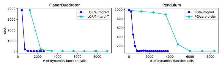
Figure 1: Speedups obtained through differentiable dynamics in two classic settings. Left: In model-based planning, linearizations of dynamics can be computed without finite differences. Right: In model-free policy optimization, the policy gradient can be evaluated directly rather than by a Monte Carlo estimator.

Simulation wall-clock time.

To illustrate the potential for end-to-end performance gains from a purely computational (as opposed to statistical) perspective, we perform a simple comparison of the running times of the classic_control.PendulumEnv environment provided by Gym, and our replica implementation in Deluca. We timed the initial start-up times, then the simulations over $T=10^{7}$ time steps, with all inputs $u_{t}=0$ (to isolate the end-to-end computation time of the dynamics only). The results are shown in Table 1: at the cost of a one-time just-in-time compilation of the dynamics, performed once at the instantiation of the environment, the improvement in the per-iteration time is $>\!1000\times$. This improvement arises from compiler optimizations of functional loops (via jax.lax.scan).

	startup time	time per iteration
Gym (NumPy)	$<1$ $\mu\mathrm{s}$	$54.0\pm 0.2$ $\mu\mathrm{s}$
Deluca (Jax)	$203.0\pm 7.4$ ms	$38.0\pm 4.2$ ns

Table 1: Wall-clock time comparison for simulation of the inverted pendulum. JIT compilation of dynamics, while incurring start-up cost, enables significantly faster simulation. Standard deviations over $100$ runs.

4 Use cases and examples

Motivated by the rise of new gradient-based control methods, and in parallel new applications that exploit them, we survey a few recent developments that highlight the need for the library we propose.

Ventilator control and simulator

Consider the problem of controlling a medical ventilator for pressure-controlled ventilation. The goal is to control airflow in and out of a patient’s lung according to a trajectory of airway pressures specified by a clinician. PID controllers, either hand-tuned or using lung-breath simulators based on gas dynamics, comprise the industry standard for ventilators. In [29], the authors propose a new data-driven methodology to tackle this problem. First, a deep learning based differentiable simulator was trained on exploratory data, which in turn was used to learn a deep controller. Training the controller crucially made use of auto-differentiation. In the absence of a differentiable simulator, accounting for hyperparameter optimization, the pipeline would have taken orders of magnitude more data and compute resources. The figures below are taken from [29].

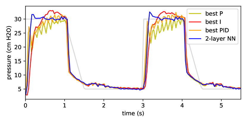
Figure 2: Comparison of a learned controller with hand-tuned PID baselines on the ventilation task.

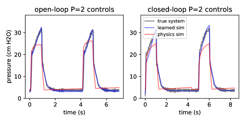
Figure 3: Comparison of learned vs. physics-based simulators on open and closed loop controls.

Adaptive control for the inverted pendulum

Recent advances in online adaptive control give rise to algorithms with provable guarantees even for time-varying linear dynamical systems [13]. These new methods are inherently gradient-based, and differentiate through the dynamics. In figure 4, AdaGPC is compared against the planning algorithm iLQR. Both algorithms require the dynamics’ derivatives so that our library makes their applicability immediate. Furthermore, our library enables experimentation with noise type variations, such as the midway sinusoidal shock in the rightmost plot. We believe studying the trade-offs between planning and online control, as well as the ways to combine the two approaches, is an important new research question that our library helps tackle.

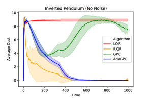
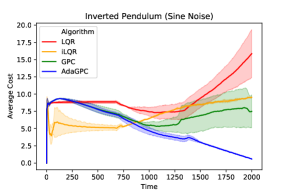
Figure 4: LQR, GPC, iLQR, AdaGPC on inverted pendulum – no noise (left), midway sinusoidal shock (right).

Linear-quadratic control with adversarial perturbations

The inspiration for this library stems from a recent development in control: gradient-based methods that incorporate error feedback into cost functions. The case of linear dynamical systems (LDS) is particularly compelling, as the new methods come with provable guarantees [1, 16, 27]. Our library comes with these new methods pre-implemented, as well as classical control paradigms such as LQR [20] and $\mathcal{H}_{\infty}$ control [38].

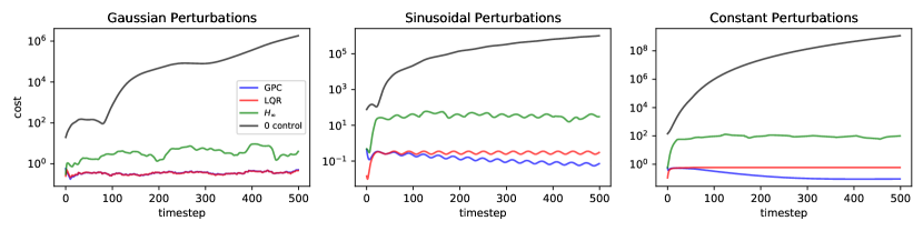
Figure 5: Cost of GPC, LQR and $\mathcal{H}_{\infty}$ control against Gaussian, sinusoidal, and fixed constant perturbations.

Appendix A deluca library details

A.1 Environments

Below is a table of currently supported environments in deluca. We will continue to add to this list.

Environment Obs. Space Act. Space Description classic/acrobot Box(6,) Discrete(2) OpenAI Gym Acrobot-v1 classic/cartpole Box(4,) Discrete(2) OpenAI Gym Cartpole-v1 classic/mountain_car Box(2,) Box(1,) OpenAI Gym MountainCarContinuous-v0 classic/pendulum Box(3,) Box(1,) OpenAI Gym Pendulum-v0 classic/planar_quadrotor Box(6,) Box(2,) Quadrotor in 2D space lds Box(n,) Box(m,) Linear Dynamical System lung/balloon_lung Box(1,) Box(2,) Physics-based lung lung/delay_lung Box(1,) Box(2,) Physics-based lung lung/learned_lung Box(1,) Box(2,) Learned lung

A.2 Agents

Below we give a list of the Agents currently available in the library:

• Adaptive: a general adaptive controller that can turn any suitable base controller into its adaptive counterpart.

• Deep: a generic fully-connected neural-network controller, to be used as a starting-point for more advanced and specific architectures.

• DRC: the recently developed direct response controller [27] for partially observable linear dynamical systems.

• GPC: the gradient perturbation controller [1, 15].

• $\mathbf{H_{\infty}}$: the $H_{\infty}$ robust controller [38].

• iLQR: the iterative linear quadratic regulator, following the approach described in [32].

• LQR: the infinite-horizon, discrete-time linear quadratic regulator [17].

• PID: the proportional-integral-derivative action controller [3].

• PG: Controllers trained via deterministic Policy Gradient.

A.3 Benchmarking

We currently provide a general-purpose benchmarking tool modeled after pytest’s parametrized fixtures and test functions. This tool allows for parallelized experiments to report results across arbitrary arguments (e.g., environments, agents, parameters). We plan to develop more specific benchmarking suites for various classes of environments and agents.

References

- [1] Naman Agarwal, Brian Bullins, Elad Hazan, Sham Kakade, and Karan Singh. Online control with adversarial disturbances. In International Conference on Machine Learning, pages 111–119, 2019.
- [2] VM Aleksandrov, VI Sysoev, and VV Shemeneva. Stochastic optimization of systems. Izv. Akad. Nauk SSSR, Tekh. Kibernetika, pages 14–19, 1968.
- [3] Karl J. Astrom and Tore Hagglung. PID Controllers: Theory, Design and Tuning, 2nd Edition. Instrument Society of America, USA, 1995.
- [4] Dimitri P. Bertsekas. Dynamic Programming and Optimal Control, volume I. Athena Scientific, Belmont, MA, USA, 4th edition, 2017.
- [5] James Bradbury, Roy Frostig, Peter Hawkins, Matthew James Johnson, Chris Leary, Dougal Maclaurin, and Skye Wanderman-Milne. JAX: composable transformations of Python+NumPy programs, 2018.
- [6] Greg Brockman, Vicki Cheung, Ludwig Pettersson, Jonas Schneider, John Schulman, Jie Tang, and Wojciech Zaremba. Openai gym. arXiv preprint arXiv:1606.01540, 2016.
- [7] Xinyi Chen and Elad Hazan. Black-box control for linear dynamical systems. arXiv preprint arXiv:2007.06650, 2020.
- [8] Erwin Coumans et al. Bullet physics library. Open source: bulletphysics. org, 15(49):5, 2013.
- [9] Filipe de Avila Belbute-Peres, Kevin Smith, Kelsey Allen, Josh Tenenbaum, and J Zico Kolter. End-to-end differentiable physics for learning and control. In Advances in Neural Information Processing Systems, pages 7178–7189, 2018.
- [10] Jonas Degrave, Michiel Hermans, Joni Dambre, et al. A differentiable physics engine for deep learning in robotics. Frontiers in neurorobotics, 13:6, 2019.
- [11] Abraham D Flaxman, Adam Tauman Kalai, and H Brendan McMahan. Online convex optimization in the bandit setting: gradient descent without a gradient. In Proceedings of the sixteenth annual ACM-SIAM symposium on Discrete algorithms, pages 385–394, 2005.
- [12] Peter W Glynn. Likelilood ratio gradient estimation: an overview. In Proceedings of the 19th conference on Winter simulation, pages 366–375, 1987.
- [13] Paula Gradu, Elad Hazan, and Edgar Minasyan. Adaptive regret for control of time-varying dynamics. arXiv preprint arXiv:2007.04393, 2020.
- [14] Elad Hazan. Introduction to online convex optimization. Foundations and Trends® in Optimization, 2(3-4):157–325, 2016.
- [15] Elad Hazan, Amit Agarwal, and Satyen Kale. Logarithmic regret algorithms for online convex optimization. Machine Learning, 69(2-3):169–192, 2007.
- [16] Elad Hazan, Sham Kakade, and Karan Singh. The nonstochastic control problem. In Algorithmic Learning Theory, pages 408–421, 2020.
- [17] BL Ho and Rudolf E Kálmán. Effective construction of linear state-variable models from input/output functions. at-Automatisierungstechnik, 14(1-12):545–548, 1966.
- [18] Yuanming Hu, Luke Anderson, Tzu-Mao Li, Qi Sun, Nathan Carr, Jonathan Ragan-Kelley, and Frédo Durand. Difftaichi: Differentiable programming for physical simulation. arXiv preprint arXiv:1910.00935, 2019.
- [19] Yuanming Hu, Jiancheng Liu, Andrew Spielberg, Joshua B Tenenbaum, William T Freeman, Jiajun Wu, Daniela Rus, and Wojciech Matusik. Chainqueen: A real-time differentiable physical simulator for soft robotics. In 2019 International Conference on Robotics and Automation (ICRA), pages 6265–6271. IEEE, 2019.
- [20] Rudolph Emil Kalman. A new approach to linear filtering and prediction problems. Journal of Basic Engineering, 82.1:35–45, 1960.
- [21] David Mayne. A second-order gradient method for determining optimal trajectories of non-linear discrete-time systems. International Journal of Control, 3(1):85–95, 1966.
- [22] David Q Mayne. Model predictive control: Recent developments and future promise. Automatica, 50(12):2967–2986, 2014.
- [23] Volodymyr Mnih, Koray Kavukcuoglu, David Silver, Andrei A Rusu, Joel Veness, Marc G Bellemare, Alex Graves, Martin Riedmiller, Andreas K Fidjeland, Georg Ostrovski, et al. Human-level control through deep reinforcement learning. nature, 518(7540):529–533, 2015.
- [24] John Schulman, Sergey Levine, Pieter Abbeel, Michael Jordan, and Philipp Moritz. Trust region policy optimization. In International conference on machine learning, pages 1889–1897, 2015.
- [25] John Schulman, Filip Wolski, Prafulla Dhariwal, Alec Radford, and Oleg Klimov. Proximal policy optimization algorithms. arXiv preprint arXiv:1707.06347, 2017.
- [26] David Silver, Aja Huang, Chris J Maddison, Arthur Guez, Laurent Sifre, George Van Den Driessche, Julian Schrittwieser, Ioannis Antonoglou, Veda Panneershelvam, Marc Lanctot, et al. Mastering the game of go with deep neural networks and tree search. nature, 529(7587):484–489, 2016.
- [27] Max Simchowitz, Karan Singh, and Elad Hazan. Deluca – a differentiable control library:environments, methods, and benchmarking, 2020.
- [28] Robert F Stengel. Optimal control and estimation. Courier Corporation, 1994.
- [29] Daniel Suo, Udaya Ghai, Edgar Minasyan, Paula Gradu, Xinyi Chen, Naman Agarwal, , Cyril Zhang, Karan Singh, Julienne LaChance, Tom Zajdel, Manuel Schottdorf, Daniel Cohen, and Elad Hazan. Machine learning for medical ventilator control. Manuscript submitted for publication, 2020.
- [30] Richard S Sutton and Andrew G Barto. Reinforcement learning: An introduction. MIT press, 2018.
- [31] Yuval Tassa, Yotam Doron, Alistair Muldal, Tom Erez, Yazhe Li, Diego de Las Casas, David Budden, Abbas Abdolmaleki, Josh Merel, Andrew Lefrancq, et al. Deepmind control suite. arXiv preprint arXiv:1801.00690, 2018.
- [32] Yuval Tassa, Tom Erez, and Emanuel Todorov. Synthesis and stabilization of complex behaviors through online trajectory optimization. In 2012 IEEE/RSJ International Conference on Intelligent Robots and Systems, pages 4906–4913, 2012.
- [33] Russ Tedrake. Underactuated Robotics: Algorithms for Walking, Running, Swimming, Flying, and Manipulation (Course Notes for MIT 6.832). 2020.
- [34] Russ Tedrake and the Drake Development Team. Drake: Model-based design and verification for robotics, 2019.
- [35] Emanuel Todorov, Tom Erez, and Yuval Tassa. Mujoco: A physics engine for model-based control. In 2012 IEEE/RSJ International Conference on Intelligent Robots and Systems, pages 5026–5033. IEEE, 2012.
- [36] Emanuel Todorov and Weiwei Li. A generalized iterative lqg method for locally-optimal feedback control of constrained nonlinear stochastic systems. In Proceedings of the 2005, American Control Conference, 2005., pages 300–306. IEEE, 2005.
- [37] Ronald J Williams. Simple statistical gradient-following algorithms for connectionist reinforcement learning. Machine learning, 8(3-4):229–256, 1992.
- [38] Kemin Zhou, John C. Doyle, and Keith Glover. Robust and Optimal Control. Prentice-Hall, Inc., USA, 1996.