Fast and Accurate Uncertainty Quantification for the ECG with Random Electrodes Location

Abstract

The standard electrocardiogram (ECG) is a point-wise evaluation of the body potential at certain given locations. These locations are subject to uncertainty and may vary from patient to patient or even for a single patient. In this work, we estimate the uncertainty in the ECG induced by uncertain electrode positions when the ECG is derived from the forward bidomain model. In order to avoid the high computational cost associated to the solution of the bidomain model in the entire torso, we propose a low-rank approach to solve the uncertainty quantification (UQ) problem. More precisely, we exploit the sparsity of the ECG and the lead field theory to translate it into a set of deterministic, time-independent problems, whose solution is eventually used to evaluate expectation and covariance of the ECG. We assess the approach with numerical experiments in a simple geometry.

1 Introduction

The standard ECG is a routinely acquired recording of the torso electric potential [14]. It provides valuable information on the electric activity of the heart and, when combined with imaging data of the anatomy, it can be used for non-invasive personalization of sophisticated patient-specific models [10, 17]. In these inverse ECG models, the ECG is rarely computed from the state-of-the-art bidomain model [6], otherwise the computational cost would be prohibitive. Commonly, the bidomain model is replaced by a “decoupled” version, called forward bidomain [19] or pseudo-bidomain [3, 15] model, in which the transmembrane potential in the heart is computed independently from the extracellular potential in the torso. The resulting model still compares favourably to the coupled bidomain model and, more importantly, the ECG can be evaluated very efficiently and exactly by employing the lead field theory [16, 18].

Obviously, when dealing with real data, as in patient-specific modeling, model parameters are subject to unavoidable uncertainty. This uncertainty should be accounted for in the forward and inverse ECG model [5]. Several sources of uncertainty may be considered, e.g., related to the segmentation process of the anatomy [7], the electric conductivities [1], or the fiber distribution [20]. Particularly relevant in the context of inverse ECG modeling is the uncertainty in the electrodes’ locations, which has shown to yield sensible morphological changes in the precordial signals even with a displacement as low as $2\text{\,}\mathrm{cm}$ [13].

The present work focuses on the problem of estimating the expectation and the covariance of the surface ECG, if electrodes’ locations are subject to uncertainty and the ECG is simulated with the forward bidomain model. In principle, given the torso potential, the statistical moments are readily available with little additional cost, as the solution of the UQ problem amounts to a simple integration over the torso domain. In spite of its simplicity, the computational cost of this approach grows linearly with the number of time steps and the number of evaluations of the forward model. Moreover, it relies on the full torso potential, despite the fact that the electrodes’ locations may be very localized. We propose a computationally very efficient methodology to solve the UQ problem without the need of solving the full forward problem. Our method is still based on the lead field theory and it is an exact representation of the true ECG. Specifically, it exploits a low-rank approach to decouple the correlation problem into a small set of elliptic problems for different right hand sides [12]. Remarkably, the overall computational cost is drastically reduced and comparable to the solution of a few elliptic problems, independently of the number of time steps and forward evaluations.

This paper is organized as follows: in Sec. 2, we review the forward bidomain model for the ECG, the lead field approach and describe our method. In Sec. 3, we validate the approach on a simple geometry. We conclude in Sec. 4 with a brief discussion and outlook.

2 Methods

2.1 The forward bidomain model

The electric potential $u_{0}(\mathbf{x},t)$ in the torso $\Omega_{\mathrm{T}}\subset\mathbb{R}^{d}$, and consequently the ECG, can be modelled from the transmembrane potential $V_{\mathrm{m}}(\mathbf{x},t)$ in the active myocardium $\Omega_{\mathrm{H}}\subset\mathbb{R}^{d}$, with the time-dependent forward bidomain model [19], which reads as follows:

$$\begin{cases}-\nabla\cdot\bigl{(}(\mathbf{G}_{\mathrm{i}}+\mathbf{G}_{\mathrm{e}})\nabla u_{\mathrm{e}}(\mathbf{x},t)\bigr{)}=\nabla\cdot(\mathbf{G}_{\mathrm{i}}\nabla V_{\mathrm{m}}(\mathbf{x},t)),&\mbox{in $\Omega_{\mathrm{H}}\times[0,\infty)$},\\ -\nabla\cdot(\mathbf{G}_{0}\nabla u_{0}(\mathbf{x},t))=0,&\mbox{in $\Omega_{\mathrm{T}}\times[0,\infty)$},\\ -\mathbf{G}_{0}\nabla u_{0}(\mathbf{x},t)\cdot\mathbf{n}=0,&\mbox{on $\Sigma\times[0,\infty)$},\\ \phantom{-}u_{\mathrm{e}}(\mathbf{x},t)=u_{0}(\mathbf{x},t),&\mbox{on $\Gamma\times[0,\infty)$},\\ -\mathbf{G}_{\mathrm{b}}\nabla u_{\mathrm{e}}(\mathbf{x},t)\cdot\mathbf{n}+\mathbf{G}_{0}\nabla u_{0}(\mathbf{x},t)\cdot\mathbf{n}=\mathbf{G}_{\mathrm{i}}\nabla V_{\mathrm{m}}(\mathbf{x},t)\cdot\mathbf{n},&\mbox{on $\Gamma\times[0,\infty)$}.\end{cases}$$ (1)

Herein, $\Gamma=\bar{\Omega}_{\mathrm{H}}\cap\bar{\Omega}_{\mathrm{T}}$ is the heart-torso interface, $\Sigma=\partial\Omega_{\mathrm{T}}\setminus\Gamma$ is the body surface, $u_{\mathrm{e}}(\mathbf{x},t)$ is the extra-cellular potential in the heart, $\mathbf{G}_{\mathrm{i}}$ and $\mathbf{G}_{\mathrm{e}}$ are respectively intra- and extra-cellular conductivity of the heart, $\mathbf{G}_{0}$ is the torso conductivity, and $\mathbf{n}$ is the outward normal for both $\Gamma$ and $\Sigma$. For the sake of simplicity in the notation, we define

$$\mathbf{G}\coloneqq\begin{cases}\mathbf{G}_{\mathrm{i}}+\mathbf{G}_{\mathrm{e}}&\text{in }\Omega_{\mathrm{H}},\\ \mathbf{G}_{0}&\text{in }\Omega_{\mathrm{T}},\end{cases}\quad u(\mathbf{x},t)\coloneqq\begin{cases}u_{\mathrm{e}}(\mathbf{x},t)&\text{in }\Omega_{\mathrm{H}},\\ u_{0}(\mathbf{x},t)&\text{in }\Omega_{\mathrm{T}},\end{cases}$$

and assume, without loss of generality, that $u(\cdot,t)\in\mathrm{H}^{1}(\Omega)$, where $\Omega=\Omega_{\mathrm{H}}\cup\Omega_{\mathrm{T}}$. In this case, the variational formulation for Eq. (1) can be written according to

For every $$t\in\mathbb{R} u(\cdot,t)\in\mathrm{H}^{1}(\Omega)$$, find such that (2)

$$\quad\int_{\Omega}\mathbf{G}\nabla u(\mathbf{x},t)\cdot\nabla v\>\mathrm{d}\mathbf{x}=-\int_{\Omega_{\mathrm{H}}}\mathbf{G}_{\mathrm{i}}\nabla V_{\mathrm{m}}(\mathbf{x},t)\cdot\nabla v\>\mathrm{d}\mathbf{x}$$

for all $v\in\mathrm{H}^{1}(\Omega)$. The well-posedness of the problem follows from standard application of the Riesz Theorem [9], given that $\Omega_{\mathrm{H}},\Omega_{\mathrm{T}}$ are Lipschitz domains and $V_{\mathrm{m}}(\cdot,t)\in\mathrm{H}^{1}(\Omega_{\mathrm{H}})$. We remark that the formulation in Eq. (2) is equivalent to Eq. (1) when the restriction of the solution $u|_{\Omega_{i}}$ belongs to $\mathrm{H}^{2}(\Omega_{i})$, $i\in\{\text{H},\text{T}\}$, see e.g. [2, 4] for a more comprehensive treatment of interface problems.

The ECG is a set of so-called leads, typically 12 in the standard ECG. Each lead reads as follows:

$$V(t,{\bm{\xi}}_{1},\ldots,{\bm{\xi}}_{L})=\sum_{\ell=1}^{L}a_{\ell}u({\bm{\xi}}_{\ell},t),$$ (3)

where ${\bm{\Xi}}\coloneqq\{{\bm{\xi}}_{\ell}\}_{\ell=1}^{L}$ is the set of electrodes and $\mathbf{a}=[a_{1},\ldots,a_{L}]^{\top}$ is a zero-sum vector of weights defining the lead. For instance, a limb lead is the potential difference of 2 electrodes, whereas a precordial lead involves 4 electrodes (3 are used to build the Wilson Central Terminal, that is the reference potential). It is worth noting that Eq. (3) is valid only if $u(\cdot,t)\in\mathcal{C}^{0}(\Sigma)$, which is not true for $u(\cdot,t)\in\mathrm{H}^{1}(\Omega)$ and $d\geq 2$. For a rigorous discussion, see [6].

In this work, we are interested in computing statistics of $V\big{(}t,{\bm{\Xi}}(\omega)\big{)}$ when the electrode positions ${\bm{\Xi}(\omega)\coloneqq\{{\bm{\xi}}_{\ell}(\omega)\}_{\ell=1}^{L}}$ are not known exactly. Here, we denote by ${\bm{\xi}}_{\ell}(\omega)$ the random variable associated to the $\ell$-th electrode and assume that the joint distribution is given by the density $\rho(\mathbf{X})=\rho(\mathbf{x}_{1},\ldots,\mathbf{x}_{L})$ with respect to the surface measure $\mathrm{d}\sigma_{\mathbf{X}}=\mathrm{d}\sigma_{\mathbf{x}_{1}}\cdots\mathrm{d}\sigma_{\mathbf{x}_{L}}$ on $\Sigma^{L}$. According to the definition in Eq. (3), the lead $V(t,{\bm{\Xi}})$ is a random field as well, with expectation and correlation respectively reading as follows:

$$\mathbb{E}[V](t) =\int_{\Sigma^{M}}V(t,\mathbf{X})\rho(\mathbf{X})\mathrm{d}\sigma_{\mathbf{X}},$$ (4)

$$\operatorname{Cor}[V](t,s) =\int_{\Sigma^{M}}V(t,\mathbf{X})V(s,\mathbf{X})\rho(\mathbf{X})\mathrm{d}\sigma_{\mathbf{X}}.$$ (5)

In summary, the UQ problem for the random electrodes locations consists in solving the forward bidomain model Eq. (1) for $u(\mathbf{x},t)$, given $V_{\mathrm{m}}(\mathbf{x},t)$, for every time $t$, and then computing the integrals in Eq. (4) and Eq. (5).

2.2 Lead field formulation of the UQ problem

Clearly, in general it is not convenient to compute the ECG from Eq. (1), because the ECG is only a very sparse evaluation of $u(\mathbf{x},t)$. Moreover, in a patient-specific or personalization context, the ECG needs to be simulated several times with different instances of $V_{\mathrm{m}}(\mathbf{x},t)$, with no changes in the left hand side of Eq. (1). A better approach is based on Green’s functions, also known as lead fields in the electrocardiographic literature [18]. In fact, it is possible to show that $V(t,{\bm{\Xi}})$ has the following representation [6]:

$$V(t,{\bm{\Xi}})=\int_{\Omega_{\mathrm{H}}}\mathbf{G}_{\mathrm{i}}(\mathbf{x})\nabla V_{\mathrm{m}}(\mathbf{x},t)\cdot\nabla Z(\mathbf{x},{\bm{\Xi}})\>\mathrm{d}{\mathbf{x}},$$ (6)

where $Z(\mathbf{x},{\bm{\Xi}})$ is the weak solution of the elliptic problem:

$$\begin{cases}-\nabla\cdot\mathbf{G}\nabla Z(\mathbf{x},{\bm{\Xi}})=0,&\text{in }\Omega,\\ -\mathbf{G}\nabla Z(\mathbf{x},{\bm{\Xi}})\cdot\mathbf{n}=\sum_{\ell=1}^{L}a_{\ell}\delta_{{\bm{\xi}}_{\ell}},&\text{on }\Sigma,\end{cases}$$ (7)

where $\delta_{{\bm{\xi}}_{\ell}}$ is the $(d-1)$-dimensional Dirac delta centered at ${\bm{\xi}}_{\ell}(\omega)$. Therefore, given that all measurement locations are fixed, Eq. (7) is only solved once, at the cost of a single time step of Eq. (1), and then used to compute $V(t,{\bm{\Xi}})$ for any choice of $V_{\mathrm{m}}(\mathbf{x},t)$.

Here, we exploit Eq. (6) to compute the the expectation and correlation of $V$, according to Eq. (4) and (5). Substituting Eq. (6) into Eq. (4), we obtain by the linearity of the expectation that

$$\mathbb{E}[V](t)=\int_{\Omega_{\mathrm{H}}}\mathbf{G}_{\mathrm{i}}(\mathbf{x})\nabla V_{\mathrm{m}}(\mathbf{x},t)\cdot\nabla\mathbb{E}[Z](\mathbf{x})\>\mathrm{d}{\mathbf{x}}.$$ (8)

Again by linearity, the equation for the expected lead field $\mathbb{E}[Z]$ follows from Eq. (7) and reads as follows:

$$\begin{cases}-\nabla\cdot\mathbf{G}\nabla\mathbb{E}[Z](\mathbf{x})=0,&\text{in }\Omega,\\ -\mathbf{G}\nabla\mathbb{E}[Z](\mathbf{x})\cdot\mathbf{n}=\sum_{\ell=1}^{M}a_{\ell}\rho_{\ell}(\mathbf{x}),&\text{on }\Sigma,\end{cases}$$ (9)

where $\rho_{\ell}$ is the marginal distribution of $\rho$ with respect to ${\bm{\xi}}_{\ell}$, that is

$$\rho_{\ell}(\mathbf{x}_{\ell})\coloneqq\int_{\Sigma^{L-1}}\rho(\mathbf{X})\>\mathrm{d}\sigma_{\mathbf{x}_{1}}\cdots\mathrm{d}\sigma_{\mathbf{x}_{\ell-1}}\mathrm{d}\sigma_{\mathbf{x}_{\ell+1}}\cdots\mathrm{d}\sigma_{\mathbf{x}_{L}}.$$ (10)

To show this, we observe that:

$$\mathbb{E}\biggl{[}\sum_{\ell=1}^{L}a_{\ell}\delta_{{\bm{\xi}}_{\ell}}\biggr{]}=\sum_{i=1}^{L}a_{\ell}\int_{\Sigma^{L}}\delta_{\mathbf{x}_{\ell}}\rho(\mathbf{X})\;\mathrm{d}\sigma_{\mathbf{X}}\\ =\sum_{\ell=1}^{L}a_{\ell}\rho_{\ell}.$$

Therefore, the cost of computing the average ECG is equivalent to that for solving for the point-wise ECG, i.e., one solution of the elliptic problem in Eq. (9). We observe that both Eq. (7) and Eq. (9) are well-posed, since the right hand side has zero average over $\Sigma$ in both cases. In particular, for every $\omega$, $Z(\mathbf{x},{\bm{\Xi}}(\omega))$ and $\mathbb{E}[Z](\mathbf{x})$ are only defined up to a constant.

The natural continuation of the above argument yields the correlation for the ECG according to

$$\operatorname{Cor}[V](t,s)=\int_{\Sigma^{2}}(\mathbf{G}_{\mathrm{i}}\nabla\otimes\mathbf{G}_{\mathrm{i}}\nabla)V_{\mathrm{m}}(\mathbf{x},t)V_{\mathrm{m}}(\mathbf{x}^{\prime},s):(\nabla\otimes\nabla)\operatorname{Cor}[Z]\>\mathrm{d}\sigma_{\mathbf{x}}\mathrm{d}\sigma_{\mathbf{x}^{\prime}},$$

where the tensor product is $[\mathbf{u}\otimes\mathbf{v}]_{ij}=u_{i}(\mathbf{x})v_{j}(\mathbf{x}^{\prime})$ and the inner product between tensors is $\mathbf{A}:\mathbf{B}=\sum_{ij}[A]_{ij}[B]_{ij}$. The problem for the correlation $\operatorname{Cor}[Z]$, obtained as above from Eq. (7), reads as follows:

$$\begin{cases}(\nabla\cdot\mathbf{G}\nabla\otimes\nabla\cdot\mathbf{G}\nabla)\operatorname{Cor}[Z]=0,&\text{in }\Omega\times\Omega,\\ (\mathbf{n}\cdot\mathbf{G}\nabla\otimes\nabla\cdot\mathbf{G}\nabla)\operatorname{Cor}[Z]=0,&\text{on }\Sigma\times\Omega,\\ (\nabla\cdot\mathbf{G}\nabla\otimes\mathbf{n}\cdot\mathbf{G}\nabla)\operatorname{Cor}[Z]=0,&\text{on }\Omega\times\Sigma,\\ (\mathbf{n}\cdot\mathbf{G}\nabla\otimes\mathbf{n}\cdot\mathbf{G}\nabla)\operatorname{Cor}[Z]=R,&\text{on }\Sigma\times\Sigma,\end{cases}$$ (11)

where the correlation $R(\mathbf{x},\mathbf{x}^{\prime})$ of the Neumann data in Eq. (7) is

$$\begin{split}R(\mathbf{x},\mathbf{x}^{\prime})&=\operatorname{Cor}\biggl{[}\sum_{\ell=1}^{L}a_{\ell}\delta_{{\bm{\xi}}_{\ell}},\sum_{\ell^{\prime}=1}^{L}a_{\ell^{\prime}}\delta_{{\bm{\xi}}_{\ell^{\prime}}}\biggr{]}\\ &=\sum_{\ell=1}^{L}a_{\ell}^{2}\rho_{\ell}(\mathbf{x})\delta_{\mathbf{x}}(\mathbf{x}^{\prime})+\sum_{\ell\neq\ell^{\prime}}^{L}a_{\ell}a_{\ell^{\prime}}\rho_{\ell,\ell^{\prime}}(\mathbf{x},\mathbf{x}^{\prime}),\end{split}$$ (12)

with $\rho_{\ell,\ell^{\prime}}(\mathbf{x},\mathbf{x}^{\prime})$ being the marginal distribution of $\rho$ with respect to $(\bm{\xi}_{\ell},\bm{\xi}_{\ell}^{\prime})$ and defined as follows:

$$\rho_{\ell,\ell^{\prime}}(\mathbf{x}_{\ell},\mathbf{x}_{\ell^{\prime}})\coloneqq\int_{\Sigma^{L-2}}\rho(\mathbf{X})\>\mathrm{d}\sigma_{\mathbf{x}_{1}}\cdots\mathrm{d}\sigma_{\mathbf{x}_{\ell-1}}\mathrm{d}\sigma_{\mathbf{x}_{\ell+1}}\cdots\mathrm{d}\sigma_{\mathbf{x}_{\ell^{\prime}-1}}\mathrm{d}\sigma_{\mathbf{x}_{\ell^{\prime}+1}}\cdots\mathrm{d}\sigma_{\mathbf{x}_{L}}.$$ (13)

We observe that, when $\bm{\xi}_{\ell}$ and $\bm{\xi}_{\ell}^{\prime}$ are independent, $\rho_{\ell,\ell^{\prime}}(\mathbf{x}_{\ell},\mathbf{x}_{\ell^{\prime}})$ factorizes into the product of the marginals $\rho_{\ell}(\mathbf{x}_{\ell})$ and $\rho_{\ell^{\prime}}(\mathbf{x}_{\ell^{\prime}})$.

As the computation of $\operatorname{Cor}[Z]$ requires the solution of a tensor product boundary value problem, it is computationally rather expensive. In what follows, we will exploit the particular structure of $R(\mathbf{x},\mathbf{x}^{\prime})$ to significantly reduce the computational cost and implementation effort. We remark that also Eq. (11) is well-posed because, by construction, $R(\mathbf{x},\mathbf{x}^{\prime})$ is such that $\langle R,1\otimes v\rangle_{\Sigma^{2}}=\langle R,v\otimes 1\rangle_{\Sigma^{2}}=0$ for all $v\in\mathrm{H}^{1/2}(\Sigma)$, where $\langle\cdot,\cdot\rangle_{\Sigma^{2}}$ is the duality pairing in $\mathrm{L}^{2}(\Sigma^{2})$.

2.3 Numerical Discretization

The variational formulation of the averaged lead field problem Eq. (8) resembles Eq. (2) with a different right hand side. With $Y=\mathrm{H}^{1}(\Omega)$, the problem is:

Find $$\mathbb{E}[Z]\in Y$$ such that

$$\qquad\int_{\Omega}\mathbf{G}\nabla\mathbb{E}[Z]\cdot\nabla v\>\mathrm{d}\mathbf{x}=\int_{\Sigma}\sum_{\ell=1}^{L}a_{\ell}\rho_{\ell}v\>\mathrm{d}\mathbf{x},\quad\text{for all $v\in Y$}.$$

The Galerkin approximation in the space $Y_{h}\subset Y$, with $Y_{h}=\operatorname{span}\{\phi_{k}\}_{k=1}^{N_{h}}$, reads as follows:

$$\mathbf{K}\mathbf{z}=\mathbf{g},$$ (14)

where $\mathbf{z}$ is the solution vector, that is $\mathbb{E}[Z]\approx Z_{h}=\sum_{k}[\mathbf{z}]_{k}\phi_{k}$ and

$$[\mathbf{K}]_{k\ell} =\int_{\Omega}\mathbf{G}\nabla\phi_{\ell}\cdot\nabla\phi_{k}\>\mathrm{d}\mathbf{x},$$ (15)

$$[\mathbf{g}]_{k} =\int_{\Sigma}\sum_{\ell=1}^{M}a_{\ell}\rho_{\ell}(\mathbf{x})\phi_{k}(\mathbf{x})\>\mathrm{d}\mathbf{x}.$$ (16)

For the correlation in Eq. (11), the variational formulation is as follows:

Find $$\operatorname{Cor}[Z]\in Y\otimes Y$$ such that

$$\qquad\int_{\Omega^{2}}(\mathbf{G}\nabla\otimes\mathbf{G}\nabla)\operatorname{Cor}[Z]:(\nabla\otimes\nabla)v\>\mathrm{d}\mathbf{x}\mathrm{d}\mathbf{x}^{\prime}=\int_{\Sigma^{2}}Rv\>\mathrm{d}\mathbf{x}\mathrm{d}\mathbf{x}^{\prime}$$

for all $v\in Y\otimes Y$. The corresponding Galerkin formulation on $Y_{h}\times Y_{h}$ is:

$$(\mathbf{K}\otimes\mathbf{K})\mathbf{Z}=\mathbf{R},$$ (17)

where $\operatorname{Cor}[Z]\approx\sum_{k,\ell}[\mathbf{Z}]_{k\ell}\phi_{k}\otimes\phi_{\ell}$ and

$$\begin{split}[\mathbf{R}]_{pq}&=\int_{\Sigma^{2}}R\phi_{p}\phi_{q}\mathrm{d}\mathbf{x}\mathrm{d}\mathbf{x}^{\prime}\\ &=\sum_{\ell=1}^{L}a_{\ell}^{2}\int_{\Sigma}\rho_{\ell}\phi_{p}\phi_{q}\mathrm{d}\mathbf{x}+\sum_{\ell\neq\ell^{\prime}}^{L}a_{\ell}a_{\ell^{\prime}}\int_{\Sigma^{2}}\rho_{\ell,\ell^{\prime}}\phi_{p}\phi_{q}\mathrm{d}\mathbf{x}\mathrm{d}\mathbf{x}^{\prime}.\end{split}$$ (18)

As the number of degrees of freedom for the correlation problem is $N_{h}^{2}$, it may easily become computationally prohibitive. However, assuming that the marginal densities $\rho_{\ell}$, $\ell=1,\ldots,L$ are strongly localized, the right hand side in (17) may be represented by a low-rank approximation according to

$$\mathbf{R}\approx\sum_{k=1}^{K}\bm{r}_{k}\otimes\bm{r}_{k},\quad\bm{r}_{k}\in\mathbb{R}^{N_{h}},$$

with $K\ll N_{h}$. In this case, we also expect a low-rank solution, that is

$$\mathbf{Z}\approx\sum_{k=1}^{K}\bm{\zeta}_{k}\otimes\bm{\zeta}_{k},\quad\bm{\zeta}_{k}\in\mathbb{R}^{N_{h}},$$

with $K\ll N_{h}$. Then, due to the tensor product structure of (17), there simply holds

$$\mathbf{K}\bm{\zeta}_{k}=\bm{r}_{k},\qquad k=1,\ldots,K.$$ (19)

In practice, we compute the low-rank approximation by a diagonally pivoted, truncated Cholesky decomposition, see [11].

Finally, for the computation of statistics of the ECG, we insert the computed Galerkin approximations into Eq. (4) and Eq. (5) and obtain

$$\mathbb{E}[V](t) \approx\mathbf{V}(t)\cdot\mathbf{z},$$ (20)

$$\operatorname{Cor}[V](t,s) \approx\sum_{k,m=1}^{K}\big{(}\mathbf{V}(t)\cdot\bm{\zeta}_{k}\big{)}\big{(}\mathbf{V}(s)\cdot\bm{\zeta}_{m}\big{)},$$ (21)

where

$$[\mathbf{V}(t)]_{j}=\int_{\Omega_{\mathrm{H}}}\mathbf{G}_{\mathrm{i}}\nabla V_{\mathrm{m}}(t)\cdot\nabla\phi_{j}\>\mathrm{d}\mathbf{x}.$$

The computational cost for the proposed approach is dominated by the solution of $K+1$ systems (one for the expectation and $K$ for the correlation) of the form of Eq. (14). It is therefore independent on the number of time steps $N_{t}$ or the choice of $V_{\mathrm{m}}$, oppositely to the solution of the forward bidomain model in Eq. (1), which requires $K\cdot N_{t}$ solutions for each choice of $V_{\mathrm{m}}$.

We summarize below the proposed procedure to evaluate expectation and correlation of a single lead of the ECG, defined with $L\geq 2$ coefficients $\mathbf{a}$ as in Eq. (6) and with random electrodes locations $\{\bm{\xi}_{\ell}\}_{\ell=1}^{L}$ with density $\rho(\mathbf{X})$. We assume as above that $V_{\mathrm{m}}(\mathbf{x},t)$ is given and computed elsewhere.

1. Compute $\rho_{\ell}(\mathbf{x})$ with Eq. (10) and assemble $\mathbf{g}$ with Eq. (16);

2. Assemble $\mathbf{K}$ with Eq. (15) and solve Eq. (14) to find $\mathbf{z}$;

3. Compute $\mathbb{E}[V](t)$ from $\mathbf{z}$ and $V_{\mathrm{m}}$ with Eq. (20);

4. Compute $\rho_{\ell,\ell^{\prime}}(\mathbf{x},\mathbf{x}^{\prime})$ with Eq. (13) and assemble $\mathbf{R}$ with Eq. (18);

5. Compute the low-rank Cholesky decomposition $\{\bm{r}_{k}\}_{k=1}^{K}$ of $\mathrm{R}$;

6. For each $k=1,\ldots,K$, solve Eq. (19) for $\bm{\zeta}_{k}$;

7. Compute $\operatorname{Cor}[V](t,s)$ from $\{\bm{\zeta}_{k}\}_{k=1}^{K}$ and $V_{\mathrm{m}}$ with Eq. (21).

3 Numerical Assessment

We tested the proposed approach on a idealized heart-torso geometry in 2-D, as depicted in Fig. 1. The anatomy consists of an ellipsoidal torso with major semi-axis of $T_{y}=$15\text{\,}\mathrm{cm}$$, vertically oriented, and minor axis of $T_{x}=$10\text{\,}\mathrm{cm}$$. The heart was an annulus centered at $\mathbf{x}_{\mathrm{h}}=($-4\text{\,}\mathrm{cm}$,$2\text{\,}\mathrm{cm}$)$ with respect to the center of the torso, and with inner (endocardium) and outer (epicardium) radius respectively equal to $2\text{\,}\mathrm{cm}$ and $3\text{\,}\mathrm{cm}$. The domain was split into 3 distinct regions, namely blood pool, myocardium and torso (see Fig. 1).

For this test, we considered an ECG with 2 leads obtained from 4 random electrodes $\bm{\xi}_{\ell}(\omega)$, $\ell=\{\mathrm{VL},\mathrm{VR},\mathrm{VF},\mathrm{V1}\}$, see Fig. 1. The leads, II and V1, were

$$V_{\mathrm{II}}(t,\bm{\Xi}) =u(\bm{\xi}_{\mathrm{VF}},t)-u(\bm{\xi}_{\mathrm{VL}},t),$$

$$V_{\mathrm{V1}}(t,\bm{\Xi}) =u(\bm{\xi}_{\mathrm{V1}},t)-\frac{1}{3}\Bigl{(}u(\bm{\xi}_{\mathrm{VL}},t)+u(\bm{\xi}_{\mathrm{VR}},t)+u(\bm{\xi}_{\mathrm{VF}},t)\Bigr{)},$$

respectively corresponding to $\mathbf{a}_{\mathrm{II}}=(-1,0,1,0)$ and $\mathbf{a}_{\mathrm{V1}}=(-\frac{1}{3},-\frac{1}{3},-\frac{1}{3},1)$. The average position $\mathbf{x}_{\ell}$ of the electrodes was conveniently defined using the formula $\mathbf{x}_{\ell}=[T_{x}\cos(\theta_{\ell}),T_{y}\sin(\theta_{\ell})]^{\top}$ with $\theta_{\mathrm{VL}}=\frac{3}{4}\pi$, $\theta_{\mathrm{VR}}=\frac{1}{4}\pi$, $\theta_{\mathrm{VF}}=\frac{3}{2}\pi$ and $\theta_{\mathrm{V1}}=\pi$.

In all tests, we evaluated the deterministic ECG, computed from Eq. (6), the average ECG when electrodes were randomly located, and the variance from the formula $\operatorname{Var}[V](t)=\operatorname{Cor}[V](t,t)-\big{(}\mathbb{E}[V](t)\big{)}^{2}$.

The random electrode locations, independent from each other, were either uniformly distributed or with a Gaussian-like distribution, both defined on the outer boundary $\Sigma$ of the torso (the “chest”), see Fig. 1. In the case of the uniform distribution, the marginal density $\rho_{\ell}$ for each electrode was the characteristic function of the set $\Sigma_{\ell}=\{\mathbf{x}\in\Sigma:d(\mathbf{x}_{\ell},\mathbf{x})\leq r_{\ell}\}$, that is the $r_{\ell}$-neighborhood of $\mathbf{x}_{\ell}$ with respect to the geodesic distance $d$ on the curve $\Sigma$. We also considered a Gaussian-like distribution computed, after a normalization, by solving the heat equation on the boundary curve $\Sigma$ with diffusion defined along the arc-length, initial datum $\delta(\mathbf{x}-\mathbf{x}_{\ell})$ on $\Sigma$, and solved for a total time $T_{\ell}$, see Fig. 1. We selected $r_{\ell}=$1.5\text{\,}\mathrm{cm}$$ and $T_{\ell}=\sqrt{3}/3r_{\ell}$, so that both distributions have the same variance.

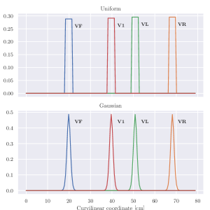
Figure 1: Geometrical configuration for the numerical test. On the left, the domain is represented with electrodes locations on the boundary and tissue properties. On the right, the probability density function for both uniform and Gaussian-like cases is reported. The $x$-axis is the curvilinear coordinate, and colors of the curves refer to the electrodes on the left.

For convenience, we report the full expression $R(\mathbf{x},\mathbf{x}^{\prime})$ for lead II, obtained by assuming that $\bm{\xi}_{\mathrm{VF}}$ and $\bm{\xi}_{\mathrm{VL}}$ were independent:

$$R(\mathbf{x},\mathbf{x}^{\prime})=\bigl{(}\rho_{\mathrm{VF}}(\mathbf{x})+\rho_{\mathrm{VL}}(\mathbf{x})\bigr{)}\delta_{\mathbf{x}}(\mathbf{x}^{\prime})-\rho_{\mathrm{VF}}(\mathbf{x})\rho_{\mathrm{VL}}(\mathbf{x}^{\prime})-\rho_{\mathrm{VL}}(\mathbf{x})\rho_{\mathrm{VF}}(\mathbf{x}^{\prime}).$$

In particular, the assembly of the tensor $\mathbf{R}$ simplifies as well, with no need of evaluating a double integral. In fact,

$$[\mathbf{R}]_{pq}=\int_{\Sigma}\bigl{(}\rho_{\mathrm{VF}}+\rho_{\mathrm{VL}}\bigr{)}\bigl{(}\phi_{p}\phi_{q}-\phi_{p}-\phi_{q}\bigr{)}\mathrm{d}\sigma_{\mathbf{x}}.$$

The electric conductivities were uniform and isotropic in the torso and in the blood pool, and respectively set to $2\text{\,}\mathrm{mS}\text{\,}{\mathrm{cm}}^{-1}\text{\,}{\mathrm{}}^{2}$ and $6\text{\,}\mathrm{mS}\text{\,}{\mathrm{cm}}^{-1}\text{\,}{\mathrm{}}^{2}$. The myocardium was assumed transversely isotropic, with fibers $\mathbf{f}$ circularly oriented and of unit length. Specifically:

$$\mathbf{G}_{\mathrm{i}} =\sigma_{\mathrm{i},\mathrm{t}}\mathbf{I}+(\sigma_{\mathrm{i},\mathrm{l}}-\sigma_{\mathrm{i},\mathrm{t}})\mathbf{f}\otimes\mathbf{f},$$

$$\mathbf{G}_{\mathrm{e}} =\sigma_{\mathrm{e},\mathrm{t}}\mathbf{I}+(\sigma_{\mathrm{e},\mathrm{l}}-\sigma_{\mathrm{e},\mathrm{t}})\mathbf{f}\otimes\mathbf{f},$$

and values set to $\sigma_{\mathrm{i},\mathrm{l}}=$3\text{\,}\mathrm{mS}\text{\,}{\mathrm{cm}}^{-1}\text{\,}{\mathrm{}}^{2}$$, $\sigma_{\mathrm{i},\mathrm{t}}=$0.3\text{\,}\mathrm{mS}\text{\,}{\mathrm{cm}}^{-1}\text{\,}{\mathrm{}}^{2}$$, $\sigma_{\mathrm{e},\mathrm{l}}=$3\text{\,}\mathrm{mS}\text{\,}{\mathrm{cm}}^{-1}\text{\,}{\mathrm{}}^{2}$$ and $\sigma_{\mathrm{e},\mathrm{t}}=$1.2\text{\,}\mathrm{mS}\text{\,}{\mathrm{cm}}^{-1}\text{\,}{\mathrm{}}^{2}$$.

Figure 2: On the left (panel A), the activation map computed with the eikonal solution, in $\mathrm{ms}$. On right, lead fields (in $\mathrm{mV}$) for the average problem are reported for lead II (panel B) and lead V1 (panel C).

For sake of simplicity, the transmembrane potential $V_{\mathrm{m}}(\mathbf{x},t)$ was modelled by shifting a fixed action potential template at given activation times $\tau(\mathbf{x})$, according to the formula

$$V_{\mathrm{m}}(\mathbf{x},t)=U\bigl{(}t-\tau(\mathbf{x})\bigr{)},\qquad U(s)=V_{\mathrm{rest}}+\frac{V_{\mathrm{dep}}-V_{\mathrm{rest}}}{2}\biggl{(}1+\tanh\Bigl{(}\frac{s}{\varepsilon}\Bigr{)}\biggr{)}.$$

The activation map $\tau\colon\Omega_{\mathrm{H}}\to\mathbb{R}$ was simulated with the eikonal model

$$\begin{cases}\sqrt{\mathbf{D}(\mathbf{x})\nabla\tau\cdot\nabla\tau}=1,&\mathbf{x}\in\Omega_{\mathrm{H}}\setminus\{\mathbf{x}_{\mathrm{s}}\},\\ \tau(\mathbf{x}_{\mathrm{s}})=0.&\end{cases}$$

The conductivity tensor was set proportional to the monodomain conductivity and such to yield a conduction velocity along the fibers of $65\text{\,}\mathrm{cm}\text{\,}{\mathrm{s}}^{-1}$, that is,

$$\mathbf{D}=\alpha\cdot\mathbf{G}_{\mathrm{m}},$$

where $\mathbf{G}_{\mathrm{m}}=\mathbf{G}_{\mathrm{i}}(\mathbf{G}_{\mathrm{i}}+\mathbf{G}_{\mathrm{e}})^{-1}\mathbf{G}_{\mathrm{e}}$ and $\alpha\approx$2.82\text{\times}{10}^{-3}\text{\,}{\mathrm{cm}}^{4}\text{\,}{\mathrm{ms}}^{2}\text{\,}{\mathrm{mS}}^{-1}$$. The other parameters were as follows: $V_{\mathrm{rest}}=$-85\text{\,}\mathrm{mV}$$, $V_{\mathrm{dep}}=$30\text{\,}\mathrm{mV}$$, $\varepsilon=$0.4\text{\,}\mathrm{ms}$$, and $\mathbf{x}_{\mathrm{s}}=(-$2\text{\,}\mathrm{cm}$,$2\text{\,}\mathrm{cm}$)$.

The computational domain was approximated by a triangular mesh $\mathcal{T}_{h}$ with median edge size of $0.04\text{\,}\mathrm{cm}$ in $\Omega_{\mathrm{H}}$ and $0.5\text{\,}\mathrm{cm}$ in the rest of the domain, thus totalling $27\,820$ nodes and $55\,476$ cells. All quantities were represented by linear finite elements on $\mathcal{T}_{h}$. The eikonal equation was solved with an anisotropic version of the heat distance method [8], with $\Delta t=$4\text{\,}\mathrm{ms}$$. The implementation in FEniCS is publicly available and complemented with additional tests and comparison to the monodomain and bidomain models.

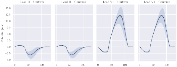
Figure 3: ECG results for all tests. In the plots, the dashed black curve is the deterministic ECG, the solid blue curve is the average ECG, and the shaded blue area corresponds to the $95\text{\,}\mathrm{\char 37\relax}$ confidence interval, that is $\mathbb{E}[V](t)\pm 1.96\sqrt{\operatorname{Var}[V](t)}$.

The activation map and the average lead fields for lead II and lead V1, as computed from Eq. (8), are reported in Fig. 2. In the correlation problem, the low-rank representation counted 17 (resp. 33) modes for lead II with uniform (resp. Gaussian) distribution of electrodes, and 33 (resp. 59) modes for lead V1. A lower number of modes for the uniform distribution was expected, as its support was compact and highly localized. The resulting ECGs are reported in Fig. 3. In both leads, the deterministic and average ECGs were very close, with an absolute error between $0.083\text{\,}\mathrm{mV}$ (lead II) and $0.28\text{\,}\mathrm{mV}$ (lead V1). The uncertainty was significantly higher in the late part of the QRS-complex. Maximum standard deviation was as high as $2.07\text{\,}\mathrm{mV}$ in lead V1 and $0.83\text{\,}\mathrm{mV}$ in lead II. In lead V1, the morphological variations were limited but the maximum amplitude changed significantly. In lead II, morphological differences were present in the second half of the ECG. No appreciable differences in ECGs were noted when comparing uniform and Gaussian-like distributions.

Finally, we compared the proposed method against the solution of the forward bidomain model, see Fig. 4. Differences between ECGs computed from our approach were essentially matching those derived from the forward bidomain model, with an absolute error less than $0.01\text{\,}\mathrm{mV}$ in all cases and quantities of interests. The total cost of the forward simulation was from 2 to 8-fold higher than the lead field approach.

Figure 4: Excerpt of extracellular potential (in $\mathrm{mV}$) of the forward bidomain simulation.

4 Discussion and Conclusions

In this work, we have solved the problem of quantifying the uncertainty in the ECG when uncertainty in the electrode positions is taken into account. Our method recasts the problem into a fully deterministic setting by using the lead field theory and a low-rank approximation for the correlation.

The computational advantage is significant over the standard forward simulation of the bidomain model. In fact, the number of lead fields to be computed in the proposed approach, for both the expectation and the correlation, does not depend on neither the transmembrane potential nor time, oppositely to the bidomain model. The method is therefore suitable to compute ECGs for long simulations, e.g., arrhythmic events, and it is even more advantageous in the context of inverse ECG approaches. Finally, the lead fields are smoother than the extracellular potential, especially within the heart, where potential gradients are strong along the activation front. A much coarser resolution may be employed for computing the lead fields, with no significant loss in accuracy [18].

While formulated for the chest electrodes, the presented theory also applies with minimal changes to assess the uncertainty of intracardiac electrogram recordings, widely employed in clinical electrophysiological studies. As a matter of fact, the formulation is flexible enough to address other relevant problems, such as quantifying the uncertainty in the ECG due to, e.g., uncertain transmembrane potential or torso-heart segmentation, hence leading to more robust simulation results.

References

- [1] Aboulaich, R., Fikal, N., El Guarmah, E., Zemzemi, N.: Stochastic finite element method for torso conductivity uncertainties quantification in electrocardiography inverse problem. Math. Model. Nat. Phenom. 11(2), 1–19 (2016)
- [2] Ammari, H., Chen, D., Zou, J.: Well-posedness of an electric interface model and its finite element approximation. Math. Models Methods Appl. Sci. 26(03), 601–625 (2016)
- [3] Bishop, M.J., Plank, G.: Bidomain ECG simulations using an augmented monodomain model for the cardiac source. IEEE Trans. Biomed. Eng. 58(8), 2297–2307 (2011)
- [4] Chen, Z., Zou, J.: Finite element methods and their convergence for elliptic and parabolic interface problems. Numer. Math. 79(2), 175–202 (1998)
- [5] Clayton, R.H., Aboelkassem, Y., Cantwell, C.D., Corrado, C., Delhaas, T., Huberts, W., Lei, C.L., Ni, H., Panfilov, A.V., Roney, C., et al.: An audit of uncertainty in multi-scale cardiac electrophysiology models. Philos. Trans. R. Soc. Lond. A 378(2173), 20190335 (2020)
- [6] Colli Franzone, P., Pavarino, L.F., Scacchi, S.: Mathematical Cardiac Electrophysiology. Springer, Cham (2014)
- [7] Corrado, C., Razeghi, O., Roney, C., Coveney, S., Williams, S., Sim, I., O’Neill, M., Wilkinson, R., Oakley, J., Clayton, R.H., et al.: Quantifying atrial anatomy uncertainty from clinical data and its impact on electro-physiology simulation predictions. Med. Image Anal. 61, 101626 (2020)
- [8] Crane, K., Weischedel, C., Wardetzky, M.: Geodesics in heat: A new approach to computing distance based on heat flow. ACM Trans. Graph. 32(5), 1–11 (2013)
- [9] Evans, L.C.: Partial Differential Equations. American Mathematical Society (2010)
- [10] Giffard-Roisin, S., Delingette, H., Jackson, T., Webb, J., Fovargue, L., Lee, J., Rinaldi, C.A., Razavi, R., Ayache, N., Sermesant, M.: Transfer learning from simulations on a reference anatomy for ECGI in personalized cardiac resynchronization therapy. IEEE. Trans. Biomed. Eng. 66(2), 343–353 (2019)
- [11] Harbrecht, H., Peters, M., Schneider, R.: On the low-rank approximation by the pivoted Cholesky decomposition. Appl. Numer. Math. 62, 28–440 (2012)
- [12] Harbrecht, H., Li, J.: First order second moment analysis for stochastic interface problems based on low-rank approximation. ESAIM: Math. Model. Numer. Anal. 47(5), 1533–1552 (2013)
- [13] Kania, M., Rix, H., Fereniec, M., Zavala-Fernandez, H., Janusek, D., Mroczka, T., Stix, G., Maniewski, R.: The effect of precordial lead displacement on ECG morphology. Med. Biol. Eng. Comput. 52(2), 109–119 (2014)
- [14] Malmivuo, J., Plonsey, R.: Bioelectromagnetism-Principles and Applications of Bioelectric and Biomagnetic Fields. Oxford University Press, New York (1995)
- [15] Neic, A., Campos, F.O., Prassl, A.J., Niederer, S.A., Bishop, M.J., Vigmond, E.J., Plank, G.: Efficient computation of electrograms and ECGs in human whole heart simulations using a reaction-eikonal model. J. Comput. Phys. 346, 191–211 (2017)
- [16] Pezzuto, S., Kal’avskỳ, P., Potse, M., Prinzen, F.W., Auricchio, A., Krause, R.: Evaluation of a rapid anisotropic model for ECG simulation. Front. Physiol. 8, 265 (2017)
- [17] Pezzuto, S., Prinzen, F.W., Potse, M., Maffessanti, F., Regoli, F., Caputo, M.L., Conte, G., Krause, R., Auricchio, A.: Reconstruction of three-dimensional biventricular activation based on the 12-lead electrocardiogram via patient-specific modelling. EP Europace 23(4), 640–647 (2021)
- [18] Potse, M.: Scalable and accurate ECG simulation for reaction-diffusion models of the human heart. Front. Phys. 9, 370 (2018)
- [19] Potse, M., Dubé, B., Richer, J., Vinet, A., Gulrajani, R.M.: A comparison of monodomain and bidomain reaction-diffusion models for action potential propagation in the human heart. IEEE Trans. Biomed. Eng. 53(12), 2425–2435 (2006)
- [20] Quaglino, A., Pezzuto, S., Koutsourelakis, P.S., Auricchio, A., Krause, R.: Fast uncertainty quantification of activation sequences in patient-specific cardiac electrophysiology meeting clinical time constraints. Int. J. Numer. Method. Biomed. Eng. 34(7), e2985 (2018)