Rethinking the Funding Line at the Swiss National Science Foundation: Bayesian Ranking and Lottery

Abstract

Funding agencies rely on peer review and expert panels to select the research deserving funding. Peer review has limitations, including bias against risky proposals or interdisciplinary research. The inter-rater reliability between reviewers and panels is low, particularly for proposals near the funding line. Funding agencies are also increasingly acknowledging the role of chance. The Swiss National Science Foundation (SNSF) introduced a lottery for proposals in the middle group of good but not excellent proposals. In this article, we introduce a Bayesian hierarchical model for the evaluation process. To rank the proposals, we estimate their expected ranks (ER), which incorporates both the magnitude and uncertainty of the estimated differences between proposals. A provisional funding line is defined based on ER and budget. The ER and its credible interval are used to identify proposals with similar quality and credible intervals that overlap with the provisional funding line. These proposals are entered into a lottery. We illustrate the approach for two SNSF grant schemes in career and project funding. We argue that the method could reduce bias in the evaluation process. R code, data and other materials for this article are available online.

Keywords: grant peer review, expected rank, posterior mean, Bayesian ranking, funding line, modified lottery

1 Introduction

Public research funding is limited and highly competitive. Not every grant proposal can be funded, even if the idea is worthwhile and the research group highly qualified. Funding agencies face the challenge of selecting the proposals or researchers that merit support among all proposals submitted to a call for applications. Funders generally rely on expert peer review for determining which projects deserve to be funded [Harman, 1998]. For example, in the UK, over 95% of medical research funding was allocated based on peer review [Guthrie et al., 2018]. At the Swiss National Science Foundation (SNSF), external experts first assess the proposals which are then reviewed and discussed by the responsible panel, taking into account the external peer review [Severin et al., 2020].

The evidence base on the effectiveness of peer review is limited [Guthrie et al., 2019], but it is clear that peer review of grant proposals has several limitations. Bias against highly innovative and risky proposals is well documented [Guthrie et al., 2018] and probably exacerbated by low success rates, potentially leading to “conservative, short-term thinking in applicants, reviewers, and funders” [Alberts et al., 2014]. There is also evidence of bias against highly interdisciplinary projects. An analysis of the Australian Research Council’s Discovery Programme showed that the greater the degree of interdisciplinarity, the lower the success rate [Bromham et al., 2016]. The data on gender bias are mixed, but women tend to have lower publication rates and lower success rates for high-status research awards than men [Kaatz et al., 2014, van der Lee and Ellemers, 2015].

Several studies have shown considerable disagreement between individual peer reviewers assessing the same proposal, with kappa statistics typically well below 0.50 [Cicchetti, 1993, Cole et al., 1981, Fogelholm et al., 2012, Guthrie et al., 2019]. A similar situation is observed at the level of evaluation panels. For example, a study of the Finnish Academy compared the assessments by two expert panels reviewing the same grant proposals [Fogelholm et al., 2012]. The kappa for the consolidated panel score of the two panels after the discussion was 0.23. Interestingly, the same kappa was obtained when using the mean of the scores from the external reviewers, indicating that panel discussions did not improve the evaluation’s consistency. The low inter-rater reliability means that a research proposal’s funding decision will partly depend on the peer reviewers and the responsible panel, and therefore on chance.

The wisdom of a system for research funding decisions that depends partly on chance has been questioned over many years [Cole et al., 1981, Mayo et al., 2006]. More recently, Fang and Casadevall [2016] argued that the current grant allocation system is “in essence a lottery without the benefits of being random” and that the role of chance should be explicitly acknowledged. They proposed a modified lottery where excellent research proposals are identified based on peer review and those funded within a given budget are selected at random. The Health Research Council of New Zealand [Liu et al., 2020], the Volkswagen Foundation [2017] and recently the Austrian Research Fund [2020] are funders that have applied lotteries, with a focus on transformative research or unconventional research ideas. The SNSF introduced a modified lottery for its junior fellowship scheme, focusing on proposals near the funding line [Adam, 2019, Bieri et al., 2021].

The definition of the funding line is central in this context. Many funders rank proposals based on the review scores’ simple averages to draw a funding line [Lucy et al., 2017]. Averages are understandable to all stakeholders but not optimal for ranking. Proposals around the funding line will often have similar or even identical scores. Because the number of reviewers or panel members is limited, the statistical evidence that two adjacent scores above and below the funding line are different is often weak. Kaplan et al. [2008] have shown that unrealistic numbers of reviewers (100 reviewers or more) per proposal would be required to detect smaller differences between average scores reliably. The same point has been made in the context of the ranking of baseball players [Berger and Deely, 1988].

In this paper, we show how Bayesian ranking (BR) methods [Laird and Louis, 1989] can be used to define funding lines and identify applications to be entered into a modified lottery. We will describe the BR methodology with its expected rank and other statistics, formulate recommendations on its use to support funding decisions, and finally, apply the method to two grant schemes of the SNSF. Mandated by the government, the SNSF is Switzerland’s foremost funding agency, supporting scientific research in all disciplines.

2 Methodology

2.1 A Bayesian hierarchical model for the evaluation process

Let us assume a setting where $n$ research proposals are being submitted for funding. The proposals are graded for their quality using a score on a 6-point interval scale (from 1, poor to 6, outstanding). A research proposal $i$ is evaluated by up to $m$ distinct evaluators / assessors; so that $y_{ij}$, with $i$ in $\{1,\dots,n\}$, $j$ in $\{1,\dots,m\}$, is the score given to proposal $i$ by assessor $j$.

Conditional on proposal and assessor effects, the observations $y_{ij}$ are assumed to be normally distributed with a mean that depends on the proposal and assessor. The parameters of interest for ranking are the true underlying proposal effects $\theta_{i}$.

$$y_{ij}\ |\ \theta_{i},\lambda_{ij} \sim N(\bar{y}+\theta_{i}+\lambda_{ij},\sigma^{2})$$ (1)

$$\theta_{i} \sim N(0,\tau_{\theta}^{2})$$

$$\lambda_{ij} \sim N(\nu_{j},\tau_{\lambda}^{2}),$$

where $\bar{y}$ is the overall mean score of all proposals. The model residuals are the measurement error for assessor $j$ on proposal $i$. In the model above, $\tau_{\theta}^{2}$ can be interpreted as the total variability of the proposals around the mean. To account for the tendency of assessors to be more or less strict in their scoring, we add a parameter $\lambda_{ij}$. We assume that this parameter follows a normal distribution with mean $\nu_{j}$ and variance $\tau^{2}_{\lambda}$. The assessor specific mean $\nu_{j}$ accounts for different scoring habits of the assessors. A stricter assessor, compared to all other assessors, will have a negative $\nu_{j}$; a more generous assessor will have a positive $\nu_{j}$. Note that $y_{ij}$ is centered around the overall mean score only if the expected value of $\nu_{j}$ is $0$ (which holds under our prior specification for $\nu_{j}$ in Section 2.3). The estimation of these parameters will be discussed later in Section 2.3.

Alternatively, a Bayesian hierarchical model for ordinal data can be used. Following the work of Johnson [2008] and Cao et al. [2010] we assume that the proposals have an underlying continuous quality trait on which the true ranking is based. The assessors essentially estimate this trait and compare it to fixed cutoffs to obtain the ordinal score. The cutoffs are assumed to be the same for each assessor. $\theta_{i}$ will be the underlying quality trait for proposal $i$, which is estimated by assessor $j$ to be $x_{ij}$. $x_{ij}$ is a latent, non-observed variable, while $y_{ij}$ is the observed score given by assessor $j$ using certain cutoffs $c_{k}$. Let us assume that $K$ is the number of levels of the ordinal score, $k\in\{1,\dots,K\}$, $c_{o}=-\inf$ and $c_{K}=\inf$, then the model is defined as follows:

$$x_{ij} \sim N(\bar{y}+\theta_{i}+\lambda_{ij},\sigma^{2})$$ (2)

$$y_{ij} = k\iff c_{k-1}<x_{ij}\leq c_{k}$$

$$\theta_{i} \sim N(0,\tau_{\theta}^{2})$$

$$\lambda_{ij} \sim N(\nu_{j},\tau_{\lambda}^{2}).$$

The interpretation of the remaining parameters in model (2) stays the same as discussed for model (1).

Until now we assumed that the residual variance of the normally distributed scores is the same for all proposals $i$, namely $\sigma^{2}$ in equations (1) and (2). It is possible however that if the average score of a proposal is very low or high, then the individual scores tend to be less variable than for a proposal with an average in the middle range. The Bayesian hierarchical models presented above can be extended to heterogeneous residual variances by following the mixed-effects location scale models introduced in Hedeker et al. [2008]. We simply introduce proposal-specific residual variances $\sigma_{i}^{2}$ and model these variances as a function of the average scores per proposal. We also include one more effect to account for additional (i.e. beyond the variation explained by the average scores) between-proposal variation in the residual variances of the scores. More precisely, we extend the hierarchical model (1) as follows:

$$y_{ij}\ |\ \theta_{i},\lambda_{ij} \sim N(\bar{y}+\theta_{i}+\lambda_{ij},\sigma_{i}^{2}),$$ (3)

$$\theta_{i} \sim N(0,\tau_{\theta}^{2})$$

$$\lambda_{ij} \sim N(\nu_{j},\tau_{\lambda}^{2}),$$

$$\sigma_{i}^{2} = \exp(\alpha+\beta\log(\bar{y}_{i})+\omega_{i})$$

$$\omega_{i} \sim N(0,\tau_{\omega}^{2}),$$

where $\bar{y}_{i}$ is the mean of the scores for proposal $i$. Note that if we assign a normal prior to $\omega_{i}$, then the variances $\sigma_{i}$ have a log-normal distribution [Hedeker et al., 2008]. The same extension can directly be applied on the ordinal outcome model in (2).

If the proposals are evaluated in different sub-panels and the results of all sub-panels have to be merged into a final ranking, the likelihood can be adapted to include a panel effect $\delta_{k}$:

$$y_{ijk}\ |\ \theta_{i},\lambda_{ij},\delta_{k} \sim N(\bar{y}+\theta_{i}+\lambda_{ij}+\delta_{k},\sigma^{2})$$ (4)

$$\theta_{i} \sim N(0,\tau_{\theta}^{2})$$

$$\lambda_{ij} \sim N(\nu_{j},\tau_{\lambda}^{2})$$

$$\delta_{k} \sim N(0,\tau_{\delta}^{2}),$$

where $k$ refers to the panel. The mean of the prior distribution on $\delta_{k}$ is set to $0$, because we assume the panels being comparable and therefore unbiased (this assumption can of course be relaxed, for example by allowing for a panel-specific mean different from $0$). The ordinal and location scale model definitions in (2) and (3) could be extended in a similar fashion to allow for different panels. Note that in the use case where each assessor evaluates and grades only one proposal, the model would need to be simplified by deleting the assessor-specific effect and variance terms. In general, the ranking methodology described in the next sections can be applied to other Bayesian hierarchical models as long as the individual proposal quality and its uncertainty are estimated.

2.2 Ranking grant proposals

The key parameter on which we will base the ranking are the true proposal effects, respectively the true quality traits, $\theta_{i}$ in the models defined above. Simply ranking proposals based on the means of the posterior distribution of the $\theta_{i}$’s may be misleading because it does not account for the uncertainty reflected by the posterior variances of the $\theta_{i}$’s. Laird and Louis [1989] introduce the expected rank ($\mbox{ER}_{i}$) as the expectation of the rank of $\theta_{i}$:

$$\mbox{ER}_{i} = \mbox{E}(\mbox{rank}(\theta_{i}))$$

$$= \sum_{k=1}^{n}\mbox{Pr}(\theta_{i}\leq\theta_{k})$$

$$= 1+\sum_{i\neq k}\mbox{Pr}(\theta_{i}\leq\theta_{k}),\mbox{ because Pr}(\theta_{i}\leq\theta_{i})=1.$$

Note that ER incorporates the magnitude and the uncertainty of the estimated difference between proposals. Scaling ER to a percentage (from $0\%$ to $100\%$) facilitates interpretation [van Houwelingen et al., 2009]: $\mbox{PCER}_{i}=100\times(\mbox{ER}_{i}-0.5)/n$. The percentile based on ER (PCER) is independent of the number of competing proposals and is interpreted as the probability that proposal $i$ is of worse quality compared to a randomly selected proposal. A related quantity, the surface under the cumulative ranking (SUCRA) line, summarizes all rank probabilities [Salanti et al., 2011]. It is based on the probability that proposal $i$ is ranked on the $m$-th place, denoted by $\mbox{Pr}(i=m)$. Then, these probabilities can be plotted against the possible ranks, $m=1,\dots,n$, in a so-called rankogram. The cumulative probabilities $\mbox{cum}_{im}$ of proposal $i$ being among the $m$ best proposals are summed up to form the SUCRA of proposal $i$: $\mbox{SUCRA}_{i}=\frac{\sum_{m=1}^{n-1}\mbox{cum}_{im}}{n-1}$. The higher the SUCRA value, the higher the likelihood of a proposal being in the top ranks. As SUCRA is between 0 and 1, it can be interpreted as the fraction of competing proposals that the proposal $i$ ‘beats’ in the ranking. As shown in Appendix B, the SUCRA can directly be transformed to ER: $\mbox{ER}_{i}=n-(n-1)\cdot\mbox{SUCRA}_{i}$. In order to assess how reliable the votes of all the assessors were the intra-class correlation coefficient (ICC) [Shrout and Fleiss, 1979] can be computed.

In the following, we refer to Bayesian ranking (BR) as the ranking based on the ER.

2.3 Estimation and implementation

We pursue a fully Bayesian approach in JAGS (Just Another Gibbs Sampler) using the rjags interface in R [Plummer, 2019]. Therefore, we need to define priors on the parameters described in the models (1), (2), (3) and (4), respectively.

Since, in our case studies, the scores $y_{ij}$ all lie in the interval $[1,6]$, we can derive a worst-case upper bound for the variance of the $\theta_{i}$’s and $\lambda_{ij}$’s by assuming a uniform distribution on this interval. Apart from this upper bound, we do not have much prior information on the variability of the $\theta_{i}$’s and $\lambda_{ij}$’s. Therefore, as suggested by Gelman [2006], we use a uniform prior on $(0,2]$ for $\tau_{\theta}$, $\tau_{\lambda}$, and $\tau_{\delta}$ if the evaluations are done in sub-panels. Similarly, we fix a uniform prior on $(0,2]$ on $\sigma$:

$$\tau_{\theta},\tau_{\lambda},\tau_{\delta},\sigma \sim U_{(0,2]}$$

$$\nu_{j} \sim N(0,0.5^{2}).$$

The parameter summarizing the assessor behavior, $\nu_{j}$, will follow a normal distribution around 0, with a small variance ($\sim 0.5^{2}$), i.e. about 95% of the assessors are assumed to have a assessor-specific mean in [-1, 1].

For model (2) an additional prior has to be set on the cutoffs for the ordinal scale. The quantities $c_{k}$ denote the common cutoffs for all assessors. A uniform prior on the real line is defined on those cutoffs, with the constraint $c_{k}<c_{k+1}$ [Cao et al., 2010]. In our case studies, we will be using $K=6$ since the scale used in the evaluation is a six-point scale.

For model (3), we need to additionally specify hyper-priors for the parameters $\alpha$, $\beta$ and $\tau_{\omega}$. We assume

$$\alpha \sim N(0,10^{2}),$$

$$\beta \sim N(0,10^{2}),$$

$$\tau_{\omega} \sim U(0,10].$$

We implemented the presented methodology in R (see package ERforResearch available on github, the package documentation and vignette as well as the online supplement of this paper).

2.3.1 Computational aspects

Whenever MCMC methods are used, convergence diagnostics need to be considered. We decided to do visual inspections of the trace plots and computed the $\widehat{R}$ values of the Gelman-Rubin convergence diagnostic [Gelman and Rubin, 1992] of the most important parameters. Additionally we integrated a convergence test in the implementation, that first uses the user specified number of iterations, burn-in and adaptations of the JAGS algorithm. Then, the $\widehat{R}$ values of all the relevant parameters are computed. If the maximum value of those $\widehat{R}$ values is larger than the threshold of $1.1$ recommended by Gelman et al. [2014] the latter numbers (n.burnin, n.apdapt and n.burnin) are increased until the model converges (as defined by having all $\widehat{R}$ values $\leq 1.1$). However, the algorithm will stop after a maximum number of iterations (default one million) and return a warning message. More information on convergence diagnostics as well as the definition of the JAGS model and hyper-prior sensitivity can be found in Appendix C and in Sections 3 4 of the online supplement.

2.4 Strategy for ranking proposals and drawing the funding line

To rank the competing proposals we can use the following steps:

1. Ranking proposals based on the means of the posterior distribution of the $\theta_{i}$’s. This strategy incorporates the uncertainty and variation from the evaluation process, but ignores the uncertainty induced by the posterior mean’s estimation. Additionally, this is not a truly comparative ranking where all proposals are compared with every other proposal.

2. Using the expected ranks ER_i (or the equivalent PCER_i and SUCRA_i) to compare proposals instead. This approach incorporates all sources of variation that can be quantified.

We start by plotting the ERs together with their 50% credible interval (CrI). Note that the 50% CrI was a political choice, to ensure small random selection groups (see Discussion Section 5). A provisional funding line (FL) can be defined by simply funding the best-ranked x proposals. x is generally determined by the available budget. This FL is then exactly defined at the ER of the last fundable proposal. The provisional funding line helps to see the bigger picture. Are there clusters of proposals? Is there a group of proposals with credible intervals of the rank that overlap with the provisional FL? The latter group should be considered for inclusion into a lottery where the proposals that can be funded are selected at random. If there is enough funding to fund all proposals in the lottery, no random selection element is needed. On the other hand, a clear distance between the ERs of non-funded proposals and the provisional FL, meaning no overlap in their 50% CrI with the provisional FL, suggests that the proposals can be easily separated with respect to their estimated quality and no random selection is needed. This strategy is what we refer to as Bayesian ranking.

3 Case studies

In this section, we will use the approach to simulate recommendations for two funding instruments: the Postdoc.Mobility fellowship for early career researchers and the SNSF Project Funding scheme for established investigators. For all examples in the case studies we first use the continuous outcome model as described in (1) and (4), and then compare the results with the results obtained from the ordinal model described in (2). Model (3) will be used in the simulation study, see Section 4.

3.1 Postdoc.Mobility (PM) funding scheme

Junior researchers who recently defended their PhD and wish to pursue an academic career can apply for a fellowship, which will allow them to spend two years in a research group abroad. In a first step, each proposal is allocated in one of five panels (Humanities; Social Sciences; Science, Technology, Engineering and Mathematics (STEM); Medicine; and Biology) and attributed to a referee and a co-referee who will evaluate the proposal in detail. Both of the referees then score the proposal on a six-point scale (from 1, poor, to 6, outstanding). Based on these scores, all the proposals of a panel are triaged into three groups: “fund”, “discuss” (in panel) and “reject”. The middle group’s proposals are further discussed in the respective panels to take the final funding decisions. The panel members score each of the proposals and agree on a funding line, with or without the usage of a lottery for some proposals. We used the data from the February 2020 call. Due to the pandemic, the meeting was remote, and the scoring independent: panel members did not know how fellow members scored the proposals. Table 1 summarizes the number of proposals in the different “panel discussion” groups together with the number of proposals that can still be funded and the size of the panel. Note that each panel had its own assessors, i.e. panel members.

Table 1: Characteristics of panels and submissions for the February 2020 call for junior fellowships at the Swiss National Science Foundation.

	N. of panel members	Total N. of submissions	N. of proposals discussed	N. of fundable proposals
Humanities	14	23	11	4
Social Sciences	14	38	18	7
Biology	26	35	18	8
Medicine	17	35	14	7
STEM	29	50	18	6

Table 2 shows the intra-class correlation coefficients representing the assessor reliability calculated for each of the five panels. Additionally, the 95% confidence interval is provided (computed with the function ICC in the R package psych). A more detailed figure presenting all the votes of the panel members for each of the proposals discussed can be found in the online supplement (Figure 1.1). In all five panels, the assessor reliability can be classified from poor to fair.

Table 2: The intra-class correlation coefficients together with their 95% confidence intervals of the different panels.

	ICC (95% CI)
Humanities	0.33 (0.18; 0.58)
Social Sciences	0.4 (0.27; 0.58)
Biology	0.5 (0.37; 0.67)
Medicine	0.43 (0.28; 0.63)
STEM	0.31 (0.2; 0.47)

For the funding decision, the $\theta_{i}$’s defined in (1) are of primary interest. We calculated the distribution of the rank of the $\theta_{i}$’s, and obtain the ER as the posterior mean of this distribution. Figure 1 shows the different ways of ranking the proposals, for all panels seperately. The points in the left column show the ranking based on the simple averages (if two proposals have the same average grade, they are on the same rank). Next, indicated by the middle column, the proposals are ranked based on the posterior means of the $\theta_{i}$’s (posterior mean ranking). Finally, the points in the right column show the expected rank. A provisional funding line represented by the change of color is defined by simply funding the $x$ first ranked proposals, where $x$ is the number of fundable proposals in Table 1. This kind of presentation is solely used for illustrative purposes, and not for funding recommendations. The representation shows how the expected ranks relate to the ranking of the proposals based on their average score.

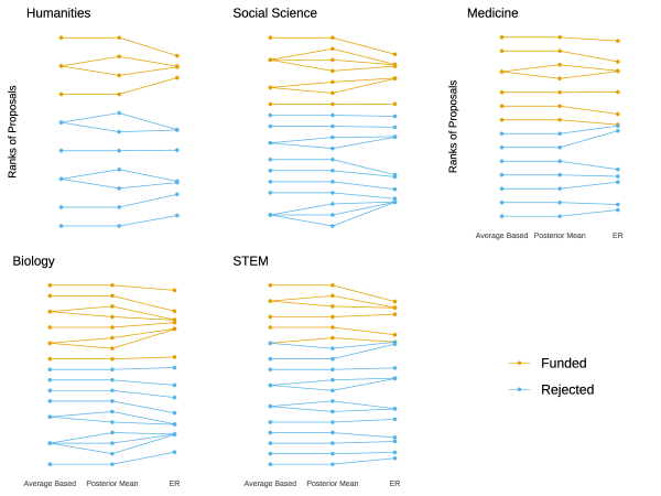
Figure 1: Junior fellowship proposals ranked based on simple averages (points on the left), the posterior means (middle) and the ER (points on the right), by the evaluation panel. Note that rank 1, displayed on the top, is the best rank. The color indicates the proposals funded if the best proposals based on the ER and constrained by the number of fundable proposals are funded.

Figure 2 plots the ERs of the same proposals together with their 50% credible intervals and the provisional funding line ($=$ the ER of the last fundable proposal). This presentation facilitates identifying proposals that cluster around the funding line; i.e. the proposals that might be included in a lottery (or random selection group). The methodology supports the following decisions:

• Humanities panel: The four best ranked proposals are funded, the remaining seven are rejected, no random selection.

• Social Sciences: The seven best ranked proposals are funded, the eleven worst ranked proposals are rejected, no random selection.

• Medicine: The five best ranked proposals are funded, the five worst ranked proposals are rejected. Two proposals are randomly selected for funding among the four proposals ranked as sixth to ninth.

• Biology: The eight best ranked proposals are funded, the ten worst ranked proposals are rejected, no random selection.

• STEM: The four best ranked proposals are funded, the ten worst ranked proposals are rejected. Two proposals are randomly selected for funding among the four proposals ranked as fifth to eighth.

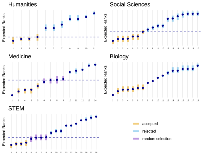
Figure 2: Bayesian Ranking: The expected rank as point estimates (posterior mean), together with 50% credible intervals (colored boxes). The dashed blue line is the provisional funding line, $i.e.$ the ER of the last fundable proposal. The color code indicates the final group the proposal is in: accepted or rejected proposals, or random selection/lottery group.

Samples from the posterior distributions of all the parameters in the Bayesian hierarchical model can be extracted from the JAGS model. This allows the funders to better understand the evaluation process. As a reminder, parameter $\nu_{j}$ summarises the behavior of panel member $j$. The more $\nu_{j}$ is negative, the stricter the scoring behavior of assessor $j$ compared to the remaining panel members. This also means that the stricter grades from assessor $j$ are corrected more, because they comply with their usual behavior. Figure 3 shows the posterior distributions of the $\nu_{j}$’s for the Social Sciences and Medicine panels. Note that we only present these two panels, because they are small enough to allow interpretation. The illustration of the remaining panels can be found in Figure 1.4 in the online supplement. In the Social Sciences, assessor 8 is a more critical panel member, whereas assessor 14 gives, on average, the highest scores. Also in the Medicine panel, the distributions for the different assessors are quite different. This illustrates how important it is to account for assessor effects.

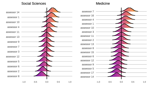
Figure 3: Posterior distributions of the assessor-specific means $\nu_{j}$ in the Social Sciences and Medicine panels. Each of the 14 assessors voted on up to 18 proposals, unless they had a conflict of interest or other reasons to be absent during the vote. Note that the 14 assessors in the Social Sciences panel were not the same as the ones in the Medicine panel.

Additionally, the posterior means of the variation of the proposal effects, $\tau_{\theta}^{2}$, for each panel with 90% CrI can be extracted: 0.14 with [0.06, 0.34] for the Humanities, 0.13 with [0.07, 0.25] for the Social Sciences, 0.18 with [0.1, 0.32] for the Biology Panel, 0.17 with [0.08, 0.34] for the Medicine panel and 0.17 with [0.09, 0.31] for the STEM panel. The same information can be retrieved for the variation of the assessor effect $\tau_{\lambda}^{2}$: 0.09 with [0, 0.25] for the Humanities, 0.07 with [0, 0.18] for the Social Sciences, 0.06 with [0, 0.16] for the Biology Panel, 0.07 with [0, 0.2] for the Medicine panel and 0.13 with [0, 0.34] for the STEM panel.

Further Figures, representing the rankograms and SUCRAs, the PCER and the ranking using the posterior mean of $\theta_{i}$ and their 50% CrI can be found in Figures 1.5 to 1.7 in the online supplementary material. For all the results of the panels presented above we used the convergence test described in Section 2.3.1 to ensure convergence of all chains.

Similar results are found when using the ordinal model defined in (2), see Figure 1.8 in the online supplementary material. Figure 1.9 in the online supplement shows the Bland-Altman plot [Bland and Altman, 1999] representing the agreement between the rankings based on the ordinal and continuous models, defined in equations (1) and (2) respectively.

3.2 Project Funding

Project Funding is the SNSF’s most important funding instrument. Project grants support blue-sky research of the applicant’s choice. We analyzed the proposals submitted to the April 2020 Call to the Mathematics, Natural and Engineering Sciences (MINT) division. Overall, the division evaluated 353 grant proposals. The evaluation was done in four sub-panels of the same size (nine members) and a similar number of international and female members. Each panel member evaluated all proposals (unless they had a conflict of interest), and each panel defined its own funding line aiming at a similar ($\sim 30\%$) success rate. Table 3 shows the total number of proposals, fundable proposals and average scores (from 1, poor, to 6, outstanding). Average scores were highest in panel 3 and lowest in panel 4.

Table 3: Summarising statistics in the four panels of the Mathematics, Natural and Engineering Sciences division in Project Funding.

Panel	N. of discussed proposals	N. of fundable proposals	Average score	Average score in top 30%
Panel one	87	26	3.84	5.01
Panel two	92	28	3.81	5.02
Panel three	86	26	3.97	5.24
Panel four	88	26	3.73	5.04

Table 4 shows the ICC (with 95% confidence interval). Figure 2.1 in the online supplement presents all the votes of the panel members in each sub-panel for each of the proposals. Compared to the previous Postdoc.Mobility case study, the intra-class correlation coefficients are higher and can be classified as good. One reason for the higher reliability here is that all Project Funding proposals are included - also the ones with low/high average scores, for which the votes are usually less variable. In contrast, for Postdoc.Mobility we only looked at the proposals with average scores in the middle range.

Table 4: The intra-class correlation coefficients together with their 95% confidence intervals of the different sub-panels. The overall reliability in the those panels can be classified as good.

	ICC (95% CI)
Panel one	0.82 (0.78; 0.86)
Panel two	0.85 (0.82; 0.89)
Panel three	0.85 (0.81; 0.88)
Panel four	0.82 (0.78; 0.86)

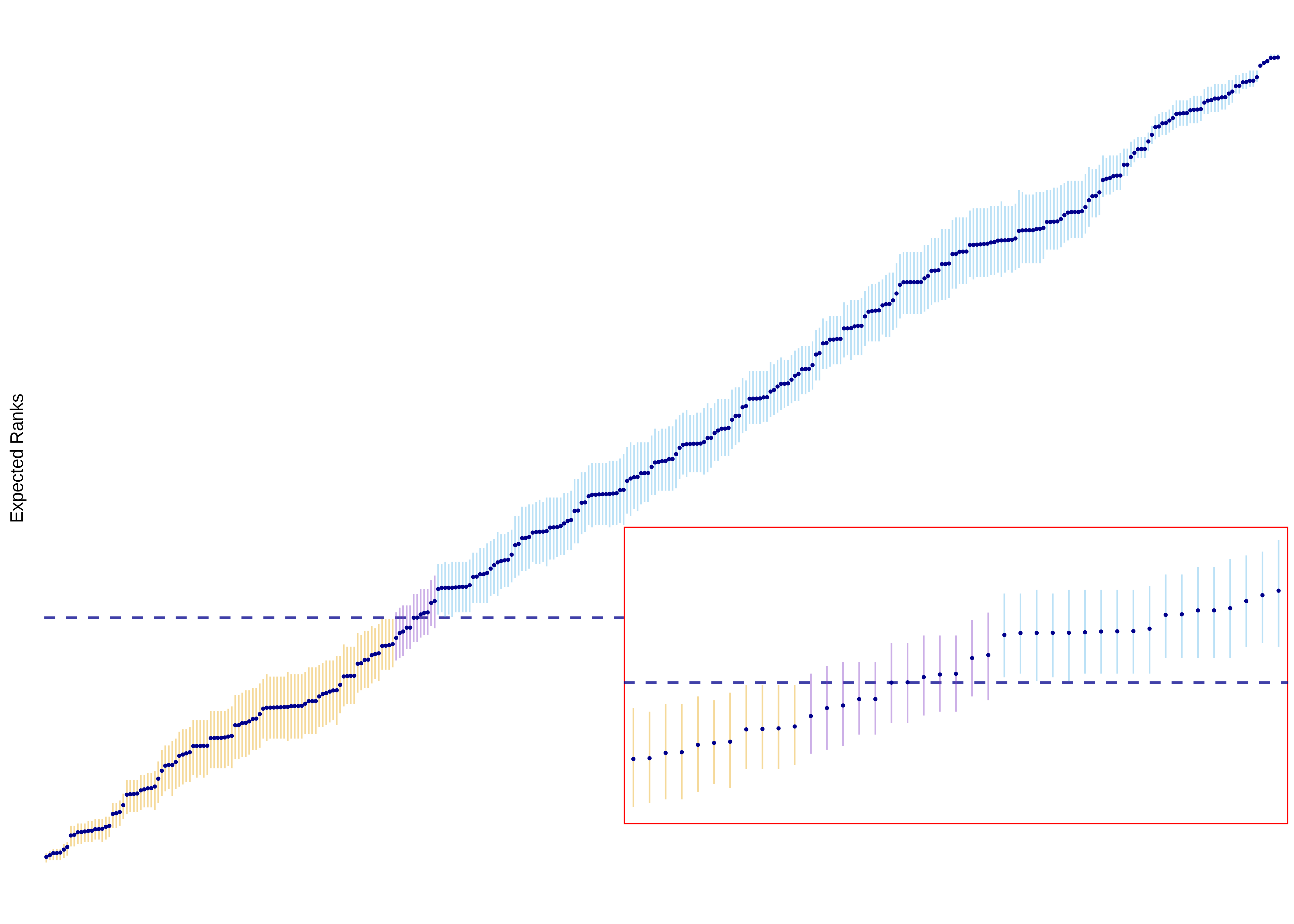
Figure 4: Bayesian Ranking: Proposals ordered from the best ER (bottom left, rank 1) to the worst (top right, rank 352) together with their 50% credible intervals. A provisional funding line to ensure a 30% success rate is drawn (blue dashed line). The proposals are arranged in three groups: funded (orange), random selection (violet) and rejected (blue).

In this case study, we illustrate the BR with an underlying model defined in (4), where an overall ranking is aimed for, while the evaluation was done in sub-panels. Figure 4 shows the ER ordered from the best-ranked proposal (bottom left) to the worst (top right) together with their 50% credible intervals. The provisional funding line is defined as the ER of the last fundable proposal: the 106th (30% of 353) best ranked, according to its ER. Zooming in on the provisional funding line shows the cluster of proposals with similar quality and 50% credible intervals overlapping with the funding line. These proposals may be included in the lottery/random selection group.

As for the Postdoc.Mobility evaluations, we can also estimate the variation of the proposal, assessor and panel effects (posterior mean with 90% CrI): 1.13 with [0.99, 1.28] for $\tau_{\theta}^{2}$, 0.09 with [0, 0.2] for $\tau_{\lambda}^{2}$ and 0.01 with [0, 0.12] for $\tau_{\delta}^{2}$. A more detailed analysis of this case study can be found in the online supplement (especially, also the results if using model (1) on the sub-panels seperately). For all the results presented above we again used the convergence test described in Section 2.3.1 to ensure convergence of all chains.

Similar results are found when using a Bayesian hierarchical model that explicitly accounts for the ordinal nature of the scores; see Figure 2.5 in the online supplement. Figure 2.6 in the online supplement shows the Bland-Altman plot; the agreement between the BR with an ordinal outcome model and the BR with a continuous outcome model. However, even though both models yield similar results, it is hard to say which modelling approach performs better without knowing exactly which proposals should have been funded or rejected. We therefore compare the performance of different models in a simulation study, where the true ranks are known.

4 Simulation Study

We conducted a simulation study to compare our proposed Bayesian ranking method (with continuous and ordinal outcomes, homogeneous and heterogeneous residuals) to the currently used procedure, i.e. the ranking based on averages. We closely follow Cao et al. [2010] to simulate the true ranks. We suppose that our panel is composed of $J=10$ members, who assess $I=50$ proposals on an ordinal scale from 1 to 6 (where 6 is the best score and 1 is the lowest). Note that in Cao et al.’s simulation study a five-point scale was used; to be as close as possible to our current scenario we use a six-point scale instead. The data is simulated from a model that is different from the one assumed for the computation of the Bayesian ranking. More specifically, we start with the ordinal outcome model in (2) and apply the following adaptations. For $j=1,\dots,10$, $\alpha_{j}\sim\mbox{Unif}(-0.5,0.5)$ and for $j=1,\dots,9$, the variation will be defined as $\sigma_{j}\sim\mbox{Unif}(0,0.5)$ and $\sigma_{10}=0.9$. We assume $\tau_{\theta}=1$, so that $\theta_{i}\sim N(0,1)$ for $i=1,\dots,I$. Finally, the latent variable $x_{ij}\sim N(\alpha_{j}+\theta_{i},\sigma_{j}^{2})$ and the final grade $y_{ij}$ is simulated with the cutoffs $c_{1}=-1,c_{2}=-0.5,c_{3}=0,c_{4}=0.5,c_{5}=1$. To mimic the possibility of conflicts of interest or abstentions in the data, we first draw a random number $M\in[1,100]$ for the number of missing scores and then randomly add $M$ missing values into the data matrix. We replicate these simulation steps $N=500$ times to achieve a small enough Monte-Carlo Error (see below). The code to simulate the data can be found in Appendix D. To estimate the Bayesian hierarchical models, we use 10’000 iterations, 5’000 burn-in and adaptation iterations and four chains.

The true ranks are computed using the simulated true proposal effects ($\theta^{\mbox{\tiny true}}_{i},i=1,\dots,J$): $R_{i}^{\mbox{\tiny true}}(\mathbf{\theta})=\mbox{rank}(\theta^{\mbox{\tiny true}}_{i})=\sum_{l=1}^{I}\mbox{I}(\theta^{\mbox{\tiny true}}_{i}>\theta^{\mbox{\tiny true}}_{l}).$ Then, in order to compare the different approaches to each other, and understand which method best estimated the true rank we will use the mean squared error (MSE) loss:

$$\mbox{MSE}=\frac{1}{I}\sum_{i}(R^{\mbox{\tiny true}}_{i}(\mathbf{\theta})-R_{i}^{est})^{2},$$

with $R_{i}^{est}$ being the estimated rank; the rank of proposal $i$ given by the procedure that is tested.

The approaches compared here are the ranking based on the average, the Bayesian Ranking (BR) with an underlying normal outcome model and homogeneous residuals (as described in (1)), the BR with an ordinal outcome model and homogeneous residuals (as described in (2)), the BR with a normal outcome model and heterogeneous residuals, and finally the BR with an underlying ordinal outcome model and heterogeneous residuals (both adapted from (3)). Table 5 compares the mean squared error of the different ranking approaches. Following the suggestion from Morris et al. [2019] we additionally calculated the Monte Carlo standard error (SE) for the MSE as follows

$$\mbox{Monte Carlo SE}=\frac{\sum_{i}\left((R^{\mbox{\tiny true}}_{i}(\mathbf{\theta})-R_{i}^{est})^{2}-\mbox{MSE}\right)^{2}}{N(N-1)}.$$

As mentioned in Cao et al. [2010] the MSE informs us on the ability of the procedure to accurately rank all the proposals. The best performing method is the BR with underlying ordinal model and heterogeneous residuals; the model closest to the data generating process. However, the simple BR with underlying normal outcome model and homogeneous residuals outperforms the remaining approaches. Hence, applying the Occam razor principle, favoring simpler models to complex models, we would suggest to use the BR approach as defined in model (1). The reason why this simpler model performs so well is most likely due to the fact that for the ordinal outcome model (and the heterogeneous residuals) an additional latent variable, the cutoffs and other parameters have to be estimated.

Table 5: Comparison of the MSE of the ranking estimators. SE stands for standard error.

	MSE	(Monte Carlo SE)
Rank based on average	4.310	(0.071)
BR: normal outcome with homogeneous residuals	3.715	(0.055)
BR: ordinal outcome with homogeneous residuals	3.807	(0.056)
BR: normal outcome with heterogeneous residuals	3.810	(0.056)
BR: ordinal outcome with heterogeneous residuals	3.517	(0.054)

5 Discussion

Inspired by work on ranking baseball players [Berger and Deely, 1988], health care facilities [Lingsma et al., 2010] and treatment effects [Salanti et al., 2011], we developed a Bayesian Ranking method based on a hierarchical model to support decision making on proposals submitted to the SNSF. A provisional funding line is defined based on the expected rank (ER) and the available budget. The ER and its credible interval are then used to identify proposals with similar quality and credible intervals that overlap with the provisional funding line. These proposals are entered into a lottery to select those to be funded. The approach acknowledges that there are proposals of similar quality and merit, which cannot all be funded. Previous studies suggested that peer review has difficulties in discriminating between applications that are neither clearly competitive nor clearly non competitive [Fang and Casadevall, 2016, Klaus and Alamo, 2018, Scheiner and Bouchie, 2013]. Decisions on these proposals typically lead to lengthy panel discussions, with an increased risk of biased decision making. The method proposed here avoids such discussions and thus may increase the efficiency of the process, reduce bias and costs.

The Bayesian ranking methodology compares every assessor to every other panel member. The ER considers all uncertainty in the evaluation process that can be observed and quantified. It accommodates the fact that different assessors have different grading habits. The model can also be adjusted for potential confounding variables, such as external peer reviewers’ characteristics that influence their scores. A recent analysis of 38’250 peer review reports on 12’294 SNSF project grant applications across all disciplines showed that male reviewers, and reviewers from outside Switzerland, awarded higher scores than female reviewers and Swiss reviewers [Severin et al., 2020]. Jayasinghe et al. [2003] modeled peer review records from the Australian Research Council using a multilevel cross-classified model in order to identify researcher and assessor attributes that influence the evaluation. They found low reliability in the scores attributed by the assessors, no gender effects, but an effect of the status of the University and the academic rank of the first applicant.

We agree with Goldstein and Spiegelhalter [1996] who argued that “no amount of fancy statistical footwork will overcome basic inadequacies in either the appropriateness or the integrity of the data collected”. In an ideal world, all proposals would be evaluated by as many experts it takes to ensure that meaningful differences between aggregated scores can be detected with confidence. Evaluations would be unbiased and describe nothing else but the quality of the proposals. Human nature and limited resources regarding time and funding sadly prevent this ideal situation from becoming a reality. The evaluation of grant proposals will always be subjective to some extent and affected by unconscious biases and chance. However, we are confident that the method presented here is an improvement over the commonly used approaches to ranking proposals and defining funding lines. Our approach should not be seen as a mechanistic cookbook approach to decision making but as a tool that can provide decision support for proposals of similar or indistinguishable quality around the funding line. For example, judgement continues to be required to decide whether a lottery should be used or not.

We applied the approach to two instruments in career and project funding at the SNSF. Our case studies addressed the specific context of the SNSF and the two funding schemes and results may not be generalizable to other instruments or funders. Further, we acknowledge that the team carrying out this study included several researchers affiliated with the SNSF. As the researchers’ expectations might influence interpretation, critical comment and review of our approach from independent scholars and other funders will be particularly welcome.
In our first model, we treated the ordinal scores (from 1 to 6) as continuous variables, thus assuming that the distance between each set of subsequent scores is equal. This assumption might not always be appropriate, but it builds on the currently used average-based ranking method, as this procedure also assumes normality of the grades. We showed how our initial model can be generalised to allow for an ordinal outcome variable. However, because of the fact that for the ordinal model extra parameters have to be estimated and in the simulation studies this more general model did not always perform better, we suggest to use the simpler model based on the normal likelihood.

The choice of priors in Bayesian models is always disputable. Especially for the variance parameters, alternative prior distributions could be investigated, like half-normal and half-Cauchy priors, whereas inverse-Gamma priors are generally not recommended [Gelman, 2006]. Instead of a Gibbs sampler, the brms-package in R [Bürkner, 2018] can be used, which makes the programming language Stan accessible with commonly used mixed model syntax, similar to the lme4-package by Bates et al. [2015]. Another approach is to use the R code provided by Lingsma et al. [2010]. They implemented a frequentist approach where the posterior means and variances of the proposal-specific random intercept are approximated. However, if the proposal effects are a posteriori dependent, because of the same assessors evaluating the same set of proposals, the Bayesian approach is easier to implement.

The use of a lottery to allocate research funding is controversial. At the SNSF the applicants are informed about the possible use of random selection, thus complying with the San Francisco Declaration on Research Assessment [DORA, 2019], which states that funders must be explicit about assessment criteria. Of note, in the context of the Explorer Grant scheme of the New Zealand Health Research Council, Liu et al. [2020] recently reported that most applicants agreed with random selection. So far, the SNSF received no negative or positive reactions to the use of random selection from applicants [Bieri et al., 2021]. The lottery element being controversial is also the reason why we start using the Bayesian ranking methodology with a 50% CrI. This ensures that the random selection groups are reasonably small.

An alternative to ranks based on simple averages of scores is the procedure employed by the National Institutes of Health (NIH). The NIH uses percentile rankings to define a funding line: proposals are first discussed and assigned scores from 1 to 9 by all panel members. For each proposal, all scores are then averaged to obtain an overall impact score. Finally, percentiles are determined by matching overall impact scores against historical relative rankings (based on the last three calls/review cycles). The NIH procedure makes a relative ranking possible by putting the different scores in context, however, when drawing the funding line (or payline), the uncertainty of the estimated quantities is not taken into account. This is an important difference to a ranking based on PCER (which is also percentile-based), ER or SUCRA. Ignoring uncertainty is especially problematic since there is evidence that the percentile scores employed by the NIH are poorly predictive of grant productivity [Fang et al., 2016].

In conclusion, we propose that a Bayesian modelling approach to ranking proposals combined with a modified lottery can improve the evaluation of grant and fellowship proposals. More research on the limitations inherent in peer review and grant evaluation is needed. Funders should be creative when investigating the merit of different evaluation strategies [Severin and Egger, 2020]. We encourage other funders to conduct studies and test evaluation approaches to improve the evidence base for rational and fair research funding.

Supplemental Materials and Data

An online fully reproducible supplement is provided which uses an R (ERforResearch) package with the implementation of the above presented methodology (see snsf-data.github.io/ERpaper-online-supplement/). The data used in the case studies can be downloaded from Zenodo: https://doi.org/10.5281/zenodo.4531160.

Appendix

A Analytical formulas

This section will give some insights on how the previously discussed quantities can be computed analytically rather than using MCMC samples. The probability of $\theta_{i}$ being smaller than $\theta_{k}$, which is used for the ER, can be computed as follows:

$$\mbox{Pr}(\theta_{i}\leq\theta_{k}) = \mbox{Pr}(\theta_{i}-\theta_{k}\leq 0)$$

$$= \mbox{Pr}\left(\frac{\theta_{i}-\theta_{k}-(\hat{\theta}_{i}-\hat{\theta}_{k})}{\sqrt{\mbox{var}(\hat{\theta}_{i})+\mbox{var}(\hat{\theta}_{k})-2\mbox{cov}(\hat{\theta}_{i},\hat{\theta}_{k})}}\leq\frac{-(\hat{\theta}_{i}-\hat{\theta}_{k})}{\sqrt{\mbox{var}(\hat{\theta}_{i})+\mbox{var}(\hat{\theta}_{k})-2\mbox{cov}(\hat{\theta}_{i},\hat{\theta}_{k})}}\right)$$

$$= \Phi\left(\frac{\hat{\theta}_{k}-\hat{\theta}_{i}}{\sqrt{\mbox{var}(\hat{\theta}_{i})+\mbox{var}(\hat{\theta}_{k})-2\mbox{cov}(\hat{\theta}_{i},\hat{\theta}_{k})}}\right),$$

where $\Phi$ is the standard normal cumulative distribution function. Here, $\hat{\theta}_{i}$ denotes the posterior expectation of $\theta_{i}$ and $\mbox{var}(\hat{\theta}_{i})$ and $\mbox{cov}(\hat{\theta}_{i},\hat{\theta}_{k})$ the corresponding posterior variance and covariance. If the $\theta_{i}$’s are a posteriori independent (which does in general not hold for model (1)), then $\mbox{cov}(\hat{\theta}_{i},\hat{\theta}_{k})=0$ for $i\neq k$.

There is also an analytical version of the posterior variance of the rank $R_{i}$ discussed in the Appendix of Laird and Louis [1989] that can be used to compute confidence intervals rather than credible intervals. According to the latter authors, this posterior variance is given by:

$$\mbox{var}(R_{i}) = \mbox{var}\left(\sum_{k=1}^{n}\mbox{I}(\theta_{i}\leq\theta_{k})\right)$$

$$= \sum_{k=1}^{n}\mbox{var}\left(\mbox{I}(\theta_{i}\leq\theta_{k})\right)+2\sum_{k=1}^{n}\sum_{l>k}\mbox{cov}\left(\mbox{I}(\theta_{i}\leq\theta_{k}),\mbox{I}(\theta_{i}\leq\theta_{l})\right)$$

$$= \sum_{k=1}^{n}\mbox{Pr}(\theta_{i}\leq\theta_{k})\cdot(1-\mbox{Pr}(\theta_{i}\leq\theta_{k}))+$$

$$\ \ \ \ \ 2\cdot\sum_{k=1}^{n}\sum_{l>k}\big{[}\mbox{Pr}(\theta_{i}\leq\mbox{min}(\theta_{k},\theta_{l}))-\mbox{Pr}(\theta_{i}\leq\theta_{k})\cdot\mbox{Pr}(\theta_{i}\leq\theta_{l})\big{]}.$$

B Relationship between ER and SUCRA

In the following, the relationship between the SUCRA and the ER is derived. Note that the ER, i.e. the expectation of the rank, can be expressed in terms of the rank probabilities as follows: $\mbox{ER}_{i}=\sum_{j=1}^{n}j\cdot\mbox{Pr}(i=j)$.

$$\mbox{SUCRA}_{i} = \frac{1}{n-1}\sum_{m=1}^{n-1}\mbox{cum}_{im}=\frac{1}{n-1}\sum_{m=1}^{n-1}\sum_{j=1}^{m}\mbox{Pr}(i=j)$$

$$(n-1)\mbox{SUCRA}_{i} = \sum_{m=1}^{n-1}\sum_{j=1}^{m}\mbox{Pr}(i=j)$$

$$(n-1)\mbox{SUCRA}_{i}-n = \sum_{m=1}^{n-1}\sum_{j=1}^{m}\mbox{Pr}(i=j)-\sum_{m=1}^{n}\sum_{j=1}^{n}\mbox{Pr}(i=j),\mbox{ because }\sum_{j=i}^{n}\mbox{Pr}(i=j)=1$$

$$-(n-1)\mbox{SUCRA}_{i}+n = -\sum_{m=1}^{n-1}\sum_{j=1}^{m}\mbox{Pr}(i=j)+\sum_{m=1}^{n}\sum_{j=1}^{n}\mbox{Pr}(i=j)$$

$$n-(n-1)\mbox{SUCRA}_{i} = \sum_{m=1}^{n-1}\sum_{j=m+1}^{n}\mbox{Pr}(i=j)+\sum_{j=1}^{n}\mbox{Pr}(i=j)$$

$$n-(n-1)\mbox{SUCRA}_{i} = \sum_{j=1}^{n}\mbox{Pr}(i=j)+\sum_{j=2}^{n}\mbox{Pr}(i=j)+\dots+\sum_{j=n}^{n}\mbox{Pr}(i=j)$$

$$n-(n-1)\mbox{SUCRA}_{i} = \sum_{j=1}^{n}j\cdot\mbox{Pr}(i=j)=\mbox{ER}_{i}$$

C Implementation of the Bayesian model in rjags and convergence diagnostics

The following code describes the definition of the model in R through the package rjags. Note that this JAGS model definition refers to the model described in (4), exactly as it is used in Section 3.2. Find more alternative model definitions in the function get_default_jags_model() in our package ERforResearch.

"model{

      # Likelihood:

      for (i in 1:n) { # i is not the application but the review

          grade[i] ~ dnorm(mu[i], inv_sigma2)

                # inv_sigma2 is precision (1 / variance)

          mu[i] <- overall_mean + application_intercept[num_application[i]] +

          voter_intercept[num_application[i], num_voter[i]] +

          section_intercept[num_section[i]]

      }

      # Ranks:

      rank_theta[1:n_application] <- rank(-application_intercept[])

      # Priors:

      for (j in 1:n_application){

        application_intercept[j] ~ dnorm(0, inv_tau_application2)

      }

      for (l in 1:n_voters){

        for(j in 1:n_application){

          voter_intercept[j, l] ~ dnorm(nu[l], inv_tau_voter2)

        }

      }

      for (l in 1:n_voters){

        nu[l] ~ dnorm(0, 4)

      }

      for (l in 1:n_section){

        section_intercept[l] ~ dnorm(0, inv_tau_section2)

      }

      sigma ~ dunif(0.000001, 2)

      inv_sigma2 <- pow(sigma, -2)

      inv_tau_application2 <- pow(tau_application, -2)

      tau_application ~ dunif(0.000001, 2)

      inv_tau_voter2 <- pow(tau_voter, -2)

      tau_voter ~ dunif(0.000001, 2)

      inv_tau_section2 <- pow(tau_section, -2)

      tau_section ~ dunif(0.000001, 2)

    }"

Trace plots and the $\widehat{R}$ values of the Gelman-Rubin convergence diagnostic of the most important parameters can be computed; see Figure 3.1 and Table 3.1 of the online supplement. For reproducibility purposes, the length of burn-in and adaptations phases, and the final number of iterations used in our case studies can be retrievd from our online supplement as well as the seed used for the sampling. With this information all models converged (with $\widehat{R}$ values lower to 1.1). Note that for convenience, we kept the numbers of iterations high and did not try to optimize. The online supplement also briefly discusses the sensitivity of the results to the choice of the hyperpriors; see Section 4 of the supplement.

D Code simulating data

Find the R code used for simulating the data in Section 4 below.

# Simulate data afer Cao et al.:

set.seed(0307)

J <- 10

j <- 1:J

I <- 50

N <- 500

sims <- list()

for (n in 1:N){

  alpha <- runif(J, -.5, .5)

  sigma <- runif(J - 1, 0, .5)

  sigma <- c(sigma, .9)

  c <- rep(NA, 5)

  c[1] <- -1

  c[2] <- -.5

  c[3] <- 0

  c[4] <- .5

  c[5] <- 1

  theta <- rnorm(I, 0, 1)

  x <- y <- matrix(NA, nrow = I, ncol = J)

  for (ii in 1:I){

    for (jj in 1:J){

      x[ii, jj] <- rnorm(1, alpha[jj] + theta[ii], sigma[jj]**2)

      y[ii, jj] <- 1

      if ((x[ii, jj] > c[1]) & (x[ii, jj] <= c[2])) y[ii, jj] <- 2

      if ((x[ii, jj] > c[2]) & (x[ii, jj] <= c[3])) y[ii, jj] <- 3

      if ((x[ii, jj] > c[3]) & (x[ii, jj] <= c[4])) y[ii, jj] <- 4

      if ((x[ii, jj] > c[4]) & (x[ii, jj] <= c[5])) y[ii, jj] <- 5

      if (x[ii, jj] > c[5]) y[ii, jj] <- 6

    }

  }

  # How many NAs/COIs do we want to introduce?

  n_nas <- sample(0:100, 1)

  # Which elements of the matrix will be NA?

  # Make sure, we did not set a whole column or row to NA

  test <- TRUE

  while (test){

    where_nas <- sample(1:(I*J), n_nas)

    xx <- x; yy <- y

    xx[where_nas] <- NA

    yy[where_nas] <- NA

    test <- any(rowSums(is.na(xx)) == J) | any(colSums(is.na(xx)) == I)

  }

  # Creation of data in list format

  sims[[n]] <- list(x = xx, y = yy, theta = theta, rank = rank(-theta))

}

References

- Adam [2019] David Adam. Science funders gamble on grant lotteries. Nature, 575(7784):574–575, November 2019. doi: 10.1038/d41586-019-03572-7.
- Alberts et al. [2014] Bruce Alberts, Marc W. Kirschner, Shirley Tilghman, and Harold Varmus. Rescuing US biomedical research from its systemic flaws. Proceedings of the National Academy of Sciences of the United States of America, 111(16):5773–5777, April 2014. doi: 10.1073/pnas.1404402111.
- Austrian Research Fund [2020] Austrian Research Fund. 1000 Ideas Programme, 2020. URL https://www.fwf.ac.at/en/research-funding/fwf-programmes/1000-ideas-programme.
- Bates et al. [2015] Douglas Bates, Martin Maechler, Benjamin M. Bolker, and Steven C. Walker. Fitting Linear Mixed-Effects Models Using lme4. Journal of Statistical Software, 67(1):1–48, October 2015. doi: 10.18637/jss.v067.i01.
- Berger and Deely [1988] Jo Berger and J. Deely. A Bayesian-Approach to Ranking and Selection of Related Means with Alternatives to Analysis-of-Variance Methodology. Journal of the American Statistical Association, 83(402):364–373, June 1988. doi: 10.2307/2288851.
- Bieri et al. [2021] Marco Bieri, Katharina Roser, Rachel Heyard, and Matthias Egger. Face-to-face panel meetings versus remote evaluation of fellowship applications: simulation study at the swiss national science foundation. BMJ Open, 11(5), 2021. doi: 10.1136/bmjopen-2020-047386.
- Bland and Altman [1999] J Martin Bland and Douglas G Altman. Measuring agreement in method comparison studies. Statistical Methods in Medical Research, 8(2):135–160, April 1999. doi: 10.1177/096228029900800204.
- Bromham et al. [2016] Lindell Bromham, Russell Dinnage, and Xia Hua. Interdisciplinary research has consistently lower funding success. Nature, 534(7609):684–687, June 2016. doi: 10.1038/nature18315.
- Bürkner [2018] Paul-Christian Bürkner. Advanced Bayesian Multilevel Modeling with the R Package brms. R Journal, 10(1):395–411, July 2018.
- Cao et al. [2010] Jing Cao, S. Lynne Stokes, and Song Zhang. A Bayesian approach to ranking and rater evaluation. Journal of Educational and Behavioral Statistics, 35(2):194–214, April 2010. doi: 10.3102/1076998609353116.
- Cicchetti [1993] Dv Cicchetti. The Reliability of Peer-Review for Manuscript and Grant Submissions - Its Like Deja-Vu All Over Again - Authors Response. Behavioral and Brain Sciences, 16(2):401–403, June 1993. doi: 10.1017/S0140525X0003079X.
- Cole et al. [1981] S. Cole, J. R. Cole, and G. A. Simon. Chance and consensus in peer review. Science (New York, N.Y.), 214(4523):881–886, November 1981. doi: 10.1126/science.7302566.
- DORA [2019] DORA. DORA – San Francisco Declaration on Research Assessment, 2019. URL https://sfdora.org/.
- Fang and Casadevall [2016] Ferric C. Fang and Arturo Casadevall. Research Funding: the Case for a Modified Lottery (vol 7, e00422, 2016). Mbio, 7(2):e00694–16, April 2016.
- Fang et al. [2016] Ferric C Fang, Anthony Bowen, and Arturo Casadevall. Nih peer review percentile scores are poorly predictive of grant productivity, 2016.
- Fogelholm et al. [2012] Mikael Fogelholm, Saara Leppinen, Anssi Auvinen, Jani Raitanen, Anu Nuutinen, and Kalervo Väänänen. Panel discussion does not improve reliability of peer review for medical research grant proposals. Journal of Clinical Epidemiology, 65(1):47–52, January 2012. doi: 10.1016/j.jclinepi.2011.05.001.
- Gelman [2006] Andrew Gelman. Prior distributions for variance parameters in hierarchical models (comment on article by Browne and Draper). Bayesian Analysis, 1(3):515–534, September 2006. doi: 10.1214/06-BA117A. Publisher: International Society for Bayesian Analysis.
- Gelman and Rubin [1992] Andrew Gelman and Donald B. Rubin. Inference from Iterative Simulation Using Multiple Sequences. Statistical Science, 7(4):457 – 472, 1992. doi: 10.1214/ss/1177011136.
- Gelman et al. [2014] Andrew Gelman, John B. Carlin, Hal S. Stern, David B. Dunson, Aki Vehtari, and Donald B. Rubin. Bayesian Data Analysis. Chapman and Hall/CRC, New York, NY, 3rd ed. edition, 2014. doi: 10.1201/b16018.
- Goldstein and Spiegelhalter [1996] Harvey Goldstein and David J. Spiegelhalter. League Tables and Their Limitations: Statistical Issues in Comparisons of Institutional Performance. Journal of the Royal Statistical Society. Series A (Statistics in Society), 159(3):385–443, 1996. doi: 10.2307/2983325. Publisher: [Wiley, Royal Statistical Society].
- Guthrie et al. [2018] Susan Guthrie, Ioana Ghiga, and Steven Wooding. What do we know about grant peer review in the health sciences? F1000Research, 6:1335, March 2018. doi: 10.12688/f1000research.11917.2.
- Guthrie et al. [2019] Susan Guthrie, Daniela Rodriguez Rincon, Gordon McInroy, Becky Ioppolo, and Salil Gunashekar. Measuring bias, burden and conservatism in research funding processes. F1000Research, 8:851, June 2019. doi: 10.12688/f1000research.19156.1.
- Harman [1998] Grant Harman. The Management of Quality Assurance: A Review of International Practice. Higher Education Quarterly, 52(4):345–364, 1998. doi: https://doi.org/10.1111/1468-2273.00104.
- Hedeker et al. [2008] Donald Hedeker, Robin J Mermelstein, and Hakan Demirtas. An application of a mixed-effects location scale model for analysis of ecological momentary assessment (EMA) data. Biometrics, 64(2):627–634, June 2008.
- Jayasinghe et al. [2003] Upali W. Jayasinghe, Herbert W. Marsh, and Nigel Bond. A multilevel cross-classified modelling approach to peer review of grant proposals: the effects of assessor and researcher attributes on assessor ratings. Journal of the Royal Statistical Society: Series A (Statistics in Society), 166(3):279–300, October 2003. doi: 10.1111/1467-985x.00278.
- Johnson [2008] Valen E Johnson. Statistical analysis of the national institutes of health peer review system. Proceedings of the National Academy of Sciences of the United States of America, 105(32):11076–11080, 2008.
- Kaatz et al. [2014] Anna Kaatz, Belinda Gutierrez, and Molly Carnes. Threats to objectivity in peer review: the case of gender. Trends in Pharmacological Sciences, 35(8):371–373, August 2014. doi: 10.1016/j.tips.2014.06.005.
- Kaplan et al. [2008] David Kaplan, Nicola Lacetera, and Celia Kaplan. Sample Size and Precision in NIH Peer Review. PLOS ONE, 3(7):e2761, July 2008. doi: 10.1371/journal.pone.0002761. Publisher: Public Library of Science.
- Klaus and Alamo [2018] Bernd Klaus and David del Alamo. Talent Identification at the limits of Peer Review: an analysis of the EMBO Postdoctoral Fellowships Selection Process. bioRxiv, page 481655, December 2018. doi: 10.1101/481655. Publisher: Cold Spring Harbor Laboratory Section: New Results.
- Laird and Louis [1989] Nan M. Laird and Thomas A. Louis. Empirical Bayes Ranking Methods. Journal of Educational Statistics, 14(1):29–46, 1989. doi: 10.2307/1164724. Publisher: [Sage Publications, Inc., American Educational Research Association, American Statistical Association].
- Lingsma et al. [2010] H.F. Lingsma, E.W. Steyerberg, M.J.C. Eijkemans, D.W.J. Dippel, W.J.M. Scholte Op Reimer, H.C. Van Houwelingen, and The Netherlands Stroke Survey Investigators. Comparing and ranking hospitals based on outcome: results from The Netherlands Stroke Survey. QJM: An International Journal of Medicine, 103(2):99–108, February 2010. doi: 10.1093/qjmed/hcp169.
- Liu et al. [2020] Mengyao Liu, Vernon Choy, Philip Clarke, Adrian Barnett, Tony Blakely, and Lucy Pomeroy. The acceptability of using a lottery to allocate research funding: a survey of applicants. Research Integrity and Peer Review, 5(1):3, February 2020. doi: 10.1186/s41073-019-0089-z.
- Lucy et al. [2017] Liaw Lucy, Freedman Jane E., Becker Lance B., Mehta Nehal N., and Liscum Laura. Peer Review Practices for Evaluating Biomedical Research Grants: A Scientific Statement From the American Heart Association. Circulation Research, 121(4):e9–e19, August 2017. doi: 10.1161/RES.0000000000000158. Publisher: American Heart Association.
- Mayo et al. [2006] Nancy E. Mayo, James Brophy, Mark S. Goldberg, Marina B. Klein, Sydney Miller, Robert W. Platt, and Judith Ritchie. Peering at peer review revealed high degree of chance associated with funding of grant applications. Journal of Clinical Epidemiology, 59(8):842–848, August 2006. doi: 10.1016/j.jclinepi.2005.12.007.
- Morris et al. [2019] Tim P. Morris, Ian R. White, and Michael J. Crowther. Using simulation studies to evaluate statistical methods. Statistics in Medicine, 38(11):2074–2102, January 2019. doi: 10.1002/sim.8086. URL https://doi.org/10.1002/sim.8086.
- Plummer [2019] Martyn Plummer. Package ‘rjags’. Bayesian Graphical Models using MCMC, November 2019.
- Salanti et al. [2011] Georgia Salanti, A. E. Ades, and John P. A. Ioannidis. Graphical methods and numerical summaries for presenting results from multiple-treatment meta-analysis: an overview and tutorial. Journal of Clinical Epidemiology, 64(2):163–171, February 2011. doi: 10.1016/j.jclinepi.2010.03.016.
- Scheiner and Bouchie [2013] Samuel M. Scheiner and Lynette M. Bouchie. The predictive power of NSF reviewers and panels. Frontiers in Ecology and the Environment, 11(8):406–407, 2013. doi: https://doi.org/10.1890/13.WB.017.
- Severin and Egger [2020] Anna Severin and Matthias Egger. Research on research funding: an imperative for science and society. British Journal of Sports Medicine, pages bjsports–2020–103340, November 2020. doi: 10.1136/bjsports-2020-103340.
- Severin et al. [2020] Anna Severin, Joao Martins, Rachel Heyard, Francois Delavy, Anne Jorstad, and Matthias Egger. Gender and other potential biases in peer review: cross-sectional analysis of 38 250 external peer review reports. Bmj Open, 10(8):e035058, 2020. doi: 10.1136/bmjopen-2019-035058.
- Shrout and Fleiss [1979] Patrick E. Shrout and Joseph L. Fleiss. Intraclass correlations: Uses in assessing rater reliability. Psychological Bulletin, 86(2):420–428, 1979. doi: 10.1037/0033-2909.86.2.420.
- van der Lee and Ellemers [2015] Romy van der Lee and Naomi Ellemers. Gender contributes to personal research funding success in The Netherlands. Proceedings of the National Academy of Sciences of the United States of America, 112(40):12349–12353, October 2015. doi: 10.1073/pnas.1510159112.
- van Houwelingen et al. [2009] Hans C. van Houwelingen, Ronald Brand, and Thomas A. Louis. Empirical Bayes methods for monitoring health care quality. arXiv:2009.03058 [stat], September 2009. arXiv: 2009.03058.
- Volkswagen Foundation [2017] Volkswagen Foundation. Experiment! – In search of bold research ideas, 2017. URL https://www.volkswagenstiftung.de/en/funding/our-funding-portfolio-at-a-glance/experiment.