A bi-level encoding scheme for the clustered shortest-path tree problem in multifactorial optimization

Abstract

The Clustered Shortest-Path Tree Problem (CluSPT) plays an important role in various types of optimization problems in real-life. Recently, some Multifactorial Evolutionary Algorithms (MFEAs) have been introduced to deal with the CluSPT, but these researches still have some shortcomings, such as evolution operators only perform on complete graphs and huge resource consumption for finding the solution on large search spaces. To overcome these limitations, this paper describes an MFEA-based approach to solve the CluSPT. The proposed algorithm utilizes Dijkstra’s algorithm to construct the spanning trees in clusters while using evolutionary operators for building the spanning tree connecting clusters. This approach takes advantage of both exact and approximate algorithms, so it enables the algorithm to function efficiently on complete and sparse graphs alike. Furthermore, evolutionary operators such as individual encoding and decoding methods are also designed with great consideration regarding performance and memory usage. We have included proof of the repairing method’s efficacy in ensuring all solutions are valid. We have conducted tests on various types of Euclidean instances to assess the effectiveness of the proposed algorithm and methods. Experiment results point out the effectiveness of the proposed algorithm existing heuristic algorithms in most of the test cases. The impact of the proposed MFEA was analyzed, and a possible influential factor that may be useful for further study was also pointed out.

1 Introduction

In the years following massive globalization efforts, clustered problems have found great interest, not only within the confinement of research communities but even more so from members of governments, international enterprises, or streaming services. This need for an ordered structure in a world that grows increasingly closer in proximity comes about as a natural consequence, and so too arises the need to solve a problem whose ever-present trace can be found in this internationalized age. Evidently, there are more obvious examples of goods delivery within metropolitan areas and large-scale shipments between countries. There is also the problem of schedule planning for public transportation, optimization of the distribution network for streaming services, the arrangement of stores within shopping malls, and on the more abstract, conceptual side, structuring human resources of a project. One of the better known clustered tree problems is a variant of the shortest path tree problem, named Clustered Shortest-Path Tree Problem (CluSPT) [1]. Being NP-Hard, the preferred method to tackle this problem has mainly by means of approximation algorithms, as solving a large instance of the CluSPT using exact approaches is unfeasible and quite literally a waste of time.

A family of global optimization algorithms that has found considerable success in dealing with NP-Hard problems are Evolutionary Algorithms (EAs) [2, 3]. These algorithms based their mechanisms on Darwin’s theory of evolution and natural selection. Essentially, a multitude of solutions will first be randomized, encoded in a way that the solutions are susceptible to changes by evolution operators, namely mutation and crossover, which will be further elaborated later on in this paper. The quality of solutions, henceforth be called as individuals, should increase upon subsequent generation. While EAs themselves have been subjects of research since the 1990s or, if one were to consider their more remote conception, the 1970s, this paper is based on a recent variation of the algorithm, the Multifactorial Evolutionary Algorithm (MFEA) [4, 5]. The MFEA operates on the same principle as the EA, but with a few adjustments to let it solve multiple problems at once as opposed to the EA. This fundamental change differs the MFEA greatly from its ancestor, using the fitness landscapes of multiple problems to help complement each problem’s solution, a concept known as cultural transmission, whereas the EA has to navigate this fitness landscape alone and thus more prone to stuck in local optimal. The MFEA has found great success in solving different types of problems due to this implicit genetic transfer between tasks in a multitasking environment [6, 7, 8].

Accordingly, the MFEA has been used in many research dealing with the CluSPT [9, 10, 11, 12], applying different evolutionary operators and mechanisms to the base algorithm. However, because the MFEA solves multiple problems concurrently, each one with their own restrictions and distinct search space, many of these researches could not confidently satisfy all these restrictions, even if all the problems the MFEA has to solve is the same type with different inputs. As a result, the final solution sometimes turns out to be an invalid one, incompatible with the original search space. This paper introduces an approach that is capable of remedying this fatal drawback. Furthermore, as this approach combines both the approximation aspect of the MFEA and the exact aspect of Dijkstra’s algorithm [13], it also improves the ultimate solutions, when compared to past algorithms on the CluSPT. Finally, we test the algorithm’s effectiveness when using multiple parents in the crossover process instead of the default two.

The major contributions of this work are as follows:

• Develop a new solution representation for the CluSPT, thus reducing resource consumption. This enhancement becomes especially more noticeable for instances of large proportion, whose population grows exponentially with size to ensure randomness and diversity.

• Devise a novel two-level scheme to solve the nested structure of the CluSPT: tree containing sub-trees. This scheme divides the CluSPT into an approximation problem and an exact problem, resulting in better solutions compared to pure approximation approaches while reducing the computational time as opposed to exact approaches.

• Propose a method to repair invalid individuals, ensuring that proposed evolutionary operators always produce a valid solution. The maximum number of fixes on an individual is also provided and proven.

• Design a crossover operator that can work with multiple parents.

• Propose an effective memory-based method to calculate the cost of CluSPT solution to increase the algorithm’s performance.

• Analyze the experimental results on a diverse range of test instances, with additional comparison to other algorithms, to demonstrate this proposed algorithm’s efficacy.

The rest of this paper is organized as follows. Section 2 presents the notations and definitions used for formulating problem. Section 3 introduced related works. The proposed MFEA for the CluSPT is elaborated in Section 4. Section 5 explains the setup of our experiments and analyzes the computed results. The paper concludes in Section 6 with discussions on the future extension of this research.

2 Problem definition and notations

The CluSPT is defined on a simple, connected and undirected graph $G(V,E,C,w,s)$ with a set of vertices $V$, a set of edges $E$, a set of clusters $C$, a weight matrix $w$, and a source vertex $s$, respectively. Set of vertices V is divided into $m$ clusters $C^{j},j=1...m$, $V=C^{1}\cup C^{2}\cup...\cup C^{m}$ and set of clusters $C=\{C^{1},C^{2},...,C^{m}\}$. A solution to this problem is a spanning tree $T$ whose sum of routing cost from the source vertex $s$ to all vertices in $V$ is minimum and the subgraph induced by all vertices in each cluster is also a spanning tree.

Given a spanning tree $T$ of $G$, let $d_{T}(u,v)$ denotes the shortest path length between $u$ and $v$ on $T$. The CluSPT is defined as following:

Clustered Shortest-Path Tree Problem
Input:	- A weighted undirected graph $G=(V,E,w)$.
	- Vertex set $V$ is partitioned into $k$ clusters ${V_{1},V_{2},...,V_{k}}$.
	- A source vertex $s$.
Output:	- A spanning tree $T$ of $G$
	- Sub-graph $T[V_{i}](i=1,\ldots,k)$ is a connected graph.
Objective:	$\displaystyle\sum_{v\in V}d_{T}(s,v)\rightarrow$ min
	where $d_{T}(u,v)$ is the cost of shortest path from vertex $u$ to vertex $v$ on $T$.

Definition 2.1.

For each cluster $C^{j}$ in $G$, $C^{j*}$ denotes the set of vertices connecting directly to vertices in other clusters. We call it the inter-vertices set of that cluster. An example is shown in Figure 2. Figure 1(a) presents an initial input graph $G$ has 14 vertices and 3 clusters. Figure 1(b) presents the set of inter-vertices of the corresponding cluster in $G$.

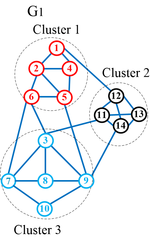
(a)

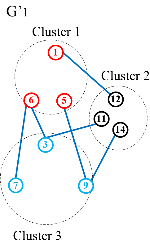
(b)

Figure 1: Sets of inter-vertices of the corresponding clusters in graph

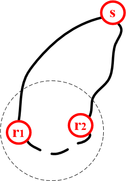
Figure 2: A spanning tree if exits a cluster having two local roots

Definition 2.2.

In the spanning tree $T$ obtained from the CluSPT problem, we denote a cluster’s level by its proximity to the root cluster. The level of the cluster that contains the source vertex s is 0, the cluster directly connected to it is level 1, the cluster directly connected to a level 1 cluster is level 2,…etc. It is obvious that each non-root cluster has a single vertex serving as the entrance from a lower level cluster. We call this the local root of the cluster.

Lemma 2.1.

Each cluster in the spanning tree T has only one local root.

Proof.

Assume that a cluster has more than one local root. Without loss of generality, we consider two local roots $r_{1}$ and $r_{2}$ of this cluster. There must exist a path $p_{s,r_{1}}$ from the source vertex $s$ of $T$ to $r_{1}$ without going through $r_{2}$ and a path $p_{s,r_{2}}$ from source vertex $s$ of $T$ to $r_{2}$ without going through $r_{1}$. In addition, the vertices $r_{1}$, $r_{2}$ belonging to the same cluster, so they will connect with each other, i.e there exists a path $p_{r_{1},r_{2}}$ from $r_{1}$ to $r_{2}$. As a result, a cycle exists on $T$ illustrated in Figure 2. This contradicts the requirement of $T$ being a spanning tree. The assumption is thus proven wrong. Therefore, each cluster in $T$ has only one local root meaning that every path from source vertex $s$ to vertices in a cluster in $T$ must go through its local root. Also, starting from $s$, a local root must be the first vertex to be visited within its own cluster. Because a local root is connected to a cluster of the lower level, the vertices selected as the local root of a cluster are in the cluster’s inter-vertices set. It is for this reason that we have deemed only the inter-vertices necessary for being encoded.

∎

3 Related works

Researches on cluster problems could be traced back to the 1970s [14]. One of the earliest related studies is the Clustered Traveling Salesman Problem [15, 16], whose objective is to determine the Hamiltonian path with a minimum length such that all vertices in each cluster are visited consecutively. As a cluster problem, the CluSPT [1] has just recently been explored but has already attracted much interest from the research community. Because CluSPT is NP-Hard, exact algorithms for such problems require exponential execution time and are only suitable for small instances. Therefore the approximation approaches are more suitable to deal with the CluSPT.

In recent literature, MFEA [17] has been emerging as an effective framework to solve a wide range of optimization problems. MFEA surpasses traditional EA [18] in its ability to simultaneously solve multiple problems, especially for systems with limited computational resources. Some preliminary works have been carried out, suggesting that MFEA is able to utilize the knowledge exchanging across relevant tasks to facilitate finding optimal solutions for multiple problems at the same time [19].

Consider Parting Ways [20], the authors proposed a new mechanism to reallocate resources within the process of MFEA. This mechanism has stemmed from the observation that while exchanging genetic material across tasks is beneficial to the evolutionary algorithm’s performance, but it can at times weaken exploitation and consume needless resources. More specifically, it is noted that the offspring generated from parents with different skill factors (called divergents) may help with the preservation of diversity within the population and allow information sharing to occur between tasks. However, as the population begins converging toward the optima of tasks, such contributions are irrelevant and, in cases, become obstacles for the convergence process. Therefore, a new measure ASRD, or Accumulated Survival Rate of divergents, was proposed to detect the point where information sharing is no longer desirable. In each generation, a ratio of divergents is created and survives to the next generation. The ASRD is the total of this ratio observed in a sliding window manner over several generations. Once ASRD is lower than a parameter value, the algorithm is set to never produce any divergent for the remaining duration.

According to Group-based [21], the authors aimed to improve the MFEA by mean of a clustering-based approach. It was discovered that in MFEA, the closer the global optima of two tasks are, or in general, the more similar the landscapes of two tasks are, the more likely it is for information sharing to have a positive impact. A new mechanism is built upon this discovery to maximize the advantage of information sharing in MFEA. More specifically, while the landscapes of tasks are mostly unknown, they can be roughly estimated by the distribution of the fittest individuals for each task. The new MFEA picks a representative for each task before comparing them using Manhattan distance, effectively clustering these representatives based on their likeness in genetic structure. Some representatives are further tested by exploring other clusters with regard to their skill factors. Should any cluster proved fruitful for the representatives, and more broadly for the task at which the representative is best at, improvement, then the representatives will be reassigned to such groups. Within one group, mating is only permitted if it could create better offspring. In addition, the authors also proposed a selection criterion to balance fitness value and diversity both in the mating and environmental selection (choosing individuals for the next generation) stage. This criterion is determined by the individual normalized fitness value and its crowding distance from its neighbors, together monitored by a balancing factor $\alpha$.

In Dynamic Resource Allocation [6], the authors designed a way of dynamically reallocating resources for each task in MFEA and a method to control information sharing inside a particular task and across tasks. It is a fact that in solving multiple tasks, rarely comes the case where each task is of approximately equal hardness. Thus, it appears counter-intuitive to distribute computational resources equally among the tasks. The new mechanism split the population into subpopulation, each specializing in one task. A subpopulation consists of a specific number of fittest individuals for that task along with some random individuals, the number of whom monitored by a learning parameter that updates itself every iteration, whose participation serves to introduce cross-domain genetic information. All subpopulations then run through several generations to record the improvement of population $\omega_{k}$. This measurement is the ratio of change between a task’s best fitness value of this generation and the one some generation before. The greater the ratio, that is, the more the best fitness value improves, the better the chance of a task being selected for resource allocation, denoted by Index of Improvement, or IoI. The IoI of a task is its improvement of the population over the total of all improvement of population. Thus, an IoI exists in the range of [0,1], and the selecting process is a Roulette one.

Yuan Yuan et al. [22] investigated the use of MFEA, specifically on Permutation-based Combinatorial Optimization Problems. The authors noted that the use of random key encoding for chromosomes proved ineffective for this kind of problem and suggested another unified representation scheme and a new survivor selection method. Since the chromosome for each task is always a permutation sequence, the new representation has the unified chromosome be a sequence of the task with the highest dimension. For each task, it simply removes genes with values greater than the task’s dimension while keeping the remaining genes in the same order. The introduced survivor selection method, dubbed as Level-based Selection, or LBS, sort the population into $K$ lists corresponding to $K$ optimization tasks. After the mating stage and all offspring have been put into the lists with regard to their skill factor, the list is sorted in ascending order (assuming, without loss of generality, that the tasks are minimization tasks), and an individual position in its list denotes its level. The population of the next generation is chosen from across all lists, and an individual can never be chosen if there is still another individual with a lower level in one of the lists.

Improvements upon the original MFEA have been met with considerable success. MFEA-II [19], from the same authors, tackled the centralizing idea of the algorithm itself: the knowledge transfer between tasks. While individuals excelling in the same task can reproduce freely, on the intra-task crossover, MFEA allows only a fixed percentage of the population (this percentage denoted by random mating probability, or $rmp$). This paper thus described in detail a probability-based system to measure the effectiveness of this knowledge transfer. In essence, as each task still exists individually, that is, separated into their own solution spaces (and by mean of MFEA can they find a common representation), the intra-task learning process may prove itself an obstacle for reaching optimal solutions. This is where MFEA-II comes into play, an algorithm that can adapt and change accordingly the $rmp$ and, if need be, cut off knowledge transfer altogether. If previous MFEA algorithms have depended on a fixed $rmp$ (commonly 0.5), MFEA-II formulates $rmp$ as a $n\times n$ matrix, assuming the number of tasks is $n$. This matrix reflects the relationship between tasks, with $rmp_{a,b}$ denotes how well $task_{a}$ and $task_{b}$ influence each other. Naturally, the matrix is symmetrical, as the relation between $task_{a}$ and $task_{b}$ is the same as $task_{b}$ and $task_{a}$. As each task corresponds perfectly to itself, the main diagonal line is all 1. This $rmp$ matrix changes itself upon each iteration, each generation, eventually erasing bad relationships while promoting good ones. The MFEA-II has found great success on many different implementations, surpassing state-of-the-art strategies like separable natural evolutionary strategy or exponential natural evolutionary strategy.

In recent years, some approximation approaches were developed for solving CluSPT. In [9], the authors proposed MFEA (hereinafter E-MFEA) with new genetic operator algorithm. The major idea of this novel genetic operators is that first comes the construction of a spanning tree for the smallest sub-graph, afterward spanning trees for larger sub-graphs are created from the spanning tree of smaller sub-graphs. In [10], the authors took advantage of the Cayley code to encode the solution of CluSPT and proposed genetic operators. The genetic operators introduced here are, conceptually, similar to the genetic operator for binary and permutation representations. However, it limits its application to complete graphs only. Therefore, the novel MFEA, too, is suitable exclusively for complete graphs. Binh at.el. [23] discussed a new algorithm based on the EA and Dijkstra’s Algorithm. In a divide and conquer fashion, the proposed algorithm decomposes the CluSPT problem into two sub-problems. The first sub-problem’s solution is found by an EA, while Dijkstra’s Algorithm solves the second sub-problem. The goal of the first sub-problem is to determine a spanning tree that connects among the clusters, while that of the second sub-problem is to determine the best-spanning tree for each cluster. In [12], the authors described a method of applying MFEA based on deconstructing an original problem into two problems. In the proposed MFEA, the second task plays a role as a local search method for improving the solutions that are determined in the first task.

Although some MFEA algorithms were proposed for solving CluSPT problem in practice, they have revealed multiple drawbacks, i.e., only applicable on complete graphs, inefficient for finding the solution on large search spaces, each task only finds the solution of a different problem (differences in problem formulation or dimensionality) or the proposed evolution operators are only suitable for the CluSPT problem. Therefore, to overcome these drawbacks, a new MFEA based approach is henceforth introduced to solve CluSPT problems.

4 Proposed Algorithm

In this section, we introduce an approach based on MFEA with new encoding, decoding, and repairing schemes as well as new evolutionary operators to solve multiple CluSPT problems simultaneously. Each problem is interpreted as a single task in the multitasking environment. The $i^{th}$ CluSPT task is performed on a input graph $G_{i}=(V_{i},E_{i},w_{i},s_{i}),i=1,\ldots,K$ where $V_{i},E_{i},w_{i},s_{i}$ are set of vertices, set of edges, weight matrix and source vertex, respectively. $V_{i}$ is divided into $m_{i}$ clusters. The $j^{th}$ cluster of the $i^{th}$ task is denoted by $C_{i}^{j},j=1,\ldots,m_{i}$ and $C_{i}=\{C_{i}^{1},C_{i}^{2},\ldots,C_{i}^{m_{i}}\}$. The local root of the $j^{th}$ cluster of the $i^{th}$ task is denoted by $r_{i}^{j}$. The proposed algorithm’s structure is presented in Algorithm 1, and the implementation steps of the algorithm are discussed in detail in the following subsections.

1begin

2       $t\leftarrow 0$;

       /* Initialize initial population */

3       $P(0)\leftarrow$ Randomly generate $N$ individuals from USS $\triangleright$ Refer to Algorithm 2;

4       foreach individual $p_{i}\in P(0)$ do

5             Assign skill factor $\tau_{i}=i\%N+1$;

6             Construct the private representation $sr_{i}$ of individual $p_{i}$ in task $\tau_{i}$ $\triangleright$ Refer to Algorithm 3;

7             if $p_{i}$ doesn’t have a valid representation then

8                   Perform the Repairing Individual Method on $sr_{i}$ $\triangleright$ Refer to Algorithm 4;

9                  

10             Construct a two-level solution of the CluSPT $p^{\prime}_{i}$ based on $sr_{i}$ $\triangleright$ Refer to Algorithm 5;

11             Evaluate $p_{i}$ based on the CluSPT solution $p^{\prime}_{i}$ for task $\tau_{i}$ only;

12            

13       end foreach

14      Update scalar fitness of each individual in $P(0)$;

15      

16      while stopping conditions are not satisfied do

17            

18            Offspring population $P_{c}(t)\leftarrow\emptyset$;

19             while $|P_{c}(t)|<N$ do

20                   Choose $k$ individuals $p_{i}(i=1,\ldots,k)$ randomly from $P(t)$;

                   /* Perform crossover operator */

21                   if (All selected individuals have same a skill factor) or ($rand<rmp$) then

22                         $o_{i}(i=1,\ldots,k)\leftarrow$ Perform the multi-parent crossover on $p_{i}(i=1,\ldots,k)$ $\triangleright$ Refer to Algorithm 6;

23                        

24                        The skill factor of $o_{i}\leftarrow$ Select randomly the skill factor of the parent;

25                        

26                  else

                         /* Perform mutation operator */

27                         $o_{i}\leftarrow$ Perform mutation on each individual $p_{i}(i=1,\ldots,k)$ $\triangleright$ Refer to Algorithm 7;

28                         The skill factor of $o_{i}\leftarrow$ the skill factor of the individual $p_{i}(i=1,\ldots,k)$;

29                        

30                   end if

31                  

                  /* Construct the CluSPT solution and evaluate the offspring */

32                   Decode the private representation $sr_{i}$ of each individual $o_{i}$ $\triangleright$ Refer to Algorithm 3;

33                  

34                  if $sr_{i}$ is invalid then

35                         Repair $sr_{i}$ $\triangleright$ Refer to Algorithm 4;

36                        

37                   Construct the CluSPT solution based on the $sr_{i}$ $\triangleright$ Refer to Algorithm 5;

38                  

39                  Evaluate $o_{i}$ for task corresponding to assigned skill factor only;

40                   $P_{c}(t)\leftarrow P_{c}(t)\cup\{o_{i}\}$, $i=1,\ldots,k$;

41                  

42             end while

43            

44            $P_{B}(t)\leftarrow$ the top 50% best individuals from $P(t)$;

45             $R(t)\leftarrow P_{c}(t)\cup P_{B}(t)$;

46             Update scalar fitness of each individual in $R(t)$;

47             $P(t+1)\leftarrow$ Get $N$ fittest individuals from $R(t)$;

48             $t\leftarrow t+1$;

49            

50       end while

51      

52 end

53

Algorithm 1 Proposed Algorithm to solve multiple the CluSPT problems

4.1 Individual representation in the unified search space

The traditional EA process has typically been focused on efficiently solving a single optimization problem at a time. Each solution for a problem has a private representation separately. In MFEA, the representations of solutions in particular problems are combined into the unified representation to reduce computational time and take advantage of the transfer of knowledge among tasks when solving them simultaneously.

The Unified Search Space (USS) for $K$ tasks of the CluSPT is a graph $G_{u}(V,C,m)$ where:

• The set of vertices $V$ of $G_{u}$ is partitioned into $m$ clusters where $m=\max(m_{1},m_{2},\ldots,m_{K})$ and $m_{i}$, $i=1,\ldots,K$ is the number of clusters of the $i^{th}$ task.

• The $j^{th}$ cluster of $G_{u}$ is denoted by $C^{j}$, and $C^{j}$ = $C_{1}^{j*}\cup C_{2}^{j*}\cup\ldots\cup C_{K}^{j*}$ where $C_{i}^{j*}$ is the set of inter-vertices of the $j^{th}$ cluster in the $i^{th}$ task.

• The set of clusters $C=\{C^{1},C^{2},\ldots,C^{m}\}$.

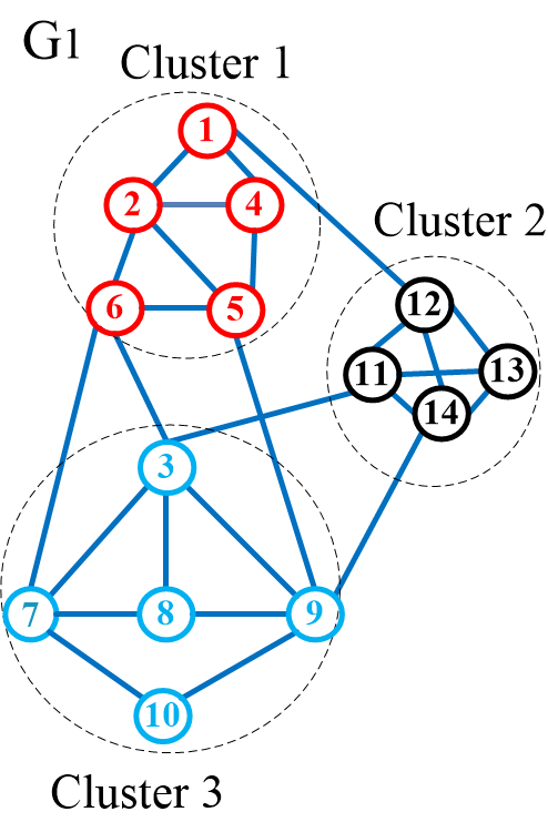
(a)

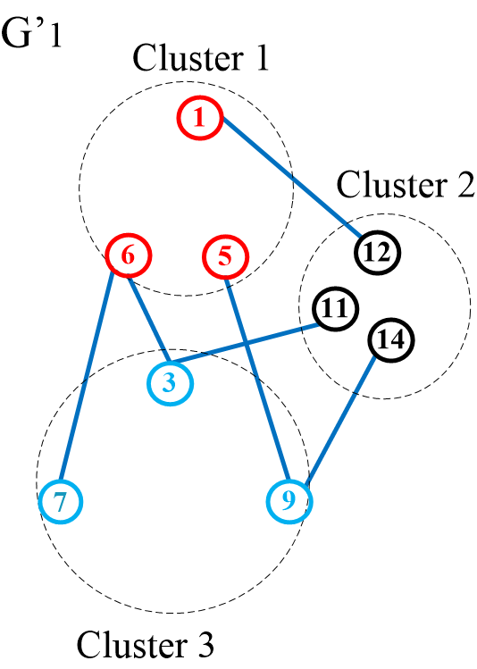
(b)

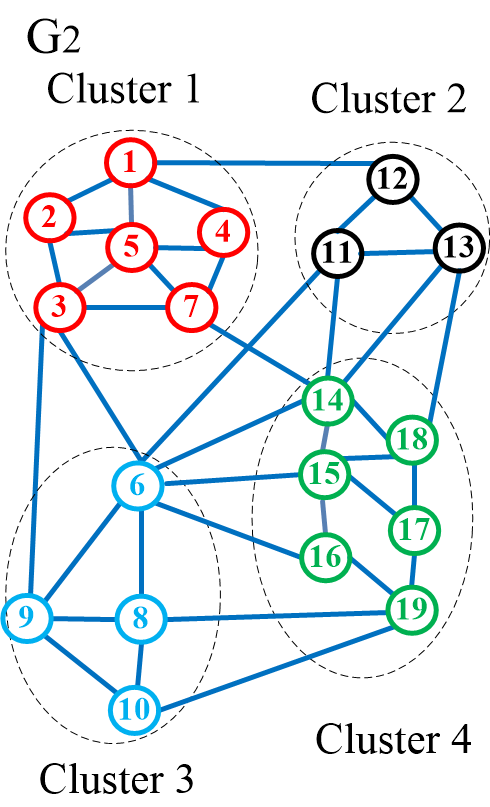
(c)

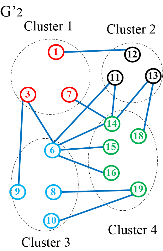
(d)

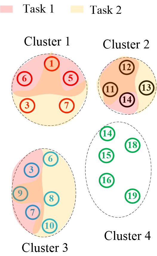
(e)

Figure 3: An example of a graph of the USS for MFEA with two tasks

Figure 3 illustrates steps to construct a graph $G_{u}(V,C,m)$ of the USS from the graphs of two tasks $T_{1}$ and $T_{2}$. Figure 3(a) and Figure 3(c) describe the input graphs of the two tasks where graph $G_{1}$ contains 14 vertices while graph $G_{2}$ consists of 19 vertices. From the input graph of each task, we remove all vertices that do not directly connect to another cluster, leaving each cluster only with inter-vertices and their corresponding edges, resulting in the graphs $G_{1}^{{}^{\prime}}$ and $G_{2}^{{}^{\prime}}$, as shown in the Figure 3(b) and Figure 3(d), respectively. The remaining vertices all fulfill the requirement of a local root. Next, we group vertices from different tasks by the index of their respective cluster. It should be noted that a vertex could potentially exist in different clusters of the graph $G_{u}$ because it represents a local root belonging to completely different tasks. Figure 3(e) shows a graph of the USS obtained, and the red area in each cluster denotes the vertices used for the first task while the orange area marked the vertices for the second task.

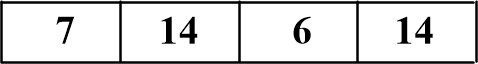
Figure 4: An example of an individual in the USS

An individual in the USS is an array of vertices whose the $i^{th}$ element is a vertex belonging the $i^{th}$ cluster in $G_{u}$. Figure 4 illustrate an individual in the USS which is created from the graph $G_{u}$ in Figure 3(e).

From this unified representation, we construct solutions for tasks through three main phases. Initially, a decoding phase is applied to find the private representation of the individual for each task. Afterward, the repairing phase will be conducted if needed in tasks so that a spanning tree can be built. Finally, a two-level construction strategy is conducted to build a CluSPT solution on the representation obtained after the above 2 phases. We will provide in-depth descriptions of the three phases in subsections 4.3, 4.4 and 4.5.

4.2 Individual Initialization Method

With the advantage of the individual representation in the form of an array of integers, as shown in subsection 4.1, the initialization, crossover, and mutation methods can be done easily and effectively. Each element in the individual is selected randomly from the cluster of the graph $G_{u}(V,C,m)$ built in the previous section. The initialization method details are presented in Algorithm 2 with time complexity of $O(m)$.

Input: Graph $G_{u}(V,C,m)$

Output: An individual in the USS

1 begin

2       $I\leftarrow\{\}$ ;

3       for k $\leftarrow$ 1 to m do

4             h $\leftarrow$ Random a vertex in $C^{k}$;

5             I $\leftarrow$ I $\cup$ {h};

6            

7       end for

8      return I;

9      

10 end

11

12

Algorithm 2 Initialization Individual Method

4.3 Proposed Decoding Method

This section describes a decoding method to construct an individual in each task from an individual in USS.

Each task’s individual is an integer array whose dimension equals the number of clusters in that task. The $i^{th}$ element is used to determine the local root of the $i^{th}$ cluster unless said cluster contains the source vertex of the input graph, in which case that source vertex will be the local root of the cluster. In all other cases, let $l$ be the vertex corresponding to the $i^{th}$ element. If $l$ can be found within the cluster, we make it the local root. Otherwise, we locate the maximum index of vertex $l$ among the $i^{th}$ clusters of all tasks. This is a guarantee due to the way we initialize the chromosome. We then take the vertex whose index is the remainder of the division between the maximum index found earlier and the cluster’s size. The method is described in Algorithm 3 with time complexity of $O(m^{2})$, where $m$ is the number of clusters.

Input:

• An input graph of the $i^{th}$ task $G_{i}(V_{i},E_{i},C_{i},C^{*}_{i},s_{i},m_{i})$, $C_{i}=\{C^{1}_{i},C^{2}_{i},...,C^{m_{i}}_{i}\}$ and $C^{*}_{i}=\{C^{1*}_{i},C^{2*}_{i},...,C^{m_{i}*}_{i}\}$.

• A graph $G_{u}(V,E,C,m)$.

• An individual in the USS $I=\{r_{1},r_{2},...,r_{m}\}$

Output: An representation of individual in space search of the $i^{th}$ task

1 begin

2       $Genes\leftarrow[]$;

3       for $j\leftarrow 1$ to $m_{i}$ do

4            

5            $l\leftarrow$ $r_{j}$ $\triangleright$ Value of the $j^{th}$ element in genes of individual $I$;

6             if vertex l doesn’t appear in $C^{j*}_{i}$ of $G_{i}$ then

7                   $p\leftarrow$ find maximum index of vertex $l$ in $C^{j*}_{h}$, $\forall h\in[1,\ldots,K]$ and ($h\neq i$);

8                   $size_{j}\leftarrow$ the number of elements in $C^{j*}_{i}$;

9                   $p\leftarrow$ $p\mod size_{j}$;

10                   $l\leftarrow$ value of the $p^{th}$ element in $C^{j*}_{i}$;

11                  

12             end if

13            $Genes$.append($l$);

14            

15       end for

16      return $Genes$;

17      

18 end

19

Algorithm 3 Proposed Decoding Method

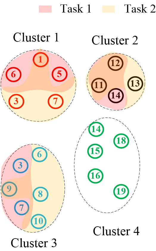
(a)

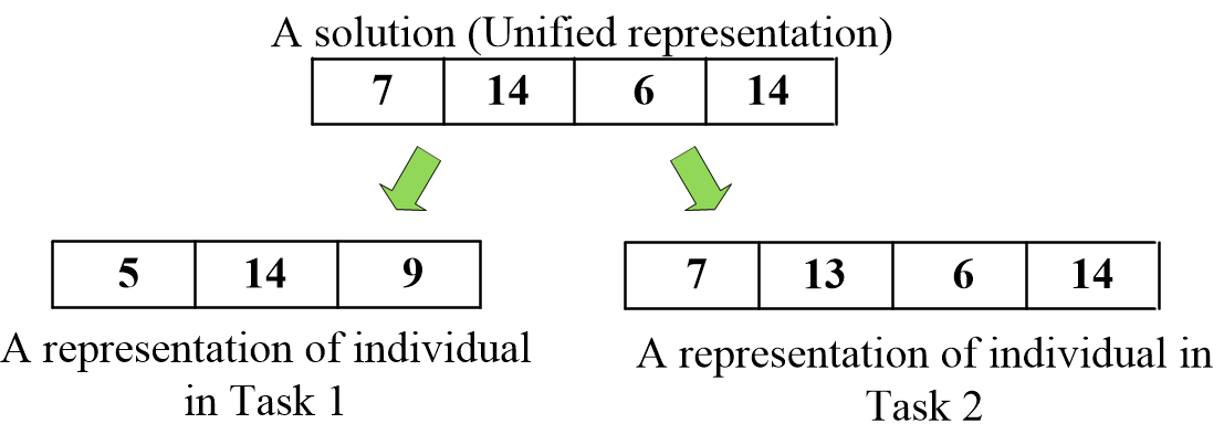
(b)

Figure 5: An example of steps of the decoding method to generate individuals for the tasks from an individual in USS

Figure 5 illustrates how the decoding method constructs the individuals in tasks $1$ and $2$ from the unified representation. Figure 5(a) provides a graph of the USS $G_{u}=(V,C,m)$ with 4 clusters ($m=4$). Sets of inter-vertices of clusters in Task 1 are $C^{1*}_{1}=\{1,6,5\}$, $C^{2*}_{1}=\{12,11,14\}$, $C^{3*}_{1}=\{9,7,3\}$ and in Task 2 are $C^{1*}_{2}=\{3,1,7\}$, $C^{2*}_{2}=\{11,12,13\}$, $C^{3*}_{2}=\{6,8,9,10\}$, $C^{4*}_{2}=\{14,15,16,18,19\}$, respectively. The decoding process for Task 1 is as follow. Vertex 7 doesn’t appear in $C^{1*}_{1}$ and the maximum index of vertex 7 in cluster 1 of other tasks (Task 2) is 2, so we choose a corresponding vertex to vertex 7 in the representation of Task 1. Vertex 5 is chosen since it has index $2$ ($=2\mod 3$) in cluster $C^{1*}_{1}$. Vertex 14 appears in $C^{2*}_{1}$, and thus it is added directly into the chromosome of Task 1. Vertex 6 doesn’t exist within $C^{3*}_{1}$ and its maximum index in cluster 3 of the other task is 0, therefore vertex 9 having index $0$ ( $=0\mod 3$) will be chosen as the corresponding vertex in the representation. As a result, a representation of Task 1 is constructed. The process for Task 2 is similar. In Figure 5(b), we demonstrate the two resulting individuals obtained after applying the decoding method.

4.4 Repairing Individual Method

Although the individual representation as the proposed encoding method has many advantages in storing, calculating, and executing evolutionary operators, it contains a weakness that can be exploited in incomplete graphs. Because the inter-vertices that are elected as the root of clusters are randomly selected, they may not guarantee connectivity between clusters and violate the local root properties. An example is depicted in Figure 6(a).

In this example, Figure 6(a) presents the input graph of the task, Figure 6(b) shows a representation of an individual obtained after the first decoding stage, which doesn’t guarantee local root properties of clusters. As shown in Figure 6(b), vertex 12, 8, and 19 are assigned to be the local root of clusters 2, 3, and 4, respectively. However, in the input graph, there is no path from 1 (source vertex) to 8 and 19, such that they must be the first visited vertices of their corresponding clusters, i.e., the local root property of the selected vertices cannot be guaranteed.

Therefore, a Repairing Individual Method (RIM) is introduced to fix this errors. Steps of RIM are as follows:

1. Add the cluster containing the source vertex to the closed set $V^{\prime}$.

2. Among the remaining clusters, RIM adds into $V^{\prime}$ all those whose local roots are connected to any vertex in $V^{\prime}$.

3. If there are still clusters outside of V’ after step 2 then do:

   1. Randomize an edge $(u,v)$ with $v\in V^{\prime}$ and $u\notin V^{\prime}$.

   2. Determine the cluster containing $u$ and change the local root of that cluster into $u$.

   3. Add vertices of that cluster to set $V^{\prime}$.

4. Repeat step 2 and step 3 until all clusters are added to $V^{\prime}$.

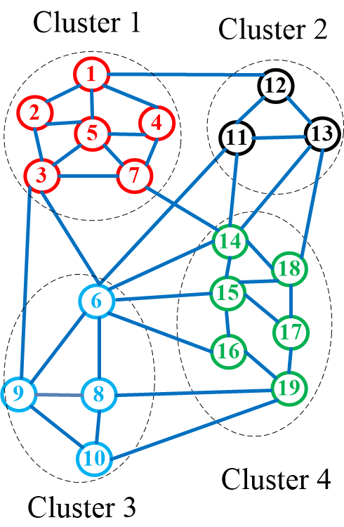
(a)

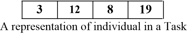
(b)

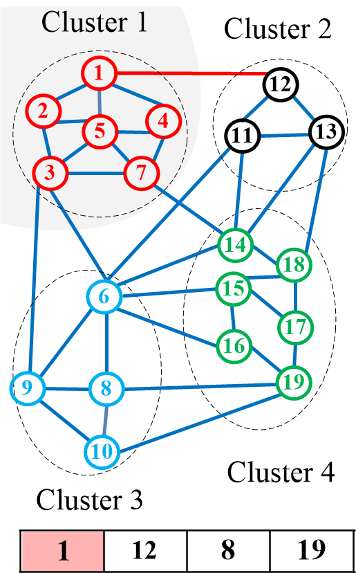
(c)

(d)

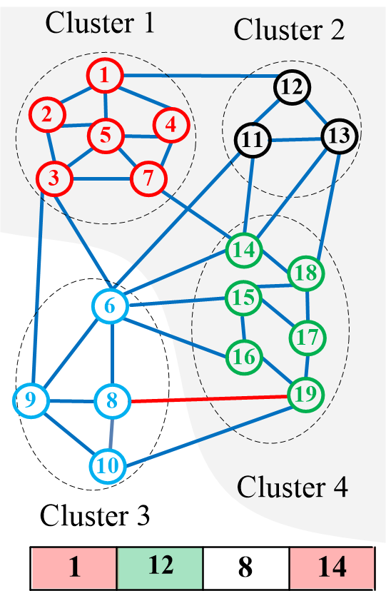
(e)

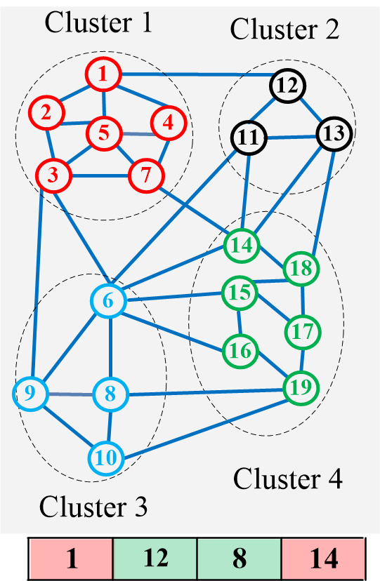
(f)

Figure 6: An example of steps to repair a individual representation

RIM’s implementation is presented in Algorithm 4. The algorithm’s time complexity is $O(m*|C^{\prime}|)$ where $m$, $C^{\prime}$ are the number of clusters and vertices set of the graph in the USS.

Input: An input graph of the $i^{th}$ task $G_{i}(V_{i},E_{i},C_{i},C^{*}_{i},s_{i},m_{i})$ where $C_{i}=\{C^{1}_{i},C^{2}_{i},...,C^{m_{i}}_{i}\}$, $C^{*}_{i}=\{C^{1*}_{i},C^{2*}_{i},...,C^{m_{i}*}_{i}\}$.

   An individual representation of the $i^{th}$ task $I=\{r_{1},r_{2},...,r_{m_{i}}\}$.

Output: A valid representation of $I$

1 begin

2       $C^{m}_{i}\leftarrow$ Determine the cluster containing the source vertex $s_{i}$ of $G_{i}$;

3       $I[m]\leftarrow$ $s_{i}$;

4       $C^{\prime}\leftarrow\{C^{1*}_{i}\cup C^{2*}_{i}\cup\ldots\cup C^{m_{i}*}_{i}\}$;

5       $V^{\prime}\leftarrow C^{m*}_{i}$ $\triangleright$ Add the cluster containing source vertex to set $V^{\prime}$;

6       $visited[r_{j}]\leftarrow false$ $\forall r_{j}\in I$ ;

7       $visited[s_{i}]\leftarrow true$;

8       $dem\leftarrow m_{i}-1$;

9      

10      while $dem>0$ do

11             existsEdge $\leftarrow$ false;

             /* Add clusters whose local root connects directly to at least one vertex in V’ to V’ */

12             foreach $r\in I$ do

13                   if ($visited[r]\neq true$) and ($\exists$ an edge $e=(r,k),k\in V^{\prime}$) then

14                         Determine cluster $C^{j*}_{i}$ containing vertex r ;

15                         $V^{\prime}\leftarrow V^{\prime}\cup C^{j*}_{i}$;

16                         $dem\leftarrow dem-1$;

17                         $visited[r]\leftarrow$ true;

18                         $existsEdge\leftarrow$ true;

19                         break;

20                        

21                   end if

22                  

23             end foreach

            /* If no remaining cluster has an explicit connection to at least one vertex in V’ through their local root, change the local root of a remaining random cluster */

24             if $existsEdge=false$ then

25                   Select randomly an edge $e=(h,k)$, $h\in V^{\prime}$ and $k$ $\in C^{\prime}\setminus V^{\prime}$;

26                   Determine cluster $C^{j*}_{i}$ containing vertex $k$;

27                   $V^{\prime}\leftarrow C^{j*}_{i}$;

28                   $dem\leftarrow dem-1$;

29                   Replace the local root of cluster $C^{j}_{i}$ in $I$ by the vertex $k$;

30                   $visited[k]\leftarrow$ true;

31                  

32             end if

33            return $I$;

34            

35       end while

36      

37 end

38

Algorithm 4 Repairing Individual Method

Figures 6(c)–6(f) describe how the RIM is carried out. The chromosome has been decoded for this task, and the designated local roots are 3, 12, 8, and 19. As vertex 3 is in the same cluster as the source vertex 1, 1 is chosen as the first cluster’s local root. In Figure 6(c), we add cluster 1 into $V’$ and now only cluster 2 is directly connected to $V^{\prime}$ through the edge (1,12) (highlighted in red). Thus, cluster 2 is added into $V^{\prime}$, as shown in Figure 6(d). Next, since both cluster 3 and 4 lack an explicit connection to $V^{\prime}$ from their local roots, we instead randomize an edge satisfies this condition. It can be seen that the edges (3, 6), (3, 9), (6, 11), (18, 13), (14, 7), (14, 13) and (11, 14) are eligible for selection. Let the edge (11, 14) be chosen, we change the local root of cluster 4 into 14 and add cluster 4 into $V^{\prime}$ (Figure 6(e)). Finally, we run through the clusters outside of $V^{\prime}$ again, in this case only cluster 3, and find that it is connected to $V^{\prime}$ using (8, 19). Cluster 3 is now added into $V^{\prime}$, and the resulting local roots are now guaranteed to produce a spanning tree.

Furthermore, to show RIM’s efficacy, we have provided and proven a lemma about the maximum number of positions to be fixed on the representation of each individual in Lemma 4.1.

Lemma 4.1.

The maximum number of positions that must be fixed on the genes is $\lfloor m/2\rfloor$ with $m$ is the size of genes.

Proof.

Assume that we construct a graph G by considering a cluster as a vertex. An edge between two vertices $v_{1}$ and $v_{2}$ exists in G if cluster 1 connects to cluster 2 via its local root or vice versa. Because each element in representation is an inter-vertex that always has at least an edge connecting to another cluster’s vertex (local root’s property), each vertex in G is always connecting to another vertex. Therefore, in the worst case, $G$ is a forest with $\lfloor m/2\rfloor$ connected components. To connect these connected components, it is necessary to modify one cluster’s local root in each component. For that reason, the maximum number of positions in the representation that need to be corrected is $\lfloor m/2\rfloor$. ∎

4.5 Construct a CluSPT solution for each task from representation of individual in its private search space

To evaluate an individual in a task, we need to construct a CluSPT solution based on that individual. Therefore, this section describes a method (called (CSC)), which builds a CluSPT solution effectively from the corresponding individual in the task. The CSC method consists of two levels as follows:

• We will build the shortest path tree in each cluster of the graph from the local root of each cluster. The set of edges obtained is added to the set of edges of the solution in the task.

• We will build the connecting edges between the clusters by using a customized version of Dijkstra’s algorithm. First, we add the entire set of vertices of the cluster containing the source vertex into a closed set $V$. Then we browse through the local root of the remaining clusters. Among the clusters connected to $V$ through their local roots, we search for the minimum route between a local root and the source vertex of the input graph. The cluster containing that root is then added to $V$, and the connecting edge is added to the edge set of the solution. Repeat until all clusters have been added to $V$.

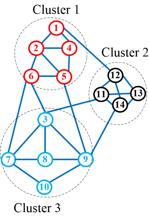
(a)

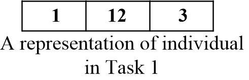
(b)

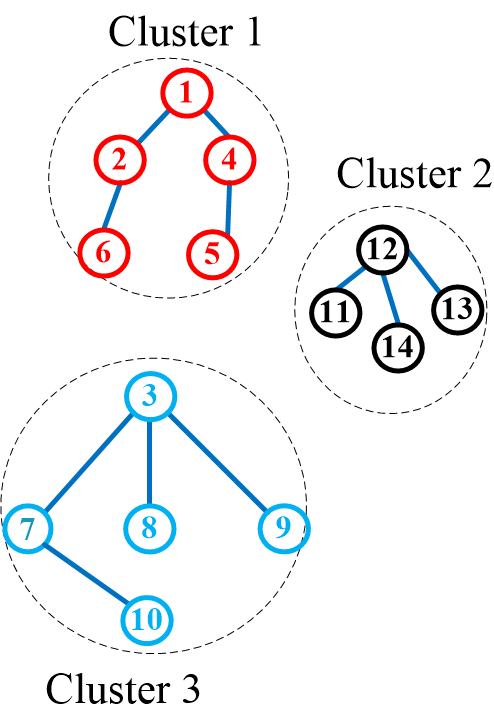
(c)

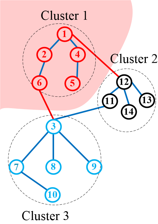
(d)

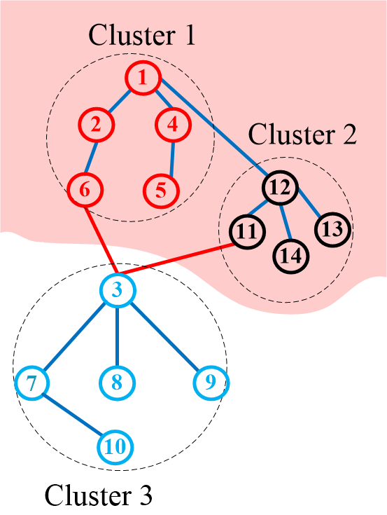
(e)

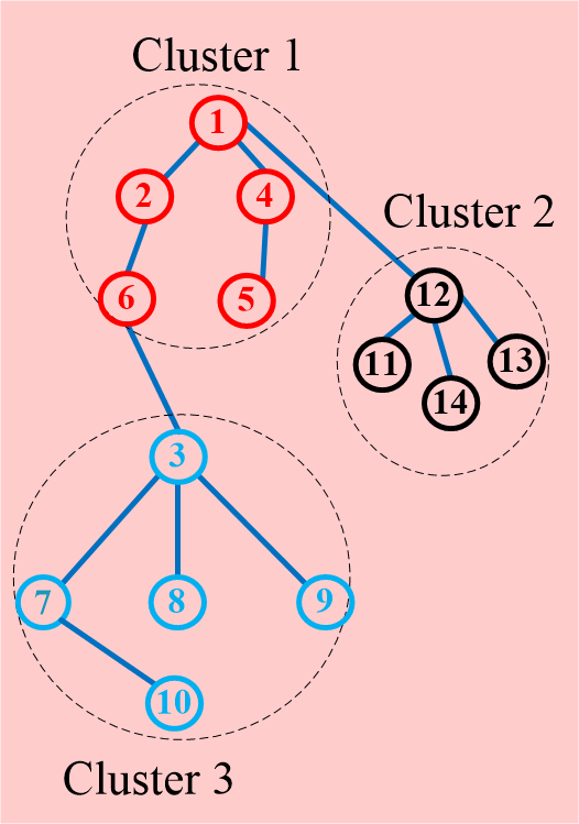
(f)

Figure 7: Steps to construct a solution from the private individual representation in the task

The steps of the CSC is described in Algorithm 5. The Dijkstra’s algorithm in the paper is implemented using the Binary Heap structure and its complexity when running on the input graph $G(V,E)$ is $O(E+V*logV)$. So for $m_{i}$ runs on $m_{i}$ clusters of graph will cost $O(m_{i}*(E^{\prime}+V^{\prime}*log(V^{\prime})))$ where $E^{\prime}$, $V^{\prime}$ are edges and vertices set of the largest cluster in the graph. In addition, the cost to build inter-cluster edges in $T$ is $O(m_{i}*V^{\prime})$. Therefore, the complexity of the whole Algorithm 5 is $O(m_{i}*(E^{\prime}+V^{\prime}+V^{\prime}log(V^{\prime})))$.

Input: An input graph of the $i^{th}$ task $G_{i}(V_{i},E_{i},C_{i},s_{i},m_{i})$, $C_{i}=\{C^{1}_{i},C^{2}_{i},...,C^{m_{i}}_{i}\}$ and $C^{*}_{i}=\{C^{1*}_{i},C^{2*}_{i},...,C^{m_{i}*}_{i}\}$.

   An individual $I=\{r_{1},r_{2},..,r_{m_{i}}\}$

1

Output: A spanning tree $T(V,E)$ and sum of routing cost ($sum$)

2 begin

3       $C^{m}_{i}\leftarrow$ Determine the cluster containing source vertex $s_{i}$ of $G_{i}$;

4       $V\leftarrow V_{i}$;

5       $E\leftarrow\emptyset$;

6       $sum\leftarrow$ 0 $\triangleright$ the total routing cost from source vertex $s_{i}$ to all vertices in T;

       /* Construct the shortest path tree in each cluster from its local root by Dijsktra Algorithm */

7       foreach cluster $C^{j}_{i}\in\mathcal{C}_{i}$ do

8             $T_{j}\leftarrow$ Determine the shortest path tree for $G_{i}[C^{j}_{i}]$ from local root $r_{j}$;

9             $d_{r_{j}k}\leftarrow$ the cost of path from the local root $r_{j}$ to a vertex $k\in$ $C^{j}_{i}$ in $T_{j}$;

10             $sum\leftarrow sum$ + $\sum d_{r_{j}k},\forall k\in C^{j}_{i}$;

11             $E\leftarrow E\cup E(T_{j})$;

12            

13       end foreach

14      

      /* Construct edges connecting among clusters in T */

15       $V^{{}^{\prime}}\leftarrow C^{m*}_{i}$;

16       $visited[r_{j}]\leftarrow$ false;

17       $cost[r_{j}]\leftarrow\infty,\forall r_{j}\in I$ $\triangleright$ $cost[r_{i}]$ is the minimum cost to join the $j^{th}$ cluster into T through its local root $r_{i}$;

18       $visited[s_{i}]\leftarrow true$;

19       $dem\leftarrow m_{i}-1$;

       /* Join cluster having the smallest additional cost */

20       while $dem>0$ do

21             min $\leftarrow\infty$;

22             $v,u\leftarrow$ $null$;

23             foreach $r\in I$ do

24                   if  $visited[r]\neq true$ then

25                         foreach edge e=(r, k), k $\in$ V’ do

26                               $n_{cr}\leftarrow$ the number of vertices in the cluster contain $r$;

27                               $cost[r]$ $\leftarrow$ min($cost[r]$, ($d_{s_{i}k}$ + $c(k,r))*n_{cr}$);

28                               if  $cost[r]<min$ then

29                                     min $\leftarrow$ $cost[r]$; u $\leftarrow$ r;

30                                     v $\leftarrow$ $arg\_min(cost[r])$;

31                                    

32                               end if

33                              

34                         end foreach

35                        

36                   end if

37                  

38             end foreach

39            sum $\leftarrow$ sum + $cost[u]$ $\triangleright$ Update the total routing cost;

40             Determine cluster $C^{j}_{i}$ containing vertex $v$ and update routing cost from source vertex $s_{i}$ to vertices in $C^{j}_{i}$;

41             $V^{\prime}\leftarrow$ $C^{j*}_{i}$;

42             $E\leftarrow$ $E\cup(u,v)$;

43             $dem\leftarrow dem-1$;

44             $visited[u]\leftarrow$ true;

45            

46       end while

47      return T(V, E), sum;

48      

49 end

50

Algorithm 5 Construct the Solution of CluSPT

Figure 7 presents a process of constructing the solution from the private representation of an individual in task $T_{1}$. Figure 7(a) shows the clusters of a task within the MFEA and in the Figure 7(b), we see its individual representation. Vertex 1 is the source vertex of the input graph. Going through the chromosome, we get the three local roots: 1, 12, and 3. In the Figure 7(c) internal trees are created inside the clusters. We add the cluster containing source vertex 1 into $V$, as shown in Figure 7(d). Next, we consider all the clusters that connect directly to $V$, in this case, both local roots 12 (through vertex 1) and 3 (through vertex 6). Comparing these two routes, we see that routing from 12 to 1 is closer than from 3 to 1, and thus cluster 2 is added to $V$ (figure 7(e)). Finally, cluster 3 is connected to $V$ through both 6 and 11. Since the path $3\rightarrow 6\rightarrow 1$ is shorter than the path $3\rightarrow 11\rightarrow 1$, we add cluster 3 into $V$ and the edge (3, 6) into the set of edges.

4.6 Crossover Operator

In traditional MFEA, the new children are produced from two parents who have the same skill factor or satisfy a random probability. In our proposed crossover operator (New Multi-Parent Crossover (N-MPCX)), the parents have the same choice, but their children are produced from more parents in the hope that they could inherit much more characteristics of trees of their parent. This is similar to how farmers breed new crops that inherit the good traits of more than two-parent trees: good pest resistance of plant A, high yield of plant B, good fruit quality of plant C, etc.

The N-MPCX as shown in Algorithm 6 and its time complexity is $O(N*m)$ with $N$, $m$ are number of parents and the number of genes.

Figure 8 shows offsprings obtained after performing N-MPCX’s steps. Figure 8(a) presents 4 $(N=4)$ input parents and $N-1=4-1=3$ cut points selected randomly. The $i^{th}$ offspring preserves two segments of genes which are from the $(i-1)^{th}$ cut point to $i^{th}$ cut point and $(N-1)^{th}=3^{rd}$ cut point to the end of its corresponding parent. Other segments of the offsprings is determined by the gene segment of their next parents in order. If the segment selected is from $(i-1)^{th}$ cut point to $i^{th}$ cut point of the $i^{th}$ parent then change it to the next parent’s gene segment in the same position. Figure 8(b) shows 4 offsprings obtained.

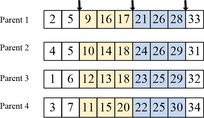
(a)

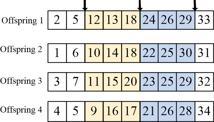
(b)

Figure 8: An example for the proposed crossover operator

Input: $N$ parents $P_{i}=\{p_{i1},p_{i2},...,p_{im}\}$, $i=1,\ldots,N$, $2\leq N\leq m$.

Output: $N$ offsprings $O_{i}$, $i=1,\ldots,N$

1 begin

2       if $N=2$ then

3             $cp_{i}\leftarrow$ Select randomly two cut points where $1\leq cp_{i}\leq m$ ($i=1,2$), $cp_{1}<cp_{2}$;

4             $O_{i}$ $\leftarrow$ $P_{i}$, $i=1,2$;

5             Swap genes from $cp_{1}$ to $cp_{2}$ of two offsprings $O_{1},O_{2}$ for each other;

6            

7       else

8             $cp_{1},\ldots,cp_{N-1}\leftarrow$ Select randomly $N-1$ cut points where ($1\leq cp_{i}<cp_{i+1}\leq m-1$);

9             $idx\leftarrow$ 1 ;

10             for i $\leftarrow$ 1 to N-1 do

11                   for j $\leftarrow$ 1 to N do

12                         $h\leftarrow j$;

13                         if  $j\mod N+1=i$ then

14                               $h\leftarrow(j+1)\mod N+1$;

15                              

16                        if j $\neq$ i then

17                               h $\leftarrow$ $j\mod N+1$;

18                         Copy the gene segment from index $idx$ to $cp_{i}$ in parent $P_{h}$ and append them into Offspring $O_{j}$;

19                        

20                   end for

21                  $idx\leftarrow$ $cp_{i}+1$;

22                  

23             end for

24            for j $\leftarrow$ 1 to N do

25                   Copy the gene segment from index $idx$ to $m$ in parent $P_{j}$ and append them into Offspring $O_{j}$;

26                  

27             end for

28            

29       end if

30      return $O_{i}$, $i=1,\ldots,N$;

31      

32 end

33

Algorithm 6 Proposed crossover operator

4.7 Mutation operator

The mutation operator is performed by randomly selecting a cluster and replacing its local root with another inter-cluster vertex in that cluster. The mutation method is described in Algorithm 7 with time complexity is $O(1)$.

Input: The Graph $G_{u}(V,C,m)$ where $C=\{C^{1},C^{2},..,C^{m}\}$,

   An individual $I=\{r_{1},r_{2},..,r_{m}\}$

. Output: A new individual $I^{*}=\{r^{*}_{1},r^{*}_{2},..,r^{*}_{m}\}$

1 begin

2       $I^{*}\leftarrow I$;

3       k $\leftarrow$ Choose a random position in $I$;

4       ${r^{\prime}}_{k}\leftarrow$ Choose a random vertex in cluster $C^{k}$;

5       $r^{*}_{k}\leftarrow{r^{\prime}}_{k}$;

6       return $I^{*}$;

7      

8 end

9

Algorithm 7 Proposed mutation operator

4.8 New method to speed up the evaluation for the CluSPT solution

Given a spanning tree $T$ is a solution of the CluSPT problem, the cost of the solution as defined is the sum of the shortest path distances from the source vertex $s$ to all the vertices in the tree:

$$\begin{split}cost(T)&=\sum_{u\in V}d_{T}(s,u)\\ &=\sum_{i=1}^{m}\sum_{v\in C^{i}}d_{T}(s,v)\\ &=\sum_{i=1}^{m}\sum_{v\in C^{i}}\left(d_{T}(s,r_{i})+d_{T}(r_{i},v)\right)\\ &=\sum_{i=1}^{m}\left(|C^{i}|*d_{T}(s,r_{i})+\sum_{v\in C^{i}}d_{T}(r_{i},v)\right)\\ \end{split}$$ (1)

From the above formula after decomposition, it can be easily seen that to calculate the cost of the solution, we need to calculate two components:

• The cost of path from source vertex $s$ to the local root vertices of clusters $r_{i}$: $d_{T}(s,r_{i}),i=1,\ldots,m$.

• The sum of costs of the path from the local root $r_{i}$ of each cluster to all vertices in that cluster $\sum_{v\in C^{i}}d_{T}(r_{i},v)$.

In the above equation, the second component $\sum_{v\in C^{i}}d_{T}(r_{i},v)$ does not depend on the source vertex $s$, but only on the local root and the subgraph of that cluster. And the result of this component can be determined by Dijkstra’s algorithm once we know the local root $r_{i}$ of that cluster. Therefore, to increase the algorithm’s speed, we only calculate this value of each cluster for each local root only once on the first calculation and save it to memory. When later calculation with the same local root is called, the corresponding memory cell’s value will be retrieved. This saves a lot of computational costs because the cost of each Dijkstra’s algorithm implementation is quite expensive. And this is also the reason why the idea of the encoding method is only based on the local root of each cluster in this paper is generated.

5 Computational results

5.1 Problem instances

To the best of our knowledge, there have been no instances of the CluSPT made available to the public. For this reason, a set of test instances based on the MOM [24] (called MOM-lib) is generated. Various algorithms are utilized in the MOM-lib [25], resulting in six distinct types of instances. They are categorized into two kinds regarding dimensionality: small instances, each of which has between 30 and 120 vertices, and large instances, each of which has over 262 vertices. The instances are suitable for evaluating cluster problems [24].

However, to test the proposed algorithms’ effectiveness in solving the CluSPT, it is necessary to add information about a source vertex to each instance. Therefore, a random vertex is selected as the source vertex for each instance.

For evaluation of the proposed algorithms, instances with dimensionality from 30 to 500 are selected. All problem instances are available via [26].

5.2 Experimental criteria

Criteria for assessing the quality of the output of the algorithms are presented in Table 1.

Table 1: Criterias for assessing the quality of the output of the algorithm

Average (Avg)	The average function value over all
Best-found (BF)	Best function value achieved over all runs
Relative Percentage Differences (RPD)	The difference between the average costs of two algorithms

In order to compare the quality of the CluSPT solutions received from distinct algorithms, RPD [27] is used to calculate the difference between the average costs of two algorithms. The RPD is calculated by the following formula:

$$RPD=\dfrac{Solution-Best}{Best}*100\%$$

, where $Best$ is the average cost of the solution obtained from the proposed algorithm, $Solution$ is the average cost of the solution obtained from existing algorithms, including Heuristic Based on Randomized Greedy Algorithm (HB-RGA) and a strategy for using multifactorial optimization (G-MFEA).

The experimental results were recorded in tables given at the end of this paper. Each table was labeled with the numbers on the instances’ types.

5.3 Experimental setup

To evaluate the performance of new MFEA for the CluSPT, two sets of experiments are implemented.

• On the first set, two recent algorithms, G-MFEA [12] and HB-RGA [28] were implemented.

• On the second set, since the performance of the proposed MFEA were contributed by parameter: the relation between the number of vertices and the number of clusters, R-experiment is conducted to evaluate the effect of these parameters.

Each scenario was simulated 30 times on the computer (Intel Core i7 - 4790 - 3.60GHz, 16GB RAM), with a population size of 100 individuals evolving through 500 generations, which means the total numbers of task evaluations are 50000, the random mating probability is 0.5, and the mutation rate is 0.05. The source codes were installed by Java language.

5.4 Experimental results

To demonstrate the effectiveness of the proposed algorithm, we perform three analyses on the received results:

• Statistical tests that have become a widespread technique in computational intelligence are first used to analyze the algorithms’ performance.

• The details of comparison on each type of instance is discussed in the second analysis.

• In the third analysis, we point out factors that impact the performance of the proposed algorithm in comparison with existing algorithms.

5.4.1 Non-parametric statistic for comparing the results of proposed algorithm and existing algorithm

In order to examine the effect of the algorithms New Multifactorial Evolutionary Algorithm (K-MFEA), HB-RGA, and G-MFEA on the obtained results, we use Non-parametric for analyzing the received results. This study has two main steps:

• The first step uses statistical methods such as Friedman, Aligned Friedman, Quade [29, 30] to test the differences among the results obtained by each algorithm.

• The second step is performed when the test in the first step rejects the hypothesis of equivalence of means, the detection of concrete differences among the algorithms can be made with the application of post-hoc statistical procedures [29, 30], which are methods used for comparing a control algorithm with remaining algorithms.

Tables LABEL:tab:ResultsType1-LABEL:tab:ResultsType6 present the results obtained in the competition organized by types of instances and three algorithms. In these tables, the italic, red cells on a column in an algorithm denote instances where this algorithm outperforms two other algorithms.

Table 2: Results of the Friedman and Iman-Davenport test ($\alpha$=0.05)

Friedman Value	Value in $X^{2}$	$p$-value	Iman-Davenport Value	Value in $F_{F}$	$p$-value
175.353	5.991	$9.869*10^{-11}$	235.745	3.028	$1.940*10^{-60}$

The result of applying Friedman’s and Iman-Davenport’s tests is presented in Table 2. Given that the statistics of Friedman and Iman-Davenport are greater than their associated critical values, there are significant differences among the observed results with a probability error of $p\leq 0.05$.

Table 3: Average rankings achiedved by the Friedman, Friednman Aligned, and Quade tests

Algorithms	Friedman	Friednman Aligned	Quade
HB-RGA	2.669	273.831	2.600
G-MFEA	2.209	230.939	2.323
K-MFEA	1.122	122.230	1.076

Table 3 summarizes the ranking obtained by the Friedman, Friedman Aligned, and Quade tests. Results in Table 3 strongly suggest the existence of significant differences among the algorithms considered.

The results in Table 3 show that the rank of the K-MFEA algorithm is the smallest, so we choose K-MFEA as the control algorithm. After that, we will apply more powerful procedures, such as Holm’s and Holland’s, to compare the control algorithm with the other algorithms. Table 4 shows all the possible hypotheses of comparison between the control algorithm and the remaining ones, ordered by their $p$-value and associated with their level of significance.

Table 4: The z-values and p-values of the Friedman Aliged, Quade procedures (K-MFEA is the control algorithm)

		Friedman				Quade
$i$	algorithms	$z$	$p$	Holm	Holland	$z$	$p$	Holm	Holland
2	HB-RGA	12.89	$4.81*10^{-38}$	0.025	0.025	11.02	$2.79*10^{-28}$	0.025	0.025
1	G-MFEA	9.05	$1.35*10^{-19}$	0.05	0.05	9.02	$1.85*10^{-19}$	0.05	0.05

Table 5 and Table 6 show all the adjusted $p$ values for each comparison which involves the control algorithm. The $p$ value is indicated in each comparison, and we stress in bold the algorithms which are worse than the control algorithm, considering a level of significance $\alpha=0.05$.

Table 5: Adjusted p-values for the Friedman test (K-MFEA is the control method)

i	Algorithms	Unadjusted $p$	$p_{Bonf}$	$p_{Holm}$	$p_{Hochberg}$	$p_{Pli}$
1	HB-RGA	$4.81*10^{-38}$	$9.62*10^{-38}$	$9.62*10^{-38}$	$9.62*10^{-38}$	$4.81*10^{-38}$
2	G-MFEA	$1.34*10^{-19}$	$2.70*10^{-19}$	$1.34*10^{-19}$	$1.34*10^{-19}$	$1.34*10^{-19}$

Table 6: Adjusted p-values for the QUADE test (K-MFEA is the control method)

i	Algorithms	Unadjusted $p$	$p_{Bonf}$	$p_{Holm}$	$p_{Hochberg}$	$p_{Pli}$
1	HB-RGA	$2.79*10^{-28}$	$5.59*10^{-28}$	$5.59*10^{-28}$	$5.59*10^{-28}$	$1.84*10^{-28}$
2	G-MFEA	$1.85*10^{-19}$	$3.70*10^{-19}$	$1.85*10^{-19}$	$1.85*10^{-19}$	$1.85*10^{-19}$

5.4.2 Detail of comparison among the algorithms K-MFEA, HB-RGA and G-MFEA

*) The aspect of solution quality

Tables 7 summarize the results obtained in comparison with two other algorithms. The results show that K-MFEA is significantly superior to HB-RGA. K-MFEA exceeds HB-RGA on most instances in all types, while the result received by HB-RGA is equal to one received by K-MFEA on only an instance in Type 5 small. Between G-MFEA and K-MFEA, there are 29 test cases where the two algorithms’ performance is equally matched. Combined with the results on Tables LABEL:tab:ResultsType1-LABEL:tab:ResultsType6, we can see that a highlight in those test cases is the dimension of instances are often small, i.e., the dimension of instances in Type 1, Type 5, and Type 6 are less than 76, 65 and 76, respectively. G-MFEA outperforms K-MFEA on two instances which are instance 5i500-304 in Type 5 Large and instance 9pr439-3x3 in Type 6 Large. However, K-MFEA surpasses G-MFEA on 108 out of 139 instances. Particularly, results obtained by the proposed algorithm are better than ones obtained by G-MFEA in all instances in Type 1 Large and Type 3.

Table 7: Summary of comparison of results obtained by K-MFEA and the existing algorithms.

		K-MFEA
		outperforms G-MFEA	is equal to G-MFEA	outperforms HB-RGA	is equal to HB-RGA	Total
Type 1	Small	18	8	26	0	26
	Large	15	0	15	0	15
Type 3		5	0	5	0	5
Type 4		6	4	10	0	10
Type 5	Small	10	10	19	1	20
	Large	14	0	15	0	15
Type 6	Small	28	7	35	0	35
	Large	12	0	13	0	13

The average RPD and the maximum RPD of K-MFEA in comparison with G-MFEA and HB-RGA on types are presented in Figure 9, in which the labels G-MFEA and HB-RGA mean RPD(K-MFEA, G-MFEA) and RPD(K-MFEA, HB-RGA) respectively.

In Figure 9(a), we can observe the average RPD(K-MFEA, G-MFEA) is larger than the average RPD(K-MFEA, HB-RGA) on Type 6 small, Type 4 and both small and large instances on Type 1, and the biggest difference is on Type 4. The average RPD(K-MFEA, G-MFEA) in those types are of 4.4%, 2.4% and 4.1% respectively. Conversely, the average RPD(K-MFEA, G-MFEA) is smaller than the average RPD(K-MFEA, HB-RGA) on other types, in which the average RPD(K-MFEA, HB-RGA) reaches its highest on Type 3 with the value of 2.2% and its lowest on Type 5 small with the value of 1.1%. Another remarkable point in Figure 9(a) is that on Type 5 Small, the average RPD(K-MFEA, G-MFEA) is very low with the value of 0.04%. It mean that on this type, the improvement of performance of K-MFEA is significantly small in comparison with G-MFEA. The reason behind this is that the dimension of instances on this type is small, leading to the difference between the two algorithms not being large.

Figure 9(b) indicates that the biggest gap between K-MFEA and G-MFEA is significantly larger than one between K-MFEA and HB-RGA, and the maximum RPD(K-MFEA, G-MFEA) peaked at 18.6% on Type 4. A notable point in this figure is that the smallest gaps also belong to RPD(K-MFEA, G-MFEA) with value of 0.32% (Type 3), 0.3196% (Type 5 small) and 0.334% (Type 6 large). Smaller difference in this scene denotes that in comparison with K-MFEA, the results obtained by G-MFEA are closer than ones obtained by HB-RGA. In other words, in comparison with G-MFEA, the solution quality produced by K-MFEA is not significantly improvement on these types.

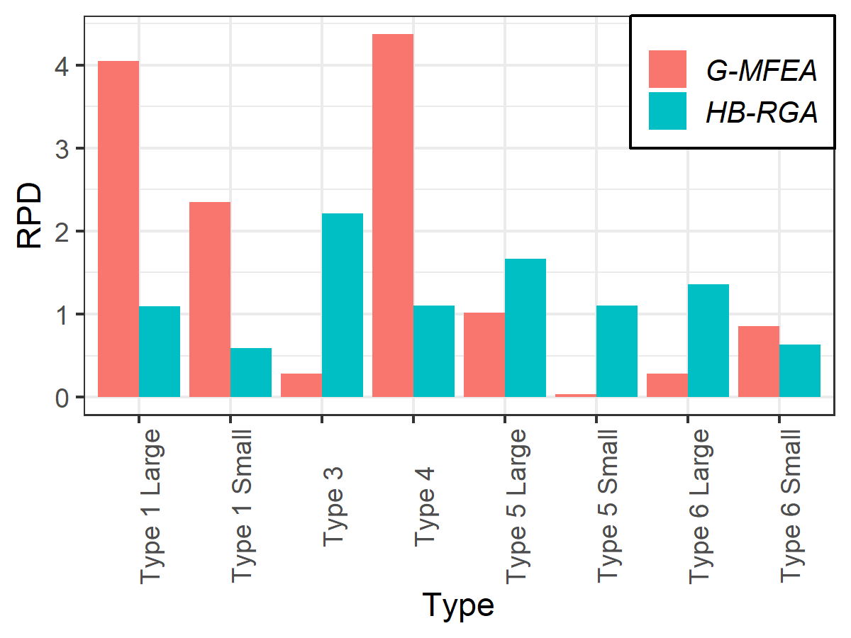
(a) Average RPD

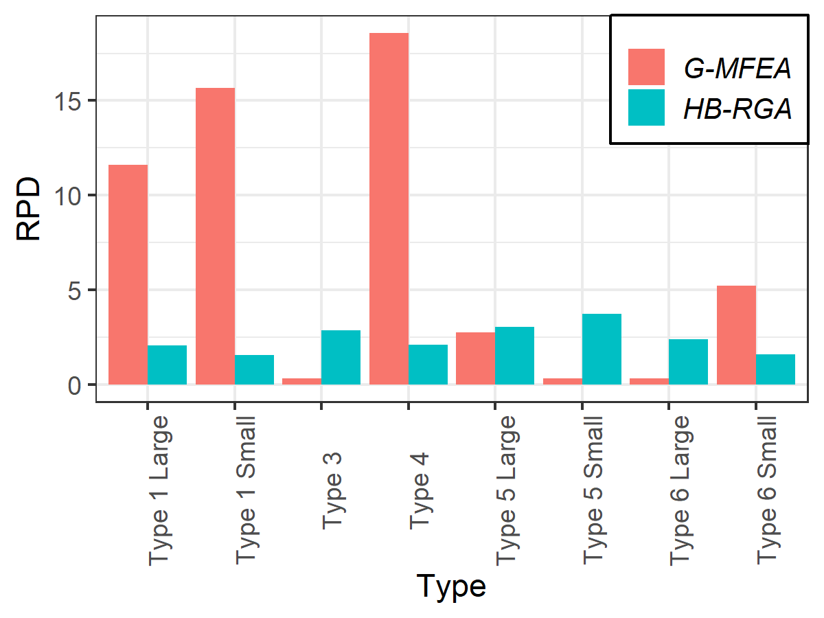
(b) Maximum RPD

Figure 9: Average RPD and maximum RPD of K-MFEA in comparison with G-MFEA and HB-RGA on types

*) The aspect of running time

Figure 10 depicts the average running time, in minutes, of the three algorithms. It can be seen quite clearly that G-MFEA is the inferior algorithm in this regard, compare to both HB-RGA and K-MFEA. As such, the focus should be shifted to a comparison between HB-RGA and K-MFEA, represented by Figure 11. For the small instances (Type 1 Small, Type 5 Small, Type 6 Small), K-MFEA achieves an execution time about 1.4-2 times faster than HB-RGA. Excluding those types, however, K-MFEA has proven itself to be the superior method as HB-RGA runs at least 6 times slower. This difference cannot be attributed alone to the nature of the K-MFEA and MFEA algorithms, which solve multiple problems at once, because G-MFEA too utilizes the MFEA model and loses out horribly on running time. A better explanation for this is the speed up method covered in this paper (section 4.8), which massively reduces computational stress.

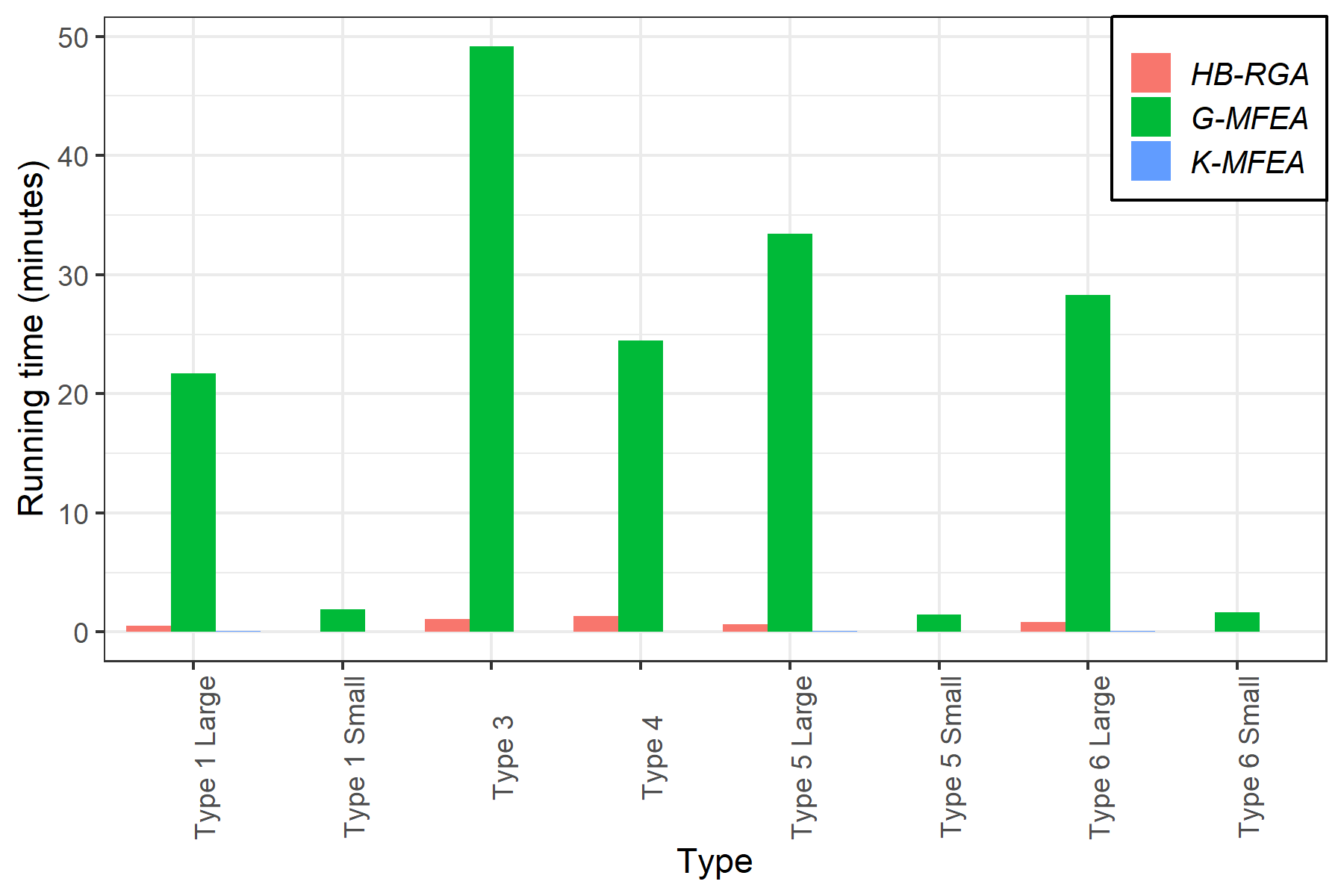
Figure 10: Running time of K-MFEA, G-MFEA and HB-RGA on types

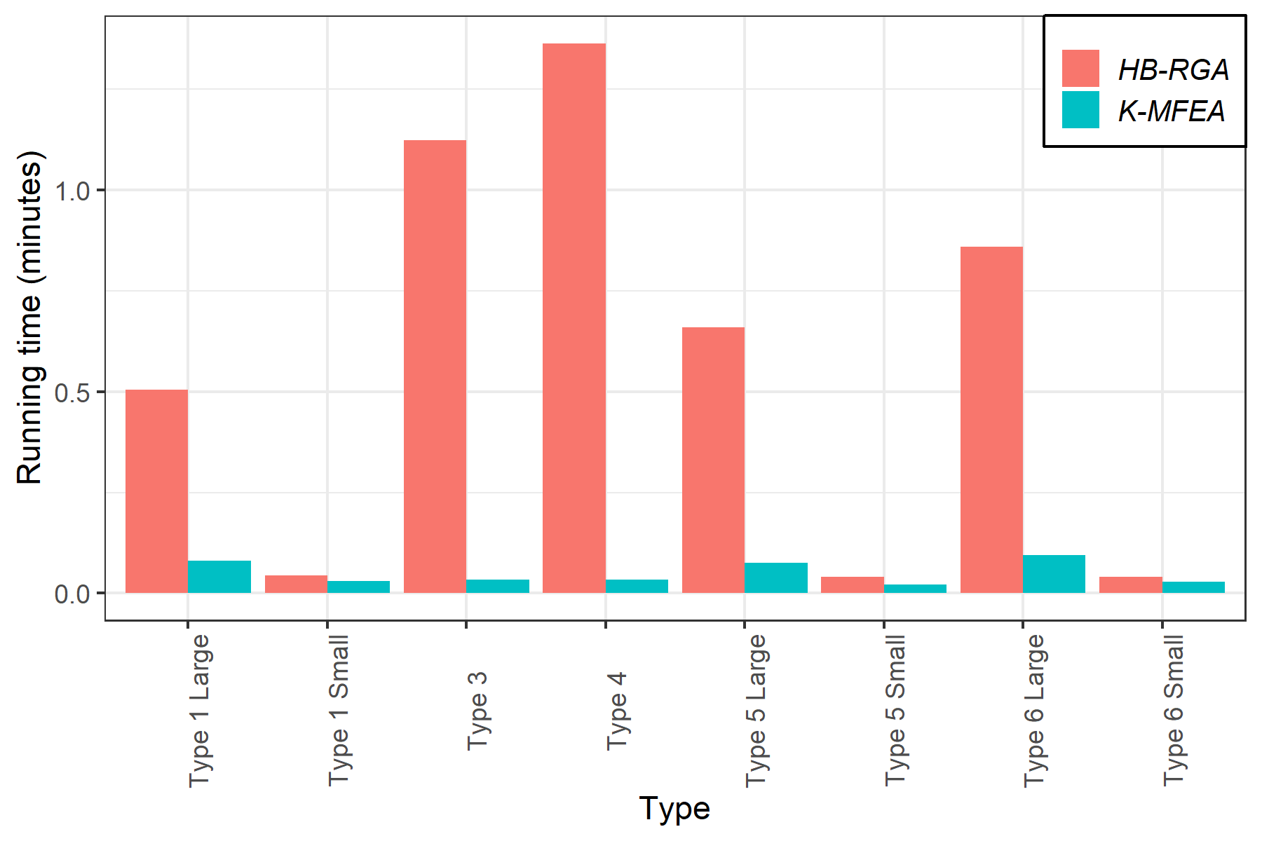
Figure 11: Running time of K-MFEA in comparison with HB-RGA on types

5.4.3 Analysis of influential factors

As mentioned in the previous subsection, the number of vertices may affect the performance of the K-MFEA. Therefore, In this subsection, the influence of the input graph’s dimension (the number of vertices) on the performance of K-MFEA is analyzed. Because K-MFEA outperforms both G-MFEA and HB-RGA on all instances of Type 3 and the number of instances in Type 4 is also very small, this study only considers the instances of Type 1, Type 5, and Type 6.

In the previous subsection, the results have proven that K-MFEA surpasses HB-RGA in most test cases, i.e., on 138 out of 139 instances, so we only focus on analyzing the performance of K-MFEA in comparison with G-MFEA.

To determine the correlation between the number of vertices, the scatter plots of the relationship between the number of vertices and the comparison between two algorithms K-MFEA and G-MFEA for each type are graphed, and then this study tries to find the correlation coefficient in that relationship as shown in Figure 12. In these Figures, circle symbols represent the performance of K-MFEA over G-MFEA, triangle means that the performance of G-MFEA outperforms K-MFEA, and square symbols illustrate the performance of the two algorithms when they are equal.

Figure 12 describes the relationship between the number of clusters and the performance comparison between K-MFEA and G-MFEA. A common feature of these figures is that the results from two algorithms are equal when the number of vertices is small, i.e., Type 1, Type 5, Type 6 is smaller than 76, 30, and 76, respectively. When the number of vertices is greater than 76 (for Type 1 and Type 6) and 30 (for Type 5), G-MFEA exceeds K-MFEA on only two test cases, which are on instance 5i500-304 in Type 5 and instance 9pr439-3x3 in Type 6. These lead to the conclusion that when the input graph’s dimension increases, the performance of K-MFEA tends to increase.

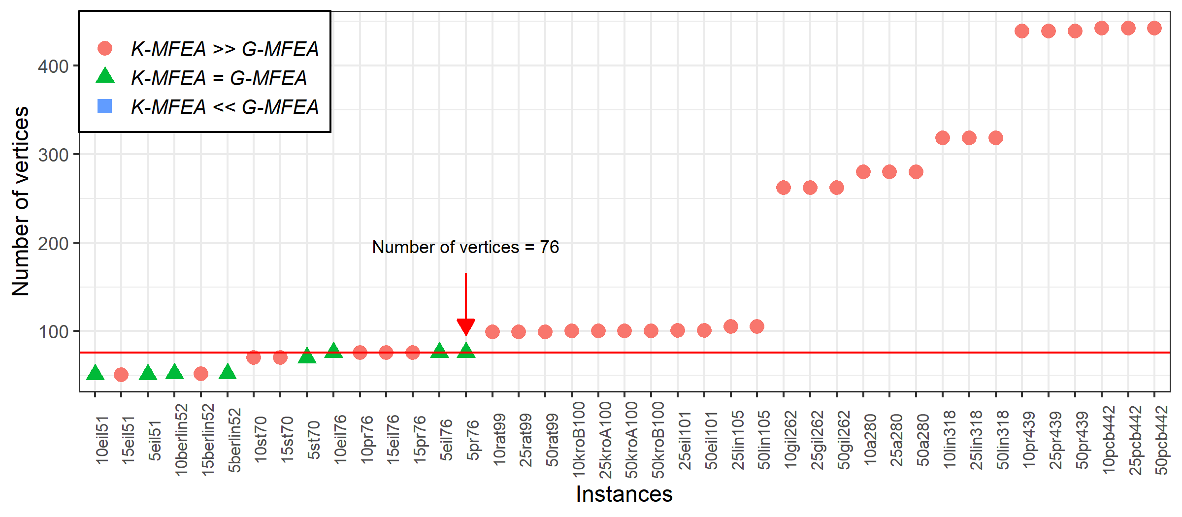
(a) Type 1

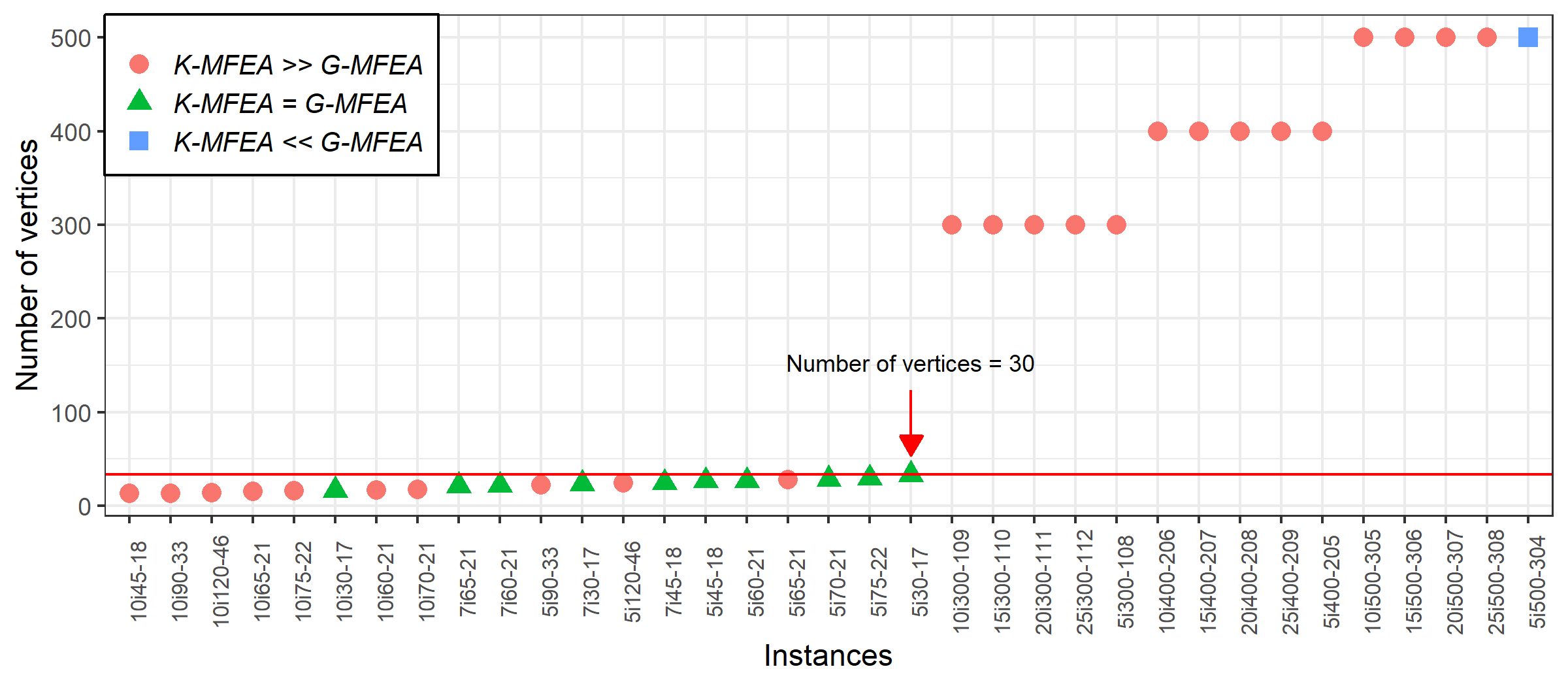
(b) Type 5

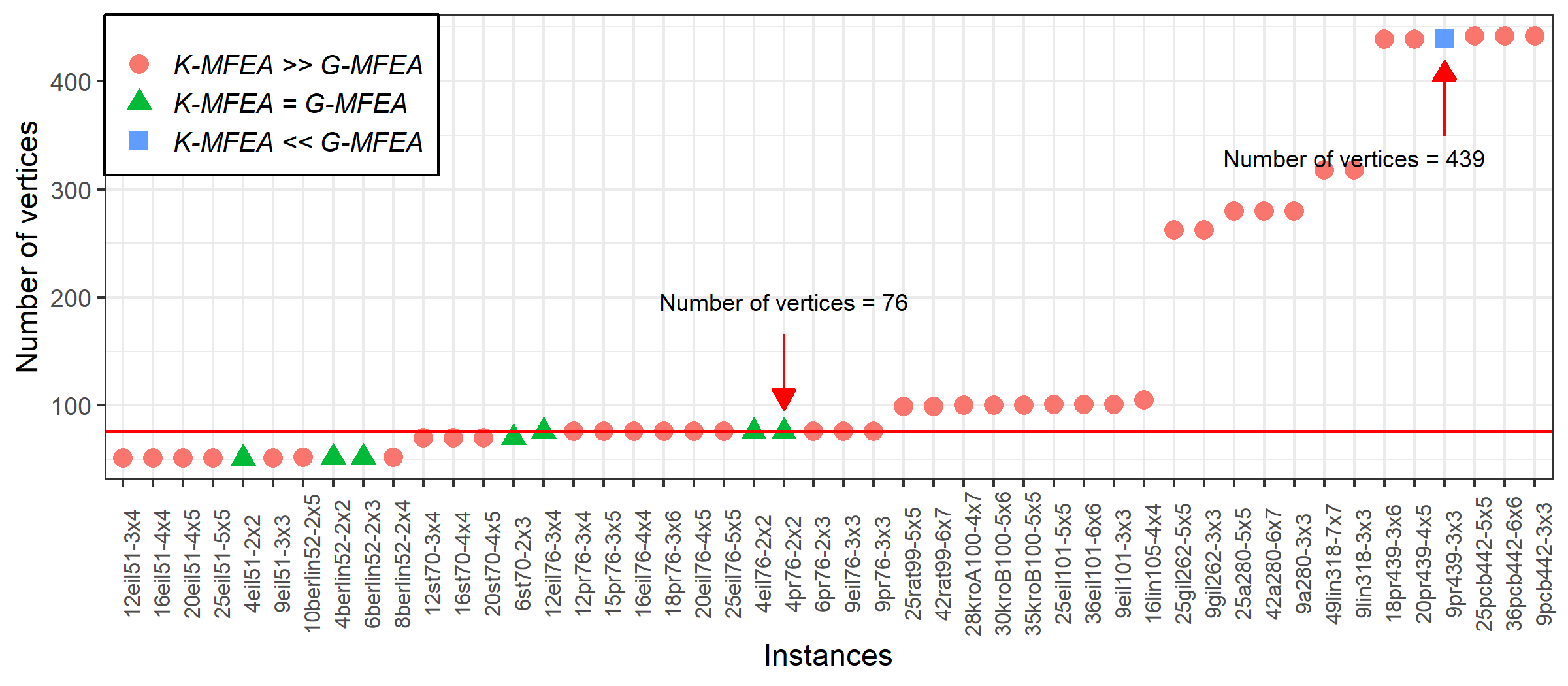
(c) Type 6

Figure 12: The scatter of the number of vertices and the comparison between K-MFEA with G-MFEA in the Types 1, 5 and 6

5.4.4 Convergence trends

In order to better understand the improved performance as a result of the proposed algorithm, we analyze the convergence performance of two algorithms G-MFEA and K-MFEA by using the functions in [17] for computing the normalized objectives and averaged normalized objectives of the algorithms. In each type, a pair of instances are randomly selected for performing the analysis.

Figure 13 illustrates the main convergence trends during the initial stages of K-MFEA and G-MFEA for instances 10pr439 and 25a280 in Type 1; instances 5i300-108 and 5i400-205 in Type 5, and instances 9pcb442-3x3 and 9pr439-3x3 in Type 6. From Figure 13 it can be noted that in general, the convergence trend of K-MFEA converges faster than one of K-MFEA and can categorize into two major trends:

• The convergence trend of K-MFEA also surpassed that of G-MFEA on all generators as in Figure 13(a).

• The convergence trend of K-MFEA surpasses that of G-MFEA on the last generators but on the first generators, the convergence of G-MFEA was often faster than that of K-MFEA. This trend is illustrate in Figure 13(b) and Figure 13(c).

One other remark in Figure 13 is the average normalized objective values difference between K-MFEA and G-MFEA at start time. The cause of this difference is that two algorithms encode the CluSPT solution by two different methods, so initial individuals of an algorithm differ from initial solutions of the rest algorithm. These observations led to the conclusion that the CluSPT solution produced by K-MFEA was often better than ones produced by G-MFEA in most generators. In other words, the evolution methods in K-MFEA may help to improve the quality of solution of the CluSPT in comparison with the methods in G-MFEA.

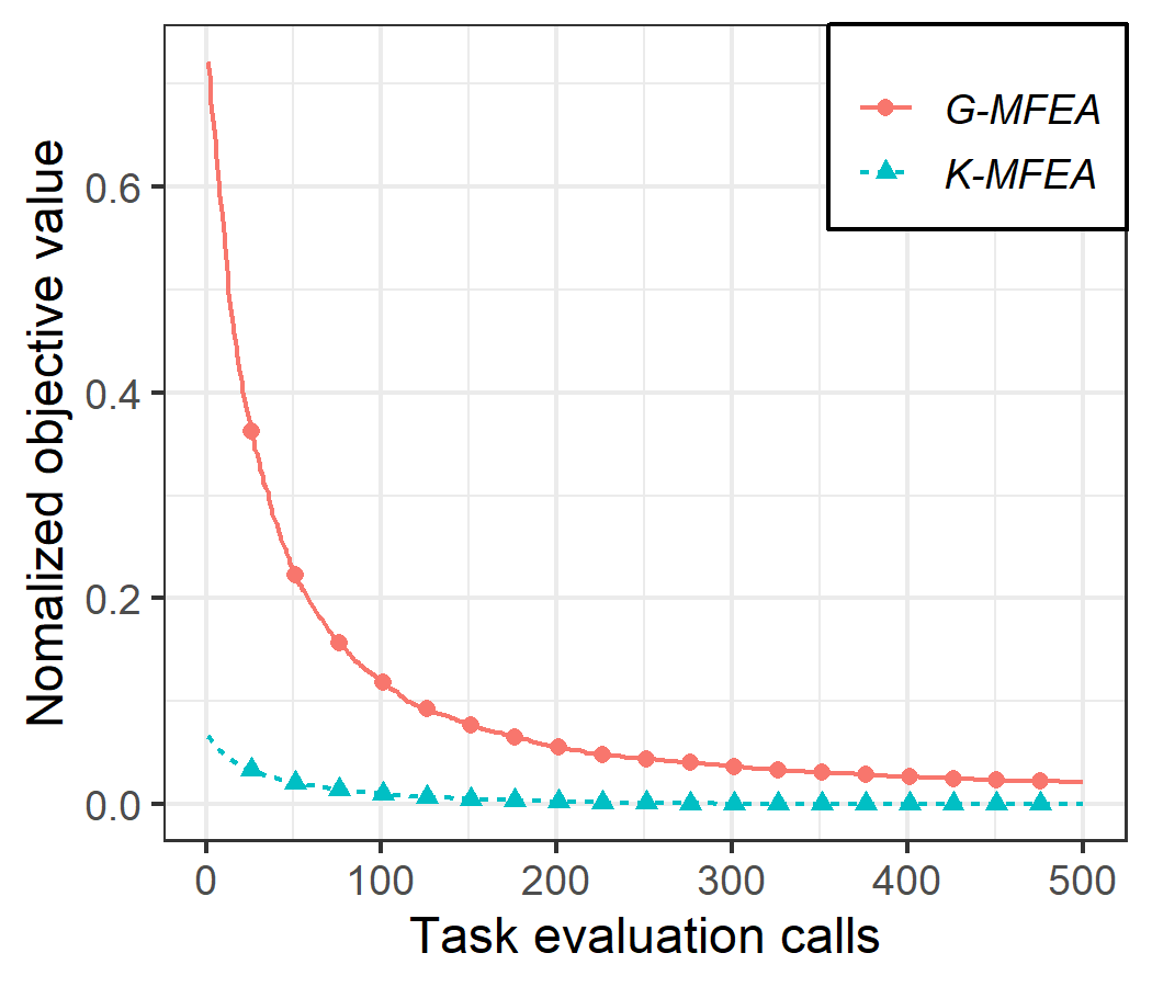
(a) Type 1

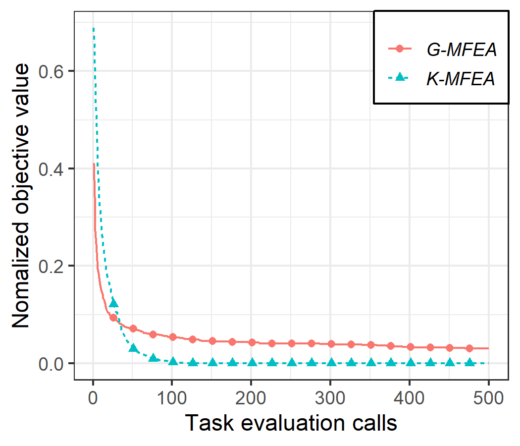
(b) Type 5

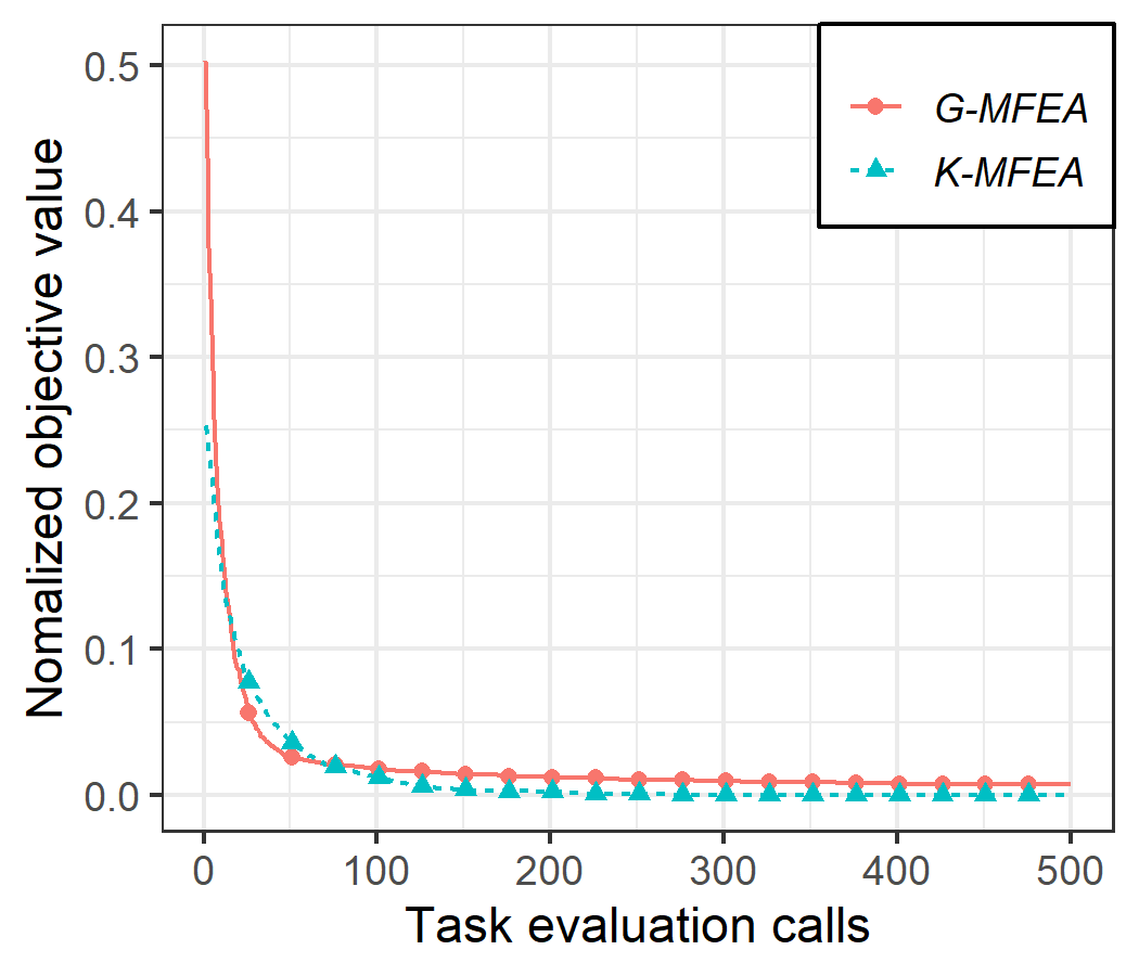
(c) Type 6

Figure 13: Convergence trends of $\tilde{f}$ in multi-tasks and serial single task for instances 10pr439 and 25a280 in Type 1; instances 5i300-108 and 5i400-205 in Type 5; instances 9pcb442-3x3 and 9pr439-3x3 in Type 6.

5.4.5 Analysis influence of the number of parents on results

In this part, we consider the influence of the number of parents of N-MPCX on the performance of K-MFEA. We have conducted experiments in the range of 2 to 10 parents, and the results obtained that are different from running with the two parents are shown in Table 13. In this table, red values indicate better results than values on the left. As shown in the table, the different results are only obtained in large instances and using three or more parents always results in an equal or better experimental result (a better performance is recorded in 12 instances). Besides, the results also show that N-MPCX work most effectively on the parents of 3. The more vertices and clusters a graph has, the better result a multi-parent crossover method brings about. Otherwise, using multiple parents in a smaller set is likely unnecessary because a two-parent crossover operator is sufficient to reach the optimal value. From the above analysis, the N-MPCX is quite suitable in solving large-scale CluSPT problems.

5.4.6 Analysis influence of the speed-up evaluation method

In this part, we compare the performance of the proposed algorithm on aspect running time when it uses and does not use (called K-MFEA ^∗) the speed-up method in subsection 4.8.

Table 8 presents the computational time of algorithms K-MFEA and K-MFEA ^∗ with Min (Max) and Avg are minimum (maximum) and average computational time of algorithms on instances of each type, respectively. Results in this table point out that K-MFEA is faster than K-MFEA ^∗ on all types of instances. On small types, K-MFEA’s average running time is 6.9 to 9.9 times smaller. Whereas on large types, K-MFEA offers 12.8 to 18.8 times less average running time than K-MFEA ^∗. In particular, K-MFEA’s average running time is reduced by 54.7 to 80 times compared to K-MFEA ^∗ on Type 3 and 4 where the average number of vertices per cluster is high. The method in subsection 4.8, thus, has demonstrated its ability to reduce the computational time of the proposed algorithm.

Table 8: Running time of the proposed algorithm when uses and does not use the speed-up evaluation method

	K-MFEA∗			K-MFEA
	Min	Max	Avg	Min	Max	Avg
Type 1 Small	0.167	0.317	0.219	0.001	0.080	0.030
Type 1 Large	0.417	2.067	1.038	0.030	0.150	0.081
Type 3	2.533	2.867	2.720	0.030	0.050	0.034
Type 4	1.267	2.667	1.860	0.030	0.050	0.034
Type 5 Small	0.117	0.300	0.208	0.020	0.030	0.021
Type 5 Large	0.800	2.567	1.409	0.020	0.600	0.075
Type 6 Small	0.117	0.250	0.193	0.020	0.070	0.028
Type 6 Large	0.450	3.650	1.319	0.020	0.470	0.094

6 Conclusion

This paper described a new approach based on MFEA to solve the CluSPT. In the proposed algorithm, the solution encoding method is focused on inter-vertices, while the solution evaluation method uses a mechanism that allows reusing the cost of each cluster to be calculated. Therefore, those help to reduce consuming resources on both computation time and memory space. Furthermore, the crossover, mutation, and decoding operators, as well as a method for repairing invalid individuals, are described to enhance the performance of the proposed MFEA. To evaluate the proposed algorithm, multiple types of Euclidean instances are selected. The results received from the proposed algorithm are state of the art in most test cases in solving CluSPT which strongly proven the efficiency of this approach.

To enhance the performance of the novel algorithm, in the future, the authors will look for evolutionary operators with less complexity.

Table 9: Results obtained by G-MFEA, HB-RGA and K-MFEA on instances in Type 1.

		HB-RGA			G-MFEA			K-MFEA
	Instances	BF	Avg	Time	BF	Avg	Time	BF	Avg	Time
	10berlin52	43738.6	43971	0.04	43724.1	43724.1	0.67	43724.1	43724.1	0.02
	10eil51	1713.2	1723.2	0.04	1713.2	1713.2	0.92	1713.2	1713.2	0.02
	10eil76	2203.3	2208.4	0.05	2203.3	2203.3	1.60	2203.3	2203.3	0.02
	10kroB100	140635.1	141951.4	0.06	140551.2	140597.9	2.35	140522.2	140522.2	0.02
	10pr76	522572.2	525733.1	0.04	522213.8	522340.4	1.67	522213.8	522213.8	0.02
	10rat99	7520.2	7562.1	0.05	7520.2	7524	2.35	7520.2	7520.2	0.02
	10st70	3099.5	3131.7	0.04	3095.2	3095.7	1.40	3095.2	3095.2	0.02
	15berlin52	26312.0	26437.7	0.03	26315.5	26351.7	1.07	26312.0	26312	0.02
	15eil51	1306.7	1313.8	0.03	1306.8	1309.1	1.00	1306.4	1306.4	0.02
	15eil76	2911.3	2921.8	0.04	2909.1	2913.1	1.62	2909.1	2909.1	0.02
	15pr76	705017.3	708944.9	0.04	705226.1	706505.5	1.63	704600.6	704600.6	0.02
	15st70	4129.9	4147.3	0.03	4126.7	4135.5	1.40	4120.1	4120.1	0.02
	25eil101	4680.8	4686.1	0.05	4700.4	4727.9	2.38	4679.0	4679	0.03
	25kroA100	147239.0	147716.8	0.05	148767.9	149708.1	2.37	147195.0	147195	0.03
	25lin105	98087.5	98502.9	0.05	98941.4	100585.3	2.50	97944.7	97944.7	0.03
	25rat99	6846.3	6867.8	0.05	6930.9	7022.3	2.33	6841.5	6841.5	0.03
	50eil101	3827.3	3828.1	0.05	4034.7	4178.1	3.15	3825.3	3825.3	0.08
	50kroA100	159815.2	160029.9	0.05	173113.3	179506.1	3.13	159647.2	159647.2	0.08
	50kroB100	133135.4	133325.8	0.06	149465.6	157831.1	3.13	133104.5	133104.5	0.08
	50lin105	145869.9	145951.8	0.06	151901.5	154680.7	3.33	145829.1	145829.1	0.08
	50rat99	8010.6	8016.8	0.05	8728.0	9002.1	3.15	8007.4	8007.4	0.05
	5berlin52	22746.4	23106.9	0.03	22746.4	22746.4	1.02	22746.4	22746.4	0.05
	5eil51	1770.5	1792.3	0.03	1769.4	1769.4	0.95	1769.4	1769.4	0.00
	5eil76	2630.8	2658.4	0.05	2630.8	2630.8	1.83	2630.8	2630.8	0.00
	5pr76	585008.0	589778.1	0.06	585008.0	585008	1.82	585008.0	585008	0.00
Small instances	5st70	4520.1	4562.8	0.04	4520.1	4520.1	1.57	4520.1	4520.1	0.00
	10a280	28193.6	28515.8	0.31	27936.1	28079.4	14.72	27925.2	27925.2	0.03
	10gil262	27653.6	27788	0.27	27637.5	27645.7	12.78	27637.5	27637.5	0.03
	10lin318	815294.7	825808.2	0.37	812744.1	814264.5	18.55	809750.0	809750	0.03
	10pcb442	745264.4	750362.1	0.87	742112.4	742678.9	39.38	741195.8	741195.8	0.03
	10pr439	1917984.5	1930766.4	1.32	1907568.9	1911815.3	42.50	1904690.2	1904718.9	0.05
	25a280	30058.6	30228.5	0.23	30373.2	30654.1	11.17	29902.4	29902.4	0.05
	25gil262	30535.7	30711.1	0.22	30695.8	30953.2	11.67	30325.7	30325.7	0.07
	25lin318	592166.4	595489	0.31	593017.4	601118.8	16.65	584554.0	584554	0.07
	25pcb442	744734.7	748031.6	0.54	757524.1	762707.5	31.28	740892.6	740892.6	0.07
	25pr439	1519322.1	1531976.6	0.89	1531948.9	1556475.7	29.62	1511168.9	1511197.2	0.07
	50a280	36406.5	36471	0.22	38596.8	39872.5	12.15	36266.9	36266.9	0.13
	50gil262	26634.0	26680.8	0.22	28780.1	30004	12.12	26523.3	26523.3	0.13
	50lin318	690743.8	691897.5	0.31	730023.7	748203.2	16.80	688724.6	688748.6	0.15
	50pcb442	913395.0	914652.8	0.57	962101.7	990436	31.00	910478.7	910487.5	0.15
Large instances	50pr439	2162274.5	2167713.8	0.93	2302262.5	2375177.6	25.13	2152986.6	2152987.9	0.15

Table 10: Results obtained by G-MFEA, HB-RGA and K-MFEA on instances in Types 3 and 4.

		HB-RGA			G-MFEA			K-MFEA
	Instances	BF	Avg	Time	BF	Avg	Time	BF	Avg	Time
	6i300	19461.1	19836.6	0.55	19286.3	19320.3	23.42	19264.5	19264.5	0.03
	6i350	21385.6	21713.4	0.73	21218.5	21261.3	33.20	21217.2	21217.2	0.03
	6i400	29513.4	29913.7	1.05	29389.5	29437.5	46.60	29348.2	29348.2	0.03
	6i450	35899.2	36463.5	1.34	35715.7	35795.9	60.45	35681.5	35681.5	0.03
Type 3	6i500	37799.5	38225.9	1.95	37567.6	37631.4	82.30	37510.1	37516.1	0.05
	4i200a	97959.6	97974.1	0.35	97959.6	97959.6	11.43	97959.6	97959.6	0.02
	4i200h	87675.3	88285.1	0.36	87675.3	87675.3	11.63	87675.3	87675.3	0.02
	4i200x1	123811.4	124825.9	0.35	123669.7	123670.2	11.67	123669.7	123669.7	0.02
	4i200x2	114059.5	115432	0.37	114012.3	114012.3	12.03	114012.3	114012.3	0.02
	4i200z	131807.4	133697.8	0.38	131683.5	131685.2	11.57	131683.5	131683.5	0.02
	4i400a	214115.3	214230.5	2.53	214115.3	214115.3	64.53	214115.3	214115.3	0.02
	4i400h	257054.0	260183.1	2.41	256200.5	256291.2	62.68	256200.5	256200.5	0.03
	4i400x1	188840.1	191145.3	2.32	199389.3	222805.4	36.93	188196.7	188196.7	0.03
	4i400x2	159254.8	162685.6	2.35	176188.2	195580.8	64.03	159254.8	159254.8	0.03
Type 4	4i400z	221460.6	224677.4	2.22	234203.3	244894.6	36.95	221423.9	221423.9	0.03

Table 11: Results obtained by G-MFEA, HB-RGA and K-MFEA on instances in Type 5.

		HB-RGA			G-MFEA			K-MFEA
	Instances	BF	Avg	Time	BF	Avg	Time	BF	Avg	Time
	10i120-46	94055.2	94596.7	0.08	93956.9	94034.3	2.77	93925.0	93925	0.02
	10i30-17	13276.6	13289.2	0.02	13276.6	13276.6	0.58	13276.6	13276.6	0.02
	10i45-18	23267.6	23344.8	0.03	22890.4	22892.2	0.85	22890.4	22890.4	0.02
	10i60-21	33744.5	35002	0.03	33694.8	33702.8	1.20	33694.8	33694.8	0.02
	10i65-21	37386.7	37677	0.04	37353.1	37353.6	1.32	37353.1	37353.1	0.02
	10i70-21	38543.8	38855	0.03	38066.7	38187.3	1.43	38059.5	38059.5	0.02
	10i75-22	65411.9	65783.1	0.05	65362.0	65397.3	1.67	65361.9	65361.9	0.03
	10i90-33	52091.2	52617.6	0.05	51943.2	51975.6	2.03	51931.2	51931.2	0.03
	5i120-46	61776.0	62393.2	0.11	61451.5	61495.3	3.65	61451.5	61451.5	0.02
	5i30-17	14399.9	14399.9	0.02	14399.9	14399.9	0.62	14399.9	14399.9	0.02
	5i45-18	14884.3	14893	0.02	14884.3	14884.3	0.88	14884.3	14884.3	0.02
	5i60-21	28422.7	28584.2	0.03	28422.7	28422.7	1.18	28422.7	28422.7	0.02
	5i65-21	31244.3	31684.7	0.03	30907.8	30911.7	1.40	30907.8	30907.8	0.02
	5i70-21	35052.8	35384.4	0.04	35052.8	35052.8	1.57	35052.8	35052.8	0.02
	5i75-22	34811.1	34993.8	0.05	34692.5	34692.5	1.83	34692.5	34692.5	0.02
	5i90-33	52128.9	52916	0.06	51977.0	51977.3	2.28	51977.0	51977	0.02
	7i30-17	20438.9	20450	0.02	20438.9	20438.9	0.57	20438.9	20438.9	0.02
	7i45-18	20512.0	20973.8	0.02	20512.0	20512	0.80	20512.0	20512	0.02
	7i60-21	36263.9	36339.5	0.03	36263.9	36263.9	1.13	36263.9	36263.9	0.02
Small instances	7i65-21	34847.6	34881.9	0.04	34847.6	34847.6	1.33	34847.6	34847.6	0.02
	10i300-109	113292.8	114274.1	0.33	112876.2	113017.1	16.98	112681.0	112681	0.03
	10i400-206	209409.3	211253.4	0.60	207778.5	208087.4	31.85	207521.7	207521.7	0.03
	10i500-305	352151.4	356961.1	0.99	350897.4	351929.6	52.50	349675.2	349675.2	0.03
	15i300-110	114092.2	114531.8	0.28	112935.9	113358.9	15.83	112096.7	112096.7	0.03
	15i400-207	165565.7	166796.4	0.47	165328.2	165854.9	28.27	164117.8	164117.8	0.03
	15i500-306	305034.5	306929.7	0.80	304128.7	304949.4	42.77	300734.1	300734.1	0.03
	20i300-111	157526.1	158563.7	0.24	157371.4	157990.3	15.30	156347.7	156347.7	0.05
	20i400-208	226173.0	226963.7	0.39	226383.9	227069.5	26.78	224012.5	224012.5	0.05
	20i500-307	203339.4	204679.4	0.64	202938.5	203910.7	39.17	200328.7	200343	0.05
	25i300-112	117661.9	118121.6	0.22	118310.1	119401.3	14.38	116193.6	116193.6	0.05
	25i400-209	231886.7	233015.6	0.38	233552.7	236456.6	23.27	229913.6	229913.6	0.05
	25i500-308	300838.0	301906.8	0.61	302497.1	304046.5	24.60	299498.2	299498.2	0.05
	5i300-108	177698.0	179796.8	0.67	177185.9	177220.7	26.78	177185.9	177185.9	0.02
	5i400-205	210229.5	216014.7	1.17	209488.0	209970.9	52.22	209389.8	209389.8	0.02
Large instances	5i500-304	183130.1	185809.5	2.11	182206.2	182416.4	90.62	182357.0	183976.6	0.60

Table 12: Results obtained by G-MFEA, HB-RGA and K-MFEA on instances in Type 6.

		HB-RGA			G-MFEA			K-MFEA
	Instances	BF	Avg	Time	BF	Avg	Time	BF	Avg	Time
	10berlin52-2x5	27472.4	27723.2	0.04	27471.4	27473	0.83	27471.4	27471.4	0.02
	12eil51-3x4	1699.1	1702.3	0.03	1699.0	1699.1	0.93	1699.0	1699	0.02
	12eil76-3x4	2650.8	2653.2	0.04	2650.8	2650.8	1.57	2650.8	2650.8	0.03
	12pr76-3x4	600597.6	603474.4	0.05	600430.9	600818.7	1.65	600008.6	600008.6	0.03
	12st70-3x4	4128.1	4144.6	0.03	4106.5	4110.1	1.43	4106.5	4106.5	0.03
	15pr76-3x5	526596.7	532896.8	0.06	525170.3	526166.2	1.63	524335.2	524335.2	0.03
	16eil51-4x4	1302.4	1304	0.02	1302.7	1305.6	1.00	1301.4	1301.4	0.03
	16eil76-4x4	2042.4	2053.8	0.04	2040.0	2052.2	1.67	2036.0	2036	0.03
	16lin105-4x4	125052.2	125685.3	0.06	125052.2	125289.8	2.40	125052.2	125052.2	0.03
	16st70-4x4	2939.3	2966.1	0.03	2935.4	2949.2	1.45	2932.6	2932.6	0.03
	18pr76-3x6	642733.0	646399.1	0.04	639723.3	641700.1	1.68	638164.5	638164.5	0.03
	20eil51-4x5	2284.2	2287.9	0.03	2288.7	2295.2	1.05	2283.7	2283.7	0.03
	20eil76-4x5	2385.9	2392.6	0.03	2390.5	2402.2	1.68	2385.9	2385.9	0.03
	20st70-4x5	2939.4	2945.7	0.03	2942.8	2967	1.47	2934.8	2934.8	0.03
	25eil101-5x5	3609.1	3622	0.05	3649.2	3670.5	2.50	3603.5	3603.5	0.03
	25eil51-5x5	1474.6	1476.2	0.02	1487.4	1507.3	1.18	1474.6	1474.6	0.03
	25eil76-5x5	2193.1	2194.8	0.03	2219.1	2245.2	1.73	2193.1	2193.1	0.03
	25rat99-5x5	11400.3	11418.9	0.05	11434.9	11485.9	2.33	11395.8	11395.8	0.03
	28kroA100-4x7	134129.0	134532.3	0.05	136501.1	138342.8	2.38	133101.6	133101.6	0.03
	30kroB100-5x6	198976.7	199205.7	0.05	200596.8	202209.8	2.50	197934.6	197934.6	0.03
	35kroB100-5x5	129122.6	129832.3	0.05	130935.1	132840.4	2.48	129078.7	129078.7	0.03
	36eil101-6x6	3850.7	3852.1	0.04	3929.2	3981.6	2.68	3850.7	3850.7	0.07
	42rat99-6x7	8902.5	8906	0.05	9187.0	9393.5	2.75	8902.1	8902.1	0.07
	4berlin52-2x2	23287.9	23395.9	0.03	23287.9	23287.9	1.10	23287.9	23287.9	0.02
	4eil51-2x2	1898.5	1915.6	0.03	1898.5	1898.5	0.97	1898.5	1898.5	0.02
	4eil76-2x2	2948.8	2974.6	0.05	2948.7	2948.7	1.98	2948.7	2948.7	0.02
	4pr76-2x2	442693.0	445997.3	0.06	442693.0	442693	2.02	442693.0	442693	0.02
	6berlin52-2x3	32130.8	32295.7	0.03	32128.6	32128.6	1.13	32128.6	32128.6	0.02
	6pr76-2x3	648884.9	656228.6	0.05	648275.7	648507.9	1.73	648275.7	648275.7	0.02
	6st70-2x3	3476.7	3503.5	0.04	3476.7	3476.7	1.40	3476.7	3476.7	0.02
	8berlin52-2x4	26854.4	26969.8	0.03	26783.2	26795.4	0.93	26783.2	26783.2	0.02
	9eil101-3x3	3135.4	3154.3	0.06	3117.6	3120.2	2.32	3117.6	3117.6	0.02
	9eil51-3x3	1912.8	1921.3	0.03	1908.0	1909.9	0.92	1907.7	1907.7	0.02
	9eil76-3x3	2938.4	2956.6	0.04	2937.4	2938.6	1.57	2937.4	2937.4	0.02
Small instances	9pr76-3x3	554995.8	560230.3	0.04	553685.6	553849.7	1.63	553400.6	553400.6	0.02
	18pr439-3x6	1475993.8	1498114.4	2.19	1483618.3	1488675.8	57.18	1471788.7	1472798.2	0.07
	20pr439-4x5	1993816.3	2008663.3	1.87	1993350.8	2000099.7	50.65	1978001.3	1978001.3	0.07
	25a280-5x5	42016.8	42150.6	0.24	42123.1	42388.8	13.10	41690.3	41690.3	0.07
	25gil262-5x5	30825.3	31079.8	0.20	31116.2	31372.9	11.60	30649.5	30649.5	0.07
	25pcb442-5x5	748160.1	752959.6	0.59	752573.9	762391.2	28.68	740883.3	740883.3	0.07
	36pcb442-6x6	866373.4	869007.5	0.53	887178.2	901697.8	30.92	860978.2	860993.5	0.10
	42a280-6x7	44080.5	44159.4	0.20	45030.0	46000.9	12.95	43896.8	43896.8	0.10
	49lin318-7x7	572106.1	574040.2	0.28	609127.8	633218.4	15.55	569746.3	569755.3	0.12
	9a280-3x3	29257.3	29497.3	0.36	29045.1	29105	14.55	28947.5	28947.5	0.02
	9gil262-3x3	21248.9	21453.8	0.32	20937.8	20993.1	14.27	20935.9	20935.9	0.02
	9lin318-3x3	720268.4	725327.5	0.47	718479.4	719450.3	20.27	716850.2	716850.2	0.02
	9pcb442-3x3	763118.7	769413.2	1.05	760484.4	761269.1	41.25	760238.3	760238.3	0.02
Large instances	9pr439-3x3	1824280.6	1857520.1	2.86	1803288.2	1809146.2	56.98	1800753.9	1830999.9	0.47

Table 13: The different results obtained by K-MFEA when running with the number of parents in range 2 to 10

Instances		The number of parents
		2	3	4	5
Type 1 large	10pr439	1904718.9	1904690.2	1904690.2	1904690.2
	25pr439	1511197.2	1511168.9	1511168.9	1511168.9
	50lin318	688748.63	688724.60	688724.60	688724.60
	50pcb442	910487.55	910480.10	910478.70	910478.70
	50pr439	2152987.86	2152986.60	2152986.60	2152986.60
Type 3	6i500	37516.12	37,510	37,510	37,510
Type 5 Large	20i500-307	200343	200328.7	200328.7	200328.7
	5i500-304	183976.6	182446	182434.5	182403
Type 6 Large	18pr439-3x6	1472798.2	1471788.7	1471788.7	1471788.7
	9pr439-3x3	1830999.9	1810272.6	1808494.3	1800753.9
	36pcb442-6x6	860993.5	860978.2	860978.2	860978.2
	49lin318-7x7	569755.3	569746.3	569746.3	569746.3

References

- [1] M. D’Emidio, L. Forlizzi, D. Frigioni, S. Leucci, G. Proietti, Hardness, approximability, and fixed-parameter tractability of the clustered shortest-path tree problem, Journal of Combinatorial Optimization 38 (1) (2019) 165–184.
- [2] A. E. Eiben, J. E. Smith, Introduction to evolutionary computing, Springer, 2015.
- [3] P. D. Thanh, H. T. T. Binh, B. T. Lam, New Mechanism of Combination Crossover Operators in Genetic Algorithm for Solving the Traveling Salesman Problem, in: Knowledge and Systems Engineering, Springer, 2015, pp. 367–379.
- [4] T. T. B. Huynh, D. T. Pham, B. T. Tran, C. T. Le, M. H. P. Le, A. Swami, T. L. Bui, A multifactorial optimization paradigm for linkage tree genetic algorithm, Information Sciences 540 (2020) 325–344.
- [5] P. T. H. Hanh, P. D. Thanh, H. T. T. Binh, Evolutionary algorithm and multifactorial evolutionary algorithm on clustered shortest-path tree problem, Information Sciences (2020).
- [6] M. Gong, Z. Tang, H. Li, J. Zhang, Evolutionary multitasking with dynamic resource allocating strategy, IEEE Transactions on Evolutionary Computation 23 (5) (2019) 858–869.
- [7] L. Feng, Y. Huang, L. Zhou, J. Zhong, A. Gupta, K. Tang, K. C. Tan, Explicit evolutionary multitasking for combinatorial optimization: A case study on capacitated vehicle routing problem, IEEE Transactions on Cybernetics (2020).
- [8] L. Zhou, L. Feng, K. C. Tan, J. Zhong, Z. Zhu, K. Liu, C. Chen, Toward adaptive knowledge transfer in multifactorial evolutionary computation, IEEE Transactions on Cybernetics (2020).
- [9] H. T. Binh, P. D. Thanh, T. B. Trung, et al., Effective multifactorial evolutionary algorithm for solving the cluster shortest path tree problem, in: 2018 IEEE Congress on Evolutionary Computation (CEC), IEEE, 2018, pp. 1–8.
- [10] P. D. Thanh, D. A. Dung, T. N. Tien, H. T. T. Binh, An effective representation scheme in multifactorial evolutionary algorithm for solving cluster shortest-path tree problem, in: 2018 IEEE Congress on Evolutionary Computation (CEC), IEEE, 2018, pp. 1–8.
- [11] B. H. T. Thanh, T. P. Dinh, Two levels approach based on multifactorial optimization to solve the clustered shortest path tree problem, Evolutionary Intelligence (2020) 1–29.
- [12] P. D. Thanh, H. T. T. Binh, T. B. Trung, An efficient strategy for using multifactorial optimization to solve the clustered shortest path tree problem, Applied Intelligence 50 (4) (2020) 1233–1258.
- [13] M. Xu, Y. Liu, Q. Huang, Y. Zhang, G. Luan, An improved dijkstra’s shortest path algorithm for sparse network, Applied Mathematics and Computation 185 (1) (2007) 247–254.
- [14] J. A. Chisman, The clustered traveling salesman problem, Computers & Operations Research 2 (2) (1975) 115–119.
- [15] X. Bao, Z. Liu, An improved approximation algorithm for the clustered traveling salesman problem, Information Processing Letters 112 (23) (2012) 908–910.
- [16] K. Helsgaun, Solving the bottleneck traveling salesman problem using the Lin-Kernighan-Helsgaun algorithm, Computer Science Research Report (143) (2011) 1–45.
- [17] A. Gupta, Y.-S. Ong, L. Feng, Multifactorial evolution: toward evolutionary multitasking, IEEE Transactions on Evolutionary Computation 20 (3) (2015) 343–357.
- [18] D. T. Pham, T. T. B. Huynh, An effective combination of genetic algorithms and the variable neighborhood search for solving travelling salesman problem, in: 2015 Conference on Technologies and Applications of Artificial Intelligence (TAAI), IEEE, 2015, pp. 142–149.
- [19] K. K. Bali, Y.-S. Ong, A. Gupta, P. S. Tan, Multifactorial evolutionary algorithm with online transfer parameter estimation: MFEA-II, IEEE Transactions on Evolutionary Computation 24 (1) (2019) 69–83.
- [20] Y.-W. Wen, C.-K. Ting, Parting ways and reallocating resources in evolutionary multitasking, in: 2017 IEEE Congress on Evolutionary Computation (CEC), IEEE, 2017, pp. 2404–2411.
- [21] J. Tang, Y. Chen, Z. Deng, Y. Xiang, C. P. Joy, A group-based approach to improve multifactorial evolutionary algorithm., in: IJCAI, 2018, pp. 3870–3876.
- [22] Y. Yuan, Y.-S. Ong, A. Gupta, P. S. Tan, H. Xu, Evolutionary multitasking in permutation-based combinatorial optimization problems: Realization with tsp, qap, lop, and jsp, in: 2016 IEEE Region 10 Conference (TENCON), IEEE, 2016, pp. 3157–3164.
- [23] H. T. T. Binh, P. D. Thanh, T. B. Thang, New approach to solving the clustered shortest-path tree problem based on reducing the search space of evolutionary algorithm, Knowledge-Based Systems 180 (2019) 12–25.
- [24] M. Mestria, L. S. Ochi, S. de Lima Martins, GRASP with path relinking for the symmetric euclidean clustered traveling salesman problem, Computers & Operations Research 40 (12) (2013) 3218–3229.
- [25] M. D’Emidio, L. Forlizzi, D. Frigioni, S. Leucci, G. Proietti, On the clustered shortest-path tree problem., in: ICTCS, 2016, pp. 263–268.
- [26] P. D. Thanh, CluSPT instances, Mendeley Data v3, 2019. doi:http://dx.doi.org/10.17632/b4gcgybvt6.3.
- [27] P. C. Pop, O. Matei, C. Sabo, A. Petrovan, A two-level solution approach for solving the generalized minimum spanning tree problem, European Journal of Operational Research 265 (2) (2018) 478–487.
- [28] P. D. Thanh, H. T. T. Binh, N. B. Long, A heuristic based on randomized greedy algorithms for the clustered shortest-path tree problem, in: 2019 IEEE Congress on Evolutionary Computation (CEC), IEEE, 2019, pp. 2915–2922.
- [29] J. Derrac, S. García, D. Molina, F. Herrera, A practical tutorial on the use of nonparametric statistical tests as a methodology for comparing evolutionary and swarm intelligence algorithms, Swarm and Evolutionary Computation 1 (1) (2011) 3–18.
- [30] J. Carrasco, S. García, M. M. Rueda, S. Das, F. Herrera, Recent trends in the use of statistical tests for comparing swarm and evolutionary computing algorithms: Practical guidelines and a critical review, Swarm and Evolutionary Computation (2020) 100665.