Using Multiple Pre-treatment Periods to Improve
Difference-in-Differences and Staggered Adoption Designs

Abstract

While a difference-in-differences (DID) design was originally developed with one pre- and one post-treatment period, data from additional pre-treatment periods are often available. How can researchers improve the DID design with such multiple pre-treatment periods under what conditions? We first use potential outcomes to clarify three benefits of multiple pre-treatment periods: (1) assessing the parallel trends assumption, (2) improving estimation accuracy, and (3) allowing for a more flexible parallel trends assumption. We then propose a new estimator, double DID, which combines all the benefits through the generalized method of moments and contains the two-way fixed effects regression as a special case. We show that the double DID requires a weaker assumption about outcome trends and is more efficient than existing DID estimators. We also generalize the double DID to the staggered adoption design where different units can receive the treatment in different time periods. We illustrate the proposed method with two empirical applications, covering both the basic DID and staggered adoption designs. We offer an open-source R package that implements the proposed methodologies.

1 Introduction

Over the last few decades, social scientists have developed and applied various approaches to make credible causal inference from observational data. One of the most popular is a difference-in-differences (DID) design [9, 3]. When the outcome trend of the control group would have been the same as the trend of the outcome in the treatment group in the absence of the treatment (known as the parallel trends assumption), the DID design enables scholars to estimate causal effects even in the presence of time-invariant unmeasured confounding [1]. In its most basic form, we compare treatment and control groups over two time periods — one before and the other after the treatment assignment.

In practice, it is common to apply the DID method with additional pre-treatment periods. However, in contrast to the basic two-time-period case, there are a number of different ways to analyze the DID design with multiple pre-treatment periods. One popular approach is to apply the two-way fixed effects regression to the entire time periods and supplement it with alternative model specifications by including time-trends or leads of the treatment variable to assess possible violations of the parallel trends assumption. Another is to stick with the two-time-period DID and limit the use of additional pre-treatment periods only to the assessment of pre-treatment trends. This variation of approaches raises an important practical question: how should analysts incorporate multiple pre-treatment periods into the DID design, and under what assumptions? In Section 2, we begin by examining three benefits of multiple pre-treatment periods using potential outcomes [24]: (1) assessing the parallel trends assumption, (2) improving estimation accuracy, and (3) allowing for a more flexible parallel trends assumption. While these benefits have been discussed in the literature, we revisit them to clarify that each benefit requires different assumptions and estimators. As a result, in practice, researchers tend to enjoy only a subset of the three benefits they can exploit from multiple pre-treatment periods. While our literature review finds that more than 90% of papers based on the DID design enjoy at least one of the three benefits, we also find that only 20% of the papers enjoy all three benefits.

Our main contribution is to propose a new, simple estimator that achieves all three benefits together. We use the generalized method of moments (GMM) framework [18] to develop the double difference-in-differences (double DID). At its core, we combine two popular DID estimators: the standard DID estimator, which relies on the canonical parallel-trends assumptions, and the sequential DID estimator [28, 32, e.g.,], which only requires that the change in the trends is the same across treatment and control groups (what we call the parallel trends-in-trends assumption). While each estimator itself is not new, the new combination of the two estimators via the GMM allows us to optimally exploit the three benefits of multiple pre-treatment periods.

The proposed double DID approach makes several key methodological contributions. First, we show that the proposed method achieves better theoretical properties than widely-used DID estimators that constitute the double DID. Compared to the standard DID estimator and the two-way fixed effects regression, the double DID has smaller standard errors (i.e., more efficient) and is unbiased under a weaker assumption. While the former estimators require the parallel trends assumption, the double DID only requires the parallel trends-in-trends assumption. The double DID also improves upon the sequential DID estimator, which is inefficient when the parallel trends assumption holds. By using the GMM theory, we show that the double DID is more efficient than the sequential DID when the parallel trends assumption holds. Therefore, our proposed GMM approach enables methodological improvement both in terms of identification and estimation accuracy.

Second, and most importantly in practice, the double DID blends all the three benefits of multiple pre-treatment periods within a single framework. Therefore, instead of using different estimators for enjoying each benefit as required in existing methods, researchers can use the double DID approach to exploit all the benefits. Given that only 20% of papers based on the DID design currently enjoy all the three benefits, our proposed unified approach to optimally exploit all the three benefits of multiple pre-treatment periods is essential in practice.

We also propose three extensions of our double DID estimator. First, we develop the double DID regression, which can incorporate pre-treatment observed covariates to make the DID design more robust and efficient (Section 3.3.1). Second, we allow for any number of pre- and post-treatment periods (Section 3.3.2). While the parallel trends-in-trends assumption can allow for time-varying unmeasured confounders that linearly change over time, we show how to further relax the assumption by accounting for even more flexible forms of time-varying unmeasured confounding when we have more pre-treatment periods. Because our proposed methods allow for any number of post-treatment periods, researchers can also estimate not only short-term causal effects but also longer-term causal effects. Finally, we generalize our double DID estimator to the staggered adoption design where different units can receive the treatment in different time periods (Section 4). This design is increasingly more popular in political science and social sciences [7, 5, 31, e.g.,].

We offer a companion R package DIDdesign that implements the proposed methods. We illustrate our proposed methods through two empirical applications. In Section 3.4, we revisit [30], which study how the abolition of elected councils affects local public services. This serves as an example of the basic DID design where treatment assignment happens only once. In Appendix H.2, we reanalyze [34], which examines the effect of granting collective bargaining rights to teacher’s unions on educational expenditures and teacher’s salaries. This is an example of the staggered adoption design.

Related Literature.

This paper builds on the large literature of time-series cross-sectional data. Generalizing the well-known case of two periods and two groups [1, e.g.,], recent papers use potential outcomes to unpack the nonparametric connection between the DID and two-way fixed effects regression estimators, thereby proposing extensions to relax strong parametric and causal assumptions [36, 23, 11, 5, 16, 22, e.g.,]. Our paper also uses potential outcomes to clarify nonparametric foundations on the use of multiple pre-treatment periods. The key difference is that, while this recent literature mainly considers identification under the parallel trends assumption, we study both estimation accuracy and identification under more flexible assumptions of trends. We do so both in the basic DID setup and in the staggered adoption design.

Another class of popular methods is the synthetic control method [2] and their recent extensions [40, 7, 35, e.g.,] that estimate a weighted average of control units to approximate a treated unit. As carefully noted in those papers, such methodologies require long pre-treatment periods to accurately estimate a pre-treatment trajectory of the treated unit [2]; for example, [40] recommends collecting more than ten pre-treatment periods. In contrast, the proposed double DID can be applied as long as there is more than one pre-treatment period, and is better suited when there are a small to moderate number of pre-treatment periods. However, we also show in Appendix H.2 that the double DID can achieve performance comparable to variants of synthetic control methods even when there are a large number of pre-treatment periods. We offer additional discussions about relationships between our proposed approach and synthetic control methods in Appendix B.

2 Three Benefits of Multiple Pre-treatment Periods

The difference-in-differences (DID) design is one of the most widely used methods to make causal inference from observational studies. The basic DID design consists of treatment and control groups measured at two time periods, before and after the treatment assignment. While the basic DID design only requires data from one post- and one pre-treatment period, additional pre-treatment periods are often available. Unfortunately, however, assumptions behind different uses of multiple pre-treatment periods have often remained unstated.

In this section, we use potential outcomes to discuss three well-known practical benefits of multiple pre-treatment periods: (1) assessing the parallel trends assumption, (2) improving estimation accuracy, and (3) allowing for a more flexible parallel trends assumption. This section serves as a methodological foundation for developing a new approach in Sections 3 and 4.

As our running example, we focus on a study of how the abolition of elected councils affects local public services. [30] use the DID design to examine the effect of recentralization efforts in Vietnam. The abolition of elected councils, the main treatment of interest, was implemented in 2009 in about 12% of all the communes, which are the smallest administrative units that the paper considers. For each commune, a variety of outcomes related to public services, such as the quality of infrastructure, were measured in 2006, 2008, and 2010. With this data, [30] aim to estimate the causal effect of abolishing elected councils on various measures of local public services.

2.1 Setup

To begin with, let $D_{it}$ denote the binary treatment for unit $i$ in time period $t$ so that $D_{it}=1$ if the unit is treated in time period $t$, and $D_{it}=0$ otherwise. In this section, we consider two pre-treatment time periods $t\in\{0,1\}$ and one post-treatment period $t=2$. We choose this setup here because it is sufficient for examining benefits of multiple pre-treatment periods, but we also generalize our methods to an arbitrary number of pre- and post- treatment periods (Section 3.3.2), and to the staggered adoption design (Section 4). In our example, two pre-treatment periods are 2006 and 2008, and one post-treatment period is 2010. Thus, the treatment group receives the treatment only at time $t=2$; $D_{i0}=D_{i1}=0$ and $D_{i2}=1$, whereas units in the control group never gets treated $D_{i0}=D_{i1}=D_{i2}=0$. We refer to the treatment group as $G_{i}=1$ and the control group as $G_{i}=0.$ Outcome $Y_{it}$ is measured at time $t\in\{0,1,2\}.$ In addition to panel data where the same units are measured over time, the DID design accommodates repeated cross-sectional data, in which different communes are sampled at three time periods.

To define causal effects, we rely on the potential outcomes framework [24]. For each time period, $Y_{it}(1)$ represents the quality of infrastructure that commune $i$ would achieve in time period $t$ if commune $i$ had abolished elected councils. $Y_{it}(0)$ is similarly defined. For an individual commune, the causal effect of abolishing elected councils on the quality of infrastructure in time period $t$ is $Y_{it}(1)-Y_{it}(0)$. As the treatment is assigned in the second time period, we are interested in estimating a causal effect at time $t=2$, and a causal effect of interest is formally defined as $Y_{i2}(1)-Y_{i2}(0).$

In the DID design, we are interested in estimating the average treatment effect for treated units (ATT) [3]:

$$\tau=\mathbb{E}[Y_{i2}(1)-Y_{i2}(0)\mid G_{i}=1],$$ (1)

where the expectation is over units in the treatment group $G_{i}=1$.

DID with One Pre-Treatment Period

Before we discuss benefits of multiple pre-treatment periods from Section 2.2, we briefly review the DID with one pre-treatment period to fix ideas for settings with multiple pre-treatment periods.

In the basic DID design, researchers can identify the ATT based on the widely-used assumption of parallel trends — if the treatment group had not received the treatment in the second period, its outcome trend would have been the same as the trend of the outcome in the control group. [3].

Assumption 1 (Parallel Trends).

$$\mathbb{E}[Y_{i2}(0)\mid G_{i}=1]-\mathbb{E}[Y_{i1}(0)\mid G_{i}=1]\ =\ \mathbb{E}[Y_{i2}(0)\mid G_{i}=0]-\mathbb{E}[Y_{i1}(0)\mid G_{i}=0].$$ (2)

The left-hand side of equation (2) is the trend in outcomes for the treatment group $G_{i}=1$, and the right is the one for the control group $G_{i}=0$. Under the parallel trends assumption, we estimate the ATT via the difference-in-differences estimator.

$$\widehat{\tau}_{\texttt{DID}}=\left(\frac{\sum_{i\colon G_{i}=1}Y_{i2}}{n_{12}}-\frac{\sum_{i\colon G_{i}=1}Y_{i1}}{n_{11}}\right)-\left(\frac{\sum_{i\colon G_{i}=0}Y_{i2}}{n_{02}}-\frac{\sum_{i\colon G_{i}=0}Y_{i1}}{n_{01}}\right),$$ (3)

where $n_{1t}$ and $n_{0t}$ are the numbers of units in the treatment and control groups at time $t\in\{1,2\}$, respectively.

When we analyze panel data, we can compute $\widehat{\tau}_{\texttt{DID}}$ nonparametrically via a linear regression with unit and time fixed effects. This numerical equivalence in the two-time-period case is often used to justify the two-way fixed effects regression as the DID design [3]. We discuss additional results on nonparametric equivalence between a regression estimator and the DID estimator in Appendix C.1.

2.2 Benefit 1: Assessing Parallel Trends Assumption

We now consider how researchers can exploit multiple pre-treatment periods, while clarifying necessary underlying assumptions.

The first and the most common use of multiple pre-treatment periods is to assess the identification assumption of parallel trends. As the validity of the DID design rests on this assumption, it is critical to evaluate its plausibility in any application. However, the parallel trends assumption itself involves counterfactual outcomes, and thus analysts cannot empirically test it directly. Instead, we often investigate whether trends for treatment and control groups are parallel in pre-treatment periods as a placebo test [3].

Specifically, researchers often estimate the DID for the pre-treatment periods:

$$\left(\frac{\sum_{i\colon G_{i}=1}Y_{i1}}{n_{11}}-\frac{\sum_{i\colon G_{i}=1}Y_{i0}}{n_{10}}\right)-\left(\frac{\sum_{i\colon G_{i}=0}Y_{i1}}{n_{01}}-\frac{\sum_{i\colon G_{i}=0}Y_{i0}}{n_{00}}\right).$$ (4)

We then check whether the DID estimate on pre-treatment periods is statistically distinguishable from zero. For example, we can apply the DID estimator to 2006 and 2008 as if 2008 were the post-treatment period, and assess whether the estimate would be close to zero. In Figure 1, a DID estimate on the pre-treatment periods would be close to zero for the left panel, while it would be negative for the right panel where two groups have different pre-treatment trends. In Appendix C.4, we show that a robustness check with leads effects [3], which incorporates leads of the treatment variable into the two-way fixed effects regression and checks whether their coefficients are zero, is equivalent to this DID on the pre-treatment periods.

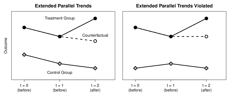
Figure 1: Parallel Pre-treatment Trends (left) and Non-Parallel Pre-treatment Trends (right).

The basic idea behind this test is that if trends are parallel from 2006 to 2008, it is more likely that the parallel trends assumption holds for 2008 and 2010. Hence, instead of considering parallel trends only from 2008 to 2010, the test evaluates the two related parallel trends together. By doing so, this popular test tries to make the DID design falsifiable.

Importantly, this approach does not test the parallel trends assumption itself (Assumption 1), which is untestable due to counterfactual outcomes. Instead, it tests the extended parallel trends assumption — the parallel trends hold for pre-treatment periods, from $t=0$ to $t=1$, as well as from a pre-treatment period $t=1$ to a post-treatment period $t=2$:

Assumption 2 (Extended Parallel Trends).

$$\begin{cases}\mathbb{E}[Y_{i2}(0)\mid G_{i}=1]-\mathbb{E}[Y_{i1}(0)\mid G_{i}=1]=\mathbb{E}[Y_{i2}(0)\mid G_{i}=0]-\mathbb{E}[Y_{i1}(0)\mid G_{i}=0]\\ \mathbb{E}[Y_{i1}(0)\mid G_{i}=1]-\mathbb{E}[Y_{i0}(0)\mid G_{i}=1]=\mathbb{E}[Y_{i1}(0)\mid G_{i}=0]-\mathbb{E}[Y_{i0}(0)\mid G_{i}=0]\end{cases}$$ (5)

The first line of the extended parallel trends assumption is the same as the standard parallel trends assumption, and the second line is the parallel trends for pre-treatment periods. Because outcome trends are observable in pre-treatment periods, the test of pre-treatment trends (equation (4)) directly tests this assumption.

It is important to emphasize that, even if we find the DID estimate on pre-treatment periods is close to zero, we cannot confirm the extended parallel trends assumption (Assumption 2) or the parallel trends assumption (Assumption 1). This is because it is still possible that trends between $t=1$ (pre-treatment) and $t=2$ (post-treatment) are not parallel. Therefore, it is always important to substantively justify the parallel trends assumption in addition to using this statistical test based on pre-treatment trends.

2.3 Benefit 2: Improving Estimation Accuracy

As we discussed above, many existing DID studies that utilize the test of pre-treatment trends can be viewed as the DID design with the extended parallel trends assumption. However, this extended parallel trends assumption is often made implicitly, and thus, it is used only for assessing the parallel trends assumption. Fortunately, if the extended parallel trends assumption holds, we can also estimate the ATT with higher accuracy, resulting in smaller standard errors.

This additional benefit becomes clear by simply restating the extended parallel trends assumption as follows.

$$\begin{cases}\mathbb{E}[Y_{i2}(0)\mid G_{i}=1]-\mathbb{E}[Y_{i1}(0)\mid G_{i}=1]=\mathbb{E}[Y_{i2}(0)\mid G_{i}=0]-\mathbb{E}[Y_{i1}(0)\mid G_{i}=0]\\ \mathbb{E}[Y_{i2}(0)\mid G_{i}=1]-\mathbb{E}[Y_{i0}(0)\mid G_{i}=1]=\mathbb{E}[Y_{i2}(0)\mid G_{i}=0]-\mathbb{E}[Y_{i0}(0)\mid G_{i}=0].\end{cases}$$ (6)

Under the extended parallel trends assumption, there are two natural DID estimators for the ATT.

$$\widehat{\tau}_{\texttt{DID}} =\left(\frac{\sum_{i\colon G_{i}=1}Y_{i2}}{n_{12}}-\frac{\sum_{i\colon G_{i}=1}Y_{i1}}{n_{11}}\right)-\left(\frac{\sum_{i\colon G_{i}=0}Y_{i2}}{n_{02}}-\frac{\sum_{i\colon G_{i}=0}Y_{i1}}{n_{01}}\right),$$

$$\widehat{\tau}_{\texttt{DID(2,0)}} =\left(\frac{\sum_{i\colon G_{i}=1}Y_{i2}}{n_{12}}-\frac{\sum_{i\colon G_{i}=1}Y_{i0}}{n_{10}}\right)-\left(\frac{\sum_{i\colon G_{i}=0}Y_{i2}}{n_{02}}-\frac{\sum_{i\colon G_{i}=0}Y_{i0}}{n_{00}}\right).$$ (7)

Under the extended parallel trends assumption, both estimators are unbiased and consistent for the ATT. Thus, we can increase estimation accuracy by combining the two estimators, for example, simply averaging them.

$$\widehat{\tau}_{\texttt{e-DID}}=\frac{1}{2}\widehat{\tau}_{\texttt{DID}}+\frac{1}{2}\widehat{\tau}_{\texttt{DID(2,0)}}.$$ (8)

Intuitively, this extended DID estimator is more efficient because we have more observations to estimate counterfactual outcomes for the treatment group $\mathbb{E}[Y_{i2}(0)\mid G_{i}=1]$.

In the panel data settings, we show that this extended DID estimator $\widehat{\tau}_{\texttt{e-DID}}$ is equivalent to the two-way fixed effects estimator fitted to the three periods $t\in\{0,1,2\}$.

$$Y_{it}\sim\alpha_{i}+\delta_{t}+\beta D_{it},$$ (9)

where $\alpha_{i}$ is a unit fixed effect, $\delta_{t}$ is a time fixed effect, and a coefficient of the treatment variable $\beta$ is numerically equal to $\widehat{\tau}_{\texttt{e-DID}}$. We also present more general results about nonparametric relationships between the extended DID and the two-way fixed effects estimator in Appendix C.2.

2.4 Benefit 3: Allowing For A More Flexible Parallel Trends Assumption

In this section, we consider scenarios in which the extended parallel trends assumption may not be plausible. Multiple pre-treatment periods are also useful in accounting for some deviation from the parallel trends assumption. We discuss a popular generalization of the difference-in-differences estimator, a sequential DID estimator, which removes bias due to certain violations of the parallel trends assumption [28, 32, e.g.,]. We clarify an assumption behind this simple method and relate it to the parallel trends assumption.

To introduce the sequential DID estimator, we begin with the extended parallel trends assumption. As we described in Section 2.2, when the extended parallel trends assumption holds, a DID estimator applied to pre-treatment periods $t=0$ and $t=1$ should be zero in expectation. In contrast, when trends of treatment and control groups are not parallel, a DID estimate on pre-treatment periods would be non-zero. The sequential DID estimator uses this DID estimate from pre-treatment periods to adjust for bias in the standard DID estimator. In particular, it subtracts the DID estimator on pre-treatment periods from the standard DID estimator that uses pre- and post-treatment periods $t=1$ and $t=2.$

$$\widehat{\tau}_{\texttt{s-DID}} =\left\{\left(\frac{\sum_{i\colon G_{i}=1}Y_{i2}}{n_{12}}-\frac{\sum_{i\colon G_{i}=1}Y_{i1}}{n_{11}}\right)-\left(\frac{\sum_{i\colon G_{i}=0}Y_{i2}}{n_{02}}-\frac{\sum_{i\colon G_{i}=0}Y_{i1}}{n_{01}}\right)\right\}$$

$$\qquad-\left\{\left(\frac{\sum_{i\colon G_{i}=1}Y_{i1}}{n_{11}}-\frac{\sum_{i\colon G_{i}=1}Y_{i0}}{n_{10}}\right)-\left(\frac{\sum_{i\colon G_{i}=0}Y_{i1}}{n_{01}}-\frac{\sum_{i\colon G_{i}=0}Y_{i0}}{n_{00}}\right)\right\},$$ (10)

where the first four terms are equal to the standard DID estimator (equation (3)), and the last four terms are the DID estimator applied to pre-treatment periods $t=0$ and $t=1$ (equation (4)).

This sequential DID estimator requires the parallel trends-in-trends assumption — in the absence of the treatment, the change in the outcome trends of the treatment group is equal to the change in the outcome trends of the control group [32, e.g.,]. While the parallel trends assumption requires that the outcome trends themselves are the same across the treatment and control groups, the parallel trends-in-trends assumption only requires the change in trends over time to be the same. Formally, the parallel trends-in-trends assumption can be written as follows.

Assumption 3 (Parallel Trends-in-Trends).

$$\underbrace{\big{\{}\mathbb{E}[Y_{i2}(0)\mid G_{i}=1]-\mathbb{E}[Y_{i1}(0)\mid G_{i}=1]\big{\}}}_{\text{Trend of the treatment group from $t=1$ to $t=2$}}-\underbrace{\big{\{}\mathbb{E}[Y_{i1}(0)\mid G_{i}=1]-\mathbb{E}[Y_{i0}(0)\mid G_{i}=1]\big{\}}}_{\text{Trend of the treatment group from $t=0$ to $t=1$}}$$ (11)

$$= \underbrace{\big{\{}\mathbb{E}[Y_{i2}(0)\mid G_{i}=0]-\mathbb{E}[Y_{i1}(0)\mid G_{i}=0]\big{\}}}_{\text{Trend of the control group from $t=1$ to $t=2$}}-\underbrace{\big{\{}\mathbb{E}[Y_{i1}(0)\mid G_{i}=0]-\mathbb{E}[Y_{i0}(0)\mid G_{i}=0]\big{\}}}_{\text{Trend of the control group from $t=0$ to $t=1$}}.\hskip 14.45377pt$$

Here, the left-hand side represents how the outcome trends of the treatment group change between (from $t=0$ to $t=1$) and (from $t=1$ to $t=2$). The right-hand side quantifies the same change in the outcome trends for the control group.

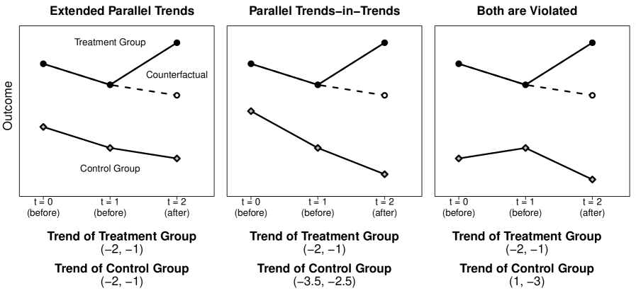
Figure 2: Comparing Extended Parallel Trends and Parallel Trends-in-Trends Assumptions. Note: Below each panel, we report the trends of the control potential outcomes for the treatment and control groups. The first and second elements show the outcome trends (from $t=0$ to $t=1$) and (from $t=1$ to $t=2$), respectively. The extended parallel trends assumption (left panel) means that the outcome trends are the same across the treatment and control groups for both (from $t=0$ to $t=1$) and (from $t=1$ to $t=2$). The parallel trends-in-trends assumption (middle panel) only requires its change over time is the same across the treatment and control groups; $(-1)-(-2)=(-2.5)-(-3.5)=1$. Both assumptions are violated in the right panel.

We also emphasize an alternative way to interpret the parallel trends-in-trends assumption. Unlike the parallel trends assumption that assumes the time-invariant unmeasured confounding, the parallel trends-in-trends assumption can account for linear time-varying unmeasured confounding — unobserved confounding increases or decreases over time but with some constant rate. We provide examples and formal justification of this interpretation in Appendix C.3.3.

Figure 2 visually illustrates that the parallel trends-in-trends assumption holds even when the trends of the treatment and control groups are not parallel, as long as its change over time is the same. Under the parallel trends-in-trends assumption, the sequential DID estimator is unbiased and consistent for the ATT. Importantly, the extended parallel trends assumption is stronger than the parallel trends-in-trends assumption, and thus, the sequential DID estimator is unbiased and consistent for the ATT under the extended parallel trends assumption as well.

We demonstrate that a common robustness check of including group- or unit-specific time trends [3] is nonparametrically equivalent to the sequential DID estimator (see Appendix C.3). Within the potential outcomes framework, we clarified that these common techniques are justified under the parallel trends-in-trends assumption.

3 Double Difference-in-Differences

We saw in the previous section that multiple pre-treatment periods provide the three related benefits. We have clarified that each benefit requires different assumptions and estimators, and as a result, in practice, researchers tend to enjoy only a subset of the three benefits. In this section, we propose a new, simple estimator, which we call the double difference-in-differences (double DID), that blends all the three benefits of multiple pre-treatment periods in a single framework. Here, we introduce the double DID with settings with two pre-treatment periods.

We also provide three extensions. First, we propose the double DID regression to include observed pre-treatment covariates (Section 3.3.1). Second, we generalize the proposed method to any number of pre- and post-treatment periods in the DID design (Section 3.3.2). Finally, we extend it to the staggered adoption design, where the timing of the treatment assignment can vary across units (Section 4).

3.1 Double DID via Generalized Method of Moments

We propose the double DID estimator within a framework of the generalized method of moments (GMM) [18]. In particular, we combine the standard DID estimator and the sequential DID estimator via the GMM:

$$\widehat{\tau}_{\texttt{d-DID}}=\operatornamewithlimits{argmin}_{\tau}\begin{pmatrix}\tau-\widehat{\tau}_{\texttt{DID}}\\[-5.0pt] \tau-\widehat{\tau}_{\texttt{s-DID}}\end{pmatrix}^{\top}\mathbf{W}\begin{pmatrix}\tau-\widehat{\tau}_{\texttt{DID}}\\[-5.0pt] \tau-\widehat{\tau}_{\texttt{s-DID}}\end{pmatrix}\vspace{0.05in}$$ (12)

where $\mathbf{W}$ is a weight matrix of dimension $2\times 2$.

The important property of the proposed double DID estimator is that it contains all of the popular estimators that we considered in the previous sections as special cases. Table 1 illustrates that a particular choice of the weight matrix $\mathbf{W}$ recovers the standard DID, the extended DID, and the sequential DID estimators, respectively.

Using the GMM theory, we can estimate the optimal weight matrix $\widehat{\mathbf{W}}$ such that asymptotic standard errors of the double DID estimator are minimized, which we describe in detail in Section 3.1.2. Therefore, users do not need to manually pick the weight matrix $\mathbf{W}$.

	Standard DID	Extended DID	Sequential DID
Weight Matrix	$\begin{pmatrix}1&0\\ 0&0\end{pmatrix}$	$\begin{pmatrix}3&0\\ 0&-1\end{pmatrix}$	$\begin{pmatrix}0&0\\ 0&1\end{pmatrix}$
$\mathbf{W}$

Table 1: Double DID as Generalization of Popular DID Estimators.

We emphasize that the double DID estimator provides a unifying framework to consider identification assumptions and to estimate treatment effects within the framework of the GMM. The double DID estimator proceeds with the following two steps.

3.1.1 Step 1: Assessing Underlying Assumptions

The first step is to assess the underlying assumptions. We use this first step to adaptively choose the weight matrix $\mathbf{W}$ in the second step. In this first step, we check the extended parallel trends assumption by applying the DID estimator on pre-treatment periods (equation (4)) and testing whether the estimate is statistically distinguishable from zero at a conventional level. To take into account correlated errors, we cluster standard errors at the level of treatment assignment.

Importantly, this step of the double DID can be viewed as the over-identification test in the GMM framework [18], which tests whether all the moment conditions are valid. In the context of the double DID estimator, we assume that the sequential DID estimator is correctly specified and test the null hypothesis that the standard DID estimator is correctly specified. Then, the null hypothesis of the over-identification test becomes exactly the same as testing whether an estimate of the DID estimator applied to pre-treatment periods is equal to zero.

Equivalence Approach. We note that the standard hypothesis testing approach has a risk of conflating evidence for parallel trends and statistical inefficiency. For example, when sample size is small, even if pre-treatment trends of the treatment and control groups differ, a test of the difference might not be statistically significant due to large standard error, and analysts might “pass” the pre-treatment-trends test. To mitigate such concerns, we also incorporate an equivalence approach [19, e.g.,] in which we evaluate the null hypothesis that trends of two groups are not parallel in pre-treatment periods. By using this approach, researchers can “pass” the pre-treatment-trends test only when estimated pre-treatment trends of the two groups are similar with high accuracy, thereby avoiding the aforementioned common mistake. To facilitate the interpretation of the equivalence confidence interval, we report the standardized interval, which can be interpreted as the standard deviation from the baseline control mean. We provide technical details in Appendix F and provide an empirical example in Section 3.4.

3.1.2 Step 2: Estimation of the ATT

The second step is estimation of the ATT. When the extended parallel trends assumption is plausible, we estimate the optimal weight matrix $\widehat{\mathbf{W}}$ building on the theory of the efficient GMM [18]. Specifically, the optimal weight matrix that minimizes the variance of the estimator is given by the inverse of the variance-covariance matrix of the two DID estimators:

$$\widehat{\mathbf{W}}=\begin{pmatrix}\widehat{{\rm Var}}(\widehat{\tau}_{\texttt{DID}})&\widehat{\mbox{Cov}}(\widehat{\tau}_{\texttt{DID}},\widehat{\tau}_{\texttt{s-DID}})\\ \widehat{\mbox{Cov}}(\widehat{\tau}_{\texttt{DID}},\widehat{\tau}_{\texttt{s-DID}})&\widehat{{\rm Var}}(\widehat{\tau}_{\texttt{s-DID}})\end{pmatrix}^{-1}$$ (13)

While the double DID approach can take any weight matrix, this optimal weight matrix allows us to compute the weighted average of the standard DID and the sequential DID estimator such that the resulting variance is the smallest. In particular, when this optimal weight matrix is used, the double DID estimator can be explicitly written as

$$\widehat{\tau}_{\texttt{d-DID}}=w_{1}\widehat{\tau}_{\texttt{DID}}+w_{2}\widehat{\tau}_{\texttt{s-DID}}$$ (14)

where $w_{1}+w_{2}=1$, and

$$w_{1} =\cfrac{\widehat{{\rm Var}}(\widehat{\tau}_{\texttt{s-DID}})-\widehat{\mbox{Cov}}(\widehat{\tau}_{\texttt{DID}},\widehat{\tau}_{\texttt{s-DID}})}{\widehat{{\rm Var}}(\widehat{\tau}_{\texttt{DID}})+\widehat{{\rm Var}}(\widehat{\tau}_{\texttt{s-DID}})-2\widehat{\mbox{Cov}}(\widehat{\tau}_{\texttt{DID}},\widehat{\tau}_{\texttt{s-DID}})},$$

$$w_{2} =\cfrac{\widehat{{\rm Var}}(\widehat{\tau}_{\texttt{DID}})-\widehat{\mbox{Cov}}(\widehat{\tau}_{\texttt{DID}},\widehat{\tau}_{\texttt{s-DID}})}{\widehat{{\rm Var}}(\widehat{\tau}_{\texttt{DID}})+\widehat{{\rm Var}}(\widehat{\tau}_{\texttt{s-DID}})-2\widehat{\mbox{Cov}}(\widehat{\tau}_{\texttt{DID}},\widehat{\tau}_{\texttt{s-DID}})}.$$

By pooling information from both the standard DID and sequential DID, the asymptotic variance of the double DID is smaller than or equal to variance of either the standard and sequential DIDs. This is analogous to Bayesian hierarchical models where pooling information from multiple groups makes estimation more accurate than separate estimation based on each group.

In addition, because the extended DID is a special case of the double DID (as described in Table 1), the asymptotic variance of the double DID is also smaller than or equal to variance of the extended DID. Therefore, ${\rm Var}(\widehat{\tau}_{\texttt{d-DID}})\leq\mbox{min}({\rm Var}(\widehat{\tau}_{\texttt{DID}}),{\rm Var}(\widehat{\tau}_{\texttt{s-DID}}),{\rm Var}(\widehat{\tau}_{\texttt{e-DID}})).$ We provide the proof in Appendix D.

Following [9], we estimate the variance-covariance matrix of $\widehat{\tau}_{\texttt{DID}}$ and $\widehat{\tau}_{\texttt{s-DID}}$ via block-bootstrap where the block is taken at the level of treatment assignment. Specifically, we obtain a pair of two estimators $\{\widehat{\tau}^{(b)}_{\texttt{DID}},\widehat{\tau}^{(b)}_{\texttt{s-DID}}\}$ for $b=1,\ldots,B$ with $B$ number of bootstrap iterations, and compute the empirical variance-covariance matrix. Given an estimate of the weight matrix (equation (13)), we obtain the double DID estimate as a weighted average (equation (14)). We can obtain the variance estimate of $\widehat{\tau}_{\texttt{d-DID}}$ by following the standard efficient GMM variance formula:

$$\widehat{\text{Var}}(\widehat{\tau}_{\texttt{d-DID}})=(\bm{1}^{\top}\widehat{\mathbf{W}}\bm{1})^{-1},$$

where $\bm{1}$ is a two-dimensional vector of ones.

Remark.

Under the extended parallel trends assumption, both the standard DID and the sequential DID estimator are consistent for the ATT, and thus, any weighted average is a consistent estimator. But the optimal weight matrix (equation (13)) chooses the most efficient estimator among all consistent estimators. As we clarify more below, we do not use the weighted average of the standard DID and the sequential DID when the extended parallel trends assumption is violated. ∎

When only the parallel trends-in-trends assumption is plausible, the double DID contains one moment condition $\tau-\widehat{\tau}_{\texttt{s-DID}}=0$, and thus, it reduces to the sequential DID estimator. This is equivalent to choosing the weight matrix $\mathbf{W}$ with $W_{11}=W_{12}=W_{21}=0$ and $W_{22}=1$ (the third column in Table 1).

When both assumptions are implausible, there is no credible estimator for the ATT without making further stringent assumptions. However, when there are more than two pre-treatment periods, researchers can also use the proposed generalized $K$-DID (discussed in Section 3.3.2) to further relax the parallel trends-in-trends assumption.

3.2 Double DID Enjoys Three Benefits

The proposed double DID estimator naturally enjoys the three benefits of multiple pre-treatment periods within a unified framework.

1. Assessing Underlying Assumptions

The double DID incorporates the assessment of underlying assumptions in its first step as the over-identification test. When the trends in pre-treatment periods are not parallel, researchers have to pay the most careful attention to research design and use domain knowledge to assess the parallel trends-in-trends assumption.

2. Improving Estimation Accuracy

When the extended parallel trends assumption holds, researchers can combine two DIDs with equal weights (i.e., the extended DID estimator, which is numerically equivalent to the two-way fixed effects regression) to increase estimation accuracy (Section 2.3). In this setting, the double DID further improves estimation accuracy because it selects the optimal weights as the GMM estimator. In Section G, we use simulations to show that the double DID achieves smaller standard errors than the extended DID estimator.

3. Allowing For A More Flexible Parallel Trends Assumption

Under the parallel trends-in-trends assumption, the double DID estimator converges to the sequential DID estimator. However, when the extended parallel trends assumption holds, the double DID uses optimal weights and is not equal to the sequential DID. Thus, the double DID estimator avoids a dilemma of the sequential DID — it is consistent under a weaker assumption of the parallel trends-in-trends but is less efficient when the extended parallel trends assumption holds. By naturally changing the weight matrix in the GMM framework, the double DID achieves high estimation accuracy under the extended parallel trends assumption and, at the same time, allows for more flexible time-varying unmeasured confounding under the parallel trends-in-trends assumption.

3.3 Extensions

3.3.1 Double DID Regression

Like other DID estimators, the double DID estimator has a nice connection to a regression approach. We propose the double DID regression with which researchers can include other pre-treatment covariates $\mathbf{X}_{it}$ to make the DID design more robust and efficient. We provide technical details in Appendix E.1.

3.3.2 Generalized $K$-Difference-in-Differences

We generalize the proposed method to any number of pre- and post-treatment periods in Appendix E.2, which we call $K$-difference-in-differences ($K$-DID). This generalization has two central benefits. First, it enables researchers to use longer pre-treatment periods to allow for even more flexible forms of unmeasured time-varying confounding beyond the linear time-varying unmeasured confounding under the parallel trends-in-trends assumption (Assumption 3). $K$-DID allows for time-varying unmeasured confounding that follows a $(K-1)$th order polynomial function when researchers have $K$ pre-treatment periods. We can view the double DID as a special case of $K$-DID because in the double DID we have $K=2$ pre-treatment periods, and it can allow for unmeasured confounding that follows ($2-1=1$)st order polynomial function (i.e., a linear function).

Second, we also allow for any number of post-treatment periods so that researchers can estimate not only short-term causal effects but also longer-term causal effects. This generalization can be crucial in many applications because treatment effects might not have an immediate impact on the outcome.

3.4 Empirical Application

[30] utilize the basic DID design to study how the abolition of elected councils affects local public services in Vietnam. To estimate the causal effects of the institutional change, the original authors rely on data from 2008 and 2010, which are before and after the abolition of elected councils in 2009. Then, they supplement the main analysis by assessing trends in pre-treatment periods from 2006 to 2008. In this section, we apply the proposed method and illustrate how to improve this basic DID design.

Although [30] employ the exact same DID design to all of the thirty outcomes they consider, each outcome might require different assumptions, as noted in the original paper. Here, we focus on reanalyzing three outcomes that have different patterns of pre-treatment periods. By doing so, we clarify how researchers can use the double DID method to transparently assess underlying assumptions and employ appropriate DID estimators under different settings. We provide an analysis of all thirty outcomes in Appendix H.1.

3.4.1 Visualizing and Assessing Underlying Assumptions

The first step of the DID design is to visualize trends of treatment and control groups. Figure 3 shows trends of three different outcomes: “Education and Cultural Program,” “Tap Water,” and “Agricultural Center.” Although the original analysis uses the same DID design for all of them, they have distinct trends in the pre-treatment periods. The first outcome of “Education and Cultural Program” has parallel trends in pre-treatment periods. For the other two outcomes, trends do not look parallel in either of the cases. While the trends for the second outcome (“Tap Water”) have similar directions, trends for the third outcome (“Agricultural Center”) have opposite signs. This visualization of trends serves as a transparent first step to assess the underlying assumptions necessary for the DID estimation.

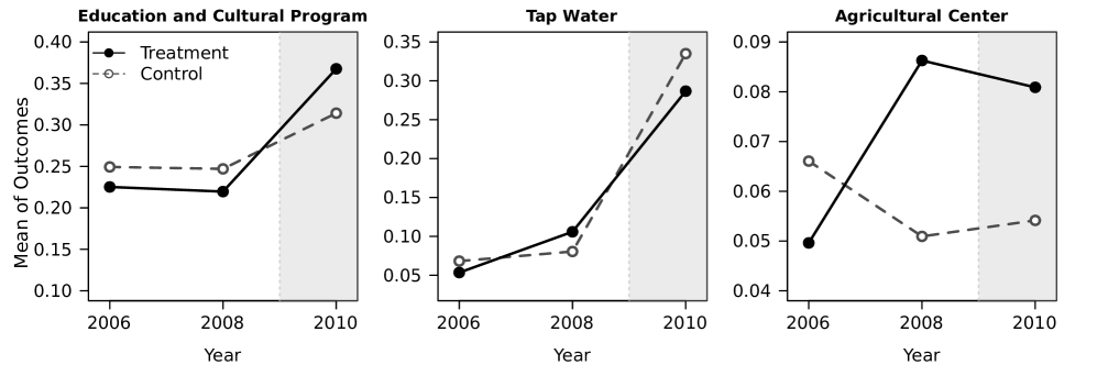
Figure 3: Visualizing Trends of Treatment and Control Groups. Note: We report trends for the treatment group (black solid line with solid circles) and the control group (gray dashed line with hollow circles). Two pre-treatment periods are 2006 and 2008. One post-treatment period, 2010, is indicated by the gray shaded area.

The next step is to formally assess underlying assumptions. As in the original study, it is common to incorporate additional covariates to make the parallel trends assumption more plausible. Based on detailed domain knowledge, [30] include four control variables: area size of each commune, population size, whether national-level city or not, and regional fixed effects. Thus, we assess the conditional extended parallel trends assumption by fitting the DID regression to pre-treatment periods from 2006 to 2008, where $\mathbf{X}_{it}$ includes the four control variables. If the conditional extended parallel trends assumption holds, estimates of the DID regression on pre-treatment trends should be close to zero.

While a traditional approach is to assess whether estimates are statistically distinguishable from zero with the conventional 5% or 10% level, we also report results based on an equivalence approach that we recommend in Section 3. Specifically, we compute the 95% standardized equivalence confidence interval, which quantifies the smallest equivalence range supported by the observed data [19]. In the context of this application, the equivalence confidence interval is standardized based on the mean and standard deviation of the control group in 2006. For example, if the 95% standardized equivalence confidence interval is $[-\nu,\nu],$ this means that the equivalence test rejects the hypothesis that the DID estimate (standardized with respect to the baseline control outcome) on pre-treatment periods is larger than $\nu$ or smaller than $-\nu$ at the 5% level. Thus, the conditional extended parallel trends assumption is more plausible when the equivalence confidence interval is shorter.

The results are summarized in Table 2. Standard errors are computed via block-bootstrap at the district level, where we take 2000 bootstrap iterations. For the first outcome, as the graphical presentation in Figure 3 suggests, a statistical test suggests that the extended parallel trends assumption is plausible.

For the second outcome, the test of the parallel trends reveals that the parallel trends assumption is less plausible for this outcome than for the first outcome. Finally, for the third outcome, both traditional and equivalence approaches provide little evidence for parallel trends, as graphically clear in Figure 3. Although we only have two pre-treatment periods as in the original analysis, if more than two pre-treatment periods are available, researchers can assess the extended parallel trends-in-trends assumption in a similar way by applying the sequential DID estimator to pre-treatment periods. Upon assessing the underlying parallel trends assumptions, we now proceed to estimation of the ATT via the double DID.

	Estimate	Std. Error	p-value	95% Std. Equivalence CI
Education and    Cultural Program	$-0.007$	0.096	0.940	$[-0.166,0.166]$
Tap Water	0.166	0.083	0.045	$[-0.302,0.302]$
Agricultural Center	0.198	0.082	0.015	$[-0.332,0.332]$

Table 2: Assessing Underlying Assumptions Using the Pre-treatment Outcomes. Note: We evaluate the conditional extended parallel trends assumption for three different outcomes. The table reports DID estimates on pre-treatment trends, standard errors, p-values, and the 95% standardized equivalence confidence intervals.

3.4.2 Estimating Causal Effects

Within the double DID framework, we select appropriate DID estimators after the empirical assessment of underlying assumptions. For the first outcome, diagnostics in the previous section suggest that the extended parallel trends assumption is plausible. In such settings, the double DID is expected to produce similar point estimates with smaller standard errors compared to the conventional DID estimator. The first plot of Figure 4 clearly shows this pattern. In the figure, we report point estimates as well as 90% confidence intervals following the original paper (see Figure 3 in [30]). Using the standard DID estimator, the original estimate of the ATT on “Education and Cultural Program” was $0.084$ (90% CI = [$-0.006,0.174$]). Using the double DID estimator, an estimate is instead $0.082$ (90% CI = [$0.001,0.163$]). By using the double DID estimator, we shrink standard errors by about 10%. Although we only have two pre-treatment periods here, when there are more pre-treatment periods, efficiency gain of the double DID can be even larger.

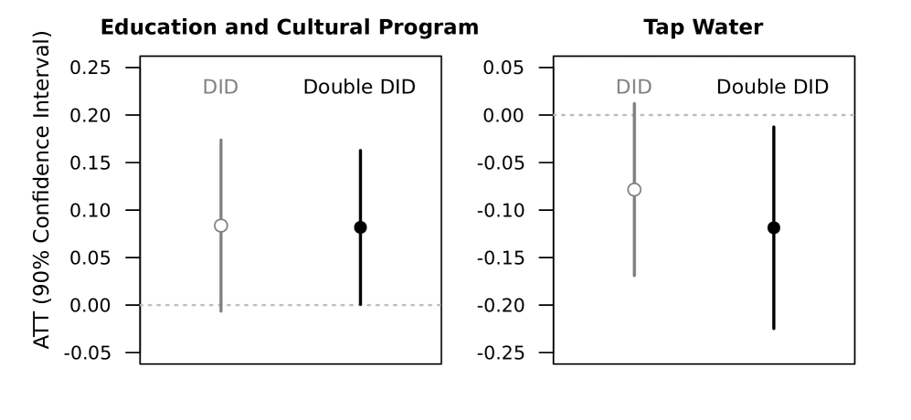
Figure 4: Estimating Causal Effects of Abolishing Elected Councils. Note: We compare estimates from the standard DID and the proposed double DID.

For the second outcome, we did not have enough evidence to support the extended parallel trends assumption. Thus, instead of using the standard DID as in the original analysis, we rely on the parallel trends-in-trends assumption. In this case, the double DID estimates the ATT by allowing for linear time-varying unmeasured confounding in contrast to the standard DID that assumes constant unmeasured confounders. The second plot of Figure 4 shows the important difference between the two methods. While the standard DID estimates is $-0.078$ (90% CI = [$-0.169,0.012$]), the double DID estimate is $-0.119$ (90% CI = [$-0.225,-0.012$]). Given that the extended parallel trends assumption is not plausible, this result suggests that the standard DID suffers from substantial bias (the bias of $0.04$ corresponds to more than 50% of the original point estimate). By incorporating non-parallel pre-treatment trends, the double DID shows that the original DID estimate was underestimated by a large amount.

Finally, for the third outcome, the previous diagnostics suggest that the extended parallel trends assumption is implausible. It is possible to use the double DID under the parallel trends-in-trends assumption. However, trends of treatment and control groups have opposite signs, implying the double DID estimates are highly sensitive to the parallel trends-in-trends assumption. Given that the parallel trends-in-trends assumption is also difficult to justify here, there is no credible estimator of the ATT without making additional stringent assumptions. While we focused on the three outcomes here, the double DID improves upon the standard DID in a similar way for the other outcomes as well (see Appendix H.1).

4 Staggered Adoption Design

In this section, we extend the proposed double DID estimator to the staggered adoption design where the timing of the treatment assignment can vary across units [36, 7, 5].

4.1 The Setup and Causal Quantities of Interest

In the staggered adoption (SA) design, different units can receive the treatment in different time periods. Once they receive the treatment, they remain exposed to the treatment afterward. Therefore, $D_{it}=1$ if $D_{im}=1$ where $m<t.$ We can thus summarize information about the treatment assignment by the timing of the treatment $A_{i}$ where $A_{i}\equiv\mbox{min}\ \{t:D_{it}=1\}.$ When unit $i$ never receives the treatment until the end of time $T$, we let $A_{i}=\infty.$ For example, in many applications where researchers are interested in the causal effect of state- or local-level policies, units adopt policies in different time points and remain exposed to such policies once they introduce the policies. In Appendix H.2, we provide its example based on [34]. See Figure 5 for visualization of the SA design.

Following the recent literature on the SA design, we make two standard assumptions in the SA design: no anticipation assumption and invariance to history assumption [23, 5]. This implies that, for unit $i$ in period $t$, the potential outcome $Y_{it}(1)$ represents the outcome of unit $i$ that would realize in period $t$ if unit $i$ receives the treatment at or before period $t$. Similarly, $Y_{it}(0)$ represents the outcome of unit $i$ that would realize in period $t$ if unit $i$ does not receive the treatment by period $t$. Finally, we generalize group indicator $G$ as follows.

$$G_{it}\ =\ \begin{cases}\ \ 1&\mbox{if }A_{i}=t\\ \ \ 0&\mbox{if }A_{i}>t\\ \ \ -1&\mbox{if }A_{i}<t\end{cases}$$ (15)

where $G_{it}=1$ represents units who receive the treatment at time $t$, and $G_{it}=0$ ($G_{it}=-1$) indicates units who receive the treatment after (before) time $t$.

Under the SA design, the staggered adoption ATT (SA-ATT) at time $t$ is defined as follows.

$$\tau^{\textsf{SA}}(t)=\mathbb{E}[Y_{it}(1)-Y_{it}(0)\mid G_{it}=1],$$

which represents the causal effect of the treatment in period $t$ on units with $G_{it}=1$, who receive the treatment at time $t.$ This is a straightforward extension of the standard ATT (equation (1)) in the basic DID setting. Researchers might also be interested in the time-average staggered adoption ATT (time-average SA-ATT).

$$\overline{\tau}^{\textsf{SA}}=\sum_{t\in\mathcal{T}}\pi_{t}\tau^{\textsf{SA}}(t),$$

where $\mathcal{T}$ represents a set of the time periods for which researchers want to estimate the ATT. For example, if a researcher is interested in estimating the ATT for the entire sample periods, one can take $\mathcal{T}=\{1,\ldots,T\}$. The SA-ATT in period $t$, $\tau^{\textsf{SA}}(t),$ is weighted by the proportion of units who receive the treatment at time $t$: $\pi_{t}=\sum_{i=1}^{n}\mathbf{1}\{A_{i}=t\}/\sum_{i=1}^{n}\mathbf{1}\{A_{i}\in\mathcal{T}\}$.

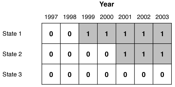
Figure 5: Example of the Staggered Adoption Design. Note: We use gray cells of “1” to denote the treated observation and use white cells of “0” to denote the control observation.

4.2 Double DID for Staggered Adoption Design

Under what assumptions can we identify the SA-ATT and the time-average SA-ATT? Here, we first extend the standard DID estimator under the parallel trends assumption and the sequential DID estimator under the parallel trends-in-trends assumption to the SA design. Formally, we define the standard DID estimator for the SA-ATT at time $t$ as

$$\widehat{\tau}^{\textsf{SA}}_{\texttt{DID}}(t)=\left(\frac{\sum_{i\colon G_{it}=1}Y_{it}}{n_{1t}}-\frac{\sum_{i\colon G_{it}=1}Y_{i,t-1}}{n_{1,t-1}}\right)-\left(\frac{\sum_{i\colon G_{it}=0}Y_{it}}{n_{0t}}-\frac{\sum_{i\colon G_{it}=0}Y_{i,t-1}}{n_{0,t-1}}\right),\vspace{10pt}$$

which is consistent for the SA-ATT under the following parallel trends assumption in period $t$ under the SA design:

$$\mathbb{E}[Y_{it}(0)\mid G_{it}=1]-\mathbb{E}[Y_{i,t-1}(0)\mid G_{it}=1]\ =\ \mathbb{E}[Y_{it}(0)\mid G_{it}=0]-\mathbb{E}[Y_{i,t-1}(0)\mid G_{it}=0].$$

Similarly, we can define the sequential DID estimator for the SA-ATT at time $t$ as

$$\widehat{\tau}^{\textsf{SA}}_{\texttt{s-DID}}(t) =\left\{\left(\frac{\sum_{i\colon G_{it}=1}Y_{it}}{n_{1t}}-\frac{\sum_{i\colon G_{it}=1}Y_{i,t-1}}{n_{1,t-1}}\right)-\left(\frac{\sum_{i\colon G_{it}=0}Y_{it}}{n_{0t}}-\frac{\sum_{i\colon G_{it}=0}Y_{i,t-1}}{n_{0,t-1}}\right)\right\}$$

$$\qquad-\left\{\left(\frac{\sum_{i\colon G_{it}=1}Y_{i,t-1}}{n_{1,t-1}}-\frac{\sum_{i\colon G_{it}=1}Y_{i,t-2}}{n_{1,t-2}}\right)-\left(\frac{\sum_{i\colon G_{it}=0}Y_{i,t-1}}{n_{0,t-1}}-\frac{\sum_{i\colon G_{it}=0}Y_{i,t-2}}{n_{0,t-2}}\right)\right\},$$

which is consistent for the SA-ATT under the following parallel trends-in-trends assumption in period $t$ under the SA design:

$$\{\mathbb{E}[Y_{it}(0)\mid G_{it}=1]-\mathbb{E}[Y_{it}(0)\mid G_{it}=0]\}-\{\mathbb{E}[Y_{i,t-1}(0)\mid G_{it}=1]-\mathbb{E}[Y_{i,t-1}(0)\mid G_{it}=0]\}$$

$$=\{\mathbb{E}[Y_{i,t-1}(0)\mid G_{it}=1]-\mathbb{E}[Y_{i,t-1}(0)\mid G_{it}=0]\}-\{\mathbb{E}[Y_{i,t-2}(0)\mid G_{it}=1]-\mathbb{E}[Y_{i,t-2}(0)\mid G_{it}=0]\}.$$

Finally, combining the standard and sequential DID estimators, we can extend the double DID to the SA design as follows.

$$\widehat{\tau}^{\textsf{SA}}_{\texttt{d-DID}}(t)=\operatornamewithlimits{argmin}_{\tau^{\textsf{SA}}(t)}\begin{pmatrix}\tau^{\textsf{SA}}(t)-\widehat{\tau}^{\textsf{SA}}_{\texttt{DID}}(t)\\[-5.0pt] \tau^{\textsf{SA}}(t)-\widehat{\tau}^{\textsf{SA}}_{\texttt{s-DID}}(t)\end{pmatrix}^{\top}\mathbf{W}(t)\begin{pmatrix}\tau^{\textsf{SA}}(t)-\widehat{\tau}^{\textsf{SA}}_{\texttt{DID}}(t)\\[-5.0pt] \tau^{\textsf{SA}}(t)-\widehat{\tau}^{\textsf{SA}}_{\texttt{s-DID}}(t)\end{pmatrix}\vspace{0.05in}$$

where $\mathbf{W}(t)$ is a weight matrix. Under the SA design, similar to the basic design, the standard DID and sequential DID estimators are special cases of our proposed double DID estimator with specific choices of the weight matrix. As in Section 3.1, we can estimate the optimal weight matrix $\widehat{\mathbf{W}}(t)$ (details below), and thus, users do not need to choose it manually.

Like the basic double DID estimator in Section 3.1, the double DID for the SA design also consists of two steps. The first step is to assess the underlying assumptions using the standard DID for the SA design with two points $\{t-1,t-2\}$ for units that are not yet treated at time $t-1$, that is, $\{i:G_{it}\geq 0\}$. This is a generalization of the pre-treatment-trends test in the basic DID setup (Section 2.2). The second step is to estimate the SA-ATT at time $t$. When only the parallel trends-in-trends assumption is plausible, we choose weight matrix $\mathbf{W}(t)$ where $\mathbf{W}(t)_{11}=\mathbf{W}(t)_{12}=\mathbf{W}(t)_{21}=0$ and $\mathbf{W}(t)_{22}=1$, which converges to the sequential DID under the SA design. When the extended parallel trends assumption is plausible, we use the optimal weight matrix defined as $\widehat{\mathbf{W}}(t)=\widehat{{\rm Var}}(\widehat{\tau}^{\textsf{SA}}_{(1:2)}(t))^{-1}$ where ${\rm Var}(\cdot)$ is the variance-covariance matrix and $\widehat{\tau}^{\textsf{SA}}_{(1:2)}(t)=(\widehat{\tau}^{\textsf{SA}}_{\texttt{DID}}(t),\widehat{\tau}^{\textsf{SA}}_{\texttt{s-DID}}(t))^{\top}.$ This optimal weight matrix provides us with the most efficient estimator (i.e., the smallest standard error). We provide further details on the implementation in Appendix E.3.

To estimate the time-average SA-DID, we extend the double DID as follows.

$$\widehat{\overline{\tau}}^{\textsf{SA}}_{\texttt{d-DID}}=\operatornamewithlimits{argmin}_{\overline{\tau}^{\textsf{SA}}}\begin{pmatrix}\overline{\tau}^{\textsf{SA}}-\widehat{\overline{\tau}}^{\textsf{SA}}_{\texttt{DID}}\\[-5.0pt] \overline{\tau}^{\textsf{SA}}-\widehat{\overline{\tau}}^{\textsf{SA}}_{\texttt{s-DID}}\end{pmatrix}^{\top}\overline{\mathbf{W}}\begin{pmatrix}\overline{\tau}^{\textsf{SA}}-\widehat{\overline{\tau}}^{\textsf{SA}}_{\texttt{DID}}\\[-5.0pt] \overline{\tau}^{\textsf{SA}}-\widehat{\overline{\tau}}^{\textsf{SA}}_{\texttt{s-DID}}\end{pmatrix}\vspace{0.05in}$$

where $\widehat{\overline{\tau}}^{\textsf{SA}}_{\texttt{DID}}$ and $\widehat{\overline{\tau}}^{\textsf{SA}}_{\texttt{s-DID}}$ are time-averages of the DID and sequential DID estimators,

$$\widehat{\overline{\tau}}^{\textsf{SA}}_{\texttt{DID}}=\sum_{t\in\mathcal{T}}\pi_{t}\widehat{\tau}^{\textsf{SA}}_{\texttt{DID}}(t),\hskip 14.45377pt\mbox{and}\hskip 14.45377pt\widehat{\overline{\tau}}^{\textsf{SA}}_{\texttt{s-DID}}=\sum_{t\in\mathcal{T}}\pi_{t}\widehat{\tau}^{\textsf{SA}}_{\texttt{s-DID}}(t).$$

The optimal weight matrix $\widehat{\overline{\mathbf{W}}}$ is equal to $\widehat{{\rm Var}}(\widehat{\overline{\tau}}^{\textsf{SA}}_{(1:2)})^{-1}$ where $\widehat{\overline{\tau}}^{\textsf{SA}}_{(1:2)}=(\widehat{\overline{\tau}}^{\textsf{SA}}_{\texttt{DID}},\widehat{\overline{\tau}}^{\textsf{SA}}_{\texttt{s-DID}})^{\top}.$

5 Concluding Remarks

While the most basic form of the DID only requires two time periods — one before and the other after treatment assignment, researchers can often collect data from several additional pre-treatment periods in a wide range of applications. In this article, we show that such multiple pre-treatment periods can help improve the basic DID design and the staggered adoption design in three ways: (1) assessing underlying assumptions about parallel trends, (2) improving estimation accuracy, and (3) enabling more flexible DID estimators. We use the potential outcomes framework to clarify assumptions required to enjoy each benefit.

We then propose a simple method, the double DID, to combine all three benefits within the GMM framework. Importantly, the double DID contains the popular two-way fixed effects regression and nonparametric DID estimators as special cases, and it uses the GMM to further improve with respect to identification and estimation accuracy. Finally, we generalize the double DID estimator to the staggered adoption design where the timing of the treatment assignment can vary across units.

References.1References.1ReferencesReferencesReferences.1

Appendix A Literature Review

A.1 Papers in APSR and AJPS

We conduct a review of the literature to assess current practices of the difference-in-differences (DID) design. Specifically, we search articles published in American Political Science Review and American Journal of Political Science from 2015 to 2019. Some of the papers we reviewed were accepted in 2019 and were officially published in 2020. Using Google Scholar, we find articles that contains any of the following keywords: “two-way fixed effect”, “two-way fixed effects”, “difference in difference” or “difference in differences.” We then manually select articles from the list that uses the basic DID design and the staggered adoption design (see the main text for details about the first two design). This procedure left us with a total of 25 articles, 11 from APSR and 14 from AJPS. Table A1 and A2 show the articles in the list published in APSR and AJPS, respectively.

To determine the number of pre-treatment periods, we manually assess the listed articles. Among the 25 articles, 20 articles use the basic DID design, and 5 articles use the staggered adoption design. When a paper uses the basic DID design, we can determine the length of the pre-treatment periods from the data description and the time of the treatment assignment. On the other hand, the pre-treatment periods for the staggered adoption and the general design are set to the total number of time-periods available in the data, as the length of pre-treatment periods varies across units.

We found that most DID applications have less than 10 pre-treatment periods. The median number of pre-treatment periods is $3.5$ and, the mean number of pre-treatment periods is about $6$ after removing one unique study that has more than $100$ pre-treatment periods.

A.2 Examples of Two Common Approaches

As we wrote in Section 1, there are several different popular ways to analyze the DID design with multiple pre-treatment periods. One common approach is to apply the two-way fixed effects regression to the entire time periods, and supplement it with alternative model specifications by including time-trends or leads of the treatment variable to assess possible violations of the parallel trends assumption. Examples include [13, 38, 14, 17, 27]. Another is to stick with the two-time-period DID and limit the use of additional pre-treatment periods only to the assessment of pre-treatment trends. Examples include [26, 6, 10, 25, 15]. Note that we list exemplary papers here and thus, we also include papers from journals other than APSR and AJPS.

Table A1: DID papers on APSR.

Authors	Year	Title
O’brien, D. Z., & Rickne J.	2016	Gender Quotas And Women’s Political Leadership
Garfias, F.	2018	Elite Competition and State Capacity Development: Theory and Evidence From Post-Revolutionary Mexico.
Martin, G. J., & Mccrain, J.	2019	Local News And National Politics
Blom-Hansen, J., Houlberg, K.,    Serritzlew, S., & Treisman, D.	2016	Jurisdiction Size and Local Government Policy Expenditure: Assessing The Effect of Municipal Amalgamation
Clinton, J. D., & Sances, M. W.	2018	The Politics of Policy: The Initial Mass Political Effects of Medicaid Expansion in The States
Malesky, E. J. , Nguyen, C. V.,    & Tran, A.	2014	The Impact of Recentralization on Public Services: A Difference-in-Differences Analysis of the Abolition of Elected Councils in Vietnam.
Larsen, M. V., Hjorth, F.,    Dinesen, P. T.,    & Sønderskov, K. M.	2019	When Do Citizens Respond Politically to The Local Economy? Evidence From Registry Data on Local Housing Markets
Becher, M., & González, I. M.	2019	Electoral Reform and Trade-Offs in Representation
Selb, P., & Munzert, S.	2018	Examining A Most Likely Case for Strong Campaign Effects
Enos, R. D., Kaufman, A. R.,    & Sands, M. L.	2019	Can Violent Protest Change Local Policy Support?
Vasiliki Fouka	2019	How Do Immigrants Respond to Discrimination?

Table A2: DID papers on AJPS.

Authors	Year	Title
Bechtel, M. M., Hangartner, D.,    & Schmid, L.	2016	Does compulsory voting increase support for leftist policy?
Bisgaard, M., & Slothuus, R.	2018	Partisan elites as culprits? How party cues shape partisan perceptual gaps.
Bischof, D., & Wagner, M.	2019	Do voters polarize when radical parties enter parliament?
Dewan, T., Meriläinen, J.,    & Tukiainen, J.	2020	Victorian voting: The origins of party orientation and class alignment.
Earle, J. S., & Gehlbach, S.	2015	The Productivity Consequences of Political Turnover: Firm-Level Evidence from Ukraine’s Orange Revolution.
Enos, R. D.	2016	What the demolition of public housing teaches us about the impact of racial threat on political behavior.
Gingerich, D. W.	2019	Ballot Reform as Suffrage Restriction: Evidence from Brazil’s Second Republic.
Hainmueller, J, & Hangartner, D.	2019	Does direct democracy hurt immigrant minorities? Evidence from naturalization decisions in Switzerland.
Holbein, J. B., & Hillygus, D. S.	2016	Making young voters: the impact of preregistration on youth turnout.
Jäger, K.	2020	When Do Campaign Effects Persist for Years? Evidence from a Natural Experiment.
Lindgren, K. O., Oskarsson, S.,    & Dawes, C. T.	2017	Can Political Inequalities Be Educated Away? Evidence from a Large-Scale Reform.
Lopes da Fonseca, M.	2017	Identifying the source of incumbency advantage through a constitutional reform.
Paglayan, AS.	2019	Public-Sector Unions and the Size of Government
Pardos-Prado, S., & Xena, C.	2019	Skill specificity and attitudes toward immigration.

Appendix B Comparison with Three Existing Methods

This section clarifies relationships between our proposed double DID and three existing methods: the two-way fixed effects estimator, the sequential DID estimator, and synthetic control methods.

B.1 Relationship with Two-Way Fixed Effects Estimator

While we contrast the double DID with the two-way fixed effects estimator throughout the paper, we summarize our discussion here. First, in the basic DID design, the two-way fixed effects estimator is a special case of the double DID with a specific choice of the weight matrix $\mathbf{W}$ (see Table 1). Therefore, whenever the two-way fixed effects estimator is consistent for the ATT, the double DID is a more efficient, consistent estimator of the ATT. This is because the double DID can choose the optimal weight matrix via the GMM, while the two-way fixed effects uses the pre-determined equal weights over time. Second, in the SA design, a large number of recent papers show that the widely-used two-way fixed effects estimator are in general inconsistent for the ATT due to treatment effect heterogeneity and implicit parametric assumptions [36, 5, 22, 37]. In contrast, the proposed double DID in the SA design generalizes nonparametric DID estimators to allow for treatment effect heterogeneity, and thus, it does not suffer from the same problem.

B.2 Relationship with Sequential DID Estimator

Our double DID estimator contains the sequential DID estimator [28, 32, e.g.,] as a special case. Our proposed double DID improves over the sequential DID estimator in two ways. First, when the parallel trends assumption holds, the double DID optimally combine the standard DID and the sequential DID to improve efficiency, and it is not equal to the sequential DID. Therefore, it avoids a dilemma of the sequential DID — it is consistent under the parallel trends-in-trends assumption (weaker than the parallel trends assumption), but is less efficient when the parallel trends assumption holds. Second, while the sequential DID estimator has only been available for the basic DID design where treatment assignment happens only once, we generalize it to the staggered adoption design and further incorporate it into our staggered-adoption double DID estimator (Section 4).

B.3 Relationship with Synthetic Control Methods

Another relevant popular class of methods is the synthetic control methods. While the method was originally designed to estimate the causal effect on a single treated unit, recent extensions allow for multiple treated units and the staggered adoption design [40, 8, 20, 4, e.g.,]. Despite a wide variety of innovative extensions, they all share the same core feature: they require long pre-treatment periods to accurately estimate a pre-treatment trajectory of the treated units. For example, [40] recommends collecting more than ten pre-treatment periods. In contrast, the proposed double DID can be applied as long as there are more than one pre-treatment periods, and is better suited when there are a small to moderate number of pre-treatment periods.

When there are a large number of pre-treatment periods (i.e., long enough to apply the synthetic control methods), we recommend to apply both the synthetic control methods and proposed double DID, and evaluate robustness across those approaches. This is important because they rely on different identification assumptions. In fact, we show in Section H.2, the double DID can recover credible estimates similar to more flexible variants of synthetic control methods even when there are a large number of pre-treatment periods. This robustness provides researchers with additional credibility for their causal estimates and underlying assumptions.

Appendix C Nonparametric Equivalence to Regression Estimators

In this section, we provide results on the nonparametric connection between regression estimators and the three DID estimators we discussed in the paper. This section provides methodological foundations for our main methodological contributions, which we prove in Sections E.2 and E.3.

C.1 Standard DID

In practice, we can compute the DID estimator via a linear regression. We regress the outcome $Y_{it}$ on an intercept, treatment group indicator $G_{i}$, time indicator $I_{t}$ (equal to $1$ if post-treatment and $0$ otherwise) and the interaction between the treatment group indicator and the time indicator $G_{i}\times I_{t}$.

$$Y_{it}\sim\alpha+\theta G_{i}+\gamma I_{t}+\beta(G_{i}\times I_{t}),$$ (A.2)

where $(\alpha,\theta,\gamma,\beta)$ are corresponding coefficients. In this case, a coefficient of the interaction term $\beta$ is numerically equal to the DID estimator, $\widehat{\tau}_{\texttt{DID}}$. Importantly, the linear regression is used here only to compute the nonparametric DID estimator (equation (3)), and thus it does not require any parametric modeling assumption such as constant treatment effects. Furthermore, when we analyze panel data in which the same units are observed repeatedly over time, we obtain exactly the same estimate via a linear regression with unit and time fixed effects. This numerical equivalence in the two-time-period case is often the justification of the two-way fixed effects regression as the DID design [3]. The above equivalence is formally shown below for completeness.

C.1.1 Repeated Cross-Sectional Data

For the later use in this Appendix, we report the well-known result that the standard DID estimator $\widehat{\tau}_{\texttt{DID}}$ (equation (3)) is equivalent to coefficient $\widehat{\beta}$ in the regression estimator (equation (A.2)) [1].

We define $O_{it}$ to be an indicator variable taking the value $1$ when individual $i$ is observed in time period $t$. Using this notation, we prove the following result.

Result 1 (Nonparametric Equivalence of the Standard DID and Regression Estimator).

We write the linear regression estimator (equation (A.2)) as a solution to the following least squares problem.

$$(\widehat{\alpha},\widehat{\theta},\widehat{\gamma},\widehat{\beta})=\operatornamewithlimits{argmin}\sum^{n}_{i=1}\sum_{t=1}^{2}O_{it}\Big{\{}Y_{it}-\alpha-\theta G_{i}-\gamma I_{t}-\beta(G_{i}\times I_{t})\Big{\}}^{2}.$$

Then, $\widehat{\tau}_{\texttt{DID}}=\widehat{\beta}.$

Proof.

By solving the least squares problem, we obtain the following solutions:

$$\widehat{\alpha} =\frac{\sum_{i\colon G_{i}=0}Y_{i1}}{n_{01}}$$

$$\widehat{\theta} =\frac{\sum_{i\colon G_{i}=1}Y_{i1}}{n_{11}}-\frac{\sum_{i\colon G_{i}=0}Y_{i1}}{n_{01}}$$

$$\widehat{\gamma} =\frac{\sum_{i\colon G_{i}=0}Y_{i2}}{n_{02}}-\frac{\sum_{i\colon G_{i}=0}Y_{i1}}{n_{01}}$$

$$\widehat{\beta} =\left(\frac{\sum_{i\colon G_{i}=1}Y_{i2}}{n_{12}}-\frac{\sum_{i\colon G_{i}=1}Y_{i1}}{n_{11}}\right)-\left(\frac{\sum_{i\colon G_{i}=0}Y_{i2}}{n_{02}}-\frac{\sum_{i\colon G_{i}=0}Y_{i1}}{n_{01}}\right),$$

which completes the proof. ∎

C.1.2 Panel Data

Again, for the later use in the Appendix, we report the well-known result that the standard DID estimator $\widehat{\tau}_{\texttt{DID}}$ (equation (3)) is equivalent to coefficient $\widehat{\beta}$ in the two-way fixed effects regression estimator in the panel data setting [1].

Result 2 (Nonparametric Equivalence of the Standard DID and Two-way Fixed Effects Regression Estimator).

We can write the two-way fixed effects regression estimator as a solution to the following least squares problem.

$$(\widehat{\alpha},\widehat{\delta},\widehat{\beta})=\operatornamewithlimits{argmin}\sum^{n}_{i=1}\sum^{2}_{t=1}(Y_{it}-\alpha_{i}-\delta_{t}-\beta D_{it})^{2}.$$

Then, $\widehat{\tau}_{\texttt{DID}}=\widehat{\beta}.$

Proof.

First we define the demeaned treatment and outcome variables, $\overline{Y}_{i}=\sum_{t=1}^{2}Y_{it}/2$, $\overline{Y}_{t}=\sum_{i=1}^{n}Y_{it}/n$, $\overline{Y}=\sum_{i=1}^{n}\sum_{t=1}^{2}Y_{it}/2n$, $\overline{D}_{i}=\sum_{t=1}^{2}D_{it}/2$, $\overline{D}_{t}=\sum_{i=1}^{n}D_{it}/n$, and $\overline{D}=\sum_{i=1}^{n}\sum_{t=1}^{2}D_{it}/2n$.

Given these transformed variables, we can transform the least squares problem into a well-known demeaned form.

$$\widehat{\beta}=\operatornamewithlimits{argmin}_{\beta}\sum^{n}_{i=1}\sum^{2}_{t=1}(\widetilde{Y}_{it}-\beta\widetilde{D}_{it})^{2}$$

where $\widetilde{Y}_{it}=Y_{it}-\overline{Y}_{i}-\overline{Y}_{t}+\overline{Y}$ and $\widetilde{D}_{it}=D_{it}-\overline{D}_{i}-\overline{D}_{t}+\overline{D}$. Using this notation, we can express $\widehat{\beta}$ as

$$\widehat{\beta}=\frac{\sum^{n}_{i=1}\sum^{2}_{t=1}\widetilde{D}_{it}\widetilde{Y}_{it}}{\sum^{n}_{i=1}\sum^{2}_{t=1}\widetilde{D}^{2}_{it}}$$

where $\widetilde{D}_{it}$ takes the following form,

$$\widetilde{D}_{it}=\begin{cases}1/2\cdot n_{0}/n&\text{ if }G_{i}=1,t=2\\ -(1/2)\cdot n_{0}/n&\text{ if }G_{i}=1,t=1\\ -(1/2)\cdot n_{1}/n&\text{ if }G_{i}=0,t=2\\ 1/2\cdot n_{1}/n&\text{ if }G_{i}=0,t=1,\end{cases}$$

where $n_{1}=\sum_{i=1}^{n}G_{i}$ and $n_{0}=\sum_{i=1}^{n}(1-G_{i})$. Then, the numerator can be written as

$$\sum^{n}_{i=1}\sum^{2}_{t=1}\widetilde{D}_{it}\widetilde{Y}_{it} =\frac{n_{0}}{2n}\bigg{\{}\sum^{n}_{i=1}G_{i}\widetilde{Y}_{i2}-\sum^{n}_{i=1}G_{i}\widetilde{Y}_{i1}\bigg{\}}-\frac{n_{1}}{2n}\bigg{\{}\sum^{n}_{i=1}(1-G_{i})\widetilde{Y}_{i2}-\sum^{n}_{i=1}(1-G_{i})\widetilde{Y}_{i1}\bigg{\}}$$

and the denominator is given as

$$\sum^{n}_{i=1}\sum^{2}_{t=1}\widetilde{D}^{2}_{it}=2n_{1}\bigg{(}\frac{n_{0}}{2n}\bigg{)}^{2}+2n_{0}\bigg{(}\frac{n_{1}}{2n}\bigg{)}^{2}=\frac{n_{1}n_{0}}{2n}.$$

Combining both terms, we get

$$\widehat{\beta} =\frac{\sum^{n}_{i=1}\sum^{2}_{t=1}\widetilde{D}_{it}\widetilde{Y}_{it}}{\sum^{n}_{i=1}\sum^{2}_{t=1}\widetilde{D}^{2}_{it}}$$

$$=\frac{1}{n_{1}}\bigg{\{}\sum^{n}_{i=1}G_{i}\widetilde{Y}_{i2}-\sum^{n}_{i=1}G_{i}\widetilde{Y}_{i1}\bigg{\}}-\frac{1}{n_{0}}\bigg{\{}\sum^{n}_{i=1}(1-G_{i})\widetilde{Y}_{i2}-\sum^{n}_{i=1}(1-G_{i})\widetilde{Y}_{i1}\bigg{\}}$$

$$=\frac{1}{n_{1}}\sum^{n}_{i=1}G_{i}(Y_{i2}-Y_{i1})-\frac{1}{n_{0}}\sum^{n}_{i=1}(1-G_{i})(Y_{i2}-Y_{i1})$$

$$=\widehat{\tau}_{\texttt{DID}},$$

which concludes the proof. ∎

C.2 Extended DID

C.2.1 Repeated Cross-Sectional Data

We consider a case in which there are two pre-treatment periods $t=\{0,1\}$ and one post-treatment period $t=2$. Using this notation, we report the following result.

Result 3 (Nonparametric Equivalence of the Extended DID and Regression Estimator).

We focus on a linear regression estimator that is a solution to the following least squares problem.

$$(\widehat{\theta},\widehat{\gamma},\widehat{\beta})=\operatornamewithlimits{argmin}\sum^{n}_{i=1}\sum_{t=0}^{2}O_{it}\left(Y_{it}-\theta G_{i}-\gamma_{t}-\beta D_{it}\right)^{2}.$$

Then, $\widehat{\beta}=\lambda\widehat{\tau}_{\texttt{DID}}+(1-\lambda)\widehat{\tau}_{\texttt{DID(2,0)}}$ where

$$\lambda =\cfrac{n_{11}n_{01}(n_{10}+n_{00})}{n_{11}n_{01}(n_{10}+n_{00})+n_{10}n_{00}(n_{11}+n_{01})},$$

$$1-\lambda =\cfrac{n_{10}n_{00}(n_{11}+n_{01})}{n_{11}n_{01}(n_{10}+n_{00})+n_{10}n_{00}(n_{11}+n_{01})}.$$

When the sample size of each group is fixed over time, i.e., $n_{11}=n_{10}$ and $n_{01}=n_{00}$, $\lambda=1/2$ and therefore, $\widehat{\beta}$ is equivalent to the extended DID estimator of equal weights in equation (8).

Proof.

By solving the least squares problem, we obtain

$$\widehat{\theta} =\lambda\left(\frac{\sum_{i\colon G_{i}=1}Y_{i1}}{n_{11}}-\frac{\sum_{i\colon G_{i}=0}Y_{i1}}{n_{01}}\right)+(1-\lambda)\left(\frac{\sum_{i\colon G_{i}=1}Y_{i0}}{n_{10}}-\frac{\sum_{i\colon G_{i}=0}Y_{i0}}{n_{00}}\right)$$

$$\widehat{\gamma}_{2} =\frac{\sum_{i\colon G_{i}=0}Y_{i2}}{n_{02}}$$

$$\widehat{\gamma}_{1} =\frac{\sum_{i\colon G_{i}=1}Y_{i1}+\sum_{i\colon G_{i}=0}Y_{i1}}{n_{11}+n_{01}}-\frac{n_{11}}{n_{11}+n_{01}}\widehat{\theta}$$

$$\widehat{\gamma}_{0} =\frac{\sum_{i\colon G_{i}=1}Y_{i0}+\sum_{i\colon G_{i}=0}Y_{i0}}{n_{10}+n_{00}}-\frac{n_{10}}{n_{10}+n_{00}}\widehat{\theta}$$

$$\widehat{\beta} =\lambda\left\{\left(\frac{\sum_{i\colon G_{i}=1}Y_{i2}}{n_{12}}-\frac{\sum_{i\colon G_{i}=1}Y_{i1}}{n_{11}}\right)-\left(\frac{\sum_{i\colon G_{i}=0}Y_{i2}}{n_{02}}-\frac{\sum_{i\colon G_{i}=0}Y_{i1}}{n_{01}}\right)\right\}$$

$$\qquad+(1-\lambda)\left\{\left(\frac{\sum_{i\colon G_{i}=1}Y_{i2}}{n_{12}}-\frac{\sum_{i\colon G_{i}=1}Y_{i0}}{n_{10}}\right)-\left(\frac{\sum_{i\colon G_{i}=0}Y_{i2}}{n_{02}}-\frac{\sum_{i\colon G_{i}=0}Y_{i0}}{n_{00}}\right)\right\},$$

which completes the proof. ∎

C.2.2 Panel Data

We report that the extended DID estimator $\widehat{\tau}_{\texttt{e-DID}}$ (equation (8)) (equal weights: $\lambda=1/2$) is equivalent to the estimated coefficient $\widehat{\beta}$ in the two-way fixed effects regression estimator in the panel data setting with $t=\{0,1,2\}$.

Result 4 (Nonparametric Equivalence of the Extended DID and Two-way Fixed Effects Regression Estimator).

We can write the two-way fixed effects regression estimator as a solution to the following least squares problem.

$$(\widehat{\alpha},\widehat{\delta},\widehat{\beta})=\operatornamewithlimits{argmin}\sum^{n}_{i=1}\sum^{2}_{t=0}(Y_{it}-\alpha_{i}-\delta_{t}-\beta D_{it})^{2}.$$

Then, $\widehat{\tau}_{\texttt{e-DID}}=\widehat{\beta}.$

Proof.

First we define $\overline{Y}_{i}=\sum_{t=0}^{2}Y_{it}/3$, $\overline{Y}_{t}=\sum_{i=1}^{n}Y_{it}/n$, $\overline{Y}=\sum_{i=1}^{n}\sum_{t=0}^{2}Y_{it}/3n$, $\overline{D}_{i}=\sum_{t=0}^{2}D_{it}/3$, $\overline{D}_{t}=\sum_{i=1}^{n}D_{it}/n$, and $\overline{D}=\sum_{i=1}^{n}\sum_{t=0}^{2}D_{it}/3n.$ Then, we can write the two-way fixed effects estimator as a two-way demeaned estimator,

$$\widehat{\beta} =\operatornamewithlimits{argmin}_{\beta}\sum^{n}_{i=1}\sum^{2}_{t=0}(\widetilde{Y}_{it}-\beta\widetilde{D}_{it})^{2}=\frac{\sum^{n}_{i=1}\sum^{2}_{t=0}\widetilde{D}_{it}\widetilde{Y}_{it}}{\sum^{n}_{i=1}\sum^{2}_{t=0}\widetilde{D}^{2}_{it}},$$

as in Result 2, where $\widetilde{Y}_{it}=Y_{it}-\overline{Y}_{i}-\overline{Y}_{t}+\overline{Y}$ and $\widetilde{D}_{it}=D_{it}-\overline{D}_{i}-\overline{D}_{t}+\overline{D}$. Importantly, $\widetilde{D}_{it}$ takes the following form:

$$\widetilde{D}_{it}=\begin{cases}2/3\cdot n_{0}/n&\text{ if }G_{i}=1,t=2\\ -1/3\cdot n_{0}/n&\text{ if }G_{i}=1,t=0,1\\ -2/3\cdot n_{1}/n&\text{ if }G_{i}=0,t=2\\ 1/3\cdot n_{1}/n&\text{ if }G_{i}=0,t=0,1,\end{cases}$$

where $n_{1}=\sum_{i=1}^{n}G_{i}$ and $n_{0}=\sum_{i=1}^{n}(1-G_{i})$. Then, the numerator can be written as

$$\sum^{n}_{i=1}\sum^{2}_{t=0}\widetilde{D}_{it}\widetilde{Y}_{it}$$

$$=\sum^{n}_{i=1}G_{i}\bigg{(}\frac{2n_{0}}{3n}\bigg{)}\widetilde{Y}_{i2}-\sum^{n}_{i=1}\sum_{t=0}^{1}G_{i}\bigg{(}\frac{n_{0}}{3n}\bigg{)}\widetilde{Y}_{it}+\sum^{n}_{i=1}(1-G_{i})\bigg{(}\frac{-2n_{1}}{3n}\bigg{)}\widetilde{Y}_{i2}+\sum^{n}_{i=1}\sum_{t=0}^{1}(1-G_{i})\bigg{(}\frac{n_{1}}{3n}\bigg{)}\widetilde{Y}_{it}$$

$$=\sum^{n}_{i=1}G_{i}\bigg{(}\frac{n_{0}}{3n}\bigg{)}\{\widetilde{Y}_{i2}-\widetilde{Y}_{i1}\}+\sum^{n}_{i=1}G_{i}\bigg{(}\frac{n_{0}}{3n}\bigg{)}\{\widetilde{Y}_{i2}-\widetilde{Y}_{i0}\}$$

$$\qquad-\left\{\sum^{n}_{i=1}(1-G_{i})\bigg{(}\frac{n_{1}}{3n}\bigg{)}\{\widetilde{Y}_{i2}-\widetilde{Y}_{i1}\}+\sum^{n}_{i=1}(1-G_{i})\bigg{(}\frac{n_{1}}{3n}\bigg{)}\{\widetilde{Y}_{i2}-\widetilde{Y}_{i0}\}\right\}$$

$$=\frac{n_{0}}{3n}\left\{\sum^{n}_{i=1}G_{i}\{Y_{i2}-Y_{i1}\}+\sum^{n}_{i=1}G_{i}\{Y_{i2}-Y_{i0}\}\right\}-\frac{n_{1}}{3n}\left\{\sum^{n}_{i=1}(1-G_{i})\{Y_{i2}-Y_{i1}\}+\sum^{n}_{i=1}(1-G_{i})\{Y_{i2}-Y_{i0}\}\right\}.$$

The denominator can be written as

$$\sum^{n}_{i=1}\sum^{2}_{t=0}\widetilde{D}^{2}_{it} =\frac{n_{0}n_{1}}{n}\cdot\frac{2}{3}.$$

Combining the two terms, we have

$$\widehat{\beta} =\frac{1}{2n_{1}}\left\{\sum^{n}_{i=1}G_{i}\{Y_{i2}-Y_{i1}\}+\sum^{n}_{i=1}G_{i}\{Y_{i2}-Y_{i0}\}\right\}$$

$$\qquad-\frac{1}{2n_{0}}\left\{\sum^{n}_{i=1}(1-G_{i})\{Y_{i2}-Y_{i1}\}+\sum^{n}_{i=1}(1-G_{i})\{Y_{i2}-Y_{i0}\}\right\}$$

$$=\frac{1}{2}\left\{\frac{1}{n_{1}}\sum^{n}_{i=1}G_{i}\{Y_{i2}-Y_{i1}\}-\frac{1}{n_{0}}\sum^{n}_{i=1}(1-G_{i})\{Y_{i2}-Y_{i1}\}\right\}$$

$$\qquad+\frac{1}{2}\left\{\frac{1}{n_{1}}\sum^{n}_{i=1}G_{i}\{Y_{i2}-Y_{i0}\}-\frac{1}{n_{0}}\sum^{n}_{i=1}(1-G_{i})\{Y_{i2}-Y_{i0}\}\right\}$$

$$=\frac{1}{2}\widehat{\tau}_{\texttt{DID}}+\frac{1}{2}\widehat{\tau}_{\texttt{DID(2,0)}}.$$

By solving the least squares problem, we also obtain

$$\widehat{\alpha}_{i}\ = \ \overline{Y}_{i}-\overline{Y}-\overline{Y}_{t=0}+\widehat{\beta}(\overline{D}-\overline{D}_{t=0})$$

$$\widehat{\delta}_{t}\ = \ \overline{Y}_{t}-\overline{Y}_{t=0}+\widehat{\beta}(\overline{D}_{t=0}-\overline{D}_{t})$$

∎

C.3 Sequential DID

The sequential DID estimator is connected to a widely used regression estimator. In particular, the sequential DID estimator (equation (10)) can be computed as a linear regression in which we replace the outcome $Y_{it}$ with a transformed outcome. In panel data, we replace the original outcome with its first difference $Y_{it}-Y_{i,t-1}$ so that we use changes instead of levels. In repeated cross-sectional data, we use the following linear regression.

$$\Delta Y_{it}\sim\alpha_{s}+\theta_{s}G_{i}+\gamma_{s}I_{t}+\beta_{s}(G_{i}\times I_{t}),$$ (A.3)

where $\Delta Y_{it}=Y_{it}-(\sum_{i\colon G_{i}=1}Y_{i,t-1})/n_{1,t-1}$ if $G_{i}=1$ and $\Delta Y_{it}=Y_{it}-(\sum_{i\colon G_{i}=0}Y_{i,t-1})/n_{0,t-1}$ if $G_{i}=0$. Coefficients are denoted by $(\alpha_{s},\theta_{s},\gamma_{s},\beta_{s})$. In this case, a coefficient in front of the interaction term $\beta_{s}$ is numerically identical to the sequential DID estimator. We provide the proof of this equivalence for both panel and repeated cross-sectional data settings below.

C.3.1 Repeated Cross-Sectional Data

We clarify that the sequential DID estimator $\widehat{\tau}_{\texttt{s-DID}}$ (equation (10)) is equivalent to a coefficient in a regression estimator with transformed outcomes.

Result 5 (Nonparametric Equivalence of the Sequential DID and Regression Estimator).

We focus on a linear regression estimator with a transformed outcome.

$$(\widehat{\alpha},\widehat{\theta},\widehat{\gamma},\widehat{\beta})=\operatornamewithlimits{argmin}\sum^{n}_{i=1}\sum_{t=1}^{2}O_{it}\Big{\{}\Delta Y_{it}-\alpha-\theta G_{i}-\gamma I_{t}-\beta(G_{i}\times I_{t})\Big{\}}^{2},$$

where

$$\Delta Y_{it}=\begin{cases}Y_{i2}-\frac{\sum_{i\colon G_{i}=1}Y_{i1}}{n_{11}}&\text{ if }G_{i}=1,t=2\\ Y_{i1}-\frac{\sum_{i\colon G_{i}=1}Y_{i0}}{n_{10}}&\text{ if }G_{i}=1,t=1\\ Y_{i2}-\frac{\sum_{i\colon G_{i}=0}Y_{i1}}{n_{01}}&\text{ if }G_{i}=0,t=2\\ Y_{i1}-\frac{\sum_{i\colon G_{i}=0}Y_{i0}}{n_{00}}&\text{ if }G_{i}=0,t=1.\end{cases}$$

Then, $\widehat{\tau}_{\texttt{s-DID}}=\widehat{\beta}.$

Proof.

Using Result 1, we obtain

$$\widehat{\beta} =\left(\frac{\sum_{i\colon G_{i}=1}\Delta Y_{i2}}{n_{12}}-\frac{\sum_{i\colon G_{i}=1}\Delta Y_{i1}}{n_{11}}\right)-\left(\frac{\sum_{i\colon G_{i}=0}\Delta Y_{i2}}{n_{02}}-\frac{\sum_{i\colon G_{i}=0}\Delta Y_{i1}}{n_{01}}\right)$$

$$=\left\{\left(\frac{\sum_{i\colon G_{i}=1}Y_{i2}}{n_{12}}-\frac{\sum_{i\colon G_{i}=1}Y_{i1}}{n_{11}}\right)-\left(\frac{\sum_{i\colon G_{i}=0}Y_{i2}}{n_{02}}-\frac{\sum_{i\colon G_{i}=0}Y_{i1}}{n_{01}}\right)\right\}$$

$$\qquad\qquad-\left\{\left(\frac{\sum_{i\colon G_{i}=1}Y_{i1}}{n_{11}}-\frac{\sum_{i\colon G_{i}=1}Y_{i0}}{n_{10}}\right)-\left(\frac{\sum_{i\colon G_{i}=0}Y_{i1}}{n_{01}}-\frac{\sum_{i\colon G_{i}=0}Y_{i0}}{n_{00}}\right)\right\},$$

which completes the proof. ∎

Next, we clarify that the sequential DID estimator $\widehat{\tau}_{\texttt{s-DID}}$ (equation (10)) is also equivalent to a coefficient in a regression estimator with group-specific time trends. [32] derive similar results by making the parametric assumption of the conditional expectations. We prove nonparametric equivalence without making any assumptions about conditional expectations.

Result 6 (Nonparametric Equivalence of the Sequential DID and Regression Estimator with Group-Specific Time Trends).

We focus on a linear regression estimator with group-specific time trends.

$$(\widehat{\theta},\widehat{\gamma},\widehat{\beta})=\operatornamewithlimits{argmin}\sum^{n}_{i=1}\sum_{t=0}^{2}O_{it}\Big{\{}Y_{it}-\theta_{0}G_{i}-\theta_{1}(G_{i}\times t)-\gamma_{t}-\beta D_{it}\Big{\}}^{2}.$$

Then, $\widehat{\tau}_{\texttt{s-DID}}=\widehat{\beta}.$

Proof.

By solving the least squares problem, we obtain

$$\widehat{\theta}_{0} =\frac{\sum_{i\colon G_{i}=1}Y_{i0}}{n_{10}}-\frac{\sum_{i\colon G_{i}=0}Y_{i0}}{n_{00}}$$

$$\widehat{\theta}_{1} =\left(\frac{\sum_{i\colon G_{i}=1}Y_{i1}}{n_{11}}-\frac{\sum_{i\colon G_{i}=0}Y_{i1}}{n_{01}}\right)-\left(\frac{\sum_{i\colon G_{i}=1}Y_{i0}}{n_{10}}-\frac{\sum_{i\colon G_{i}=0}Y_{i0}}{n_{00}}\right)$$

$$\widehat{\gamma}_{2} =\frac{\sum_{i\colon G_{i}=0}Y_{i2}}{n_{02}},\ \ \widehat{\gamma}_{1}=\frac{\sum_{i\colon G_{i}=0}Y_{i1}}{n_{01}},\ \ \widehat{\gamma}_{0}=\frac{\sum_{i\colon G_{i}=0}Y_{i0}}{n_{00}}$$

$$\widehat{\beta} =\left\{\left(\frac{\sum_{i\colon G_{i}=1}Y_{i2}}{n_{12}}-\frac{\sum_{i\colon G_{i}=1}Y_{i1}}{n_{11}}\right)-\left(\frac{\sum_{i\colon G_{i}=0}Y_{i2}}{n_{02}}-\frac{\sum_{i\colon G_{i}=0}Y_{i1}}{n_{01}}\right)\right\}$$

$$\qquad\qquad-\left\{\left(\frac{\sum_{i\colon G_{i}=1}Y_{i1}}{n_{11}}-\frac{\sum_{i\colon G_{i}=1}Y_{i0}}{n_{10}}\right)-\left(\frac{\sum_{i\colon G_{i}=0}Y_{i1}}{n_{01}}-\frac{\sum_{i\colon G_{i}=0}Y_{i0}}{n_{00}}\right)\right\},$$

which completes the proof. ∎

C.3.2 Panel Data

We clarify that the sequential DID estimator $\widehat{\tau}_{\texttt{s-DID}}$ (equation (10)) is equivalent to a coefficient in the two-way fixed effects regression estimator with transformed outcomes.

Result 7 (Nonparametric Equivalence of the Sequential DID and Two-way Fixed Effects Regression Estimator).

We focus on the two-way fixed effects regression estimator with transformed outcomes.

$$(\widehat{\alpha},\widehat{\delta},\widehat{\beta})=\operatornamewithlimits{argmin}\sum^{n}_{i=1}\sum^{2}_{t=1}(\Delta Y_{it}-\alpha_{i}-\delta_{t}-\beta D_{it})^{2},$$

where $\Delta Y_{it}=Y_{it}-Y_{i,t-1}$. Then, $\widehat{\tau}_{\texttt{s-DID}}=\widehat{\beta}.$

Proof.

As in Result 2, we can focus on the demeaned form.

$$\widehat{\beta}=\operatornamewithlimits{argmin}\sum^{n}_{i=1}\sum^{2}_{t=1}(\widetilde{\Delta Y}_{it}-\beta\widetilde{D}_{it})^{2},$$

where $\widetilde{\Delta Y}_{it}=\Delta Y_{it}-\overline{\Delta Y}_{i}-\overline{\Delta Y}_{t}+\overline{\Delta Y}$, $\overline{\Delta Y}_{i}=\sum_{t=1}^{2}\Delta Y_{it}/2$, $\overline{\Delta Y}_{t}=\sum_{i=1}^{n}\Delta Y_{it}/n$, and $\overline{\Delta Y}=\sum_{i=1}^{n}\sum_{t=1}^{2}\Delta Y_{it}/2n$. Similarly, $\widetilde{D}_{it}=D_{it}-\overline{D}_{i}-\overline{D}_{t}+\overline{D}$, $\overline{D}_{i}=\sum_{t=1}^{2}D_{it}/2$, $\overline{D}_{t}=\sum_{i=1}^{n}D_{it}/n$, and $\overline{D}=\sum_{i=1}^{n}\sum_{t=1}^{2}D_{it}/2n.$ Using Result 2,

$$\widehat{\beta} =\frac{1}{n_{1}}\sum^{n}_{i=1}G_{i}(\Delta Y_{i2}-\Delta Y_{i1})-\frac{1}{n_{0}}\sum^{n}_{i=1}(1-G_{i})(\Delta Y_{i2}-\Delta Y_{i1})$$

$$=\bigg{\{}\frac{1}{n_{1}}\sum^{n}_{i=1}G_{i}(Y_{i2}-Y_{i1})-\frac{1}{n_{0}}\sum^{n}_{i=1}(1-G_{i})(Y_{i2}-Y_{i1})\bigg{\}}$$

$$\qquad\quad-\bigg{\{}\frac{1}{n_{1}}\sum^{n}_{i=1}G_{i}(Y_{i1}-Y_{i0})-\frac{1}{n_{0}}\sum^{n}_{i=1}(1-G_{i})(Y_{i1}-Y_{i0})\bigg{\}}$$

$$\equiv\widehat{\tau}_{\texttt{s-DID}},$$

which concludes the proof. ∎

Next, we clarify that the sequential DID estimator $\widehat{\tau}_{\texttt{s-DID}}$ (equation (10)) is also equivalent to a coefficient in the two-way fixed effects regression estimator with individual-specific time trends.

Result 8 (Nonparametric Equivalence of the Sequential DID and Two-way Fixed Effects Regression Estimator with Individual-Specific Time Trends).

We focus on the two-way fixed effects regression estimator with individual-specific time trends

$$(\widehat{\alpha},\widehat{\xi},\widehat{\delta},\widehat{\beta})=\operatornamewithlimits{argmin}\sum^{n}_{i=1}\sum^{2}_{t=0}(Y_{it}-\alpha_{i}-(\xi_{i}\times t)-\delta_{t}-\beta D_{it})^{2}.$$

Then, $\widehat{\tau}_{\texttt{s-DID}}=\widehat{\beta}.$

Proof.

By solving the least squares problem, we obtain that

$$\sum_{\mathclap{i\colon G_{i}=1}}Y_{i2} =(\widehat{\beta}+\widehat{\gamma}_{2})n_{1}+\sum_{\mathclap{i\colon G_{i}=1}}\widehat{\alpha}_{i}+2\sum_{\mathclap{i\colon G_{i}=1}}\widehat{\xi}_{i},\quad\sum_{\mathclap{i\colon G_{i}=0}}Y_{i2}=\widehat{\gamma}_{2}n_{0}+\sum_{\mathclap{i\colon G_{i}=0}}\widehat{\alpha}_{i}+2\sum_{\mathclap{i\colon G_{i}=0}}\widehat{\xi}_{i}$$

$$\sum_{\mathclap{i\colon G_{i}=1}}Y_{i1} =\widehat{\gamma}_{1}n_{1}+\sum_{\mathclap{i\colon G_{i}=1}}\widehat{\alpha}_{i}+\sum_{\mathclap{i\colon G_{i}=1}}\widehat{\xi}_{i},\quad\qquad\quad\ \sum_{\mathclap{i\colon G_{i}=0}}Y_{i1}=\widehat{\gamma}_{1}n_{0}+\sum_{\mathclap{i\colon G_{i}=0}}\widehat{\alpha}_{i}+\sum_{\mathclap{i\colon G_{i}=0}}\widehat{\xi}_{i}$$

$$\sum_{\mathclap{i\colon G_{i}=1}}Y_{i0} =\widehat{\gamma}_{0}n_{1}+\sum_{\mathclap{i\colon G_{i}=1}}\widehat{\alpha}_{i},\quad\qquad\qquad\qquad\quad\sum_{\mathclap{i\colon G_{i}=0}}Y_{i0}=\widehat{\gamma}_{0}n_{0}+\sum_{\mathclap{i\colon G_{i}=0}}\widehat{\alpha}_{i}.$$

Therefore, we get

$$\widehat{\beta} =\left\{\left(\frac{\sum_{i\colon G_{i}=1}Y_{i2}}{n_{1}}-\frac{\sum_{i\colon G_{i}=1}Y_{i1}}{n_{1}}\right)-\left(\frac{\sum_{i\colon G_{i}=0}Y_{i2}}{n_{0}}-\frac{\sum_{i\colon G_{i}=0}Y_{i1}}{n_{0}}\right)\right\}$$

$$\qquad\qquad-\left\{\left(\frac{\sum_{i\colon G_{i}=1}Y_{i1}}{n_{1}}-\frac{\sum_{i\colon G_{i}=1}Y_{i0}}{n_{1}}\right)-\left(\frac{\sum_{i\colon G_{i}=0}Y_{i1}}{n_{0}}-\frac{\sum_{i\colon G_{i}=0}Y_{i0}}{n_{0}}\right)\right\},$$

which completes the proof. ∎

C.3.3 Alternative Interpretation of Parallel Trends-in-Trends Assumption

We emphasize an alternative way to interpret the parallel trends-in-trends assumption. Unlike the parallel trends assumption that assumes the time-invariant unmeasured confounding, the parallel trends-in-trends assumption can account for linear time-varying unmeasured confounding — unobserved confounding increases or decreases over time but with some constant rate. For example, researchers might be worried that some treated communes have higher motivation for reforms, which is not measured, and the infrastructure qualities differ between treated and control communes due to this unobserved motivation. The parallel trends assumption means that the difference in the infrastructure qualities due to this unobserved confounder does not grow or decline over time. In contrast, the parallel trends-in-trends assumption accommodates a simple yet important case in which the unobserved difference in the infrastructure qualities does grow or decline with some fixed rate, which analysts do not need to specify. This interpretation comes from the following equivalent representation of the parallel trends-in-trends assumption.

$$\underbrace{\{\mathbb{E}[Y_{i2}(0)\mid G_{i}=1]-\mathbb{E}[Y_{i2}(0)\mid G_{i}=0]\}}_{\text{Bias at $t=2$}}-\underbrace{\{\mathbb{E}[Y_{i1}(0)\mid G_{i}=1]-\mathbb{E}[Y_{i1}(0)\mid G_{i}=0]\}}_{\text{ Bias at $t=1$}}$$

$$=\underbrace{\{\mathbb{E}[Y_{i1}(0)\mid G_{i}=1]-\mathbb{E}[Y_{i1}(0)\mid G_{i}=0]\}}_{\text{ Bias at $t=1$}}-\underbrace{\{\mathbb{E}[Y_{i0}(0)\mid G_{i}=1]-\mathbb{E}[Y_{i0}(0)\mid G_{i}=0]\}}_{\text{ Bias at $t=0$}}.$$ (A.4)

The difference between the mean potential outcome $Y_{it}(0)$ for the treated and control group at time $t$, $\mathbb{E}[Y_{it}(0)\mid G_{i}=1]-\mathbb{E}[Y_{it}(0)\mid G_{i}=0]$, is often called bias (or selection bias) in the literature [21, 12, e.g.,]. Equation (A.4) shows that the parallel trends-in-trends assumption allows for a linear change in bias over time, whereas the bias is assumed to be constant over time in the extended parallel trends assumption. This representation is useful when we generalize our results to $K$ pre-treatment periods where $K>2$. Importantly, equation (11) and equation (A.4) are equivalent, and therefore, researchers can choose whichever interpretation easy for them to evaluate in each application.

C.4 Connection to the Leads Test

Here we formally prove the connection between the test of pre-treatment periods discussed in Section 2.2 and the well known leads test [3]. The leads test includes $D_{i,t+1}$ into a linear regression and check whether a coefficient of $D_{i,t+1}$ is zero.

C.4.1 Repeated Cross-Sectional Data

In the repeated cross-sectional data setting, the leads test considers the following linear regression.

$$(\widehat{\theta},\widehat{\gamma},\widehat{\beta},\widehat{\zeta})=\operatornamewithlimits{argmin}\sum^{n}_{i=1}\sum_{t=0}^{1}O_{it}\left(Y_{it}-\theta G_{i}-\gamma_{t}-\beta D_{it}-\zeta D_{i,t+1}\right)^{2}.$$

Then, because $D_{it}=0$ for all units in $t=\{0,1\}$, this least squares problem is the same as

$$(\widehat{\theta},\widehat{\gamma},\widehat{\zeta})=\operatornamewithlimits{argmin}\sum^{n}_{i=1}\sum_{t=0}^{1}O_{it}\left(Y_{it}-\theta G_{i}-\gamma_{t}-\zeta D_{i,t+1}\right)^{2}.$$

Finally, using Result 1, we have

$$\widehat{\zeta} =\left(\frac{\sum_{i\colon G_{i}=1}Y_{i1}}{n_{11}}-\frac{\sum_{i\colon G_{i}=1}Y_{i0}}{n_{10}}\right)-\left(\frac{\sum_{i\colon G_{i}=0}Y_{i1}}{n_{01}}-\frac{\sum_{i\colon G_{i}=0}Y_{i0}}{n_{00}}\right),$$

which is the standard DID estimator to the pre-treatment periods $t=0,1.$ ∎

C.4.2 Panel Data

In the panel data setting, the leads test considers the following two-way fixed effects regression.

$$(\widehat{\alpha},\widehat{\delta},\widehat{\beta},\widehat{\zeta})=\operatornamewithlimits{argmin}\sum^{n}_{i=1}\sum_{t=0}^{1}(Y_{it}-\alpha_{i}-\delta_{t}-\beta D_{it}-\zeta D_{i,t+1})^{2}.$$

Again, this least squares problem is the same as

$$(\widehat{\alpha},\widehat{\delta},\widehat{\zeta})=\operatornamewithlimits{argmin}\sum^{n}_{i=1}\sum_{t=0}^{1}(Y_{it}-\alpha_{i}-\delta_{t}-\zeta D_{i,t+1})^{2}.$$

Then, using Result 2, we have

$$\widehat{\zeta} =\left(\frac{\sum_{i\colon G_{i}=1}Y_{i1}}{n_{1}}-\frac{\sum_{i\colon G_{i}=1}Y_{i0}}{n_{1}}\right)-\left(\frac{\sum_{i\colon G_{i}=0}Y_{i1}}{n_{0}}-\frac{\sum_{i\colon G_{i}=0}Y_{i0}}{n_{0}}\right),$$

which is the standard DID estimator to the pre-treatment periods $t=0,1.$ ∎

Appendix D Details of Double DID Estimator

D.1 Properties of Double DID Estimator

Here, we prove several important properties of the double DID estimator based on the GMM theory [18].

Theorem 1.

When the extended parallel trends assumption (Assumption 2) holds, the double DID estimator with the optimal weight matrix (equation (13) in the main paper) is consistent, and its asymptotic variance is smaller than or equal to that of the standard, extended, and sequential DID estimators, i.e., ${\rm Var}(\widehat{\tau}_{\texttt{d-DID}})\leq\mbox{min}({\rm Var}(\widehat{\tau}_{\texttt{DID}}),{\rm Var}(\widehat{\tau}_{\texttt{s-DID}}),{\rm Var}(\widehat{\tau}_{\texttt{e-DID}})).$

Proof.

Suppose we define a moment function $m_{i}(\tau)$ as

$$m_{i}(\tau)=\begin{pmatrix}\tau-\widehat{\tau}_{\texttt{DID}}(i)\\[-5.0pt] \tau-\widehat{\tau}_{\texttt{s-DID}}(i)\end{pmatrix}$$

where

$$\widehat{\tau}_{\texttt{DID}}(i) = \left(\frac{n}{n_{12}}G_{i}Y_{i2}-\frac{n}{n_{11}}G_{i}Y_{i1}\right)-\left(\frac{n}{n_{02}}(1-G_{i})Y_{i2}-\frac{n}{n_{01}}(1-G_{i})Y_{i1}\right)$$

$$\widehat{\tau}_{\texttt{s-DID}}(i) = \left\{\left(\frac{n}{n_{12}}G_{i}Y_{i2}-\frac{n}{n_{11}}G_{i}Y_{i1}\right)-\left(\frac{n}{n_{02}}(1-G_{i})Y_{i2}-\frac{n}{n_{01}}(1-G_{i})Y_{i1}\right)\right\}$$

$$\hskip 14.45377pt-\left\{\left(\frac{n}{n_{11}}G_{i}Y_{i1}-\frac{n}{n_{10}}G_{i}Y_{i0}\right)-\left(\frac{n}{n_{01}}(1-G_{i})Y_{i1}-\frac{n}{n_{00}}(1-G_{i})Y_{i0}\right)\right\}$$

for the repeated cross-sectional setting. They can be similarly defined in the panel data setting. Then, we can write the double DID estimator as the GMM estimator:

$$\widehat{\tau}_{\texttt{d-DID}}(\mathbf{W})=\operatornamewithlimits{argmin}_{\tau}\left(\frac{1}{n}\sum_{i=1}^{n}m_{i}(\tau)\right)^{\top}\mathbf{W}\left(\frac{1}{n}\sum_{i=1}^{n}m_{i}(\tau)\right)$$ (A.2)

where we index the double DID estimator by $\mathbf{W}$, which is a weight matrix of dimension $2\times 2$.

In general, the variance of the GMM estimator is given by

$${\rm Var}(\widehat{\tau}_{\texttt{d-DID}}(\mathbf{W}))=(M^{\top}\mathbf{W}M)^{-1}M^{\top}\mathbf{W}\Omega\mathbf{W}^{\top}M(M^{\top}\mathbf{W}M)^{-1}.$$

where $M=\frac{1}{n}\sum_{i=1}^{n}\mathbb{E}\left\{\frac{\partial}{\partial\tau}m_{i}(\tau)\right\},$ and

$$\Omega=\begin{pmatrix}{\rm Var}(\widehat{\tau}_{\texttt{DID}})&\mbox{Cov}(\widehat{\tau}_{\texttt{DID}},\widehat{\tau}_{\texttt{s-DID}})\\ \mbox{Cov}(\widehat{\tau}_{\texttt{DID}},\widehat{\tau}_{\texttt{s-DID}})&{\rm Var}(\widehat{\tau}_{\texttt{s-DID}})\end{pmatrix}.$$

[18] showed in general that ${\rm Var}(\widehat{\tau}_{\texttt{d-DID}}(\mathbf{W}))$ is minimized when $\mathbf{W}$ is set to $\Omega^{-1}.$ We define this optimal weight as $\mathbf{W}^{\ast}$

$$\mathbf{W}^{\ast}=\Omega^{-1}=\begin{pmatrix}{\rm Var}(\widehat{\tau}_{\texttt{DID}})&\mbox{Cov}(\widehat{\tau}_{\texttt{DID}},\widehat{\tau}_{\texttt{s-DID}})\\ \mbox{Cov}(\widehat{\tau}_{\texttt{DID}},\widehat{\tau}_{\texttt{s-DID}})&{\rm Var}(\widehat{\tau}_{\texttt{s-DID}})\end{pmatrix}^{-1}.$$

In general, the asymptotic variance of this optimal GMM estimator is given by

$${\rm Var}(\widehat{\tau}_{\texttt{d-DID}}(\mathbf{W}^{\ast}))=(M^{\top}\mathbf{W}^{\ast}M)^{-1}.$$

Because $M=\bm{1},$ the asymptotic variance of ${\rm Var}(\widehat{\tau}_{\texttt{d-DID}}(\mathbf{W}^{\ast}))$ can be explicitly written as

$${\rm Var}(\widehat{\tau}_{\texttt{d-DID}}(\mathbf{W}^{\ast}))=(\bm{1}^{\top}\mathbf{W}^{\ast}\bm{1})^{-1}=\cfrac{{\rm Var}(\widehat{\tau}_{\texttt{DID}})\cdot{\rm Var}(\widehat{\tau}_{\texttt{s-DID}})-\mbox{Cov}(\widehat{\tau}_{\texttt{DID}},\widehat{\tau}_{\texttt{s-DID}})^{2}}{{\rm Var}(\widehat{\tau}_{\texttt{DID}})+{\rm Var}(\widehat{\tau}_{\texttt{s-DID}})-2\mbox{Cov}(\widehat{\tau}_{\texttt{DID}},\widehat{\tau}_{\texttt{s-DID}})}.$$

Finally, the standard, sequential, and extended DID estimators are all special cases of the double DID with a specific choice of the weight matrix as described in Table 1 of the main paper. Because for any $\mathbf{W},$ ${\rm Var}(\widehat{\tau}_{\texttt{d-DID}}(\mathbf{W}^{\ast}))\leq{\rm Var}(\widehat{\tau}_{\texttt{d-DID}}(\mathbf{W}))$, it implies that

$${\rm Var}(\widehat{\tau}_{\texttt{d-DID}}(\mathbf{W}^{\ast}))\leq\mbox{min}({\rm Var}(\widehat{\tau}_{\texttt{DID}}),{\rm Var}(\widehat{\tau}_{\texttt{s-DID}}),{\rm Var}(\widehat{\tau}_{\texttt{e-DID}})).$$

Now, we can show the consistency of the estimator and its variance estimator. The optimal weight matrix $\mathbf{W}^{\ast}$ can be estimated by its sample analog:

$$\widehat{\mathbf{W}}=\begin{pmatrix}\widehat{{\rm Var}}(\widehat{\tau}_{\texttt{DID}})&\widehat{\mbox{Cov}}(\widehat{\tau}_{\texttt{DID}},\widehat{\tau}_{\texttt{s-DID}})\\ \widehat{\mbox{Cov}}(\widehat{\tau}_{\texttt{DID}},\widehat{\tau}_{\texttt{s-DID}})&\widehat{{\rm Var}}(\widehat{\tau}_{\texttt{s-DID}})\end{pmatrix}^{-1}.$$

which is a consistent estimator of $\mathbf{W}^{*}$ under the standard regularity conditions. Therefore, by solving the GMM optimization problem (equation (A.2)), we can explicitly write the double DID as

$$\widehat{\tau}_{\texttt{d-DID}}(\widehat{\mathbf{W}})=\widehat{w}_{1}\widehat{\tau}_{\texttt{DID}}+\widehat{w}_{2}\widehat{\tau}_{\texttt{s-DID}}$$

where $\widehat{w}_{1}+\widehat{w}_{2}=1$, and

$$\widehat{w}_{1}=\cfrac{\widehat{{\rm Var}}(\widehat{\tau}_{\texttt{s-DID}})-\widehat{\mbox{Cov}}(\widehat{\tau}_{\texttt{DID}},\widehat{\tau}_{\texttt{s-DID}})}{\widehat{{\rm Var}}(\widehat{\tau}_{\texttt{DID}})+\widehat{{\rm Var}}(\widehat{\tau}_{\texttt{s-DID}})-2\widehat{\mbox{Cov}}(\widehat{\tau}_{\texttt{DID}},\widehat{\tau}_{\texttt{s-DID}})},$$

$$\widehat{w}_{2}=\cfrac{\widehat{{\rm Var}}(\widehat{\tau}_{\texttt{DID}})-\widehat{\mbox{Cov}}(\widehat{\tau}_{\texttt{DID}},\widehat{\tau}_{\texttt{s-DID}})}{\widehat{{\rm Var}}(\widehat{\tau}_{\texttt{DID}})+\widehat{{\rm Var}}(\widehat{\tau}_{\texttt{s-DID}})-2\widehat{\mbox{Cov}}(\widehat{\tau}_{\texttt{DID}},\widehat{\tau}_{\texttt{s-DID}})}.$$

Under the extended parallel trends assumption (Assumption 2), both the standard DID and the sequential DID estimator are consistent to the ATT. Therefore, by the continuous mapping theorem and law of large numbers, we have

$$\widehat{\tau}_{\texttt{d-DID}}(\widehat{\mathbf{W}})\overset{p}{\to}\tau$$

and

$$\widehat{{\rm Var}}(\widehat{\tau}_{\texttt{d-DID}}(\widehat{\mathbf{W}}))\overset{p}{\to}{\rm Var}(\widehat{\tau}_{\texttt{d-DID}}(\mathbf{W}^{*})),$$

which complets the proof. ∎

D.2 Standard Error Estimation

As described in Section 3.1.2, we use the block bootstrap.

1. Estimate $\{\widehat{\tau}^{(b)}_{\texttt{DID}},\widehat{\tau}^{(b)}_{\texttt{s-DID}}\}^{B}_{b=1}$ where $B$ indicates the total number of bootstrap iterations. We recommend the block-bootstrap where the block is taken at the level of treatment assignment.

2. Estimate the optimal weight matrix via computing the variance-covariance matrix:

   $$\widehat{\text{Var}}(\widehat{\tau}_{\texttt{DID}}) =\frac{1}{B}\sum^{B}_{b=1}(\widehat{\tau}^{(b)}_{\texttt{DID}}-\overline{\widehat{\tau}}_{\texttt{DID}})^{2}$$

   $$\widehat{\text{Var}}(\widehat{\tau}_{\texttt{s-DID}}) =\frac{1}{B}\sum^{B}_{b=1}(\widehat{\tau}^{(b)}_{\texttt{s-DID}}-\overline{\widehat{\tau}}_{\texttt{s-DID}})^{2}$$

   $$\widehat{\text{Cov}}(\widehat{\tau}_{\texttt{DID}},\widehat{\tau}_{\texttt{s-DID}}) =\frac{1}{B}\sum^{B}_{b=1}(\widehat{\tau}^{(b)}_{\texttt{DID}}-\overline{\widehat{\tau}}_{\texttt{DID}})(\widehat{\tau}^{(b)}_{\texttt{s-DID}}-\overline{\widehat{\tau}}_{\texttt{s-DID}})$$

   where $\overline{\widehat{\tau}}_{\texttt{DID}}=\sum^{B}_{b=1}\widehat{\tau}^{(b)}_{\texttt{DID}}/B$, and $\overline{\widehat{\tau}}_{\texttt{s-DID}}=\sum^{B}_{b=1}\widehat{\tau}^{(b)}_{\texttt{s-DID}}/B$ are empirical average of two estimators. Finally, we obtain the estimate of the weight matrix by inverting the variance-covariance matrix (equation (13) in the main text),

   $$\widehat{\mathbf{W}}=\left(\begin{array}[]{cc}\widehat{\text{Var}}(\widehat{\tau}_{\texttt{DID}})&\widehat{\text{Cov}}(\widehat{\tau}_{\texttt{DID}},\widehat{\tau}_{\texttt{s-DID}})\\ \widehat{\text{Cov}}(\widehat{\tau}_{\texttt{DID}},\widehat{\tau}_{\texttt{s-DID}})&\widehat{\text{Var}}(\widehat{\tau}_{\texttt{s-DID}})\end{array}\right)^{-1}$$

3. The double DID estimator is given by equation (14) in the main paper.

4. The variance of double DID estimator is then obtained via the standard efficient GMM variance formula

   $$\widehat{\text{Var}}(\widehat{\tau}_{\texttt{d-DID}})=(\bm{1}^{\top}\widehat{\mathbf{W}}\bm{1})^{-1}.$$

Appendix E Extensions of Double DID

E.1 Double DID Regression

Like other DID estimators, the double DID estimator has a nice connection to a widely-used regression approach. Using this double DID regression, researchers can include other pre-treatment covariates $\mathbf{X}_{it}$ to make the DID design more robust and efficient. We provide technical details in Appendix

To introduce the regression-based double DID estimator, we begin with the basic DID. As discussed in Appendix C.1, the basic DID estimator is equivalent to a coefficient in the linear regression of equation (A.2). Inspired by this connection, researchers often adjust for additional pre-treatment covariates as:

$$Y_{it}\sim\alpha+\theta G_{i}+\gamma I_{t}+\beta(G_{i}\times I_{t})+\mathbf{X}_{it}^{\top}\bm{\rho},$$ (A.3)

where we adjust for the additional pre-treatment covariates $\mathbf{X}_{it}$. A coefficient of the interaction term $\widehat{\beta}$ is a consistent estimator for the ATT when the conditional parallel trends assumption holds and the parametric model is correctly specified. Here, we make the parallel trends assumption conditional on covariates $\mathbf{X}_{it}$. The idea is that even when the parallel trends assumption might not hold without controlling for any covariates, trends of the two groups might be parallel conditionally after adjusting for observed covariates. For example, the conditional parallel trends assumption means that treatment and control groups have the same trends of the infrastructure quality after controlling for population and GDP per capita.

The sequential DID estimator is extended similarly. Based on the connection to the linear regression of equation (A.3), we can adjust for additional pre-treatment covariates as:

$$\Delta Y_{it}\sim\alpha_{s}+\theta_{s}G_{i}+\gamma_{s}I_{t}+\beta_{s}(G_{i}\times I_{t})+\mathbf{X}_{it}^{\top}\bm{\rho}_{s},$$ (A.4)

where $\Delta Y_{it}=Y_{it}-(\sum_{i\colon G_{i}=1}Y_{i,t-1})/n_{1,t-1}$ if $G_{i}=1$ and $\Delta Y_{it}=Y_{it}-(\sum_{i\colon G_{i}=0}Y_{i,t-1})/n_{0,t-1}$ if $G_{i}=0$. The estimated coefficient $\widehat{\beta}_{s}$ is consistent for the ATT under the conditional parallel trends-in-trends assumption and the conventional assumption of correct specification.

The double DID regression combines the two regression estimators via the GMM:

$$\widehat{\beta}_{\texttt{d-DID}}=\operatornamewithlimits{argmin}_{\beta_{d}}\begin{pmatrix}\beta_{d}-\widehat{\beta}\\[-5.0pt] \beta_{d}-\widehat{\beta}_{s}\end{pmatrix}^{\top}\mathbf{W}\begin{pmatrix}\beta_{d}-\widehat{\beta}\\[-5.0pt] \beta_{d}-\widehat{\beta}_{s}\end{pmatrix}$$ (A.5)

where $\mathbf{W}$ is a weighting matrix of dimension $2\times 2$.

Thus, as the double DID estimator with no covariates, the double DID regression has two steps. The first step is to assess the underlying assumptions. Here, instead of using the standard DID estimator, we use the standard DID regression on pre-treatment periods to assess the conditional extended parallel trends assumption. The second step is to estimate the ATT, while adjusting for pre-treatment covariates. Instead of using the double DID estimator without covariates, we implement the regression-based double DID estimator (equation (A.5)).

E.2 Generalized $K$-DID

In this section, we propose the generalized $K$-DID, which extends the double DID in Section 3 to arbitrary number of pre- and post-treatment periods in the basic DID setting. We consider the staggered adoption design in Section 4.

E.2.1 The Setup and Causal Quantities of Interest

We first extend the setup to account for arbitrary number of pre- and post-treatment periods. Suppose we observe outcome $Y_{it}$ for $i\in\{1,\ldots,n\}$ and $t\in\{0,1,\ldots,T\}$. We define the binary treatment variable to be $D_{it}\in\{0,1\}$. The treatment is assigned right before time period $T^{\ast}$, and thus, time periods $t\in\{T^{\ast},\ldots,T\}$ are the post-treatment periods and time periods $t\in\{0,\ldots,T^{\ast}-1\}$ are the pre-treatment periods. As in Section 2, we denote the treatment group as $G_{i}=1$ and $G_{i}=0$ otherwise. Note that $D_{it}=0$ for $t\in\{1,\ldots,T^{\ast}\}$ for all units.

We are interested in the causal effect at post-treatment time $T^{\ast}+s$ where $s\geq 0$. When $s=0$, this corresponds to the contemporaneous treatment effect. By specifying different values of $s>0,$ researchers can study a variety of long-term causal effects of the treatment. Formally, our quantity of interest is the average treatment effect on the treated (ATT) at post-treatment time $T^{\ast}+s$.

$$\tau(s)\equiv\mathbb{E}[Y_{i,T^{\ast}+s}(1)-Y_{i,T^{\ast}+s}(0)\mid G_{i}=1].$$

For example, when $s=3$, this could mean the causal effect of the policy after three years from its initial introduction. This definition is a generalization of the standard ATT: when $s=0,$ this quantity is equal to the ATT defined in equation (1).

E.2.2 Generalize Parallel Trends Assumptions

What assumptions do we need to identify the ATT at post-treatment time $T^{\ast}+s$? Here, we provide a generalization of the parallel trends assumption, which incorporates both the standard parallel trends assumption and the parallel trends-in-trends assumption.

Assumption A1 ($k$-th Order Parallel Trends).

For some integer $k$ such that $1\leq k\leq T^{\ast},$

$$\Delta_{s}^{k}\left(\mathbb{E}[Y_{i,T^{\ast}+s}(0)\mid G_{i}=1]\right)=\Delta_{s}^{k}\left(\mathbb{E}[Y_{i,T^{\ast}+s}(0)\mid G_{i}=0]\right),$$

where $\Delta_{s}^{k}$ is the $k$-th order difference operator defined recursively as follows. For $g\in\{0,1\}$,

$$\Delta^{1}_{s}\left(\mathbb{E}[Y_{i,T^{\ast}+s}(0)\mid G_{i}=g]\right)\equiv\mathbb{E}[Y_{i,T^{\ast}+s}(0)\mid G_{i}=g]-\mathbb{E}[Y_{i,T^{\ast}-1}(0)\mid G_{i}=g],$$

when $k=1$ and, in general,

$$\Delta_{s}^{k}\left(\mathbb{E}[Y_{i,T^{\ast}+s}(0)\mid G_{i}=g]\right)$$

$$\equiv\ \Delta^{k-1}_{s}\left(\mathbb{E}[Y_{i,T^{\ast}+s}(0)\mid G_{i}=g]\right)-M^{k}_{s}\Delta^{k-1}\left(\mathbb{E}[Y_{i,T^{\ast}-1}(0)\mid G_{i}=g]\right),$$

$$=\ \mathbb{E}[Y_{i,T^{\ast}+s}(0)\mid G_{i}=g]-\mathbb{E}[Y_{i,T^{\ast}-1}(0)\mid G_{i}=g]-\sum_{j=1}^{k-1}M^{j+1}_{s}\Delta^{j}\left(\mathbb{E}[Y_{i,T^{\ast}-1}(0)\mid G_{i}=g]\right),$$

where $M^{\ell}_{s}=\prod_{j=1}^{\ell-1}(s+j)/\prod_{j=1}^{\ell-1}j$ for $\ell\geq 2$. $\Delta^{k}\left(\mathbb{E}[Y_{i,T^{\ast}-1}(0)\mid G_{i}=g]\right)$ is also recursively defined as $\Delta^{k}\left(\mathbb{E}[Y_{i,T^{\ast}-1}(0)\mid G_{i}=g]\right)\equiv\Delta^{k-1}\left(\mathbb{E}[Y_{i,T^{\ast}-1}(0)\mid G_{i}=g]\right)-\Delta^{k-1}\left(\mathbb{E}[Y_{i,T^{\ast}-2}(0)\mid G_{i}=g]\right),$ and $\Delta^{1}\left(\mathbb{E}[Y_{i,T^{\ast}-m}(0)\mid G_{i}=g]\right)=\mathbb{E}[Y_{i,T^{\ast}-m}(0)\mid G_{i}=g]-\mathbb{E}[Y_{i,T^{\ast}-m-1}(0)\mid G_{i}=g]$ for $m=\{1,2\}.$ The standard parallel trends assumption and the parallel-trends-in-trends assumption are both special cases of this assumption. The $k$-th order parallel trends assumption reduces to the standard parallel trends assumption (Assumption 1) when $s=1$ and $k=1$, and to the parallel-trends-in-trends assumption (Assumption 3) when $s=1$ and $k=2.$

To further clarify the meaning of Assumption A1, we can consider a simpler but stronger condition. In particular, the $k$-th order parallel trends assumption (Assumption A1) is implied by the following $p$-th degree polynomial model of confounding.

$$\mathbb{E}[Y_{it}(0)\mid G_{i}=1]-\mathbb{E}[Y_{it}(0)\mid G_{i}=0]=\alpha+\sum_{p=1}^{k-1}\Gamma_{p}t^{p},$$

with unknown parameters $\alpha$ and $\bm{\Gamma}$. Here, the left hand side of the equality captures the difference between the two groups (treatment and control) in terms of the mean of potential outcomes under the control condition. This representation shows that the standard parallel trends assumption (Assumption 1) is implied by the time-invariant confounding; the parallel trends-in-trends assumption (Assumption 3) is implied by the linear time-varying confounding; and in general, the $k$-th order parallel trends assumption is implied by the $k$-th order polynomial confounding.

E.2.3 Estimate ATT with Multiple Pre- and Post-Treatment Periods

We consider the identification and estimation of the ATT at post-treatment time $T^{\ast}+s$. Under the $k$-th order parallel trends assumption (Assumption A1), the ATT is identified as follows.

$$\tau(s)=\Delta_{s}^{k}\left(\mathbb{E}[Y_{i,T^{\ast}+s}\mid G_{i}=1]\right)-\Delta_{s}^{k}\left(\mathbb{E}[Y_{i,T^{\ast}+s}\mid G_{i}=0]\right).$$

Because each conditional expectation can be consistently estimated via its sample analogue,

$$\widehat{\tau}_{k}(s)=\Delta_{s}^{k}\left(\frac{\sum_{i\colon G_{i}=1}Y_{i,T^{\ast}+s}}{n_{1,T^{\ast}+s}}\right)-\Delta_{s}^{k}\left(\frac{\sum_{i\colon G_{i}=0}Y_{i,T^{\ast}+s}}{n_{0,T^{\ast}+s}}\right)$$

is a consistent estimator for the ATT at time $T^{\ast}+s$ under the $k$-th order parallel trends assumption. When $s=0$ and $k=1$, this estimator corresponds to the standard DID estimator (equation (3)). When $s=0$ and $k=2,$ this is equal to the sequential DID estimator (equation (10)). While existing approaches [3, 33, 28, 32, e.g.,] consider each estimator separately, we propose combining multiple DID estimators within the GMM framework.

In general, the generalized double DID combines $K$ moment conditions where $K$ is the number of pre-treatment periods researchers use. When there are more than two pre-treatment periods, we can naturally combine more than two DID estimators, improving upon the double DID in Section 3. Formally, the generalized double DID is defined as,

$$\widehat{\tau}(s)=\operatornamewithlimits{argmin}_{\tau}\bm{g}(\tau)^{\top}\widehat{\mathbf{W}}\bm{g}(\tau)$$

where $\bm{g}(\tau)=(\tau-\widehat{\tau}_{1}(s),\ldots,\tau-\widehat{\tau}_{K}(s))^{\top}$. Based on the theory of the efficient GMM [18], the optimal weight matrix is $\widehat{\mathbf{W}}={\rm Var}(\widehat{\tau}_{(1:K)}(s))^{-1}$ where ${\rm Var}(\cdot)$ is the variance-covariance matrix and $\widehat{\tau}_{(1:K)}(s)=(\widehat{\tau}_{1}(s),\ldots,\widehat{\tau}_{K}(s))^{\top}.$ When $T^{\ast}=2,$ this converges to the standard DID estimator (equation (3)). When $T^{\ast}=3,$ this corresponds to the basic form of the double DID estimator (equation (12)). Within the GMM framework, we can select moment conditions using the J-statistics [18]. We can similarly generalize the double DID regression.

To assess the extended parallel trends assumption, we can apply the generalized double DID to pre-treatment periods $t\in\{1,\ldots,T^{\ast}-1\}$ as if the last pre-treatment period $T^{\ast}-1$ is the target time period. Moments are $\bm{g}(\tau)=(\tau-\widehat{\tau}_{1}(0),\ldots,\tau-\widehat{\tau}_{K}(0))^{\top}$ where $\widehat{\tau}_{k}(0)=\Delta_{s}^{k}\left(\frac{\sum_{i\colon G_{i}=1}Y_{i,T^{\ast}-1}}{n_{1,T^{\ast}-1}}\right)-\Delta_{s}^{k}\left(\frac{\sum_{i\colon G_{i}=0}Y_{i,T^{\ast}-1}}{n_{0,T^{\ast}-1}}\right).$ Similarly, to assess the extended parallel trends-in-trends assumption, we can apply the generalized double DID to pre-treatment periods with moments $\bm{g}(\tau)=(\tau-\widehat{\tau}_{2}(0),\ldots,\tau-\widehat{\tau}_{K}(0))^{\top}$.

E.3 Generalized $K$-DID for Staggered Adoption Design

Combining the setup introduced in Section E.2.1 and the one in Section 4.1, we propose the generalized $K$-DID for the SA design, which allows researchers to estimate long-term causal effects in the SA design. We focus on the SA-ATT at post-treatment time $t+s$ where $t$ is the timing of the treatment assignment and $s\geq 0$ represents how far in the future we want estimate the ATT for. We first redefine the group indicator $G$ to estimate the long-term SA-ATT at post-treatment time $t+s$. In particular, we define

$$G_{its}\ =\ \begin{cases}\ \ 1&\mbox{if }A_{i}=t\\ \ \ 0&\mbox{if }A_{i}>t+s\\ \ \ -1&\mbox{otherwise}\end{cases}$$

where $G_{its}=1$ represents units who receive the treatment at time $t$, and $G_{its}=0$ indicates units who do not receive the treatment by time $t+s$. $G_{its}=-1$ includes other units who receive the treatment before time $t$ or receive the treatment between $t+1$ and $t+s.$ When $s=0$, this definition corresponds to the group indicator in equation (15).

Formally, our first quantity of interest is the staggered-adoption average treatment effect on the treated (SA-ATT) at post-treatment time $t+s$.

$$\tau^{\textsf{SA}}(s,t)\equiv\mathbb{E}[Y_{i,t+s}(1)-Y_{i,t+s}(0)\mid G_{its}=1].$$

By averaging over time, we can also define the time-average staggered-adoption average treatment effect on the treated (time-average SA-ATT) at $s$ periods after treatment onset.

$$\overline{\tau}^{\textsf{SA}}(s)\equiv\sum_{t\in\mathcal{T}}\pi_{t}\tau^{\textsf{SA}}(s,t),$$

where $\mathcal{T}$ represents a set of the time periods for which researchers want to estimate the ATT. The SA-ATT in period $t$, $\tau^{\textsf{SA}}(t),$ is weighted by the proportion of units who receive the treatment at time $t$: $\pi_{t}=\sum_{i=1}^{n}\mathbf{1}\{A_{i}=t\}/\sum_{i=1}^{n}\mathbf{1}\{A_{i}\in\mathcal{T}\}$.

Here, we provide a generalization of the parallel trends assumption, which incorporates both the standard parallel trends assumption and the parallel trends-in-trends assumption.

Assumption A2 ($k$-th Order Parallel Trends for Staggered Adoption Design).

For some integer $k$ such that $1\leq k\leq T,$ and for $k\leq t\leq T-s,$

$$\Delta_{s}^{k}\left(\mathbb{E}[Y_{i,t+s}(0)\mid G_{its}=1]\right)=\Delta_{s}^{k}\left(\mathbb{E}[Y_{i,t+s}(0)\mid G_{its}=0]\right),$$

where $\Delta_{s}^{k}$ is the $k$-th order difference operator defined in Assumption A1.

Under Assumption A2, the SA-ATT at post-treatment time $t+s$ is identified as follows.

$$\tau^{\textsf{SA}}(s,t)=\Delta_{s}^{k}\left(\mathbb{E}[Y_{i,t+s}\mid G_{its}=1]\right)-\Delta_{s}^{k}\left(\mathbb{E}[Y_{i,t+s}\mid G_{its}=0]\right).$$

Since conditional expectations can be consistently estimated via the sample analogue,

$$\widehat{\tau}^{\textsf{SA}}_{k}(s,t)=\Delta_{s}^{k}\left(\frac{\sum_{i\colon G_{its}=1}Y_{i,t+s}}{n_{1,t+s}}\right)-\Delta_{s}^{k}\left(\frac{\sum_{i\colon G_{its}=0}Y_{i,t+s}}{n_{0,t+s}}\right)$$

is a consistent estimator for the SA-ATT at post-treatment time $t+s$ under Assumption A2.

In general, we combine $K$ DID estimators to obtain the generalized $K$-DID for the SA-ATT at post-treatment time $t+s$ as follows.

$$\widehat{\tau}^{\textsf{SA}}(s,t)=\operatornamewithlimits{argmin}_{\tau^{\textsf{SA}}}\bm{g}(\tau^{\textsf{SA}})^{\top}\widehat{\mathbf{W}}\bm{g}(\tau^{\textsf{SA}})$$

where $\bm{g}(\tau^{\textsf{SA}})=(\tau^{\textsf{SA}}-\widehat{\tau}^{\textsf{SA}}_{1}(s),\ldots,\tau^{\textsf{SA}}-\widehat{\tau}^{\textsf{SA}}_{K}(s))^{\top}$. The optimal weight matrix is $\widehat{\mathbf{W}}={\rm Var}(\widehat{\tau}^{\textsf{SA}}_{(1:K)}(s))^{-1}$ where $\widehat{\tau}^{\textsf{SA}}_{(1:K)}(s)=(\widehat{\tau}^{\textsf{SA}}_{1}(s),\ldots,\widehat{\tau}^{\textsf{SA}}_{K}(s))^{\top}.$

To estimate the time-average SA-ATT, we first define the time-average $k$-th order time-average DID estimator as,

$$\widehat{\overline{\tau}}^{\textsf{SA}}_{k}(s)=\sum_{t\in\mathcal{T}}\pi_{t}\widehat{\tau}^{\textsf{SA}}_{k}(s,t).$$

Finally, the generalized $K$-DID combines $K$ moment conditions as follows.

$$\widehat{\overline{\tau}}^{\textsf{SA}}(s)=\operatornamewithlimits{argmin}_{\overline{\tau}^{\textsf{SA}}}\bm{g}(\overline{\tau}^{\textsf{SA}})^{\top}\widehat{\mathbf{\overline{W}}}\bm{g}(\overline{\tau}^{\textsf{SA}})$$

where $\bm{g}(\overline{\tau}^{\textsf{SA}})=(\overline{\tau}^{\textsf{SA}}-\widehat{\overline{\tau}}^{\textsf{SA}}_{1}(s),\ldots,\overline{\tau}^{\textsf{SA}}-\widehat{\overline{\tau}}^{\textsf{SA}}_{K}(s))^{\top}$. The optimal weight matrix is $\widehat{\mathbf{\overline{W}}}={\rm Var}(\widehat{\overline{\tau}}^{\textsf{SA}}_{(1:K)}(s))^{-1}$ where $\widehat{\overline{\tau}}^{\textsf{SA}}_{(1:K)}(s)=(\widehat{\overline{\tau}}^{\textsf{SA}}_{1}(s),\ldots,\widehat{\overline{\tau}}^{\textsf{SA}}_{K}(s))^{\top}.$

E.4 Double DID Regression for Staggered Adoption Design

We now extend the double DID regression to the SA design setting. We first extend the standard DID regression (Appendix E.1) to the SA design. In particular, to estimate the SA-ATT at time $t$, we can fit the following regression for units who are not yet treated at time $t-1$, that is, $\{i:G_{it}\geq 0\}$.

$$Y_{iv}\sim\alpha+\theta G_{it}+\gamma I_{v}+\beta^{\textsf{SA}}(t)(G_{it}\times I_{v})+\mathbf{X}_{iv}^{\top}\bm{\rho},$$

where $v\in\{t-1,t\}$ and the time indicator $I_{v}$ (equal to $1$ if $v=t$ and $0$ if $v=t-1$). Note that $G_{it}$ defines the treatment and control group at time $t$, and thus, it does not depend on time index $v$. The estimated coefficient $\widehat{\beta}^{\textsf{SA}}(t)$ is consistent for the SA-ATT under the conditional parallel trends assumption.

Similarly, we can extend the sequential DID regression to the SA design. Using the connection to the linear regression of equation (A.3), we can adjust for additional pre-treatment covariates as:

$$\Delta Y_{iv}\sim\alpha_{s}+\theta_{s}G_{it}+\gamma_{s}I_{v}+\beta^{\textsf{SA}}_{s}(t)(G_{it}\times I_{v})+\mathbf{X}_{iv}^{\top}\bm{\rho}_{s},$$

where $v\in\{t-1,t\}$ and $\Delta Y_{iv}=Y_{iv}-(\sum_{i\colon G_{it}=1}Y_{i,v-1})/n_{1,v-1}$ if $G_{it}=1$ and $\Delta Y_{iv}=Y_{iv}-(\sum_{i\colon G_{it}=0}Y_{i,v-1})/n_{0,v-1}$ if $G_{it}=0$. The estimated coefficient $\widehat{\beta}^{\textsf{SA}}_{s}(t)$ is consistent for the SA-ATT under the conditional parallel trends-in-trends assumption.

Therefore, the double DID regression for the SA design combines the two regression estimators via the GMM:

$$\widehat{\beta}^{\textsf{SA}}_{\texttt{d-DID}}(t)=\operatornamewithlimits{argmin}_{\beta^{\textsf{SA}}_{d}(t)}\begin{pmatrix}\beta^{\textsf{SA}}_{d}(t)-\widehat{\beta}^{\textsf{SA}}(t)\\[-5.0pt] \beta^{\textsf{SA}}_{d}(t)-\widehat{\beta}^{\textsf{SA}}_{s}(t)\end{pmatrix}^{\top}\mathbf{W}(t)\begin{pmatrix}\beta^{\textsf{SA}}_{d}(t)-\widehat{\beta}^{\textsf{SA}}(t)\\[-5.0pt] \beta^{\textsf{SA}}_{d}(t)-\widehat{\beta}^{\textsf{SA}}_{s}(t).\end{pmatrix}$$

where the choice of the weight matrix follows the same two-step procedure as Section 4.2. We also provide further details in Appendix E.3. The optimal weight matrix $\mathbf{W}(t)$ is equal to ${\rm Var}(\widehat{\beta}^{\textsf{SA}}_{(1:2)}(t))^{-1}$ where $\widehat{\beta}^{\textsf{SA}}_{(1:2)}(t)=(\widehat{\beta}^{\textsf{SA}}(t),\widehat{\beta}^{\textsf{SA}}_{s}(t))^{\top}.$

To estimate the time-average SA-ATT, we extend the double DID regression as follows.

$$\widehat{\overline{\beta}}^{\textsf{SA}}_{\texttt{d-DID}}=\operatornamewithlimits{argmin}_{\overline{\beta}^{\textsf{SA}}_{d}}\begin{pmatrix}\overline{\beta}^{\textsf{SA}}_{d}-\widehat{\overline{\beta}}^{\textsf{SA}}\\[-5.0pt] \overline{\beta}^{\textsf{SA}}_{d}-\widehat{\overline{\beta}}^{\textsf{SA}}_{s}\end{pmatrix}^{\top}\overline{\mathbf{W}}\begin{pmatrix}\overline{\beta}^{\textsf{SA}}_{d}-\widehat{\overline{\beta}}^{\textsf{SA}}\\[-5.0pt] \overline{\beta}^{\textsf{SA}}_{d}-\widehat{\overline{\beta}}^{\textsf{SA}}_{s}\end{pmatrix}$$

where

$$\widehat{\overline{\beta}}^{\textsf{SA}}=\sum_{t\in\mathcal{T}}\pi_{t}\widehat{\beta}^{\textsf{SA}}(t),\hskip 14.45377pt\mbox{and}\hskip 14.45377pt\widehat{\overline{\beta}}^{\textsf{SA}}_{s}=\sum_{t\in\mathcal{T}}\pi_{t}\widehat{\beta}^{\textsf{SA}}_{s}(t).$$

The optimal weight matrix $\overline{\mathbf{W}}$ is equal to ${\rm Var}(\widehat{\overline{\beta}}^{\textsf{SA}}_{(1:2)})^{-1}$ where $\widehat{\overline{\beta}}^{\textsf{SA}}_{(1:2)}=(\widehat{\overline{\beta}}^{\textsf{SA}},\widehat{\overline{\beta}}^{\textsf{SA}}_{s})^{\top}.$

Appendix F Equivalence Approach

Here, we provide technical details on the equivalence approach we introduced in Section 3.1. In the standard hypothesis testing, researchers usually evaluate the two-sided null hypothesis $H_{0}:\delta=0$ where $\delta=\{\mathbb{E}[Y_{i1}(0)\mid G_{i}=1]-\mathbb{E}[Y_{i0}(0)\mid G_{i}=1]\}-\{\mathbb{E}[Y_{i1}(0)\mid G_{i}=0]-\mathbb{E}[Y_{i0}(0)\mid G_{i}=0]\}$ when we are conducting the pre-treament-trends test. However, this approach has a risk of conflating evidence for parallel trends and statistical inefficiency. For example, when sample size is small, even if pre-treatment trends of the treatment and control groups differ (i.e., the null hypothesis is false), a test of the difference might not be statistically significant due to large standard error. And, analysts might “pass” the pre-treatment-trends test by not finding enough evidence for the difference.

The equivalence approach can mitigate this concern by flipping the null hypothesis, so that the rejection of the null can be the evidence for parallel trends. In particular, we consider two one-sided tests:

$$H_{0}:\theta\geq\gamma_{U},\ \ \mbox{or}\ \ \theta\leq\gamma_{L}$$

where $(\gamma_{U},\gamma_{L})$ is a user-specified equivalence range. By rejecting this null hypothesis, researchers can provide statistical evidence for the alternative hypothesis:

$$H_{0}:\gamma_{L}<\theta<\gamma_{U},$$

which means that $\theta$ (i.e., the difference in pre-treament-trends across treatment and control groups) are within an interval $[\gamma_{L},\gamma_{U}].$

One difficulty of the equivalence approach is that researchers have to choose this equivalence range $(\gamma_{U},\gamma_{L})$, which might not be straightforward in practice. To overcome this challenge, we follow [19] to estimate the 95% equivalence confidence interval, which is the smallest equivalence range supported by the observed data. Suppose we obtain $[-c,c]$ as the symmetric 95% equivalence confidence interval where $c>0$ is some positive constant. Then, this means that if researchers think the absolute value of $\theta$ smaller than $c$ is substantively negligible, the 5% equivalence test would reject the null hypothesis and provide the evidence for the parallel pre-treatment-trends. In contrast, if researchers think the absolute value of $\theta$ being $c$ is substantively too large as bias in practice, the 5% equivalence test would fail to reject the null hypothesis and cannot provide the evidence for the parallel pre-treatment-trends. In sum, by estimating the equivalence confidence interval, readers of the analysis can decide how much evidence for the parallel pre-treatment-trends exists in the observed data. Researchers can estimate the 95% equivalence confidence interval by the following general two steps. First, estimate 90% confidence interval, which we denote by $[b_{L},b_{U}].$ Second, we can obtain the symmetric 95% equivalence confidence interval as $[-b,b]$ where we define $b=\max\{|b_{L}|,|b_{U}|\}.$ See [39, 19] for more details.

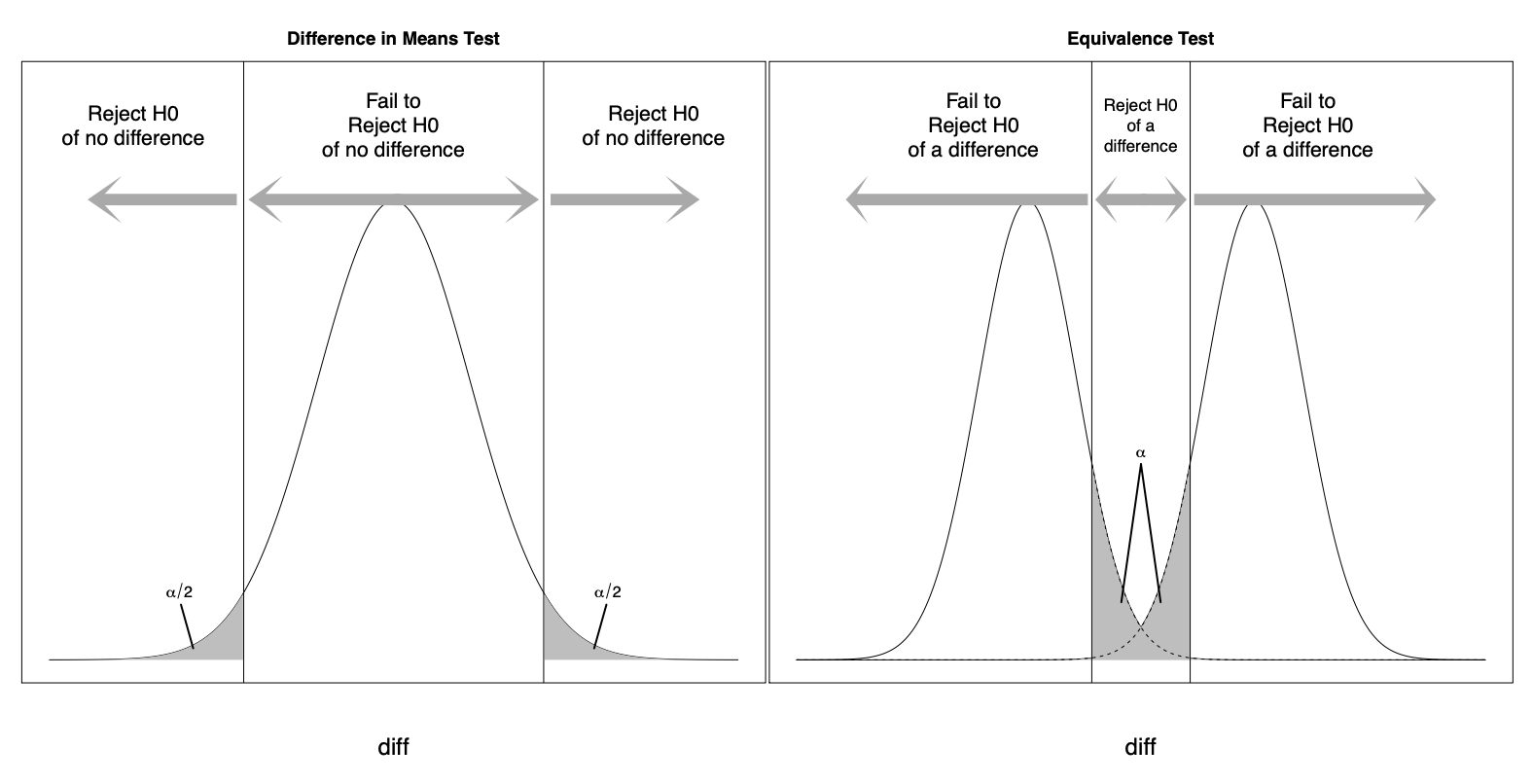
Figure A1: Figure 1 from [19] on the difference between the standard hypothesis testing and the equivalence testing.

Appendix G Simulation Study

We conduct a simulation study to compare the performance of the various DID estimators discussed in this paper. We demonstrate two key results. First, the double DID is unbiased under the extended parallel trends assumption or under the parallel trends-in-trends assumption. Second, the double DID has the smallest standard errors among unbiased DID estimators. In particular, standard errors of the double DID are smaller than those of the extended DID (i.e., the two-way fixed effects estimator) even under the extended parallel trends assumption.

We compare three DID estimators — the double DID, the extended DID, and the sequential DID — using two scenarios. In the first scenario, the extended parallel trends assumption (Assumption 2) holds where the difference between potential outcomes under control $\mathbb{E}[Y_{it}(0)\mid G_{i}=1]-\mathbb{E}[Y_{it}(0)\mid G_{i}=0]$ is constant over time. This corresponds to time-invariant unmeasured confounding, and we expect that all the DID estimators are unbiased in this scenario. The second scenario represents the parallel-trends-in-trends assumption (Assumption 3) where unmeasured confounding varies over time linearly. Here, we expect that the double DID and the sequential DID are unbiased, whereas the extended DID is biased.

For each of the two scenarios, we consider the balanced panel data with $n$ units and five-time periods where treatments are assigned at the last time period. We vary the number of units $(n)$ from $100$ to $1000$ and evaluate the quality of estimators by absolute bias and standard errors over 2000 Monte Carlo simulations. We describe the details of the simulation setup next.

G.1 Simulation Design

We consider the balanced panel data with $T=5$ ($t=\{0,1,2,3,4\}$) where the last period ($t=4$) is treated as the post-treatment period. We vary the number of units at each time period as $n\in\{100,250,500,1000\}$. Thus, the total number of observations are $nT\in\{500,1250,2500,5000\}$. We compare three estimators: the double DID, the extended DID, and the sequential DID.

Note that we consider four pre-treatment periods here, and thus the generalized double DID is not equal to the sequential DID even under the parallel trends-in-trends assumption because it combines two other moments and optimally weight them (see Appendix E.2). The equivalence between the sequential DID and the double DID holds only when there are two pre-treatment periods. We see below that the generalized double DID improves upon the sequential DID even under the parallel trends-in-trends assumption as they optimally weight observations from different time periods.

We study two scenarios: one under the extended parallel trends assumption (Assumption 2) and the other under the parallel-trends-in-trends assumption (Assumption 3). In the first scenario, the difference between potential outcomes under control $\mathbb{E}[Y_{it}(0)\mid G_{i}=1]-\mathbb{E}[Y_{it}(0)\mid G_{i}=0]$ is constant over time. In particular, we set

$$\mathbb{E}[Y_{it}(0)\mid G_{i}=g]=\alpha_{t}+0.05\times g$$ (A.6)

where $(\alpha_{0},\alpha_{1},\alpha_{2},\alpha_{3},\alpha_{4})=(1,2,3,4,5).$ In the second scenario, we allow for linear time-varying confounding. In particular, we set

$$\mathbb{E}[Y_{it}(0)\mid G_{i}=g]=\alpha_{t}+0.1\times g\times(t+1)$$ (A.7)

where $(\alpha_{0},\alpha_{1},\alpha_{2},\alpha_{3},\alpha_{4})=(1,2,3,4,5).$

Then, potential outcomes under control are drawn as follows. $Y_{it}(0)=\mathbb{E}[Y_{it}(0)\mid G_{i}]+\epsilon_{it}$ where $\epsilon_{it}$ follows the AR(1) process with autocorrelation parameter $\rho.$ That is,

$$\epsilon_{it} =\rho\epsilon_{i,t-1}+\xi_{it},$$

$$\epsilon_{i0} =\mathcal{N}(0,3/(1-\rho^{2})),$$

$$\xi_{it} =\mathcal{N}(0,3).$$

The causal effect is denoted by $\tau$ and thus, $Y_{it}(1)=\tau+Y_{it}(0)$ where we set $\tau=0.2.$ Finally, $Y_{it}=Y_{it}(0)$ for $t\leq 3$ (pre-treatment periods) and $Y_{it}=G_{i}Y_{it}(1)+(1-G_{i})Y_{it}(0)$ for $t=4$ (post-treatment period). The half of the samples are in the treatment group ($G_{i}=1$) and the other half is in the control group ($G_{i}=0$).

In Figure A2, we set the autocorrelation parameter $\rho=0.6$. This value is similar to the autocorrelation parameter used in famous simulation studies in [9] ($\rho=0.8$). We pick a smaller value to make our simulations harder as we see below. In Figure A3, we also provide additional results where we consider a full range of the autocorrelation parameters $\rho\in\{0,0.2,0.4,0.6,0.8\}$ (the same positive autocorrelation values considered in [9]). Both figures show the absolute bias and the standard errors which are defined as

$$\text{absolute bias}=\bigg{|}\frac{1}{M}\sum^{M}_{m=1}(\widehat{\tau}_{m}-\tau)\bigg{|}\quad\text{and}\quad\text{standard error}=\sqrt{\frac{1}{M}\sum^{M}_{m=1}(\widehat{\tau}_{m}-\tau)^{2}},$$

where $M$ is the total number of Monte Carlo iterations. Note that this standard error is a true standard error over the sampling distribution.

G.2 Results

Figure A2 shows the results when the autocorrelation parameter $\rho=0.6$. To begin with the absolute bias, visualized in the first row, all estimators have little bias under the extended parallel trends assumption (Scenario 1), as expected from theoretical results. In contrast, under the parallel-trends-in-trends assumption (Scenario 2), the extended DID (white circle with dotted line) is biased, while the double DID (black circle with solid line) and the sequential DID (white triangle with dotted line) are unbiased.

The second row represents the standard errors of each estimator. Under the extended parallel trends assumption (the first column), the double DID estimator has the smallest standard error, smaller than the extended DID estimator (i.e., the two-way fixed effects estimator). This efficiency gain comes from the fact that the double DID uses the GMM framework to optimally weight observations from different time periods, although the two-way fixed effects estimator uses equal weights to all pre-treatment periods.

Under the parallel trends-in-trends assumption (the second row; the second column), the double DID has almost the same standard error as the sequential DID. This shows that the double DID changes weights according to scenarios and solves a practical dilemma of the sequential DID — it is unbiased under the weaker assumption of the parallel trends-in-trends, but not efficient under the extended parallel trends.

Figure A2: Comparing DID estimators in terms of the absolute bias and the standard errors. The first row shows that the double DID estimator (black circle with solid line) is unbiased under both scenarios. The second row demonstrates that the double DID has the smallest standard errors among unbiased DID estimators.

In Figure A3, we provide additional results where we consider a full range of the autocorrelation parameters $\rho\in\{0,0.2,0.4,0.6,0.8\}$ (the same positive autocorrelation values considered in [9]). We find that when the autocorrelation of errors is small, standard errors of the double DID are smaller than those of the sequential DID even under the parallel trends-in-trends assumption.

Figure A3: Comparing DID estimators in terms of the absolute bias and the standard errors according to the autocorrelation of errors. Note: The first row shows that the double DID estimator (black circle with solid line) is unbiased under both scenarios. The second row demonstrates that the double DID has the smallest standard errors among unbiased DID estimators. Under the extended parallel trends assumption (the first column), the efficiency gain relative to the extended DID (i.e., two-way fixed effects estimator) is large when the autocorrelation parameter $\rho$ is large. Under the parallel trends-in-trends assumption (the second column), the efficiency gain relative to the sequential DID is large when $\rho$ is small.

The first row of Figure A3 shows that our results on the (absolute) bias do not change regardless of the autocorrelation of errors. In particular, the double DID is unbiased under the extended parallel trends assumption (the first column) or under the parallel trends-in-trends assumption (the second column). In terms of the standard errors (the second row), two results are important. First, under the extended parallel trends assumption (the first column), the standard errors of the double DID is the smallest for all the values of $\rho$ and the efficiency gain relative to the extended DID (i.e., two-way fixed effects estimator) is large when the there is high auto-correlations (i.e., $\rho$ is large). Second, under the parallel trends-in-trends assumption (the second column), the standard errors of the double DID is the smallest among unbiased DID estimators (the extended DID is biased). The efficiency gain relative to the sequential DID is large when $\rho$ is small.

Appendix H Empirical Application

H.1 Malesky, Nguyen, and Tran (2014): DID Design

In Section 3.4, we have focused on three outcomes to illustrate the advantage of the double DID estimator. Each outcome is defined as follows. “Education and Cultural Program” (binary): This variable takes one if there is a program that invests in culture and education in the commune. “Tap Water” (binary): What is the main source of drinking /cooking water for most people in this commune? “Agricultural Center” (binary): Is there any agriculture extension center in a given commune? Please see [30] for further details.

In this section, we provide results for all thirty outcomes analyzed in the original paper. To assess the underlying parallel trends assumptions, we combine visualization and formal tests, as recommended in the main text. The assessment suggests that we can make the extended parallel trends assumption for fifteen outcomes. Specifically, for those fifteen outcomes, p-values for the null of pre-treatment parallel trends are above 0.10 (i.e., fail to reject the null at the conventional level), and the 95% standardize equivalence confidence interval is contained in the interval $[-0.2,0.2]$. This means that the deviation from the parallel trends in the pre-treatment periods are less than 0.2 standard deviation of the control mean in 2006.

Figure A4 shows estimated treatment effects under the extended parallel trends assumption.

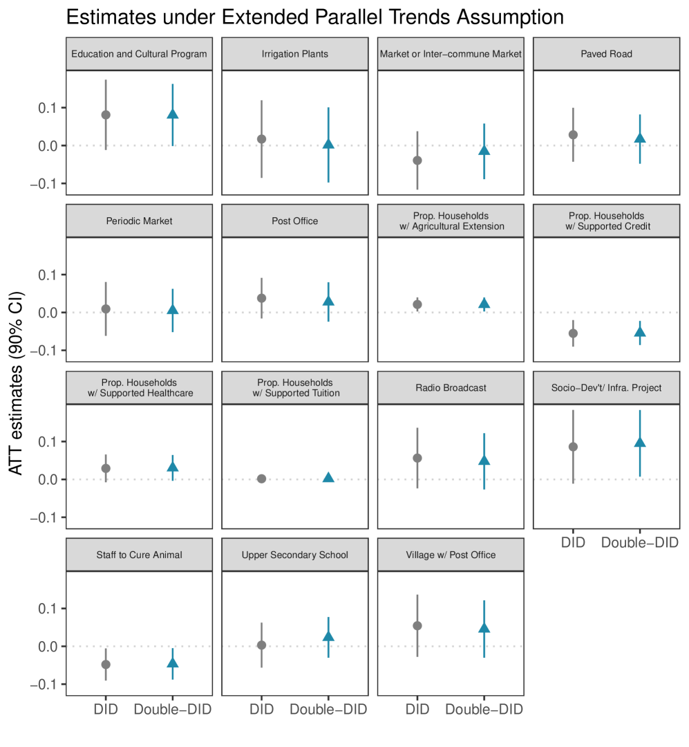
Figure A4: Comparing Standard DID and Double DID under Extended Parallel Trends Assumption. The double DID estimates are similar to those from the standard DID, and yet, standard errors are smaller because the double DID effectively uses pre-treatment periods within the GMM.

As in Section 3.4, the double DID estimates are similar to those from the standard DID, and yet, standard errors are smaller because the double DID effectively uses pre-treatment periods within the GMM. Here, we only have two pre-treatment periods, but when there are more pre-treatment periods, the efficiency gain of the double DID can be even larger.

We rely on the parallel trends-in-trends assumption for eight outcomes out of the fifteen remaining outcomes. These outcomes have the 95% standardized equivalence confidence interval wider than $[-0.20,0.20]$, but show that treatment and control groups’ pre-treatment trends have the same sign. The same sign of the pre-treatment trends suggests that parallel trends-in-trends assumption, which can account for the linear time-varying unmeasured confounder, can be plausible for these outcomes, even though the stronger parallel trends assumption is possibly violated.

Figure A5 shows results under the parallel trends-in-trends assumption. As in Section 3.4, the double DID estimates are often different from those of the standard DID because the extended parallel trends assumption is implausible for these outcomes. Importantly, standard errors of the double DID are often larger than the standard DID. This is because the double DID needs to adjust for biases in the standard DID by using pre-treatment trends.

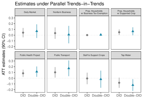
Figure A5: Comparing Standard DID and Double DID under Parallel Trends-in-Trends Assumption. The double DID estimates are often different from those of the standard DID because the extended parallel trends assumption is implausible for these outcomes.

For the remaining seven outcomes of which treatment and control groups’ pre-treatment trends have the opposite sign, it is difficult to justify either the extended parallel trends or parallel trends-in-trends assumption without additional information. Thus, there is no credible estimator for the ATT without making stronger assumptions. When there are more than two pre-treatment periods, researchers can apply the sequential DID estimator to pre-treatment periods in order to formally assess the extended parallel trends-in-trends assumption. We emphasize that, although we use the equivalence range of $[-0.20,0.20]$ as a cutoff for an illustration, it is recommended to base this decision on substantive domain knowledge whenever possible in practice.

H.2 Paglayan (2019): Staggered Adoption Design

In this section, we apply the proposed double DID estimator to revisit [34], which uses the staggered adoption (SA) design to study the effect of granting collective bargaining rights to teacher’s union on educational expenditures and teacher’s salary. [34] applies the standard two-way fixed effect models to estimate the effect of the introduction of the mandatory bargaining law in the US states on the two outcome. The original author exploits the variation induced by the different introduction timing of the law: A few states introduced the law as early as in the mid 1960’s, while some states, such as Arizona or Kentucky, never introduced the mandate. Among the states that granted the bargaining rights, the introduction timing varies from the mid 1960’s to the mid 1980’s (Nebraska was the last state that adopted the law).

H.2.1 Assessing Underlying Assumptions

We apply the proposed double DID for the SA design to the panel data consists of state-year observations. A state is treated at a particular year, if the state passes the law or has already passed the law of mandatory bargaining. Following the original study, we study two outcome: Per-pupil expenditure and annual teacher salary, both are on a log scale. There are 2,058 observations, containing 49 states (excluding Washington DC and Wisconsin, due to the short availability of the pre-treatment outcomes) and spanning from 1959 through 2000.

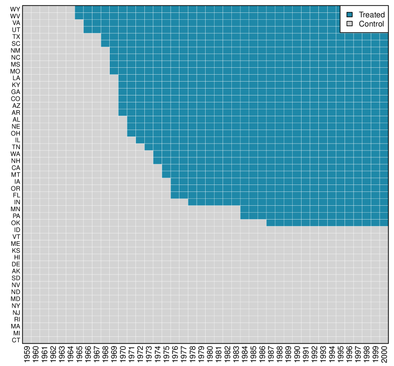
Figure A6: Treatment Variation Plot. Note: Cells in gray are state-year observations that are not treated (i.e., the mandatory bargaining law is not implemented), while cells in blue are observations that are under the treatment condition. Rows are sorted such that states that adopt the policy at earlier years are shown near the top, while states that never adopt the policy are shown near the bottom. The figure indicates that there are variations across states in adoption timings, and that some states never adopt the policy.

Figure A6 shows the variation of the treatment across states and over time. Cells in gray indicate state-year observations that are not treated and blue cells indicate the treated observations. We can observe that there are 14 unique treatment timings (the earliest is 1965 and the latest is 1987) where the number of states at each treatment timing varies from one to six (the average number of states at a treatment timing is 2.3). We can also see that there is no reversal of a treatment status in that once a state adopts the policy, the state has never abolished it during the sample period.

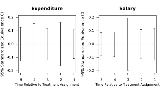
Figure A7: Assessing Underlying Assumptions Using the Pre-treatment Outcomes (Left: logged expenditure; Right: logged teacher salary). Note: We report the 95% standardized equivalence confidence intervals.

We assess the underlying parallel trends assumption for the SA design by utilizing the pre-treatment outcome. As in the pre-treatment-trends test in the basic DID design, we apply the standard DID estimator for the SA design to pre-treatment periods. For example, to test the pre-treatment trends from $t-1$ to $t$ for units who receive the treatment at time $t$, we estimate the SA-ATT using the outcome from $t-2$ and $t-1$ (See Section 4.2 for more details). To further facilitate interpretation, we standardize the outcome by the mean and standard deviation of the baseline control group, so that the effect can be interpreted relative to the control group.

Figure A7 shows 95% standardized equivalence confidence intervals for the two outcomes of interest (See Section 3.1 for details on the standardization procedure). It shows that for both outcomes, the equivalence confidence intervals are within 0.2 standard deviation from the means of the baseline control groups through $t-5$ to $t-1$. This suggests that the extended parallel trends assumption is plausible for both outcomes.

H.2.2 Estimating Causal Effects

We apply the double DID for the SA design as described in Section 4. The standard errors are computed by conducting the block bootstrap where the block is taken at the state level and we take 2000 bootstrap iterations. Analyses for the two outcomes are conducted separately. In addition to the proposed method, we apply two existing variants of synthetic control methods that can handle the staggered adoption design: the generalized synthetic control method, gsynth [40], and the augmented synthetic control method, augsynth [7]. While the proposed double DID is better suited for settings where there are a small to moderate number of pre-treatment periods, we evaluate, in the setting of long pre-treatment periods, whether it can achieve comparable performance to these variants of synthetic control methods that are primarily designed to deal with long pre-treatment periods (see more discussions in Section B.3).

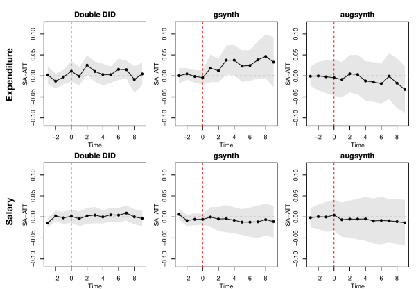
Figure A8: Plot of the Average Treatment Effect on the Treated on Two Outcomes. Note: We compare estimates from the double DID, the generalized synthetic control method, and the augmented synthetic control method. The causal estimates are similar across methods for both outcomes and treatment effects are not statistically significant at the conventional 5% level for most of the time periods.

Figure A8 shows the estimates of the treatment on the per-pupil expenditure (the first row) and the teacher’s salary (the second row), where both effects are on a log scale. We estimated the average treatment effect on the two outcomes $\ell$ periods after the treatment assignment where $\ell=\{0,1,\ldots,9\}.$ Note that $\ell=0$ corresponds to the contemporaneous effect. Each column corresponds to different estimators. The first column shows the proposed double DID estimator for the staggered adoption design, whereas the second (third) column shows estimates based on the generalized synthetic control method (the augmented synthetic control method). We can see that estimates are similar across methods for both outcomes and treatment effects are not statistically significant at the 5% level for most of the time periods. This result is consistent with the original finding of [34] that the granting collective bargaining rights did not increase the level of resources devoted to education.

As in this example, when there are a large number of pre-treatment periods, it is important to apply both synthetic control methods and the proposed double DID, and evaluate robustness across those approaches. This is critical because they rely on different identification assumptions. We found such robustness in this application, which provides us with additional credibility.

References

- [1] Alberto Abadie “Semiparametric Difference-in-Differences Estimators” In The Review of Economic Studies 72.1 Wiley-Blackwell, 2005, pp. 1–19
- [2] Alberto Abadie, Alexis Diamond and Jens Hainmueller “Synthetic Control Methods for Comparative Case Studies: Estimating the Effect of California’s Tobacco Control Program” In Journal of the American Statistical Association 105.490 Taylor & Francis, 2010, pp. 493–505
- [3] Joshua D Angrist and Jörn-Steffen Pischke “Mostly Harmless Econometrics: An Empiricist’s Companion” Princeton University Press, 2008
- [4] Susan Athey et al. “Matrix Completion Methods for Causal Panel Data Models” In Journal of the American Statistical Association Taylor & Francis, 2021
- [5] Susan Athey and Guido W Imbens “Design-based Analysis in Difference-in-Differences Settings with Staggered Adoption” In Journal of Econometrics Elsevier, 2021
- [6] Michael M Bechtel and Jens Hainmueller “How Lasting is Voter Gratitude? An Analysis of the Short-and Long-Term Electoral Returns to Beneficial Policy” In American Journal of Political Science 55.4 Wiley Online Library, 2011, pp. 852–868
- [7] Eli Ben-Michael, Avi Feller and Jesse Rothstein “Synthetic Controls and Weighted Event Studies with Staggered Adoption” In arXiv preprint arXiv:1912.03290, 2019
- [8] Eli Ben-Michael, Avi Feller and Jesse Rothstein “The Augmented Synthetic Control Method”, Available at https://arxiv.org/abs/1811.04170, 2018
- [9] Marianne Bertrand, Esther Duflo and Sendhil Mullainathan “How Much Should We Trust Differences-in-Differences Estimates?” In The Quarterly Journal of Economics 119.1 MIT Press, 2004, pp. 249–275
- [10] Will Bullock and Joshua D Clinton “More a Molehill Than a Mountain: The Effects of the Blanket Primary on Elected Officials’ Behavior from California” In The Journal of Politics 73.3 Cambridge University Press New York, USA, 2011, pp. 915–930
- [11] Brantly Callaway and Pedro H.C. Sant’Anna “Difference-in-Differences with Multiple Time Periods” In Journal of Econometrics Elsevier, 2020
- [12] Scott Cunningham “Causal Inference: The Mixtape” Yale University Press, 2021
- [13] Arindrajit Dube, Oeindrila Dube and Omar García-Ponce “Cross-Border Spillover: US Gun Laws and Violence in Mexico” In American Political Science Review 107.3 Cambridge University Press, 2013, pp. 397–417
- [14] John S Earle and Scott Gehlbach “The Productivity Consequences of Political Turnover: Firm-Level Evidence from Ukraine’s Orange Revolution” In American Journal of Political Science 59.3 Wiley Online Library, 2015, pp. 708–723
- [15] Francisco Garfias “Elite Competition and State Capacity Development: Theory and Evidence from Post-Revolutionary Mexico” In American Political Science Review 112.2 Cambridge University Press, 2018, pp. 339–357
- [16] Andrew Goodman-Bacon “Difference-in-Differences with Variation in Treatment Timing” In Journal of Econometrics Elsevier, 2021
- [17] Andrew B Hall “Systemic Effects of Campaign Spending: Evidence From Corporate Contribution Bans in US State Legislatures” In Political Science Research and Methods 4.2 Cambridge University Press, 2016, pp. 343–359
- [18] Lars Peter Hansen “Large Sample Properties of Generalized Method of Moments Estimators” In Econometrica 50.4 JSTOR, 1982, pp. 1029–1054
- [19] Erin Hartman and F Daniel Hidalgo “An Equivalence Approach to Balance and Placebo Tests” In American Journal of Political Science 62.4 Wiley Online Library, 2018, pp. 1000–1013
- [20] Chad Hazlett and Yiqing Xu “Trajectory Balancing: A General Reweighting Approach to Causal Inference with Time-Series Cross-Sectional Data”, Available at SSRN: https://ssrn.com/abstract=3214231, 2018
- [21] James Heckman, Hidehiko Ichimura, Jeffrey Smith and Petra Todd “Characterizing Selection Bias Using Experimental Data” In Econometrica 66.5 JSTOR, 1998, pp. 1017–1098
- [22] Kosuke Imai and In Song Kim “On the Use of Two-way Fixed Effects Regression Models for Causal Inference with Panel Data” In Political Analysis 29.3, 2021, pp. 405–415
- [23] Kosuke Imai and In Song Kim “When Should We Use Unit Fixed Effects Regression Models for Causal Inference with Longitudinal Data?” In American Journal of Political Science 63.2 Wiley Online Library, 2019, pp. 467–490
- [24] Guido W Imbens and Donald B Rubin “Causal Inference in Statistics, Social, and Biomedical Sciences” Cambridge University Press, 2015
- [25] Luke Keele and William Minozzi “How Much is Minnesota like Wisconsin? Assumptions and Counterfactuals in Causal Inference with Observational Data” In Political Analysis 21.2 Cambridge University Press, 2013, pp. 193–216
- [26] Jonathan McDonald Ladd and Gabriel S Lenz “Exploiting A Rare Communication Shift to Document the Persuasive Power of The News Media” In American Journal of Political Science 53.2 Wiley Online Library, 2009, pp. 394–410
- [27] Horacio Larreguy and John Marshall “The Effect of Education on Civic and Political Engagement in Nonconsolidated Democracies: Evidence from Nigeria” In Review of Economics and Statistics 99.3 MIT Press, 2017, pp. 387–401
- [28] Myoung-jae Lee “Generalized Difference in Differences With Panel Data and Least Squares Estimator” In Sociological Methods & Research 45.1 SAGE Publications Sage CA: Los Angeles, CA, 2016, pp. 134–157
- [29] Licheng Liu, Ye Wang and Yiqing Xu “A Practical Guide to Counterfactual Estimators for Causal Inference With Time-Series Cross-Sectional Data” In Available at SSRN 3555463, 2020
- [30] Edmund J Malesky, Cuong Viet Nguyen and Anh Tran “The Impact of Recentralization on Public Services: A Difference-in-Differences Analysis of the Abolition of Elected Councils in Vietnam” In American Political Science Review 108.1 Cambridge University Press, 2014, pp. 144–168
- [31] Michelle Marcus and Pedro H.C. Sant’Anna “The Role of Parallel Trends in Event Study Settings: An Application to Environmental Economics” In Journal of the Association of Environmental and Resource Economists 8.2 The University of Chicago Press Chicago, IL, 2021, pp. 235–275
- [32] Ricardo Mora and Iliana Reggio “Alternative Diff-in-Diffs Estimators with Several Pretreatment Periods” In Econometric Reviews 38.5 Taylor & Francis, 2019, pp. 465–486
- [33] Ricardo Mora and Iliana Reggio “Treatment Effect Identification Using Alternative Parallel Assumptions”, Working Paper 12-33 Economic Series (48), Universidad Carlos III. Available at https://e-archivo.uc3m.es/bitstream/handle/10016/16065/we1233.pdf?sequence=1, 2012
- [34] Agustina S Paglayan “Public-Sector Unions and the Size of Government” In American Journal of Political Science 63.1 Wiley Online Library, 2019, pp. 21–36
- [35] Xun Pang, Licheng Liu and Yiqing Xu “A Bayesian Alternative to Synthetic Control for Comparative Case Studies” In Political Analysis, 2021
- [36] Anton Strezhnev “Semiparametric Weighting Estimators for Multi-Period Difference-in-Differences Designs”, Presented at the 2018 American Political Science Association Meeting, 2018
- [37] Liyang Sun and Sarah Abraham “Estimating Dynamic Treatment Effects in Event Studies with Heterogeneous Treatment Effects” In Journal of Econometrics Elsevier, 2020
- [38] Rory Truex “The Returns to Office in a “Rubber Stamp” Parliament” In American Political Science Review 108.2 Cambridge University Press, 2014, pp. 235–251
- [39] Stefan Wellek “Testing Statistical Hypotheses of Equivalence and Noninferiority” ChapmanHall/CRC, 2010
- [40] Yiqing Xu “Generalized Synthetic Control Method: Causal Inference with Interactive Fixed Effects Models” In Political Analysis 25.1 Cambridge University Press, 2017, pp. 57–76