Instrumental Variable Value Iteration for Causal Offline Reinforcement Learning

Abstract

In offline reinforcement learning (RL) an optimal policy is learned solely from a priori collected observational data. However, in observational data, actions are often confounded by unobserved variables. Instrumental variables (IVs), in the context of RL, are the variables whose influence on the state variables are all mediated through the action. When a valid instrument is present, we can recover the confounded transition dynamics through observational data. We study a confounded Markov decision process where the transition dynamics admit an additive nonlinear functional form. Using IVs, we derive a conditional moment restriction (CMR) through which we can identify transition dynamics based on observational data. We propose a provably efficient IV-aided Value Iteration (IVVI) algorithm based on a primal-dual reformulation of CMR. To the best of our knowledge, this is the first provably efficient algorithm for instrument-aided offline RL.

1 Introduction

In reinforcement learning (RL) [64], an agent maximizes its expected total reward by sequentially interacting with the environment. RL algorithms have been applied in the healthcare domain to dynamically suggest optimal treatments for patients with certain diseases [60, 37, 27, 50, 28, 55, 58].

One of the major concerns of working with observational data, especially for RL applications in healthcare, is confounding caused by unobserved variables. Because the available data may not contain measurements of important prognostic variables that guide treatment decisions, or heuristic information such as visual inspection of or discussions with patients during each treatment period, variables that affect both the treatment decisions and the next-stage health status of patients are present. See [11] for a detailed discussion of sources of confounding in healthcare datasets.

Instrumental variables (IVs) are a very well-known tool in econometrics and causal inference to identify causal effects in the presence of unobserved confounders (UCs). Informally, a variable $Z$ is an IV for the causal effect of the treatment variable $X$ on the outcome variable $Y$, if (i) it is correlated with $X$, and (ii) $Z$ only affects $Y$ through $X$. IVs are commonly used in healthcare studies to identify the effects of a treatment or intervention on health outcomes. There are some common sources of IVs in the medical literature, such as the preference-based IVs (see Example A.1), distance to a specialty care provider, and genetic variants [3]. We introduce one example below.

Example 1.1 (Differential travel time as IV, NICU application).

[41, 46, 18] study the effect on neonatal mortality of delivery at high-level neonatal intensive care units (NICU), using the same differential travel time as IV. The goal is to design a neonatal regionalization system that designates hospitals according to the level of care infants need. The available dataset has $\sim$180,000 records of mothers who delivered exactly two births during 1995 and 2009 in Pennsylvania and relocated at the second delivery. In Figure 1 we present a possible causal DAG for the NICU application. UCs are present due to mothers’ self-selection effects or unrecorded side information on which the physicians base the NICU suggestion. The differential travel time to the closest high-level NICU versus low-level NICU serves as a valid IV since it affects mothers’ choice of NICU and does not impact clinical outcomes through other means. A neonatal regionalization system (Figure 1, right panel) designates NICU solely based on the clinical outcome at the previous stage (since differential travel time does not affect clinical outcome anymore once we actually assign NICU, and confounders remain unobserved), removing arrows pointing into NICU decision in the DAG presented in the upper panel.

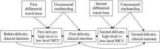
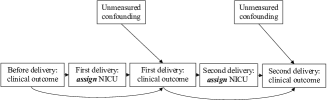
Figure 1: The NICU application, adapted from [18, Figure 1]. Left panel: DAG representing data generation process where UCs are present. Right panel: DAG representing a prenatal regionalization system in action.

We summarize three aspects of offline medical datasets often encountered by RL practitioners: (i) there is a large amount of logged data where the actual effects of medical treatment on patient’s health are confounded, (ii) the potential presence of a valid IV has been argued for in the biostatistics and epidemiology literature, and (iii) it is expensive or unethical to do experimentation and then inspect the actual performance of a target treatment policy. We ask

When a valid IV is present, can we design a provably efficient offline RL
algorithm using only confounded observational data?

We answer this question affirmatively. We formulate the sequential decision-making process in the presence of both IVs and UCs through a model we termed Confounded Markov Decision Process with Instrumental Variables (CMDP-IV). We then propose an IV-aided Value Iteration (IVVI) algorithm to recover the optimal policy through a model-based approach. Our contribution is threefold. First, under the additive UC assumption, we derive a conditional moment restriction through which we point identify transition dynamics. Second, we reformulate the conditional moment restriction as a primal-dual optimization problem, and propose an estimation procedure that enjoys computational and statistical efficiency jointly. Finally, we show that the sample complexity of recovering an $\epsilon$-optimal policy using observational data with IVs is $O(\mu_{\operatorname*{IV}}^{-4}\mu_{B}^{-2.5}H^{4}d_{x}\epsilon^{-2})$, where $0<\mu_{\operatorname*{IV}}<1$ quantifies the strength of the IV, $\mu_{B}$ is the minimum eigenvalue of the dual feature covariance matrix, quantifying the compatibility of the dual linear function space and the IV, $H$ is the horizon of the MDP, and $d_{x}$ is the dimension of states. To the best of our knowledge, this is the first sample complexity result for an IV-aided offline RL.

1.1 Related Work

RL in the presence of UCs has attracted increasing attention; see §A for a detailed overview of related work. One major difficulty of working with unobserved confounders is the issue of identification. When unobserved confounders are present, causal effects of actions are not identifiable from data without further assumptions. In these settings, several approaches are available. The first one is the sensitivity-analysis based approach [62], where we posit additional sensitivity assumptions on how strong the unobserved confounding can possibly be. These sensitivity assumptions enable partial identification of the causal quantity. This approach is employed by a sequence of work in [36, 34, 35, 50]. The second approach is to assume access to other auxiliary variables that can enable point or partial identification. We adopt the second approach in this work, by assuming the access to instrumental variables. Under an additive UC assumption (see (2.6)), instrumental variables can enable point identification of the structural quantity through conditional moment restriction (along with certain completeness assumptions; see Remark C.1), allowing us to work with continuous actions and continuous IVs. For example, in the NICU application, differential travel time (the IV) is a continuous quantity. Note that several other related works also study the use of instrumental variables [59, 18]. These works, and in particular [18], rely on partial identification bounds in the fully nonparametric IV setting [44, 4]. These bounds are only available for binary IVs or binary treatments, restricting the use of their algorithms in many real-world scenarios where the IV is continuous. A continuous IV like the differential travel time must be dichotomized if one were to apply these algorithms.

1.2 Notation

We use $\|\cdot\|_{2}$ to denote the $\ell_{2}$-norm of a vector or the spectral norm of a matrix, and use $\|\cdot\|_{F}$ to denote the Frobenius norm of a matrix. For vectors $a,b$ of the same length, let $a\cdot b$ denote the inner product. We denote by $\Delta(\mathcal{M};{\mathcal{N}})$ the set of distributions on $\mathcal{M}$ indexed by elements in ${\mathcal{N}}$. For a real symmetric matrix $A$, let $\sigma_{\text{max}}(A)$ and $\sigma_{\text{min}}(A)$ be its largest and smallest eigenvalues, respectively. For any positive integer $n$, we define $[n]=\{1,\dots,n\}$. For any bounded function $\varphi\colon{\mathcal{X}}\to\mathbb{R}^{d_{\varphi}}$, we define the linear function space spanned by $\varphi$ as $\mathcal{H}_{\varphi}=\{\theta\cdot\varphi\colon\theta\in{{\mathbb{R}}}^{d_{\varphi}}\}$. For any function $f=\theta\cdot\varphi\in\mathcal{H}_{\varphi}$, we denote by $\|f\|_{\varphi}=\|\theta\|_{2}$ its norm.

2 Problem Setup

We formulate the problem in this section. We first define instrumental variables (IVs) in §2.1 as a preliminary. In §2.2.1, we describe the evaluation setting, where we test the performance of our learned policy. In §2.2.2, we describe the offline setting in which we collect the observational data to learn a policy. Our goal is then to recover the optimal policy for the evaluation setting, using only data collected in the offline setting.

2.1 Preliminaries: Instrumental Variables

We define confounders and IVs as follows.

Definition 2.1 (Confounders and Instrumental Variables, [56]).

A variable $\varepsilon$ is a confounder relative to the pair $(X,Y)$ if $(X,Y)$ are both caused by $\varepsilon$. A variable $Z$ is an IV relative to the pair $(X,Y)$, if it satisfies the following two conditions: (i) $Z$ is independent of all variables that have influence on $Y$ and are not mediated by $X$; (ii) $Z$ is not independent of $X$.

Figure 2 (left panel) illustrates a typical causal directed acyclic graph (DAG) for an IV, where $Z$ is the IV relative to the pair $(X,Y)$, and $\varepsilon$ is the UC relative to the pair $(X,Y)$. The the DAG in Figure 2 (left) can also be characterized by $X=g(Z,\varepsilon)$ and $Y=f(X,\varepsilon)$ given independent $Z$ and $\varepsilon$, where $f$ and $g$ are two deterministic functions.

2.2 CMDP-IV

We first introduce a type of finite-horizon Markov Decision Process (MDP) in the offline setting with UCs and IVs, which we term Confounded Markov Decision Process with Instrumental Variables (CMDP-IV). CMDP-IV is a natural extension of the IV model introduced in §2.1 to the multi-stage decision making process. In §B we discuss possible extension of this model.

A CMDP-IV is defined as a tuple $M=({\mathcal{S}},\mathcal{A},\mathcal{Z},\mathcal{U},H,r;\xi_{0},{\mathcal{P}}_{e},{\mathcal{P}}_{z},F^{*},\pi_{b})$, where the sets ${\mathcal{S}}\subseteq{{\mathbb{R}}}^{d_{x}}$ and $\mathcal{A}$ are state and action spaces; the set $\mathcal{Z}\subseteq\mathbb{R}^{d_{z}}$ is the space of IVs; the set $\mathcal{U}\subseteq{{\mathbb{R}}}^{d_{x}}$ is the space of UCs; the integer $H$ is the length of each episode; and $r=\{r_{h}:{\mathcal{S}}\times\mathcal{A}\to[0,1]\}_{h=1}^{H}$ is the set of deterministic reward functions, where $r_{h}$ is the reward function at the $h$-th step. For simplicity of presentation, we assume that the reward function $r_{h}$ is known for any $h\in[H]$. Furthermore, $\xi_{0}\in\Delta({\mathcal{S}})$ is the initial state distribution, ${\mathcal{P}}_{e}=\mathcal{N}(0,\sigma^{2}I_{d_{x}})$ is the distribution of UCs, and ${\mathcal{P}}_{z}$ is the distribution of IVs. The function $F^{*}:{\mathcal{S}}\times\mathcal{A}\to{\mathcal{S}}$ is a deterministic transition function and $\pi_{b}=\{\pi_{b,h}\in\Delta(\mathcal{A};{\mathcal{S}},\mathcal{Z},\mathcal{U})\}_{h=1}^{H}$ is the behavior policy, where $\pi_{b,h}$ is the behavior policy at the $h$-th step.

2.2.1 Evaluation setting: Bellman Equations and Performance Metric

We now introduce the evaluation setting of CMDP-IV. The evaluation setting is the same as the usual RL setup [64]: we want to find an optimal policy in the MDP.

For a policy $\pi=\{\pi_{h}\in\Delta(\mathcal{A};{\mathcal{S}})\}_{h=1}^{H}$, given an initial state $x_{1}\sim\xi_{0}$, for any $h\in[H]$, the dynamics in an evaluation setting at the $h$-th step is

$$a_{h}\sim\pi_{h}(\cdot{\,|\,}x_{h}),\quad x_{h+1}=F^{*}(x_{h},a_{h})+e_{h},$$ (2.1)

where $\{e_{h}\}_{h=1}^{H}\stackrel{{\scriptstyle{\scriptscriptstyle\operatorname*{iid}}}}{{\sim}}{\mathcal{P}}_{e}$ is the sequence of Gaussian innovations. The episode terminates if we reach the state $x_{H+1}$. For simplicity, for any $F:{\mathcal{S}}\times\mathcal{A}\to{{\mathbb{R}}}^{d_{x}}$ we define the following transition kernel

$${\mathcal{P}}_{F}(\cdot{\,|\,}x_{h},a_{h})=\mathcal{N}(F(x_{h},a_{h}),\sigma^{2}I_{d_{x}}).$$ (2.2)

We define the value function and the Q-function of a policy under the evaluation setting (2.1). For any $h\in[H]$, given any policy $\pi_{h}$ at the $h$-th step, we define its value function $V^{\pi}_{h}:{\mathcal{S}}\rightarrow\mathbb{R}$ and its Q-function $Q^{\pi}_{h}:{\mathcal{S}}\times\mathcal{A}\rightarrow{{\mathbb{R}}}$ as follows,

$$V^{\pi}_{h}(x)\vcentcolon=\mathbb{E}_{\pi}\Bigl{[}\sum_{i=h}^{H}r_{i}(x_{i},a_{i})\,\Big{|}\,x_{h}=x\Bigr{]},\,\,\,Q_{h}^{\pi}(x,a)\vcentcolon=\mathbb{E}_{\pi}\Bigl{[}\sum_{i=h}^{H}r_{i}\left(x_{i},a_{i}\right)\Big{|}x_{h}=x,a_{h}=a\Bigr{]}.$$ (2.3)

Here, the expectation $\mathbb{E}_{\pi}$ is taken with respect to the randomness of the state-action sequence $\{(x_{i},a_{i})\}_{i=h}^{H}$, where the action $a_{i}$ follows the policy $\pi_{i}(\cdot\,|\,x_{i})$ and the next state $x_{i+1}$ follows the transition kernel ${\mathcal{P}}_{F^{*}}(\cdot\,|\,x_{i},a_{i})$ defined in (2.2) for any $i\in\{h,h+1,\ldots,H\}$.

An optimal policy $\pi^{*}$ gives the optimal value $V_{h}^{*}(x)=\sup_{\pi}V_{h}^{\pi}(x)$ for any $(x,h)\in{\mathcal{S}}\times[H]$. We assume that such an optimal policy $\pi^{*}$ exists. For a given policy $\pi=\{\pi_{h}\in\Delta(\mathcal{A};{\mathcal{S}})\}_{h=1}^{H}$, its suboptimality compared to the optimal policy $\pi^{*}=\{\pi_{h}^{*}\}_{h=1}^{H}$ is defined as

$$\|V^{*}_{1}-V^{\pi}_{1}\|_{\infty}\coloneqq\sup_{x\in{\mathcal{S}}}V^{*}_{1}(x)-V^{\pi}_{1}(x).$$ (2.4)

We describe the Bellman equation and the Bellman optimality equation for the evaluation setting. For any $(x,a,h)\in\mathcal{S}\times\mathcal{A}\times[H]$, the Bellman equation of the policy $\pi$ takes the following form,

$$Q^{\pi}_{h}(x,a)=(r_{h}+\mathbb{P}V^{\pi}_{h+1})(x,a),\quad V^{\pi}_{h}(x)=\langle Q^{\pi}_{h}(x,\cdot),\pi_{h}(\cdot\,|\,x)\rangle_{\mathcal{A}},\quad V^{\pi}_{H+1}(x)=0,$$

where $\langle Q^{\pi}_{h}(x,\cdot),\pi_{h}(\cdot\,|\,x)\rangle_{\mathcal{A}}=\int_{\mathcal{A}}Q_{h}^{\pi}(x,a)\pi_{h}({\mathrm{d}}a\,|\,x)$ and $\mathbb{P}$ is the operator form of the transition kernel ${\mathcal{P}}_{F^{*}}$, i.e., defined as $({\mathbb{P}}f)(x,a)=\mathbb{E}_{x^{\prime}\sim{\mathcal{P}}_{F^{*}}(\cdot\,|\,x,a)}[f(x^{\prime})]$ for any function $f:{\mathcal{S}}\rightarrow{{\mathbb{R}}}$. The subscript $\mathcal{A}$ is omitted subsequently if it is clear from the context. Similarly, the Bellman optimality equation takes the following form,

$$Q_{h}^{*}(x,a)=(r_{h}+\mathbb{P}V_{h+1}^{*})(x,a),\quad V_{h}^{*}(x)=\max_{a\in\mathcal{A}}Q_{h}^{*}(x,a),\quad V_{H+1}^{*}(x)=0,$$ (2.5)

which implies that to find an optimal policy $\pi^{*}$, it suffices to estimate the optimal Q-function and then construct the greedy policy with respect to the optimal Q-function.

2.2.2 Offline Setting: Data Collection Process

We describe the offline setting of CMDP-IV, in which we collect the data by executing the behavior policy $\pi_{b}\in\Delta(\mathcal{A};{\mathcal{S}},\mathcal{Z},\mathcal{U})^{H}$. This distinguishes our work from most works in offline RL since we need to handle the issue of unobserved confounders, which makes the already difficult offline RL problem even more challenging.

At the beginning of each episode, the environment generates an initial state $x_{1}\sim\xi_{0}$, a sequence of UCs $\{e_{h}\}_{h}\stackrel{{\scriptstyle{\scriptscriptstyle\operatorname*{iid}}}}{{\sim}}{\mathcal{P}}_{e}$, and a sequence of observable IVs $\{z_{h}\}_{h}\stackrel{{\scriptstyle{\scriptscriptstyle\operatorname*{iid}}}}{{\sim}}{\mathcal{P}}_{z}$. At the $h$-th step, given the current state $x_{h}$, the action $a_{h}$ and the next state $x_{h+1}$ are generated according to the following dynamics,

$$a_{h}\sim\pi_{b,h}(\cdot{\,|\,}x_{h},z_{h},e_{h}),\quad x_{h+1}=F^{*}(x_{h},a_{h})+e_{h}.$$ (2.6)

The episode terminates if we reach the state $x_{H+1}$ and we collect all observable variables, i.e., $\{(x_{h},a_{h},z_{h},x_{h}^{\prime})\}_{h\in[H]}$, where $x_{h}^{\prime}=x_{h+1}$ for any $h\in[H]$.

A causal DAG is given in Figure 2 (left) to graphically illustrate such dynamics. At any stage $h$, the variable $z_{h}$ is an IV relative to the pair $(a_{h},x_{h+1})$. Indeed, $z_{h}$ affects the action $a_{h}$ only through (2.6), and its effect on $x_{h+1}$ must be channelled through $a_{h}$ because it does not appear in the second equation in (2.6).

The main difference between the evaluation setting (2.1) and the offline setting (2.6) is whether the UC $e_{h}$ has an effect on the action $a_{h}$. In the language of causal inference [56], a policy $\pi=\{\pi_{h}\in\Delta(\mathcal{A};{\mathcal{S}})\}_{h=1}^{H}$ induces the stochastic intervention $\operatorname{do}(a_{1}\sim\pi_{1}(\cdot{\,|\,}x_{1}),\dots,a_{H}\sim\pi_{H}(\cdot{\,|\,}x_{H}))$ on the DAG in Figure 2 (left part of the right panel), and the resulting DAG is obtained by removing all arrows pointing into the action $a_{h}$; see Figure 2 (right part of the right panel). §E includes more details on the do-operation.

Under the offline and the evaluation settings described in Sections 2.2.2 and 2.2.1, respectively, we aim to answer the following question:

Given data collected from the confounded dynamics (2.6) in the offline setting, can we find a policy that minimizes the suboptimality defined in (2.4) in the evaluation setting?

The challenge of the problem stems from the fact that the UC $e_{h}$ enters both of the equations (2.6). In general we do not have ${\mathbb{E}}[x_{h+1}\,|\,x_{h},a_{h}]=F^{*}(x_{h},a_{h})$ in the offline dynamics; see Remark B.3.

     

Figure 2: Left panel: An illustration of Definition 2.1 with one UC $\varepsilon$ and three observable variables $X$, $Y$, and $Z$. Right panel: Offline setting of CMDP-IV with a behavior policy $\pi_{b}$ (left). Evaluation setting of CMDP-IV with intervention induced by $\pi$ (right).

3 IV-Aided Value Iteration

How can an IV help us design an offline RL algorithm? To answer this question, we proceed by a model-based approach. We estimate the transition function $F^{*}$ first. And then any planning algorithm (value iteration in our case) can be used to recover the optimal policy under the evaluation setting.

3.1 A Primal-Dual Estimand

We observe that, thanks to the presence of IVs, the transition function $F^{*}$ is the solution of a conditional moment restriction (CMR). To estimate the transition function $F^{*}$ based on the CMR, we derive a primal-dual formulation of the CMR in §3.1.2.

3.1.1 Conditional Moment Restriction

Following the confounded dynamics (2.6), the behavior policy $\pi_{b}$ induces the distribution of the observable trajectories $\{x_{h},a_{h},z_{h},x^{\prime}_{h}=x_{h+1}\}_{h=1}^{H}$. We denote by $d_{h,\pi_{b}}$ the distribution of the tuple $(x_{h},a_{h},z_{h},x^{\prime}_{h})\in{\mathcal{S}}\times\mathcal{A}\times\mathcal{Z}\times{\mathcal{S}}$ at the $h$-th step for any $h\in[H]$, i.e., $d_{h,\pi_{b}}(x,a,z,x^{\prime})$. We further define the average visitation distribution as follows,

$$\bar{d}_{\pi_{b}}(x,a,z,x^{\prime})=\frac{1}{H}\cdot\sum_{h=1}^{H}d_{h,\pi_{b}}(x,a,z,x^{\prime})$$ (3.1)

for any $(x,a,z,x^{\prime})\in{\mathcal{S}}\times\mathcal{A}\times\mathcal{Z}\times{\mathcal{S}}$. We denote by ${L^{2}({\mathcal{S}},\mathcal{A})}=\{f\colon{\mathcal{S}}\times\mathcal{A}\to{{\mathbb{R}}},\leavevmode\nobreak\ {\mathbb{E}}[f(x,a)^{2}]<\infty\}$ the space of square integrable functions equipped with the norm $\|f\|^{2}_{{L^{2}({\mathcal{S}},\mathcal{A})}}={\mathbb{E}}[f(x,a)^{2}]$. Similarly, we define ${L^{2}(\mathcal{Z})}$ and the norm $\|g\|^{2}_{{L^{2}(\mathcal{Z})}}={\mathbb{E}}[g(z)^{2}]$. The operator ${\mathcal{T}}\colon{L^{2}({\mathcal{S}},\mathcal{A})}\to{L^{2}(\mathcal{Z})}$ is defined as

$$({\mathcal{T}}f)(\cdot)={\mathbb{E}}[f(x,a){\,|\,}z=\cdot\,].$$ (3.2)

The following proposition states the conditional moment restriction (CMR) implied by the IVs in the offline confounder dynamics (2.6). See §F.1 for the proof.

Proposition 3.1 (CMR).

If $(x,a,z,x^{\prime})$ is distributed according to the law $\bar{d}_{\pi_{b}}$, then for any $z\in\mathcal{Z}$,

$${\mathbb{E}}[F^{*}(x,a){\,|\,}z]={\mathbb{E}}[x^{\prime}{\,|\,}z]\,.$$ (3.3)

Proposition 3.1 implies that the transition function $F^{*}$ satisfies the equation ${\mathcal{T}}F^{*}={\mathbb{E}}[x^{\prime}{\,|\,}z]$, where the operator ${\mathcal{T}}$ is defined in (3.2). Such an equation is a Fredholm integral equation of the first kind [38]. Given data collected from $\bar{d}_{\pi_{b}}$, we aim to estimate $F^{*}$ based on the CMR.

Remark 3.2 (Global IVs and global UCs).

Our method directly extends to cases where, instead of a time-varying IV, we only have access to a global IV that affects all the actions taken on a trajectory simultaneously, e.g. a doctor’s preference to certain treatments. The reason is that the global IV, conditional on the past history, is also a valid IV for each time step, mimicking the structure of the time-varying IV. Specifically, having a global IV is equivalent to having $z_{h}=z$ for all $h$, i.e. all local IVs take the same value. Then, by the full independence between $\{e_{h}\}_{h}$ and $z$, the core requirement of the time-varying IV ${\mathbb{E}}[e_{h}\,|\,z]=0$ still holds, and thus our result applies.

Our model can also be extended to the case of global UCs, assuming that the global UCs have the same effect on the states $x_{h}$ in both offline and evaluation settings. Only their effects on the actions $a_{h}$ can differ; the global UCs affect the actions offline but not in evaluation setting. In more detail, the global UCs affect all stages of decision making, and thus affect all states $x_{h}$ and actions $a_{h}$. While IV can deconfound the effects of global UCs on the actions $a_{h}$, it cannot deconfound their effects on the states $x_{h},x_{h+1}$. The transition dynamics from $x_{h}$ to $x_{h+1}$ would depend on the global UCs. This dependence would limit the performance of the learned policy in evaluation settings if the evaluation transition dynamics from $x_{h}$ to $x_{h+1}$ does not depend on the global UCs in the same way. Yet, assuming that the effect of global UCs on the states are persistent in both evaluation and offline settings, our results would extend to global UCs. Moreover, with additional assumptions on the transition dynamics, some settings of global UCs can be reduced to our setting. For example, suppose the dynamics for stage $h$ write

$$a_{h}\sim\pi_{b}(\cdot\,|\,x_{h},z_{h},e),\quad x_{h+1}=F^{*}(x_{h},a_{h})+e,$$

where the UC at each stage is identical and is denoted $e$. One can difference the sequence $\{x_{h}\}_{h}$, and obtain $x_{h+1}-x_{h}=F^{*}(x_{h},a_{h})-F^{*}(x_{h-1},a_{h-1})$, where the global UC is cancelled. Due to these considerations, we focus on the CMDP-IV setting in this work, which itself is a natural extension of the IV model introduced in §2.1 to the multi-stage decision making process.

3.1.2 A Primal-Dual Estimand

We derive a primal-dual estimand for $F^{*}=[f_{1}^{*},\dots,f_{d_{x}}^{*}]^{\top}$. For any $i\in[d_{x}]$, by Proposition 3.1, ${\mathbb{E}}[f^{*}_{i}(x,a){\,|\,}z]={\mathbb{E}}[x^{\prime}_{i}{\,|\,}z],$ where $x^{\prime}_{i}$ is the $i$-th element of the next state $x^{\prime}$. We find $f^{*}_{i}$ by solving the least-square problem $\min_{f_{i}\in{L^{2}({\mathcal{S}},\mathcal{A})}}\tfrac{1}{2}{\mathbb{E}}[({\mathbb{E}}[f_{i}(x,a){\,|\,}z]-{\mathbb{E}}[x^{\prime}_{i}{\,|\,}z])^{2}].$ By Fenchel duality, the least-square problem admits a primal-dual formulation

$$\min_{f_{i}\in{L^{2}({\mathcal{S}},\mathcal{A})}}\max_{u_{i}\in{L^{2}(\mathcal{Z})}}{\mathbb{E}}[(f_{i}(x,a)-x^{\prime}_{i})u_{i}(z)]-\tfrac{1}{2}{\mathbb{E}}[u_{i}(z)^{2}]\,,$$ (3.4)

where $u_{i}$ is the dual variable. To approximate the $L^{2}$ spaces, we introduce two known feature maps

$$\phi\colon{\mathcal{S}}\times\mathcal{A}\to{{\mathbb{R}}}^{d_{\phi}},\quad\psi\colon\mathcal{Z}\to{{\mathbb{R}}}^{d_{\psi}},$$

and let $\mathcal{H}_{\phi}$ and $\mathcal{H}_{\psi}$ denote the spaces spanned by $\phi$ and $\psi$, respectively. For simplicity, we define the following uncentered covariance matrices

$$A={\mathbb{E}}[\psi(z)\phi(x,a)^{\top}],\,\,B={\mathbb{E}}[\psi(z)\psi(z)^{\top}],\,\,C={\mathbb{E}}[x^{\prime}\psi(z)^{\top}],\,\,D={\mathbb{E}}[\phi(x,a)\phi(x,a)^{\top}].$$ (3.5)

where the expectations are taken following $\bar{d}_{\pi_{b}}$. We replace the $L^{2}$ spaces in (3.4) by their finite-dimensional subspaces, $\min_{f_{i}\in\mathcal{H}_{\phi}}\max_{u_{i}\in\mathcal{H}_{\psi}}{\mathbb{E}}[(f_{i}(x,a)-x^{\prime}_{i})u_{i}(z)]-\tfrac{1}{2}{\mathbb{E}}[u_{i}(z)^{2}]\,,$ which, in matrix form, writes

$$\min_{\theta_{i}\in{{\mathbb{R}}}^{d_{\phi}}}\max_{\omega_{i}\in{{\mathbb{R}}}^{d_{\psi}}}\,\omega_{i}^{\top}A\theta_{i}-b_{i}\omega_{i}-\tfrac{1}{2}\omega_{i}^{\top}B\omega_{i}\,,$$ (3.6)

where $b_{i}\vcentcolon={\mathbb{E}}[x_{i}^{\prime}\psi(z)^{\top}]$ and $A$ and $B$ are defined in (3.5). We address the approximation error incurred by such finite-dimensional approximation in §4.2. Now we collect (3.6) for all coordinates $i\in[d_{x}]$, giving the key primal-dual estimand ${W^{\operatorname*{sad}}}$

$${W^{\operatorname*{sad}}}\vcentcolon=\mathop{\mathrm{argmin}}_{W}\max_{K}\,L(W,K),$$ (3.7)

where $L(W,K)\vcentcolon={\text{Tr}}(KAW^{\top})-{\text{Tr}}(CK^{\top})-\tfrac{1}{2}{\text{Tr}}(KBK^{\top})$ with $W=[\theta_{1},\dots,\theta_{d_{x}}]^{\top}\in\mathbb{R}^{d_{x}\times d_{\phi}}$ and $K=[\omega_{1},\dots,\omega_{d_{x}}]^{\top}\in\mathbb{R}^{d_{x}\times d_{\psi}}$. For carefully chosen feature maps we expect ${W^{\operatorname*{sad}}}\phi\approx F^{*}$.

3.2 Algorithm

We first introduce the following data sampling assumption for the algorithm.

Assumption A.1 (Offline data).

We have access to i.i.d. data from the average visitation distribution defined in (3.1). That is, $\{(x_{t},a_{t},z_{t},x^{\prime}_{t})\}_{t=0}^{T-1}\stackrel{{\scriptstyle{\scriptscriptstyle\operatorname*{iid}}}}{{\sim}}\bar{d}_{\pi_{b}}$.

Assumption A.1 is only used to simplify the presentation of our results, by ignoring the temporal dependence in the data.

Algorithm 1 introduces the backbone of the paper, IV-aided Value Iteration (IVVI), which recovers the optimal policy under the evaluation setting given data collected from the confounded dynamics under the offline setting. Algorithm 1 consists of the following two phases.

Algorithm 1 IV-aided Value Iteration (IVVI)

1:  Input: Reward functions $\{r_{h}\}_{h=1}^{H}$, feature maps $\phi$ and $\psi$, iterations $T$, stepsizes $\{\eta_{t}^{\theta},\eta_{t}^{\omega}\}_{t=1}^{T}$, initial estimates $K_{0}$ and $W_{0}$, variance $\sigma^{2}$, samples $\{(x_{t},a_{t},z_{t},x^{\prime}_{t})\}_{t=0}^{T-1}$ in Assumption A.1.

2:  Phase 1 (Estimation of ${W^{\operatorname*{sad}}}$ in Eq. (3.7))

3:  for $t=0,1,\ldots,T-1$ do

4:     $\phi_{t}\leftarrow\phi(x_{t},a_{t})$, $\psi_{t}\leftarrow\psi(z_{t})$.

5:     $W_{t+1}\leftarrow W_{t}-\eta^{\theta}_{t}\cdot(K_{t}\psi_{t}\phi_{t}^{\top}),\quad K_{t+1}\leftarrow K_{t}+\eta^{\omega}_{t}\cdot(K_{t}\psi_{t}\psi_{t}^{\top}+x^{\prime}_{t}\psi_{t}^{\top}-W_{t}\phi_{t}\psi_{t}^{\top})$.

6:  end for

7:  Phase 2 (Value iteration)

8:  $\widehat{V}_{H+1}(\cdot)\leftarrow 0$, $\widehat{W}\leftarrow W_{T}$.

9:  for $h=H,H-1,\ldots,1$ do

10:     $\widehat{Q}_{h}(\cdot,\cdot)\leftarrow r_{h}(\cdot,\cdot)+\int_{\mathcal{S}}\widehat{V}_{h+1}(x^{\prime}){\mathcal{P}}_{\widehat{W}}(\mathop{}\!\mathrm{d}x^{\prime}{\,|\,}\cdot,\cdot)$.

11:     $\widehat{\pi}_{h}(\cdot)\leftarrow\mathop{\mathrm{argmax}}_{{a}}\widehat{Q}_{h}(\cdot,a),\quad\widehat{V}_{h}(\cdot)\leftarrow\max_{a}\widehat{Q}_{h}(\cdot,a)$.

12:  end for

13:  Output: $\widehat{\pi}=\{\widehat{\pi}_{h}\}_{h=1}^{H}$.

Phase 1. In Lines 3–7 of Algorithm 1, we solve (3.7) using stochastic gradient descent-ascent. At the $t$-th iteration, we have $\frac{\partial L}{\partial W}=K_{t}A,\frac{\partial L}{\partial K}=-(K_{t}B+C-W_{t}A^{\top}),$ which combined with the definitions of $A$, $B$, and $C$ in (3.5), gives us the updates of $W_{t+1}$ and $K_{t+1}$ in Line 5, respectively.

Phase 2. Given the estimated matrix $\widehat{W}$ generated from Phase 1, in Lines 8–12 of Algorithm 1, we implement value iteration to recover an optimal policy for the evaluation setting. In the optimality Bellman equation (2.5), we replace the true transition operator $\mathbb{P}$ with the estimated transition operator induced by $\widehat{W}$, i.e., $\widehat{Q}_{h}(x,a)=r_{h}(x,a)+(\widehat{\mathbb{P}}\widehat{V}_{h+1})(x,a),$ for any $(x,a)\in\mathcal{S}\times\mathcal{A}$. Here, $\widehat{\mathbb{P}}$ is the operator form of ${\mathcal{P}}_{\widehat{W}}\vcentcolon={\mathcal{P}}_{\widehat{W}\phi}$, such that $(\widehat{\mathbb{P}}f)(x,a)=\mathbb{E}_{x^{\prime}\sim{\mathcal{P}}_{\widehat{W}}(\cdot\,|\,x,a)}[f(x^{\prime})]$ for any $f\colon{\mathcal{S}}\to\mathbb{R}$.

We remark that to efficiently implement the integration and maximization in Phase 2 of Algorithm 1, one can use Monte Carlo integration and gradient methods, respectively.

4 Theory

We first introduce two assumptions on the feature maps $\phi$ and $\psi$.

Assumption A.2 (Bounded feature maps).

We have $\|\phi(x,a)\|_{2}\leq 1$ and $\|\psi(z)\|_{2}\leq 1$ for any $(x,a,z)\in{\mathcal{S}}\times\mathcal{A}\times\mathcal{Z}$.

Assumption A.3 (Nondegenerate feature maps).

It holds that $\operatorname{rank}(A)=d_{\phi}$ and $\operatorname{rank}(B)=d_{\psi}$ for $A$ and $B$ defined in (3.5).

Uniqueness of ${W^{\operatorname*{sad}}}$. Assumption A.3 implies the minimax problem (3.7) admits a unique solution. In the min-max problem (3.7), for a fixed primal variable $W$, the unique maximizer $K^{*}(W)$ of the inner problem in takes the form $K^{*}(W)\vcentcolon=(WA^{\top}-C)B^{-1}$. This holds by the invertibility of $B$, whose minimum eigenvalue is now denoted by $\mu_{B}\vcentcolon=\sigma_{\min}(B)>0$. Plug in this optimal value we have $\max_{K}L(W,K)=\tfrac{1}{2}{\text{Tr}}[(WA^{\top}-C)B^{-1}(WA^{\top}-C)^{\top}]$. By full-rankness of $A$ we know ${W^{\operatorname*{sad}}}$ is the unique minimizer of the map $W\mapsto\max_{K}L(W,K)$.

Instrument Strength. Assumption A.3 implicitly impose sufficient correlation between $\phi(x,a)$ and $\psi(z)$. In other words, IVs needs to be strong to have enough explanatory power for the behavior policy $\pi_{b}$. Weak IV is a well-known pitfall in applied economic research [2]. For RL applications in healthcare, practitioners should take into account domain knowledge of the behavior policy to avoid using weak IVs. We introduce a quantity $\mu_{\operatorname*{IV}}$, which quantifies the strength of IVs. We define the IV strength $\mu_{\operatorname*{IV}}$ as follows,

$$\mu_{\operatorname*{IV}}\vcentcolon=\inf\Bigg{\{}\frac{\|\Pi_{\psi}{\mathcal{T}}f\|_{{L^{2}(\mathcal{Z})}}^{2}}{\|f\|_{\phi}^{2}}:f\in{\mathcal{H}_{\phi}},\|f\|_{\phi}\neq 0\Bigg{\}},$$ (4.1)

where $\Pi_{\psi}$ is the projection operator onto the space ${\mathcal{H}_{\psi}}$, i.e., $\Pi_{\psi}u=\mathop{\mathrm{argmin}}_{u^{\prime}\in{\mathcal{H}_{\psi}}}\|u-u^{\prime}\|_{{L^{2}(\mathcal{Z})}}^{2}$ for any $u\in{L^{2}(\mathcal{Z})}$. The definition of $\mu_{\operatorname*{IV}}$ in (4.1) mimics the notion of sieve measure of ill-posedness well-known in the literature on NPIV as a measure of IV strength [9, 19]. We next show $\mu_{\operatorname*{IV}}$ admits a simple expression.

Proposition 4.1.

Let A.3 hold. Then $\mu_{\operatorname*{IV}}=\sigma_{\operatorname*{min}}(A^{\top}B^{-1}A)\,.$

4.1 Parametric Case

We impose the following assumptions on the transition function $F^{*}$ and the conditional expectation operator ${\mathcal{T}}$.

Assumption A.4 (Linear representation).

It holds $F^{*}=W^{*}\phi$ for some $W^{*}\in{{\mathbb{R}}}^{d_{x}\times d_{\phi}}$.

Such a linear form of the transition function $F^{*}$ is commonly assumed in the literature [32, 43] in the context of dynamical system identification.

Assumption A.5 (Realizability).

For all $f\in{\mathcal{H}_{\phi}}$, it holds that ${\mathcal{T}}f\in{\mathcal{H}_{\psi}}$.

Proposition 4.2.

Let A.3, A.4 and A.5 hold. Then $W^{*}={W^{\operatorname*{sad}}}$.

One important contribution of our work is that we quantify how the strength of the IV is playing a role in terms of recovering optimal policy from confounded data. We provide a sketch of the proof for Theorem 4.3 in §D. The complete proofs are given in §F.4.

Theorem 4.3 (Parametric case).

Let A.4–A.5 hold. We set the stepsizes in Algorithm 1 as ${\eta^{\theta}_{t}}={\beta}/{(\gamma+t)}$ and ${\eta^{\omega}_{t}}=\alpha{\eta^{\theta}_{t}}$ for any $t\in[T]$, where $\alpha=c_{1}\mu_{\operatorname*{IV}}^{-1}\mu_{B}^{-1.5}$, $\beta=c_{2}\mu_{\operatorname*{IV}}^{-1}$, $\gamma=c_{3}\mu_{\operatorname*{IV}}^{-4}\mu_{B}^{-3.5}$, and $c_{1},c_{2},c_{3}$ are positive absolute constants. Then

(i) the estimation error satisfies

$${\mathbb{E}}\big{[}\|W_{T}-W^{*}\|_{F}^{2}\big{]}\leq\frac{\nu}{\gamma+T},$$ (4.2)

where $\nu=\max\{\gamma\tilde{P}_{0},\,c_{4}\mu_{\operatorname*{IV}}^{-4}\mu_{B}^{-2.5}\cdot d_{x}\sigma^{2}\}$ and $\tilde{P}_{0}=\|W_{0}-W^{*}\|_{F}^{2}+\sqrt{\mu_{B}}\cdot\|K_{0}-K^{*}(W_{0})\|_{F}^{2}$ with $c_{4}$ being a positive absolute constant; and

(ii) the planning error satisfies

$${\mathbb{E}}\big{[}\|V_{1}^{*}-V_{1}^{\widehat{\pi}}\|_{\infty}\big{]}\leq H\cdot\min\bigg{\{}2H\sigma^{-1}\sqrt{\frac{\nu}{\gamma+T}},1\bigg{\}}.$$ (4.3)

The expectation is taken over the data.

For an appropriately chosen initial estimates $W_{0}$ and $K_{0}$, Theorem 4.3 shows that the sample complexity needed to recover an $\epsilon$-optimal policy using offline data is of order

$$O(\mu_{\operatorname*{IV}}^{-4}\mu_{B}^{-2.5}\cdot H^{4}d_{x}\epsilon^{-2}),$$

where $\mu_{\operatorname*{IV}}$ characterizes IV strength, i.e., how well the IV is able to explain the behavior policy, $\mu_{B}$ quantifies the compatibility of the dual feature map and the IV, $H$ is the horizon of the MDP, and $d_{x}$ is the dimension of states. To the best of our knowledge, this is the first sample complexity result for recovering optimal policy using confounded data when a valid IV is present.

Remark 4.4 (Joint computational and statistical efficiency).

The estimation procedure (phase 1) is readily a scalable algorithm, in contrast to estimators defined as the saddle-point of a finite-sum; see Remark C.2. From an optimization perspective, the saddle-point problem (3.6) is a stochastic convex-strongly-concave one, a case rarely investigated in the optimization literature; see Remark C.3 for a brief review. The asymmetric structure in the primal and dual variables demands more detailed analysis of the algorithm in order to achieve a fast $O(1/T)$ rate.

Remark 4.5 (Dependence on IV strength).

In (4.3), for appropriately chosen initial estimates $W_{0}$ and $K_{0}$, only the second term in the definition of $\nu$ matters. We are effectively solving $d_{x}$ NPIV problems, and the asymptotic order for solving just one NPIV problem is $O({\mu_{\operatorname*{IV}}^{-4}\mu_{B}^{-2.5}\sigma^{2}}{T^{-1}})$. The dependence on the dimension of feature maps $d_{\phi}$ and $d_{\psi}$ is hidden in the minimum eigenvalues $\mu_{B}$ and $\mu_{\operatorname*{IV}}$. We compare our result with the work by [24] under A.5. There the proposed estimator is the saddle-point of the sample version of (3.6); see Remark C.2 for more details. In particular, they provide a bound in the $L^{2}$-norm, and the order of the variance term is $O(\mu_{\operatorname*{IV}}^{-4}\max\{d_{\phi},d_{\psi}\}T^{-1})$  . The minimax optimal rate for NPIV problem is established in the work of [9], attained by sieve estimators. In comparison, the variance term in the minimax optimal rate is of order $O\big{(}\widetilde{\mu}_{\operatorname*{IV}}^{-2}d_{\psi}T^{-1}\big{)}$ , where $\widetilde{\mu}_{\operatorname*{IV}}$ is the minimum nonzero singular value of $D^{-1/2}AB^{-1/2}$, quantifying the strength of an IV in a similar way to our $\mu_{\operatorname*{IV}}$.

Remark 4.6 (Dependence on horizon and state dimension).

The work of [32] provides a $\sqrt{T}$-regret bound for online learning of an additive nonlinear dynamics. Their regret bound translates to a $O(d_{\phi}(d_{\phi}+d_{x}+H)H^{3}\epsilon^{-2})$ sample complexity bound, ignoring logarithmic factors; see Corollary 3.3 of [32]. Despite that we deal with confounders in additive nonlinear dynamics, our dependence on $d_{x}$ and $H$ matches their sample complexity bounds.

4.2 Nonparametric Case

In A.4 and A.5 we make the simplifying assumption that both the true transition function $F^{*}$ and the image of the operator ${\mathcal{T}}$ lie in some known finite dimensional spaces. To extend out theory to the nonparametric case (e.g., $F^{*}:{\mathcal{S}}\times\mathcal{A}\to{{\mathbb{R}}}^{d_{x}}$ is Hölder continuous, and functions of the form $\{{\mathcal{T}}f\,|\,f:{\mathcal{S}}\times\mathcal{A}\to{{\mathbb{R}}}\text{, bounded and continuous}\}$ are also Hölder continuous), we need to discuss two issues. The first one is identification: whether $F^{*}$ is the unique solution to the CMR (3.3). Identification in NPIV usually requires some form of completeness assumptions; see Remark C.1. The second issue is the error caused by finite-dimensional approximation which we address below.

Let $f^{*}$ be one element of $F^{*}=[f^{*}_{1},\dots,f^{*}_{d_{x}}]^{\top}$. If A.4 is violated, we define the primal approximation error $\eta_{1}\vcentcolon=\|f^{*}-\Pi_{\phi}f^{*}\|_{{L^{2}({\mathcal{S}},\mathcal{A})}}.$ If A.5 is violated, we define the dual error, which characterizes how well the dual function space ${\mathcal{H}_{\psi}}$ approximates functions of the form ${\mathcal{T}}(f-f^{*})$ for $f\in{\mathcal{H}_{\phi}}$. Formally we define $\eta_{2}\vcentcolon=\sup\{\|{\mathcal{T}}f-\Pi_{\psi}{\mathcal{T}}f\|_{{L^{2}(\mathcal{Z})}}:f\in{\mathcal{H}_{\phi}},\|f\|_{{L^{2}({\mathcal{S}},\mathcal{A})}}\leq 1\}.$ Obviously A.4 implies $\eta_{1}=0$ and A.5 implies $\eta_{2}=0$.

We show that, when A.4 and A.5 are violated, the difference between $F^{*}$ and $W^{\operatorname*{sad}}\phi$ has only linear dependence on the approximation errors $\eta_{1}$ and $\eta_{2}$. Notably, the dual error $\eta_{2}$ is inflated by $\mu_{\operatorname*{IV}}^{-1}$. Recall $f^{*}_{i}$ is the $i$-th element of $F^{*}=[f^{*}_{1},\dots,f^{*}_{d_{x}}]^{\top}$, and $W^{{\operatorname*{sad}}}_{i}$ is the $i$-th row of the estimand ${W^{\operatorname*{sad}}}$ defined in (3.7).

Theorem 4.7 (Nonparametric case).

Let A.3 hold. Assume there is a constant $c>0$ such that $\mu_{\operatorname*{IV}}^{-1}\cdot\|{\mathcal{T}}(f^{*}_{i}-\Pi_{\phi}f^{*}_{i})\|_{{L^{2}(\mathcal{Z})}}\leq c\cdot\|f^{*}_{i}-\Pi_{\phi}f^{*}_{i}\|_{{L^{2}({\mathcal{S}},\mathcal{A})}}$. We define the operator $Q\colon{L^{2}({\mathcal{S}},\mathcal{A})}\mapsto{\mathcal{H}_{\phi}}$, $Qf=\mathop{\mathrm{argmin}}_{f^{\prime}\in{\mathcal{H}_{\phi}}}\|\Pi_{\psi}{\mathcal{T}}(f^{\prime}-f)\|_{L^{2}(\mathcal{Z})}$. Let $\mu=\|(\Pi_{\phi}-Q)f^{*}_{i}\|_{L^{2}({\mathcal{S}},\mathcal{A})}$. It holds

$$\|f^{*}_{i}-W^{{\operatorname*{sad}}}_{i}\cdot\phi\|_{L^{2}({\mathcal{S}},\mathcal{A})}\leq(1+2c)\cdot\eta_{1}+\mu_{\operatorname*{IV}}^{-1}\cdot\mu\cdot\eta_{2}\,.$$

The estimation phase still produces an estimator that converges to ${W^{\operatorname*{sad}}}$ at $O(1/T)$ rate. The only difference is, in the planning phase, we are performing value iteration with a biased model.

5 Conclusion

Our model is motivated by real-world applications of RL in healthcare, where it is often the case that UCs are present. We show that, for additive nonlinear transition dynamics, a valid IV can help identify the confounded transition function. The proposed IVVI algorithm is based on a primal-dual formulation of the conditional moment restriction implied by the IV. Moreover, our stochastic approximation approach to nonparametric IV problem is of independent interest. We derive the convergence rate of IVVI. Furthermore, we derive the sample complexity of offline RL with IVs in the presence of unmeasured confounders.

Appendix A More Related Work

Dynamic treatment regime (DTR) DTR [48, 15, 16] is a popular model for sequential decision making. DTR differs from RL in that it does not require the Markov assumption and the quantity of interests is an optimal adaptive dynamic policy that makes its decision based on all information available prior to the decision point. However, unobserved confounding is often expected in observational data, and yet few works handle UCs in DTR. A concurrent work by [18] study the policy improvement problem in the presence of UCs, using partial identification results of causal quantities with IVs [44, 4]. However, these identification results often apply to binary treatments or binary IVs, restricting their use in many real-world scenarios where the IV is continuous. In our work, the transition function is point-identified under the additive UC assumption. This enables us to work with continuous actions and continuous IVs.

RL in the presence of UCs. [67] formulate the MDP with unobserved confounding using the language of structural causal models. [42] study a model-based RL algorithm in a combined online and offline setting. They propose a structural causal model for the confounded MDP and estimate the structural function with neural nets using the observational data. [12] propose a model-based RL algorithm in the evaluation setting that learns the optimal policy for a partially observable Markov decision process (POMDP). [54] propose a class of structural causal models (SCMs) for the data generating process of POMDPs and then discuss identification of counterfactuals of trajectories in the SCMs. [65] study offline policy evaluation in POMDP. Their identification strategy relies on the identification results of proxy variables in causal inference [45]. [68, 69] study the dynamic treatment regime and propose an algorithm to recover optimal policy in the online RL setting that is based on partial identification bounds of the transition dynamics, which they use to design an online RL algorithm. [50] study offline policy evaluation when UCs affect only one of the many decisions made. They work with a partially identified model and construct partial identification bounds of the target policy value. [8] study off-policy evaluation in infinite horizon. Their method relies on estimation of the density ratio of the behavior policy and target policy through a conditional moment restriction. [34] study off-policy evaluation in infinite horizon. They characterize the partially identified set of policy values and compute bounds on such a set. [33, 35] study policy improvement using sensitivity analysis.

Primal-dual estimation of nonparametric IV (NPIV) Typical nonparametric approaches to IV regression include smoothing kernel estimators and sieve estimators [52, 14, 19, 22], and very recently, reproducing kernel Hilbert space-based estimators [63, 47]. However, traditional nonparametric methods are not scalable and thus not suitable for modern-day RL datasets.

Our proposed method builds on a recent line of work that investigates primal-dual estimation of NPIV [20, 39, 7, 47, 24, 40].

This paper differs from previous works in primal-dual estimation of NPIV in two aspects. First, we solve the NPIV problem through a stochastic approximation (SA) approach [61]. The SA approach is an online procedure in the sense it updates the estimate upon receiving new data points. This is a more desirable framework for practical RL applications. For example, in business application of RL, data is logged following business as usual, streaming into the database system. New technology such as wearable devices allows real-time collection of health information, medical decisions and their associated outcomes. Faced with large amounts of data, practitioners typically prefer algorithms that process new data points in real time; see Remark C.2 for a detailed comparison with the sample average approximation approach. Our stochastic approximation approach to NPIV problem tackles computational error and statistical error jointly and is well-suited for streaming data.

Second, despite that the stochastic saddle-point problem is not strongly-convex-strongly-concave, we show a fast rate of $O(1/T)$ can be attained by a simple stochastic gradient descent-ascent algorithm.

Example A.1 (Preference-based IV, MIMIC-III data).

For example, the work of [10] discusses the use of preference-based IVs. They assume that different healthcare providers, at the level of geographic regions, hospitals, or individual physicians, have different preferences on how medical procedures are performed. Then preference-based IVs are variables that represent the variation in these healthcare providers. In the context of sepsis management by applying RL [37] on the MIMIC-III dataset [31], the effect of doses of intravenous fluids and vasopressors ($X$) on the health status of patients ($Y$) is likely to be confounded by unrecorded severity level of comorbidities. Then a physician’s preference for prescribing vasopressors ($Z$) is a potentially valid IV since it affects directly the actual doses given ($X$), but is unlikely to affect the next-stage health status through other causes of $Y$.

Appendix B Appendix to §2

Remark B.1 Generalization of Figure 2 (right panel).

We have made two simplifying assumptions. First, we assume $e_{h}$ only confounds the transition dynamics (the arrow from $a_{h}$ to $x_{h+1}$). The unobservables $e_{h}$ could also affect the action and the reward, or state and reward, or both. Second, we assume in each stage, $z_{h}$ and $e_{h}$ are generated in an i.i.d. manner and are independent of all other random variables in the MDP. In practice it is likely that the sequences $\{z_{h}\}$ and $\{e_{h}\}$ exhibit temporal dependence. We focus on this simplified model because it captures the essence of IVs: a variable that affects $x_{h+1}$ only through the action $a_{h}$. In the work of [8] where the authors study policy evaluation with unobserved confounders, confounders are also assumed i.i.d.

Remark B.2 On additive noise assumption.

A more general version of this problem, which we leave for future work, would be the setting where the transition dynamics are of the form $x_{t+1}=F(x_{h},a_{h},e_{h})$, in contrast to our additive Gaussian noise assumption. We remark non-identification is a key issue in the fully non-parametric model. Let us revisit the IV diagram presented in Figure 2, which represents the simplest case of IV with structural equations $Y=f(X,\varepsilon)$ and $X=g(Z,\varepsilon)$, with $Z\perp\!\!\!\perp\varepsilon$. It is well-known that the conditional independence implied by the IV diagram is not enough to identify the causal effect of $X$ on $Y$ [6, 30]. Roughly this means there exist two distributions of random variables $(X,Y,Z)$ that are compatible with the IV diagram, and yet the structural functions $f$ are different. One could instead work with a partially identified IV model, using bounds of the causal effects [4, 5, 70].

Remark B.3 (The challenge of UCs).

The challenge stems from the fact that the UC $e_{h}$ enters both of the equations (2.6). For ease of discussion, suppose that the behavior policy $\pi_{b}$ is deterministic. With slight abuse of notations, we denote by $\pi_{b,h}:{\mathcal{S}}\times\mathcal{Z}\times\mathcal{U}\to\mathcal{A}$ the deterministic behavior policy at the $h$-th step for any $h\in[H]$. Now, (2.6) writes $a_{h}=\pi_{b,h}(x_{h},z_{h},e_{h})$. We further assume that the behavior policy $\pi_{b,h}(x,z,e)$ is invertible in the third argument $e$ for any $(x,z)\in{\mathcal{S}}\times\mathcal{Z}$, which allows us to define its inverse $\pi_{b,h}^{-1}:{\mathcal{S}}\times\mathcal{Z}\times\mathcal{A}\to\mathcal{U}$. Then, by substituting $e_{h}=\pi_{b,h}^{-1}(x_{h},z_{h},a_{h})$ into (2.6), we have $x_{h+1}=F^{*}(x_{h},a_{h})+\pi_{b,h}^{-1}(x_{h},z_{h},a_{h}).$ By taking expectation conditioning on $(x_{h},a_{h})$, we obtain ${\mathbb{E}}[x_{h+1}{\,|\,}x_{h},a_{h}]=F^{*}(x_{h},a_{h})+\delta(x_{h},a_{h}),$ where $\delta(x_{h},a_{h})\vcentcolon={\mathbb{E}}[\pi_{b,h}^{-1}(x_{h},z_{h},a_{h}){\,|\,}x_{h},a_{h}]$. This indicates that the true transition function $F^{*}$ cannot be obtained by simply regressing $x_{h+1}$ on $(x_{h},a_{h})$, since that would result in a biased estimate.

Appendix C Appendix to §4

Remark C.1 On completeness conditions.

Bounded completeness condition is a relatively weak regularity assumption on the average visitation distribution $\bar{d}_{\pi_{b}}$. For two random variables $X$ and $Y$, $X$ is boundedly complete w.r.t $Y$ if for all $Y$-a.s. bounded function $f$, it holds ${\mathbb{E}}[f(Y){\,|\,}X]=0$ implies $f=0$ $Y$-a.s. Intuitively, it requires that the distribution of $Y$ exhibits a sufficient amount of variation when conditioning on different values of $X$. It is well-known that there is a wide range of distributions that satisfy bounded completeness; see, for example, [9, 23, 29, 1].

In the parametric case ($F^{*}=W^{*}\phi$, for some known bounded feature map $\phi$), bounded completeness is more than enough to ensure identification. In fact, it suffices to impose invertibility on the matrix ${\mathbb{E}}[{\mathbb{E}}[\phi(x,z)\,|\,z]\times{\mathbb{E}}[\phi(x,z)\,|\,z]]$ to ensure uniqueness and existence of the matrix $W^{*}$.

Remark C.2 Stochastic approximation for instrumental variables.

Our stochastic approximation (SA) estimation procedure is in contrast with the empirical saddle-point estimator proposed in [24]. To estimate $f^{*}_{j}$, their estimator would be defined as the solution to the finite-sum saddle-point problem

$$\mathop{\mathrm{argmin}}_{f\in{\mathcal{H}_{\phi}}}\max_{u\in{\mathcal{H}_{\psi}}}\frac{1}{n}\sum_{i=1}^{n}\Big{\{}(f(x_{i},a_{i})-x_{i,j}^{\prime})u(z_{i})+\frac{1}{2}u(z_{i})^{2}\Big{\}}-\frac{\lambda}{2}\|u\|_{\phi}^{2}+\frac{\mu}{2}\|f\|_{{\mathcal{H}_{\psi}}}^{2}$$ (C.1)

for some positive $\lambda$ and $\mu$. Here the data $\{x_{i},a_{i},z_{i},x^{\prime}_{i}\}$ are i.i.d. draws from $\bar{d}_{\pi_{b}}$, and $x_{i,j}^{\prime}$ denotes the $j$-th coordinate of $x_{i}^{\prime}\in{{\mathbb{R}}}^{d_{x}}$. Their procedure faces two challenges: (i) using the correct regularization parameter, and (ii) finding an approximate solution of the convex-concave optimization problem (C.1), which requires a separate discussion of computational complexity. The theoretical trade-off among regularization bias, statistical error and optimization error is unclear, as is shown in related primal-dual methods in RL; see, e.g., [20, 21, 49]. In contrast, the SA approach considered in this work tackles computational error and statistical error jointly and enjoys a fast rate of $O(1/T)$.

Remark C.3 More on $O(1/T)$ rate.

We now review literature that studies convex-strongly-concave SSP. A slow rate $O(1/\sqrt{T})$ is obvious by the results for general stochastic convex-concave problem [51]. The work of [17] studies deterministic CSC problem with bilinear coupling and shows a $O(1/T^{2})$ rate. [66, 26, 25] consider CSC problem with finite sum structure and bilinear coupling structure, and shows a linear convergence rate by variance reduction techniques. In contrast, our algorithm solves stochastic CSC problem with linear coupling structure with a fast $O(1/T)$ rate without the need of projection. Moreover, the assumption of bounded variance of the stochastic gradient does not hold in our case, rendering most existing analysis invalid.

Appendix D Proof Sketch

The proof consists of two parts: the analysis of the convergence of the stochastic gradient descent-ascent (Line 3–6) and the analysis of the planning phase using the estimated model (Line 8–11).

In Remark 4.4 we emphasized the stochastic minimax optimization problem is only strongly concave in the dual variable. This motivates us to study the recursion of the following asymmetric potential function. For some $\lambda>0$, define

$$\tilde{P_{t}}={\mathbb{E}}\big{[}\|W_{t}-W^{*}\|_{F}^{2}\big{]}+\lambda{\mathbb{E}}\big{[}\|K_{t}-K^{*}(W_{t})\|_{F}^{2}\big{]}$$

where $K^{*}(W)=(WA^{\top}-C)B^{-1}$ with $A$, $B$ and $C$ defined in (3.5). The matrix $K^{*}(W)$ is the optimal dual variable in the saddle-point problem (3.7) when the primal variable is fixed at $W$. In order to get around the assumption of bounded variance of stochastic gradients, which is common in the optimization literature [51], we follow the idea in the work of [53] where we upper bounds the variance of stochastic gradients by the suboptimality of the current iterate; see Lemma F.3. Thus our algorithm does not require projection in each iteration. A careful analysis of the recursion for the sequence $\{\tilde{P_{t}}\}$ shows the error in squared Frobenius norm converges at the rate $O(1/t)$.

The second element in our analysis is the decomposition of difference of value functions, which is adapted from Lemma 4.2 of [13].

Lemma D.1 (Suboptimality Decomposition).

It holds that for all states $x\in{\mathcal{S}}$,

$$V_{1}^{*}(x)-V_{1}^{\widehat{\pi}}(x)= {\sum_{h=1}^{H}}{\mathbb{E}}_{\pi^{*}}[\iota_{h}(x_{h},a_{h}){\,|\,}x_{1}=x]$$ (D.1)

$$+{\sum_{h=1}^{H}}{\mathbb{E}}_{\pi^{*}}[\xi_{h}(x_{h}){\,|\,}x_{1}=x]-{\sum_{h=1}^{H}}{\mathbb{E}}_{\widehat{\pi}}[\iota_{h}(x_{h},a_{h}){\,|\,}x_{1}=x],$$

where $\widehat{\pi}$ is the output of Algorithm 1, the expectations ${\mathbb{E}}_{\pi^{*}}$ and ${\mathbb{E}}_{\widehat{\pi}}$ are taken over trajectories generated by policies $\pi^{*}$ and $\widehat{\pi}$ under the true transition function $F^{*}$, respectively, $\xi_{h}=\langle\widehat{Q}_{h},\pi^{*}_{h}-\widehat{\pi}_{h}\rangle_{\mathcal{A}}$ for all $x\in{\mathcal{S}}$, and $\iota_{h}=(r_{h}+{\mathbb{P}}{\widehat{V}}_{h+1})-\widehat{Q}_{h}$ for all $(x,a)\in{\mathcal{S}}\times\mathcal{A}$.

Proof.

See Appendix F.3 for a detailed proof. ∎

The output policy $\{\widehat{\pi}_{h}\}$ is greedy with respect to the Q-functions $\{\widehat{Q}_{h}\}$, and therefore the second term on the right-hand side of (D.1) is negative. The model prediction error term $\iota_{h}$ quantifies the mismatch of the pair $({\widehat{V}_{h+1}},{\widehat{Q}_{h}})$ as the solution to the Bellman equation. This term is controlled by bounding the chi-squared distance between two normal distributions with means $W^{*}\phi(x,a)$ and $\widehat{W}_{T}\phi(x,a)$, respectively.

Appendix E Structural Causal Model and Intervention

Structural Causal Models (SCMs) provide a formalism to discuss the concept of causal effects and intervention. We briefly review its definition in this section and refer readers to [56, Ch. 7] for a detailed survey of SCMs.

A structural causal model is a tuple $(A,B,F,P)$, where $A$ is the set of exogenous (unobserved) variables, $B$ is the set of endogenous (observed) variables, $F$ is the set of structural functions capturing the causal relations, and $P$ is the joint distribution of exogenous variables. An SCM is associated with a causal directed acyclic graph, where the nodes represent the endogenous variables and the edges represent the functional relationships. In particular, each exogenous variable $X_{j}\in B$ is generated through $X_{j}=f_{j}(X_{\mathrm{pa}_{D}(j)},U_{j})$ for some $f_{j}\in F$, $U_{j}\in B$, where $\mathrm{pa}_{D}(j)$ denotes the set of parents of $X_{j}$ in $D$. A distribution over the endogenous variables is thus entailed.

An intervention on a set of endogenous variables $X\subseteq B$ assigns a value $x$ to $X$ while keeping untouched other exogenous and endogenous variables and the structural functions, thus generating a new distribution over the endogenous variables. We denote by $\operatorname{do}(X=x)$ the intervention on $X$ and write $\operatorname{do}(x)$ if it is clear from the context. A stochastic intervention on a set of endogenous variables $X\subseteq B$ assigns a distribution $p$ to $X$ regardless of the other exogenous and endogenous variables as well as the structural functions. We denote by $\operatorname{do}(X\sim p)$ the stochastic intervention on $X$. An intervention induces a new distribution over the endogenous variables.

For any two variables $X,Y\in B$ with a directed path from $X$ to $Y$ in $D$, we say the causal effect from $X$ to $Y$ is confounded if $p(y|\operatorname{do}(X=x))\neq p(y|X=x)$ [57, Def. 6.39].

Appendix F Proofs

F.1 Proof of Proposition 3.1

Proof of Proposition 3.1.

We recall the trajectories of a behavior policy is generated through (2.6) with $\{e_{h}\}_{h}\perp\!\!\!\perp\{z_{h}\}_{h}$. Let $p_{x,h}$ be the marginal distribution of $x_{h}$. Also define the probability density function and probability mass function

$$p_{a,h}(a{\,|\,}x,z,e)\vcentcolon=\pi_{b,h}(a{\,|\,}x,z,e),$$

$$p_{x^{\prime}}(x^{\prime}{\,|\,}x,a,e)\vcentcolon={\mathds{1}}\{x^{\prime}=F^{*}(x,a)+e\}.$$

Then the marginal distribution of $(x_{h},a_{h},z_{h},e_{h},x^{\prime}_{h})$, denoted $d_{h,\pi_{b},*}$ (we use $*$ to emphasize the presence of unobserved confounder $e_{h}$), admits the factorization

$$d_{h,\pi_{b},*}(x,a,z,e,x^{\prime})={\mathcal{P}}_{z}(z){\mathcal{P}}_{e}(e)p_{x,h}(x)\cdot p_{a,h}(a{\,|\,}x,z,e)\cdot p_{x^{\prime}}(x^{\prime}{\,|\,}x,a,e).$$

And the average visitation distribution of all random variables $\{x_{h},a_{h},z_{h},e_{h},x^{\prime}_{h}\}_{h}$ is

$$\bar{d}_{\pi_{b},*}(x,a,z,e,x^{\prime})$$

$$\vcentcolon=\frac{1}{H}\sum_{h=1}^{H}d_{h,\pi_{b},*}(x,a,z,e,x^{\prime})$$

$$={\mathcal{P}}_{z}(z){\mathcal{P}}_{e}(e)\cdot\Bigg{(}\sum_{h=1}^{H}{p_{x,h}(x)}p_{a,h}(a{\,|\,}x,z,e)\Bigg{)}\cdot p_{x^{\prime}}(x^{\prime}{\,|\,}x,a,e)$$

$$={\mathcal{P}}_{z}(z){\mathcal{P}}_{e}(e)\cdot\Bigg{(}\frac{1}{H}\sum_{h=1}^{H}p_{x,h}(x)\Bigg{)}\cdot\Bigg{(}\sum_{h=1}^{H}\frac{p_{x,h}(x)}{\sum_{k=1}^{H}p_{x,k}(x)}p_{a,h}(a{\,|\,}x,z,e)\Bigg{)}\cdot p_{x^{\prime}}(x^{\prime}{\,|\,}x,a,e).$$

Define the weighted policy $\bar{\pi}(a{\,|\,}x,z,e)=\big{(}\sum_{h=1}^{H}{p_{x,h}(x)}{}p_{a,h}(a{\,|\,}x,z,e)\big{)}/\sum_{h=1}^{H}p_{x,h}(x)$ and the average state visitation distribution $p_{x}=\frac{1}{H}\sum_{h=1}^{H}p_{x,h}(x)$. Then $(x,a,z,e,x^{\prime})\sim\bar{d}_{\pi_{b},*}$ can be equivalently written as

$$z\sim{\mathcal{P}}_{z},\,e\sim{\mathcal{P}}_{e},\,x\sim p_{x},\,a\sim\bar{\pi}(\cdot{\,|\,}x,z,e),\,x^{\prime}=F(x,a)+e.$$

We conclude if $(x,a,z,e,x^{\prime})\sim\bar{d}_{\pi_{b},*}$ then $x^{\prime}=F^{*}(x,a)+e$ with ${\mathbb{E}}[e{\,|\,}z]=0$.

Remark F.1 .

We also have ${\mathbb{E}}[e{\,|\,}x,z]=0$ so we could extend the instrument $z$ to $z\leftarrow[x,z]$, and the algorithm and the theory in this paper remain the same.

∎

F.2 Proof of Proposition 4.1

Proof of Proposition 4.1.

First note for $f=\phi\cdot\theta\in{\mathcal{H}_{\phi}}$, the operator $\Pi_{\psi}{\mathcal{T}}f$ admits the form

$$\Pi_{\psi}{\mathcal{T}}f=\psi^{\top}{\mathbb{E}}[\psi(z)\psi(z)^{\top}]^{-1}{\mathbb{E}}[\psi(z)(\theta\cdot\phi)(x,a)]=\psi^{\top}B^{-1}A\theta.$$

Recall $\|f\|_{\phi}=\|\theta\|$. Then the feature map ill-poseness can be written as

$${\mu_{\operatorname*{IV}}}\vcentcolon=\min_{f\in{\mathcal{H}_{\phi}}}\frac{\|\Pi_{\psi}{\mathcal{T}}f\|_{L^{2}(\mathcal{Z})}^{2}}{\|f\|_{\phi}^{2}}=\min_{\theta\neq 0}{\frac{{\theta^{\top}(A^{\top}B^{-1}A)\theta}}{\theta^{\top}\theta}},$$

which is the minimum eigenvalue of the matrix $A^{T}B^{-1}A$. This completes the proof of Proposition 4.1. ∎

F.3 Proof of Lemma D.1

To facilitate the discussion, we recall the definitions of relevant quantities and define some auxiliary operators. We define the operators ${\mathbb{J}}_{h}$ and $\widehat{\mathbb{J}}_{h}$

$$\left(\mathbb{J}_{h}f\right)(x)=\left\langle f(x,\cdot),\pi_{h}^{*}(\cdot\mid x)\right\rangle,\quad(\widehat{\mathbb{J}}_{h}f)(x)=\left\langle f(x,\cdot),\widehat{\pi}_{h}(\cdot\mid x)\right\rangle$$ (F.1)

for any $h\in[H]$ and function $f:\mathcal{S}\times\mathcal{A}\rightarrow\mathbb{R}$. For any function $g:{\mathcal{S}}\rightarrow{{\mathbb{R}}}$, given the model parameter $\widehat{W}$, define the operator

$$(\widehat{\mathbb{P}}g)(x,a)=\int g(x^{\prime}){\mathcal{P}}_{\widehat{W}}(x^{\prime}{\,|\,}x,a)\mathop{}\!\mathrm{d}x^{\prime},$$

where ${\mathcal{P}}_{\widehat{W}}(x^{\prime}{\,|\,}x,a)$ is the probability density of $d_{x}$-dimensional Gaussian distribution with mean $\widehat{W}\phi(x,a)$ and variance $\sigma^{2}I_{d_{x}}$ (we overload notations and let ${\mathcal{P}}$ denotes both the distribution and the density of a Gaussian). For the true underlying transition dynamics with model parameter $W^{*}$, we define the operator

$$({\mathbb{P}}g)(x,a)=\int g(x^{\prime}){\mathcal{P}}_{W^{*}}(x^{\prime}{\,|\,}x,a)\mathop{}\!\mathrm{d}x^{\prime}.$$ (F.2)

We define the quantity

$$\xi_{h}(x)=(\mathbb{J}_{h}\widehat{Q}_{h})(x)-(\widehat{\mathbb{J}}_{h}\widehat{Q}_{h})(x)=\langle\widehat{Q}_{h}(x,\cdot),\pi_{h}^{*}(\cdot\mid x)-\pi_{h}(\cdot\mid x)\rangle$$ (F.3)

for any $h\in[H]$ and all state $x\in{\mathcal{S}}$.

Now we clarify the relationship among $(\pi^{*},{Q^{*}},{V^{*}})$, $(\widehat{\pi},{\widehat{Q}},{\widehat{V}})$ and $(\widehat{\pi},{V^{\widehat{\pi}}},{Q^{\widehat{\pi}}})$. Recall the Bellman equation of the optimal policy $\pi^{*}$. For $h=1,\ldots,H$,

$$Q^{*}_{h}=r_{h}+{\mathbb{P}}(V^{*}_{h+1}),\quad\forall(x,a),$$ (F.4)

$${V^{*}_{h}}=\langle\pi^{*},Q^{*}_{h}\rangle={\mathbb{J}}_{h}Q^{*}_{h},\quad\forall x,$$ (F.5)

$$V^{*}_{H+1}=0$$ (F.6)

and the set of Bellman optimality equations that $\pi^{*}$ satisfies: $\pi^{*}_{h}(x)=\mathop{\mathrm{argmax}}_{a}{Q^{*}_{h}}(x,a)$, and ${V^{*}_{h}}=\max_{a}{Q^{*}_{h}}$.

The update rules of $\widehat{\pi}$ in Algorithm 1 imply the following equations relating $\widehat{\pi}$, ${\widehat{Q}}$ and ${\widehat{V}}$. For $h=1,\ldots,H$,

$${\widehat{Q}_{h}}=r_{h}+\widehat{\mathbb{P}}\widehat{V}_{h+1},\quad\forall(x,a),$$ (F.7)

$$\widehat{\pi}_{h}(\cdot{\,|\,}x)=\mathop{\mathrm{argmax}}_{a}{\widehat{Q}_{h}}(x,a),\quad\forall x,$$ (F.8)

$${\widehat{V}_{h}}=\langle{\widehat{Q}_{h}},\widehat{\pi}_{h}\rangle=\max_{a}{\widehat{Q}_{h}}=\widehat{\mathbb{J}}_{h}{\widehat{Q}_{h}},\quad\forall x.$$ (F.9)

We recall the definition of the model prediction term

$$\iota_{h}=(r_{h}+{\mathbb{P}}\widehat{V}_{h+1})-{\widehat{Q}_{h}}$$ (F.10)

for all $(x,a)\in{\mathcal{S}}\times\mathcal{A}$. Finally, since ${Q^{\widehat{\pi}}}$ and ${V^{\widehat{\pi}}}$ are the $Q$ function and value function of the output policy $\widehat{\pi}$, the Bellman equations for $\widehat{\pi}$ holds: for $h=1,\ldots,H$

$${Q^{\widehat{\pi}}_{h}}=r_{h}+{\mathbb{P}}V^{\widehat{\pi}}_{h+1},\quad\forall(x,a)$$ (F.11)

$${V^{\widehat{\pi}}_{h}}=\langle{Q^{\widehat{\pi}}_{h}},\widehat{\pi}_{h}\rangle=\widehat{\mathbb{J}}_{h}{Q^{\widehat{\pi}}_{h}},\quad\forall x$$ (F.12)

$$V^{\widehat{\pi}}_{H+1}=0.$$ (F.13)

Proof of Lemma D.1.

We first write

$$V^{*}_{1}-V^{\widehat{\pi}}_{1}=(V^{*}_{1}-\widehat{V}_{1})-(\widehat{V}_{1}-V^{\widehat{\pi}}_{1}).$$

Next we analyze the two terms separately.

Part I: Analysis of $(V^{*}_{1}-\widehat{V}_{1})$. For all state $x\in{\mathcal{S}}$, and any $h=1,\ldots,H$

$$V^{*}_{h}-\widehat{V}_{h} =\langle\pi^{*}_{h},{Q^{*}_{h}}\rangle-\langle{\widehat{Q}_{h}},\widehat{\pi}_{h}\rangle$$ (F.14)

$$={\mathbb{J}}_{h}{Q^{*}_{h}}-\widehat{\mathbb{J}}_{h}{\widehat{Q}_{h}}$$ (F.15)

$$={\mathbb{J}}_{h}({Q^{*}_{h}}-{\widehat{Q}_{h}})+({\mathbb{J}}_{h}-\widehat{J}_{h}){\widehat{Q}_{h}}$$ (F.16)

$$={\mathbb{J}}_{h}({Q^{*}_{h}}-{\widehat{Q}_{h}})+\xi_{h}$$ (F.17)

$$={\mathbb{J}}_{h}([r_{h}+{\mathbb{P}}{V^{*}_{h+1}}]-[r_{h}+{\mathbb{P}}{\widehat{V}_{h+1}}-\iota_{h}])+\xi_{h}$$ (F.18)

$$={\mathbb{J}}_{h}{\mathbb{P}}({V^{*}_{h+1}}-{\widehat{V}_{h+1}})+{\mathbb{J}}_{h}\iota_{h}+\xi_{h}.$$ (F.19)

Here (F.14) follows from Bellman equations of ${V^{*}_{h}}$ (F.5) and the update rule of ${\widehat{V}_{h}}$ (F.9); (F.15) follows from the definition of operators ${\mathbb{J}}_{h}$ and $\widehat{\mathbb{J}}_{h}$ (F.1); in (F.16) we add and subtract ${\mathbb{J}}_{h}{\widehat{Q}_{h}}$; (F.17) follows from definition of $\xi_{h}$ in (F.3); (F.18) follows by using the Bellman equations satisfied by ${Q^{*}_{h}}$ and the definition of $\iota_{h}$ in (F.10).

Next we apply the above recursion formula for the sequence $\{V^{*}_{h}-\widehat{V}_{h}\}_{h=1}^{H}$ repeatedly and obtain

$$V_{1}^{*}-\widehat{V}_{1}=\left(\prod_{h=1}^{H}{\mathbb{J}}_{h}\mathbb{P}\right)\left(V^{*}_{H+1}-\widehat{V}_{H+1}\right)+\sum_{h=1}^{H}\left(\prod_{i=1}^{h-1}{\mathbb{J}}_{i}\mathbb{P}\right)\mathbb{J}_{h}\iota_{h}+\sum_{h=1}^{H}\left(\prod_{i=1}^{h-1}{\mathbb{J}}_{i}\mathbb{P}\right)\xi_{h}.$$

Using $V^{*}_{H+1}=\widehat{V}_{H+1}=0$ gives

$$V_{1}^{*}-\widehat{V}_{1}=\sum_{h=1}^{H}\left(\prod_{i=1}^{h-1}{\mathbb{J}}_{i}\mathbb{P}\right)\mathbb{J}_{h}\iota_{h}+\sum_{h=1}^{H}\left(\prod_{i=1}^{h-1}{\mathbb{J}}_{i}\mathbb{P}\right)\xi_{h}.$$ (F.20)

By definitions of ${\mathbb{P}}$ in (F.2), ${\mathbb{J}}_{h}$ in (F.1), and $\xi_{h}$ in (F.3), we can equivalently write (F.20) in the form of expectation w.r.t the optimal policy $\pi^{*}$. For all $x\in{\mathcal{S}}$,

$$V_{1}^{*}(x)-\widehat{V}_{1}(x)={\sum_{h=1}^{H}}{\mathbb{E}}_{\pi^{*}}[\iota_{h}(x_{h},a_{h}){\,|\,}x_{1}=x]+{\sum_{h=1}^{H}}{\mathbb{E}}_{\pi^{*}}[\xi_{h}(x_{h})]{\,|\,}x_{1}=x].$$ (F.21)

Part II: Analysis of $(\widehat{V}_{1}-V^{\widehat{\pi}}_{1})$. Notice for any $h=1,\ldots,H$,

$${\widehat{V}_{h}}-{V^{\widehat{\pi}}_{h}} =\widehat{\mathbb{J}}_{h}{\widehat{Q}_{h}}-\widehat{\mathbb{J}}_{h}{Q^{\widehat{\pi}}_{h}}$$ (F.22)

$$=\widehat{\mathbb{J}}_{h}([r_{h}+{\mathbb{P}}{\widehat{V}_{h+1}}-\iota_{h}]-[r_{h}+{\mathbb{P}}{V^{\widehat{\pi}}_{h}}])$$ (F.23)

$$=\widehat{\mathbb{J}}_{h}{\mathbb{P}}({\widehat{V}_{h+1}}-{V^{\widehat{\pi}}_{h+1}})-\widehat{\mathbb{J}}_{h}\iota_{h}.$$ (F.24)

Here (F.22) follows from the update rule of ${\widehat{V}_{h}}$ (F.9) and the Bellman equation satisfied by ${V^{\widehat{\pi}}_{h}}$ in (F.12); (F.23) follows from the Bellman equation satisfied by ${Q^{\widehat{\pi}}_{h}}$ in (F.11) and the definition of the model prediction error $\iota_{h}$ in (F.10).

Apply the recursion repeatedly we obtain

$$\widehat{V}_{1}-V^{\widehat{\pi}}_{1}=\left(\prod_{h=1}^{H}\widehat{\mathbb{J}}_{h}\mathbb{P}\right)\left(\widehat{V}_{H+1}-V^{\widehat{\pi}}_{H+1}\right)-\sum_{h=1}^{H}\left(\prod_{i=1}^{h-1}\widehat{\mathbb{J}}_{i}\mathbb{P}\right)\widehat{{\mathbb{J}}}_{h}\iota_{h}$$

Using $\widehat{V}_{H+1}=0$ by Line 8 of Algorithm 1 and $V^{\widehat{\pi}}_{H+1}=0$, we obtain

$$\widehat{V}_{1}-V^{\widehat{\pi}}_{1}=-\sum_{h=1}^{H}\left(\prod_{i=1}^{h-1}\widehat{\mathbb{J}}_{i}\mathbb{P}\right)\widehat{{\mathbb{J}}}_{h}\iota_{h}.$$ (F.25)

By definition of $\widehat{\mathbb{J}}_{h}$ in (F.1), we write (F.25) in the form of expectation w.r.t. the policy $\widehat{\pi}$, and we have for all state $x\in{\mathcal{S}}$

$$\widehat{V}_{1}(x)-V^{\widehat{\pi}}_{1}(x)=-{\sum_{h=1}^{H}}{\mathbb{E}}_{\widehat{\pi}}[\iota_{h}(x_{h},a_{h}){\,|\,}x_{1}=x].$$ (F.26)

Putting together (F.21) and (F.26) completes the proof of Lemma D.1. ∎

F.4 Proof of Theorem 4.3

We define

$$\mu_{A}=\sigma_{\min}\big{(}\sqrt{A^{\top}A}\big{)},\quad L_{A}=\sigma_{\max}\big{(}\sqrt{A^{\top}A}\big{)},$$ (F.27)

$$\mu_{B}=\sigma_{\min}(B),\quad L_{B}=\sigma_{\max}(B)\,,$$ (F.28)

where for a symmetric positive definite matrix $M$, the matrix $\sqrt{M}$ is the unique matrix such that $M=\sqrt{M}\sqrt{M}$. Recall the update rule in Algorithm 1 is

$$W_{t+1}=W_{t}-\eta^{\theta}_{t}\cdot(K_{t}\psi_{t})\phi_{t}^{\top},\quad K_{t+1}=K_{t}+\eta^{\omega}_{t}\cdot(K_{t}\psi_{t}+x^{\prime}_{t}-W_{t}\phi_{t})\psi_{t}^{\top}\,.$$ (F.29)

Recall the saddle-point problem (3.6) and we denote the saddle-point function by $\Phi_{i}$, i.e.,

$$\Phi_{i}(\theta,\omega)\vcentcolon=\theta^{\top}A^{\top}\omega-b_{i}^{\top}\omega-\tfrac{1}{2}\omega^{\top}B\omega,$$ (F.30)

where $b_{i}={\mathbb{E}}[x_{i}\psi(z)^{\top}]$. Given $\Phi_{i}$ defined above, we optimize out the dual variable, and define the primal function $P_{i}$ and the optimal dual variable $\widehat{\omega}_{i}$ as follows.

$$P_{i}(\theta) =\max_{{\omega}}\Phi_{i}({\theta},{\omega})=\tfrac{1}{2}(A{\theta}-b_{i})^{\top}B^{-1}(A{\theta}-b_{i})$$ (F.31)

$$\widehat{\omega}_{i}(\theta) =\mathop{\mathrm{argmax}}_{{\omega}}\Phi_{i}({\theta},{\omega})=B^{-1}(A\theta-b_{i}).$$ (F.32)

Uniqueness of $\widehat{\omega}_{i}(\theta)$ is guaranteed by on the full-rankness of $A$ and $B$ (Assumption A.3). Define by $(\theta^{{\operatorname*{sad}}}_{i},\omega^{{\operatorname*{sad}}}_{i})$ the saddle-point of the convex-concave function $\Phi_{i}$. Then we have

$$\theta^{\operatorname*{sad}}_{i}=\mathop{\mathrm{argmin}}_{\theta}P_{i}(\theta),\quad\omega^{\operatorname*{sad}}_{i}=\widehat{\omega}_{i}(\theta^{*}_{i}).$$ (F.33)

Due to the separable structure of the update (F.29), if we denote the iterates $(W_{t},K_{t})$ by $W_{t}=[\theta_{1,t},\dots,\theta_{d_{x},t}]^{\top}$ and $K_{t}=[\omega_{1,t},\dots,\omega_{d_{x},t}]^{\top}$, then we can equivalently write the update as follows. For $i=1,\ldots,d_{x}$,

$$\theta_{i,t+1} =\theta_{i,t}-{\eta^{\theta}_{t}}\tilde{\nabla}_{\theta}\Phi_{i}(\theta_{i,t},\omega_{i,t})$$

$$=\theta_{i,t}-{\eta^{\theta}_{t}}(\phi(x_{t},a_{t})\psi(z_{t})^{\top})\omega_{i,t}$$ (F.34)

$$\omega_{i,t+1} =\omega_{i,t}+{\eta^{\omega}_{t}}\tilde{\nabla}_{\omega}\Phi_{i}(\theta_{i,t},\omega_{i,t})$$

$$=\omega_{i,t}+{\eta^{\omega}_{t}}(\phi(x_{t},a_{t})^{\top}\theta_{i,t}-x_{i,t}^{\prime}-\psi(z_{t})^{\top}\omega_{i,t})\psi(z_{t})\,.$$ (F.35)

Denote by $(W^{\operatorname*{sad}},K^{\operatorname*{sad}})$ the saddle-point of the problem (3.7). Let $(\theta^{\operatorname*{sad}},\omega^{\operatorname*{sad}})$ be the saddle-point of $\Phi_{i}$ in (F.30). Since the minimax problem (3.7) is separable in the each coordinate of the primal and the dual variables, we have $\theta^{\operatorname*{sad}}={W_{i}^{\operatorname*{sad}}}$ and $\omega^{\operatorname*{sad}}=K_{i}^{\operatorname*{sad}}$, for all $i=1,\ldots,d_{x}$, where $W_{i}^{\operatorname*{sad}}$ is the $i$-th row of the matrix $W^{\operatorname*{sad}}$, and $K_{i}^{\operatorname*{sad}}$ is the $i$-the row of $K^{\operatorname*{sad}}$. So we turn to study the convergence of $\{\theta_{i,t},\omega_{i,t}\}_{t}$ to the saddle-point of $\Phi_{i}$.

In the rest of the discussion we will ignore the subscript $i$ in ${\omega}_{i,t},\theta_{i,t},x_{i,t},x^{\prime}_{i,t},\Phi_{i},P_{i},\widehat{\omega}_{i}$ and $b_{i}$. Define the gradient of $\Phi$ evaluated at $({\theta_{t}},{\omega_{t}})$, $\nabla_{\theta}\Phi$ and $\nabla_{\omega}\Phi$, and its stochastic version given a new data tuple $\xi_{t}=(x_{t},a_{t},z_{t},x^{\prime}_{t})$, $\tilde{\nabla}_{\theta}\Phi$ and $\tilde{\nabla}_{\omega}\Phi$, by

$$\nabla_{\theta}\Phi({\theta_{t}},{\omega_{t}}) =A^{\top}{\omega_{t}},\quad \tilde{\nabla}_{\theta}\Phi({\theta_{t}},{\omega_{t}};\xi_{t})=(\phi(x_{t},a_{t})\psi(z_{t})^{\top})\omega_{t}$$ (F.36)

$$\nabla_{\omega}\Phi({\theta_{t}},{\omega_{t}}) =A{\theta_{t}}-b-B{\omega_{t}},\quad \tilde{\nabla}_{\omega}\Phi({\theta_{t}},{\omega_{t}};\xi_{t})=(\phi(x_{t},a_{t})^{\top}\theta_{t}-x_{t}^{\prime}-\psi(z_{t})^{\top}\omega_{t})\psi(z_{t}).$$ (F.37)

We will ignore the dependence of ${\tilde{\nabla}_{\theta}\Phi}$ and ${\tilde{\nabla}_{\omega}\Phi}$ on $\xi_{t}$ from now on. Define the auxiliary update sequences given the stochastic update sequence $\{{\theta_{t}},{\omega_{t}}\}$ in (F.34) and (F.35),

$$\tilde{\theta}_{t+1} ={\theta_{t}}-{\eta^{\theta}_{t}}{\nabla}_{\theta}\Phi({\theta_{t}},{\omega_{t}}) ={\theta_{t}}-{\eta^{\theta}_{t}}A^{\top}{\omega_{t}}$$

$$\widehat{\theta}_{t+1} ={\theta_{t}}-{\eta^{\theta}_{t}}{\nabla P}({\theta_{t}}) ={\theta_{t}}-{\eta^{\theta}_{t}}A^{\top}B^{-1}(A{\theta_{t}}-b)\,,$$

$$\tilde{\omega}_{t+1} ={\omega_{t}}+{\eta^{\omega}_{t}}\nabla\Phi({\theta_{t}},{\omega_{t}}) ={\omega_{t}}+{\eta^{\omega}_{t}}(A{\theta_{t}}-b-B{\omega_{t}})\,.$$

Define the $\sigma$-algebras $\mathcal{F}_{0}=\sigma\{{\theta}_{0},{\omega}_{0}\}$, and $\mathcal{F}_{t}=\sigma\{{\theta}_{0},{\omega}_{0},\{x_{j},a_{j},z_{j},x^{\prime}_{j}\}_{j=0}^{t-1}\}$ for $t=1,\ldots,T$. Note $\xi_{t-1}\in\mathcal{F}_{t}$ but $\xi_{t}\notin\mathcal{F}_{t}$. Note that for all $t\geq 1$, the random variables $\xi_{t-1}$, $\theta_{t},{\omega_{t}},\tilde{\theta}_{t+1},\tilde{\omega}_{t+1}$ and $\widehat{\theta}_{t+1}$ are deterministic given $\mathcal{F}_{t}$, and we obviously have

$${\mathbb{E}}[\tilde{\nabla}_{\theta}\Phi({\theta_{t}},{\omega_{t}}){\,|\,}\mathcal{F}_{t}]=\nabla_{\theta}\Phi({\theta_{t}},{\omega_{t}})\quad\text{and}\quad{\mathbb{E}}[\tilde{\nabla}_{\omega}\Phi({\theta_{t}},{\omega_{t}}){\,|\,}\mathcal{F}_{t}]=\nabla_{\omega}\Phi({\theta_{t}},{\omega_{t}}).$$

We will denote ${\mathbb{E}}_{t}[\cdot]={\mathbb{E}}[\cdot{\,|\,}\mathcal{F}_{t}]$.

We start with some basic observations of the functions $P$ and $\Phi$.

Lemma F.2.

Consider the functions $P$ in (F.31) and $\Phi$ in (F.30).

1. Recall $\mu_{\operatorname*{IV}}$ and $L_{P}$ are the minimum and the maximum eigenvalues of the matrix $A^{\top}B^{-1}A$, respectively. Then the function $P$ is $\mu_{\operatorname*{IV}}$-strongly convex and $L_{P}$-smooth. Moreover, we have $\mu_{\operatorname*{IV}}\geq\mu_{A}^{2}/L_{B}$, and $L_{P}\leq\min\{1,L_{A}^{2}/\mu_{B}\}$.

2. For any fixed $\theta$, the function ${\omega}\mapsto-\Phi(\theta,{\omega})$ is $\mu_{B}$-strongly convex and $L_{B}$ smooth.

3. (Proposition 4.2) Assumptions A.4 and A.3 imply the existence and uniqueness of a matrix $W^{*}=[W_{1}^{*},\ldots,W_{d_{x}}^{*}]\in{{\mathbb{R}}}^{d_{x}\times d_{\phi}}$ such that ${\mathbb{E}}[W^{*}\phi(x,a){\,|\,}z]={\mathbb{E}}[x^{\prime}{\,|\,}z]$. Assumption A.3 implies the uniqueness of the saddle-point $(\theta^{\operatorname*{sad}},\omega^{\operatorname*{sad}})=\mathop{\mathrm{argmin}}_{\theta\in{{\mathbb{R}}}^{d_{\phi}}}\max_{\omega\in{{\mathbb{R}}}^{d_{\psi}}}\Phi_{i}({\theta},{\omega})$. Furthermore, in addition to Assumptions A.4 and A.3, if Assumption A.5 holds, then $W^{*}_{i}=\theta^{\operatorname*{sad}}$ and $\omega^{\operatorname*{sad}}=\widehat{\omega}_{i}(\widehat{\theta})=0$.

Proof.

See §G.1. ∎

Item 3 above shows that under the assumptions listed in Theorem 4.3, the saddle-point of $\Phi_{i}$ equals to the $i$-th row of the unkown transition matrix $W^{*}$. To emphasize this we now define by $({\theta^{*}},{\omega^{*}})$ the saddle-point of the function $\Phi$. Next we present some descent lemmas about the sequence $\{{\theta_{t}},{\omega_{t}}\}$. Denote the second moment of the stochastic gradient evaluated at the saddle-point of $\Phi$, $({\theta^{*}},{\omega^{*}})$ by

$${\sigma_{\nabla\theta}^{2}}={\mathbb{E}}[\|\tilde{\nabla}_{\theta}\Phi({\theta^{*}},{\omega^{*}})\|^{2}]\quad\text{and}\quad{\sigma_{\nabla\omega}^{2}}={\mathbb{E}}[\|\tilde{\nabla}_{\omega}\Phi({\theta^{*}},{\omega^{*}})\|^{2}],$$

where $\tilde{\nabla}_{\theta}\Phi$ and $\tilde{\nabla}_{\omega}\Phi$ are defined in (F.36). First we show the variance of stochast gradient can be bounded by the suboptimality of the current iterate.

Lemma F.3 (Bounding variance of stochastic gradients).

Consider the sequence $\{{\omega_{t}},{\theta_{t}}\}$. If Assumption A.2 holds, then

$${\mathbb{E}}_{t}\big{[} \|\tilde{\nabla}_{\theta}\Phi({\theta_{t}},{\omega_{t}})-{\nabla}_{\theta}\Phi({\theta_{t}},{\omega_{t}})\|^{2}\big{]}$$

$$\leq 4(\mu_{B}^{-1}\|{\theta_{t}}-{\theta^{*}}\|^{2}+\|{\omega_{t}}-{\widehat{\omega}}({\theta_{t}})\|^{2})+2{\sigma_{\nabla\theta}^{2}},$$ (F.38)

$${\mathbb{E}}_{t}\big{[} \|\tilde{\nabla}_{\omega}\Phi({\theta_{t}},{\omega_{t}})-{\nabla}_{\omega}\Phi({\theta_{t}},{\omega_{t}})\|^{2}\big{]}$$

$$\leq 16(\mu_{B}^{-1}\|{\theta_{t}}-{\theta^{*}}\|^{2}+\|{\omega_{t}}-{\widehat{\omega}}({\theta_{t}})\|^{2})+2{\sigma_{\nabla\omega}^{2}}.$$ (F.39)

where we condition on $\mathcal{F}_{t}$ and take expectation over the new data tuple $\xi_{t}$.

Proof.

See §G.2. ∎

Lemma F.4 (One-step descent of primal update).

Consider the update sequence $\{{\omega_{t}},{\theta_{t}}\}$. Let A.2 (bounded feature map) and A.3 hold. If ${\eta^{\theta}_{t}}\leq\frac{2}{\mu_{\operatorname*{IV}}+L_{P}}$, then

$${\mathbb{E}}\big{[}\|\theta_{t+1}-\theta^{*}\|^{2}\big{]} \leq(1-\mu_{\operatorname*{IV}}\eta_{t}^{\theta}+4\mu_{B}^{-1}{(\eta^{\theta}_{t})^{2}})\cdot{\mathbb{E}}\big{[}\|\theta_{t}-\theta^{*}\|^{2}\big{]}$$ (F.40)

$$\quad+(\mu_{\operatorname*{IV}}^{-1}\eta^{\theta}_{t}+4{(\eta^{\theta}_{t})^{2}})\cdot{\mathbb{E}}\big{[}\|\omega_{t}-\widehat{\omega}(\theta_{t})\|^{2}\big{]}$$

$$\quad+2(\eta^{\theta}_{t})^{2}\cdot\sigma^{2}_{\nabla\theta}$$ (F.41)

Proof.

See §G.3. ∎

Lemma F.5 (One-step descent of dual update).

Consider the update sequence $\{{\omega_{t}},{\theta_{t}}\}$. Let A.2 and A.3 hold. If ${\eta^{\theta}_{t}}\leq\frac{2}{\mu_{B}+L_{B}}$, then

$${\mathbb{E}}\big{[}\|{\omega_{t+1}}-\widehat{\omega}({\theta_{t+1}})\|^{2}\big{]}\leq \big{(}1-\mu_{B}{\eta^{\omega}_{t}}+32(\mu_{B}^{-2}{({\eta^{\theta}_{t}})^{2}}{({\eta^{\omega}_{t}})^{-1}}+{(\eta^{\omega}_{t})^{2}}+\mu_{B}^{-1}{(\eta^{\theta}_{t})^{2}})\big{)}\cdot{\mathbb{E}}\big{[}\|{\omega_{t}}-\widehat{\omega}({\theta_{t}})\|^{2}\big{]}$$

$$+32\big{(}\mu_{B}^{-2}{({\eta^{\theta}_{t}})^{2}}{({\eta^{\omega}_{t}})^{-1}}+\mu_{B}^{-1}{(\eta^{\omega}_{t})^{2}}+\mu_{B}^{-2}{(\eta^{\theta}_{t})^{2}}\big{)}\cdot{\mathbb{E}}\big{[}\|{\theta_{t}}-\theta^{*}\|^{2}\big{]}$$ (F.42)

$$+32\big{(}{(\eta^{\omega}_{t})^{2}}{\sigma_{\nabla\omega}^{2}}+\mu_{B}^{-1}{(\eta^{\theta}_{t})^{2}}{\sigma_{\nabla\theta}^{2}}\big{)}\,.$$ (F.43)

Proof.

See §G.4. ∎

Equipped with Lemmas F.4 and F.5, we can derive a recursion by choosing appropriate stepsize sequences ${\eta^{\omega}_{t}}$ and ${\eta^{\theta}_{t}}$. We set

$${\eta^{\theta}_{t}}=\frac{\beta}{\gamma+t},\quad{\eta^{\omega}_{t}}=\frac{\alpha\beta}{\gamma+t}$$ (F.44)

for some positive $\alpha,\beta,\gamma$, which will be chosen later. For some positive $\lambda$ (to be chosen later) we define the potential function $P_{t}$ with $a_{t}={\mathbb{E}}[\|{\theta_{t}}-{\theta^{*}}\|^{2}]$ and $b_{t}={\mathbb{E}}[\|{\omega_{t}}-\widehat{\omega}({\theta_{t}})\|^{2}]$,

$$P_{t}=a_{t}+\lambda b_{t},$$ (F.45)

and then derive a recursion formula for $P_{t}$. We have by Lemma F.4 and F.5,

$$P_{t+1} =a_{t+1}+\lambda b_{t+1}$$ (F.46)

$$\leq\big{(}1-\mu_{\operatorname*{IV}}{\eta^{\theta}_{t}}+2^{5}(\lambda\alpha^{-1}\mu_{B}^{-2}{\eta^{\theta}_{t}}+{\operatorname*{III}})\big{)}a_{t}$$ (F.47)

$$+\big{(}1-\mu_{B}{\eta^{\omega}_{t}}+2^{5}(\alpha^{-2}\cdot\mu_{B}^{-2}{\eta^{\omega}_{t}}+\lambda^{-1}\mu_{\operatorname*{IV}}^{-1}{\eta^{\theta}_{t}}+{\operatorname*{I}})\big{)}(\lambda b_{t})$$ (F.48)

$$+{\operatorname*{II}}$$ (F.49)

where

$${\operatorname*{III}} =\mu_{B}^{-1}{(\eta^{\theta}_{t})^{2}}+\lambda\mu_{B}^{-1}{(\eta^{\omega}_{t})^{2}}+\lambda\mu_{B}^{-2}{(\eta^{\theta}_{t})^{2}},$$ (F.50)

$${\operatorname*{I}} ={(\eta^{\omega}_{t})^{2}}+\mu_{B}^{-1}{(\eta^{\theta}_{t})^{2}}+\lambda^{-1}{(\eta^{\theta}_{t})^{2}},$$ (F.51)

$${\operatorname*{II}} =2(\eta^{\theta}_{t})^{2}\cdot\sigma^{2}_{\nabla\theta}+4\lambda\big{(}\mu_{B}^{-1}{(\eta^{\theta}_{t})^{2}}{\sigma_{\nabla\theta}^{2}}+{(\eta^{\omega}_{t})^{2}}{\sigma_{\nabla\omega}^{2}}\big{)}$$ (F.52)

Our strategy is straight-forward. We find a suitable choice of the free parameters $(\lambda,\gamma,\alpha,\beta)$ such the the sequence $\widetilde{P}_{t}$ decays at the rate $1/t$.

Step 1. Choose $\gamma=\gamma(\alpha,\beta,\lambda)$ such that (i) the stepsize requirements in Lemmas F.4 and F.5 are met, and (ii) the two terms $2^{5}{\operatorname*{III}}$ and $2^{5}{\operatorname*{I}}$ are less than $\frac{1}{2}\mu_{\operatorname*{IV}}{\eta^{\theta}_{t}}$ and $\frac{1}{2}\mu_{B}{\eta^{\omega}_{t}}$, respectively.

For any positive $\alpha,\beta,\lambda$, we pick $\gamma$ large enough such that the following inequalities hold for all $t\geq 1$,

$$2^{5}\cdot{\operatorname*{III}}\leq\frac{1}{2}\mu_{\operatorname*{IV}}{\eta^{\theta}_{t}}$$ (F.53)

$$2^{5}\cdot{\operatorname*{I}}\leq\frac{1}{2}\mu_{B}{\eta^{\omega}_{t}}$$ (F.54)

Note $\eta^{\theta}_{0}=\beta/\gamma$, and $\eta^{\omega}_{0}=\alpha\beta/\gamma$. The above inequalities suggest it suffices to set $\gamma$ large enough. Concretely, for any fixed positive $(\alpha,\beta,\lambda)$ with, we can make $\gamma$ satisfy the following inequalities

$$\gamma \geq 2^{8}\cdot\max\{\beta\cdot\mu_{B}^{-1}\mu_{\operatorname*{IV}}^{-1},{\alpha^{2}\lambda\beta\mu_{B}^{-1}\mu_{\operatorname*{IV}}^{-1}},\beta\lambda\mu_{B}^{-2}\mu_{\operatorname*{IV}}^{-1},\alpha\beta\mu_{B}^{-1},\alpha^{-1}\beta\mu_{B}^{-2},\alpha^{-1}\lambda^{-1}\beta\mu_{B}^{-1}\}$$ (F.55)

To ensure the stepsizes are small enough to meet the conditions in Lemma F.4 and F.5 we need for all $t$,

$${\eta^{\theta}_{t}}\leq\frac{2}{L_{P}+\mu_{\operatorname*{IV}}},\quad{\eta^{\omega}_{t}}\leq\frac{2}{L_{B}+\mu_{B}},$$ (F.56)

it suffices to control $\eta^{\theta}_{0}$ and $\eta^{\omega}_{0}$ by setting

$$\gamma\geq\max\{\beta,\alpha\beta\}.$$ (F.57)

For any fixed $(\alpha,\beta,\lambda)$, the inequalities (F.55) and (F.57) give the choice of $\gamma$.

Step 2. Pick $\alpha,\lambda$ such that the recursion reduces to the form $P_{t+1}\leq(1-\frac{1}{4}\mu_{\operatorname*{IV}}{\eta^{\theta}_{t}})P_{t}+\text{noise}$. By the choice of $\gamma$ in Step 1 ((F.55) and (F.57)), the recursion (F.49) reduces to

$$P_{t+1} =a_{t+1}+\lambda b_{t+1}$$ (F.58)

$$\leq(1-\frac{1}{2}\mu_{\operatorname*{IV}}{\eta^{\theta}_{t}}+2^{5}(\lambda\alpha^{-1}\mu_{B}^{-1}{\eta^{\theta}_{t}}))a_{t}$$ (F.59)

$$+(1-\frac{1}{2}\mu_{B}{\eta^{\omega}_{t}}+2^{5}(\alpha^{-2}\cdot\mu_{B}^{-2}{\eta^{\omega}_{t}}+\lambda^{-1}\mu_{\operatorname*{IV}}^{-1}{\eta^{\theta}_{t}}))(\lambda b_{t})$$ (F.60)

$$+{\operatorname*{II}}$$ (F.61)

We find $(\alpha,\lambda)$ such that

$$2^{5}(\lambda\alpha^{-1}\mu_{B}^{-2}{\eta^{\theta}_{t}})\leq\frac{1}{4}\mu_{\operatorname*{IV}}{\eta^{\theta}_{t}}$$ (F.62)

$$2^{5}(\alpha^{-2}\cdot\mu_{B}^{-2}{\eta^{\omega}_{t}}+\lambda^{-1}\mu_{\operatorname*{IV}}^{-1}{\eta^{\theta}_{t}})\leq\frac{1}{4}\mu_{B}{\eta^{\omega}_{t}}$$ (F.63)

It suffices to set

$$\lambda=\mu_{B}^{1/2}$$ (F.64)

$$\alpha=2^{8}\cdot\mu_{B}^{-1.5}\mu_{\operatorname*{IV}}^{-1}$$ (F.65)

Together the choice of $\lambda,\alpha$ in (F.64) and (F.65) implies that the recursion (F.58) simplifies to

$$P_{t+1} \leq\big{(}1-\frac{1}{4}\mu_{\operatorname*{IV}}{\eta^{\theta}_{t}}\big{)}a_{t}+(1-\frac{1}{4}\mu_{B}{\eta^{\omega}_{t}})(\lambda b_{t})+{\operatorname*{II}}$$ (F.66)

$$\leq\big{(}1-\frac{1}{4}\mu_{\operatorname*{IV}}{\eta^{\theta}_{t}}\big{)}P_{t}+\Big{(}2(\eta^{\theta}_{t})^{2}\cdot\sigma^{2}_{\nabla\theta}+4\lambda\big{(}\mu_{B}^{-1}{(\eta^{\theta}_{t})^{2}}{\sigma_{\nabla\theta}^{2}}+{(\eta^{\omega}_{t})^{2}}{\sigma_{\nabla\omega}^{2}}\big{)}\Big{)}\,,$$ (F.67)

where we used $1-\frac{1}{4}\mu_{B}{\eta^{\omega}_{t}}\leq 1-\frac{1}{4}\mu_{\operatorname*{IV}}{\eta^{\theta}_{t}}$ because (F.65) implies $\alpha\geq\mu_{\operatorname*{IV}}\mu_{B}^{-1}$.

Next we bound the last term in (F.67). Now we study ${\sigma_{\nabla\theta}^{2}},{\sigma_{\nabla\omega}^{2}}$. By Item 3 of Lemma F.2, we have the primal variable in the saddle-point of the minimax problem (F.30) equals to the truth that generates the data, i.e., we have $x_{t}^{\prime}=x_{t+1}=({\theta^{*}})\cdot\phi(x_{t},a_{t})+e_{t}$, and that ${\omega^{*}}=0$. Thus

$${\sigma_{\nabla\theta}^{2}} ={\mathbb{E}}_{\xi_{t}}\big{[}\|\tilde{\nabla}_{\theta}\Phi({\theta^{*}},{\omega^{*}};\xi_{t})\|^{2}\big{]}={\mathbb{E}}\big{[}\|(\phi(x_{t},a_{t})\psi(z_{t})^{\top}){\omega^{*}}\|^{2}\big{]}=0$$

$${\sigma_{\nabla\omega}^{2}} ={\mathbb{E}}_{\xi_{t}}\big{[}\|\tilde{\nabla}_{\omega}\Phi({\theta^{*}},{\omega^{*}};\xi_{t})\|^{2}\big{]}$$

$$={\mathbb{E}}\big{[}\|(\phi(x_{t},a_{t})^{\top}{\theta^{*}}-x_{t}^{\prime}-\psi(z_{t})^{\top}{\omega^{*}})\psi(z_{t})\|^{2}\big{]}$$

$$={\mathbb{E}}\big{[}\|e_{t}\psi(z_{t})\|^{2}\big{]}\leq{\mathbb{E}}[e_{t}^{2}]=\sigma^{2}$$

where we have used $\sup_{z}\|\psi(z)\|_{2}\leq 1$ by A.2. This implies

$$2(\eta^{\theta}_{t})^{2}\cdot\sigma^{2}_{\nabla\theta}+4\lambda\big{(}\mu_{B}^{-1}{(\eta^{\theta}_{t})^{2}}{\sigma_{\nabla\theta}^{2}}+{(\eta^{\omega}_{t})^{2}}{\sigma_{\nabla\omega}^{2}}\big{)}=\lambda\cdot 4{(\eta^{\omega}_{t})^{2}}\cdot\sigma^{2}.$$

We now restore the omitted state dimension index $i$, and the recursion (F.66) writes

$${\mathbb{E}}\big{[}\| \theta_{t+1,i}-\theta_{i}^{*}\|^{2}\big{]}+\lambda{\mathbb{E}}\big{[}\|\omega_{t+1,i}-\widehat{\omega}_{i}(\theta_{t+1})\|^{2}\big{]}$$ (F.68)

$$\leq\big{(}1-\frac{1}{4}\mu_{\operatorname*{IV}}{\eta^{\theta}_{t}}\big{)}\Big{(}{\mathbb{E}}[\|\theta_{t,i}-\theta_{i}^{*}\|^{2}]+\lambda{\mathbb{E}}\big{[}\|\omega_{t,i}-\widehat{\omega}_{i}(\theta_{t})\|^{2}\big{]}\Big{)}+\lambda\cdot 4{(\eta^{\omega}_{t})^{2}}\cdot\sigma^{2}.$$ (F.69)

Summing over $i=1,\ldots,d_{x}$, we have a recursion formula on the sequence $\tilde{P_{t}}={\mathbb{E}}[\|W_{t}-W^{*}\|_{F}^{2}]+\lambda{\mathbb{E}}[\|K_{t}-\widehat{K}(W_{t})\|_{F}^{2}]$.

$$\tilde{P}_{t+1}\leq(1-\frac{1}{4}\mu_{\operatorname*{IV}}{\eta^{\theta}_{t}})\tilde{P_{t}}+\lambda\cdot 4{(\eta^{\omega}_{t})^{2}}\cdot d_{x}\sigma^{2}.$$ (F.70)

Step 3. Pick $\beta,\nu$ such that $\tilde{P_{t}}=O(\nu t^{-1})$. Set

$$\beta=8\mu_{\operatorname*{IV}}^{-1},$$ (F.71)

$$\nu=\max\Big{\{}\gamma\tilde{P}_{0},\,\,\big{(}\frac{1}{4}\mu_{\operatorname*{IV}}\beta-1\big{)}^{-1}\beta^{2}\alpha^{2}\lambda\cdot d_{x}\sigma^{2}\Big{\}}=\max\{\gamma\tilde{P}_{0},\,\,\text{const.}\times\mu_{\operatorname*{IV}}^{-4}\mu_{B}^{-2.5}\}.$$ (F.72)

Together with our choice of $\alpha$ in (F.65) and $\lambda$ in (F.64), we have the following choice of $\gamma$ ((F.55) and (F.57))

$$\gamma=2^{8}\cdot\alpha^{2}\beta\lambda\cdot\mu_{B}^{-1}\mu_{\operatorname*{IV}}^{-1}=\text{const.}\times\mu_{\operatorname*{IV}}^{-4}\mu_{B}^{-3.5}.$$

Next, we claim for all $t\geq 0$,

$$\tilde{P}_{t}\leq\frac{\nu}{\gamma+t}\,.$$ (F.73)

We prove by induction. For the base case $t=0$, the inequality (F.73) holds by definition of $\nu$. Next, assume for some $t\geq 0$, the inequality (F.73) holds. We investigate $P_{t+1}$. By the recursion formula (F.70),

$$\tilde{P}_{t+1} \leq(1-\frac{1}{4}\mu_{\operatorname*{IV}}{\eta^{\theta}_{t}})\tilde{P}_{t}+\lambda\cdot 4{(\eta^{\omega}_{t})^{2}}\cdot d_{x}\sigma^{2}$$ (F.74)

$$\leq\frac{\gamma+t-\frac{1}{4}\mu_{\operatorname*{IV}}\beta}{\gamma+t}\cdot\frac{\nu}{\gamma+t}+\lambda\frac{4\alpha^{2}\beta^{2}\cdot d_{x}\sigma^{2}}{(\gamma+t)^{2}}$$ (F.75)

$$=\frac{(\gamma+t-1)\nu}{(\gamma+t)^{2}}-\frac{(\frac{1}{4}\mu_{\operatorname*{IV}}\beta-1)\nu}{(\gamma+t)^{2}}+\lambda\frac{4\alpha^{2}\beta^{2}\cdot d_{x}\sigma^{2}}{(\gamma+t)^{2}}$$ (F.76)

$$\leq\frac{\nu}{\gamma+t+1}.$$ (F.77)

where (F.75) holds due to the recursion formula (F.70); (F.75) holds due to the induction assumption that $\tilde{P_{t}}\leq\nu/(\gamma+t)$; (F.77) holds because (i) $4^{-1}\mu_{\operatorname*{IV}}\beta-1=1\geq 0$ by our choice of $\beta$, and (ii) the definition of $\nu$ ensures the sum of last two terms in (F.76) is negative; (F.77) holds because $(\gamma+t-1)/(\gamma+t)^{2}\leq(\gamma+t+1)^{-1}$. This proves the claim (F.73).

This proves Theorem 4.3.

F.5 Proof of Theorem 4.3 (ii)

Proof.

We recall the error decomposition of ${V^{*}}-{V^{\widehat{\pi}}}$ presented in Lemma D.1. Conditioning on the training data, the matrix $W_{T}$ and the functions $\{\iota_{h}\}_{h}$ are deterministic. Recall $\xi_{h}=\langle\widehat{Q}_{h},\pi^{*}_{h}-\widehat{\pi}_{h}\rangle_{\mathcal{A}}$ for all $x\in{\mathcal{S}}$, and $\iota_{h}=(r_{h}+{\mathbb{P}}{\widehat{V}}_{h+1})-\widehat{Q}_{h}$ for all $(x,a)\in{\mathcal{S}}\times\mathcal{A}$. First by definition of $\xi_{h}=\langle\widehat{Q}_{h},\pi^{*}_{h}-\widehat{\pi}_{h}\rangle_{\mathcal{A}}$ and that $\widehat{\pi}_{h}$ is greedy w.r.t. ${\widehat{Q}_{h}}$, we have

$${\sum_{h=1}^{H}}{\mathbb{E}}_{\pi^{*}}[\xi_{h}(x_{h}){\,|\,}x_{1}=x]\leq 0\quad\text{for all }x.$$

Based on the error decomposition of ${V^{*}}-{V^{\widehat{\pi}}}$ (Lemma D.1), we have for all $(x,a)$,

$$\|{V^{*}}-{V^{\widehat{\pi}}}\|_{\infty} =\sup_{x}{V^{*}}(x)-{V^{\widehat{\pi}}}(x)$$ (F.78)

$$\leq\sup_{x}\Bigg{\{}{\sum_{h=1}^{H}}{\mathbb{E}}_{\pi^{*}}[\iota_{h}(x_{h},a_{h}){\,|\,}x_{1}=x]+{\sum_{h=1}^{H}}{\mathbb{E}}_{\widehat{\pi}}[\iota_{h}(x_{h},a_{h}){\,|\,}x_{1}=x]\Bigg{\}}.$$ (F.79)

Next we derive an upper bound for $\|\iota_{h}\|_{\infty}=\sup_{x,a}|\iota_{h}(x,a)|$.

$$\sup_{x,a}|\iota_{h}(x,a)| =\sup_{x,a}\Big{|}(r_{h}+{\mathbb{P}}{\widehat{V}_{h+1}})-{\widehat{Q}_{h}}\Big{|}$$ (F.80)

$$=\sup_{x,a}\Big{|}(r_{h}+{\mathbb{P}}{\widehat{V}_{h+1}})-(r_{h}+\widehat{\mathbb{P}}{\widehat{V}_{h+1}})\Big{|}$$ (F.81)

$$=\sup_{x,a}\Big{|}{\mathbb{P}}{\widehat{V}_{h+1}}-\widehat{\mathbb{P}}{\widehat{V}_{h+1}}\Big{|}$$ (F.82)

$$\leq\sup_{x,a}\Bigg{\{}\sqrt{{\mathbb{E}}_{x^{\prime}\sim{\mathcal{P}}_{W^{*}}(\cdot{\,|\,}x,a)}\big{[}{\widehat{V}_{h+1}}(x^{\prime})^{2}\big{]}}\cdot\min\Big{(}\frac{\|(W_{T}-W^{*})\phi(x,a)\|_{2}}{\sigma},1\Big{)}\Bigg{\}}$$ (F.83)

$$\leq\min\Big{\{}\frac{\|W_{T}-W^{*}\|}{\sigma},1\Big{\}}\cdot H.$$ (F.84)

Here (F.81) holds by definition of ${\widehat{Q}_{h}}$ (F.83) holds due to Lemma H.3; recall ${\mathcal{P}}_{W}(x^{\prime}{\,|\,}x,a)$ is the probability density of multivariate Normal with mean $W\phi(x,a)$ and variance $\sigma^{2}I_{d_{x}}$. (F.84) holds because for all $h\in[H]$ we have ${\widehat{V}_{h}}\leq H$, and that $\|(W_{T}-W^{*})\phi(x,a)\|\leq\|W_{T}-W^{*}\|\|\phi(x,a)\|$. Note for all $(x,a)$ we have $\|\phi(x,a)\|\leq 1$ (Assumption A.2).

Next we continue from (F.79).

$$\|{V^{*}}-{V^{\widehat{\pi}}}\|_{\infty} \leq\sup_{x}\Bigg{\{}{\sum_{h=1}^{H}}{\mathbb{E}}_{\pi^{*}}\big{[}\|\iota_{h}\|_{\infty}{\,|\,}x_{1}=x\big{]}+{\sum_{h=1}^{H}}{\mathbb{E}}_{\widehat{\pi}}\big{[}\|\iota_{h}\|_{\infty}{\,|\,}x_{1}=x\big{]}\Bigg{\}}$$ (F.85)

$$\leq 2H\cdot\max_{h\in[H]}\|\iota_{h}\|_{\infty}$$ (F.86)

$$\leq 2H^{2}\cdot\min\Big{\{}\frac{\|W_{T}-W^{*}\|}{\sigma},1\Big{\}}\leq 2H^{2}\sigma^{-1}\cdot\|W_{T}-W^{*}\|.$$ (F.87)

Now we take expectation on both sides w.r.t. the sampling process, we have

$${\mathbb{E}}\big{[}\|{V^{*}}-{V^{\widehat{\pi}}}\|_{\infty}\big{]} \leq 2H^{2}\sigma^{-1}\cdot{\mathbb{E}}\big{[}\|W_{T}-W^{*}\|\big{]}$$ (F.88)

$$\leq 2H^{2}\sigma^{-1}\cdot\sqrt{{\mathbb{E}}\big{[}\|W_{T}-W^{*}\|^{2}_{F}\big{]}}\leq 2H^{2}\sigma^{-1}\sqrt{\frac{\nu}{\gamma+T}}\,.$$ (F.89)

Note we trivially have $\|{V^{*}}-{V^{\widehat{\pi}}}\|_{\infty}\leq H$. So we conclude

$${\mathbb{E}}\big{[}\|{V^{*}}-{V^{\widehat{\pi}}}\|_{\infty}\big{]}\leq H\cdot\min\Bigg{\{}2H\sigma^{-1}\sqrt{\frac{\nu}{\gamma+T}},1\Bigg{\}}.$$

This completes the proof of Theorem 4.3 (ii). ∎

F.6 Proof of Theorem 4.7

Proof of Theorem 4.7.

Denote $\theta^{\operatorname*{sad}}=W^{\operatorname*{sad}}_{i}$. We omit the subscript $i$ in $f^{*}_{i}$ and $x_{i}^{\prime}$. This theorem studies the relation between the two quantities:

• An element in the primal function space, $\phi\cdot{\theta^{*}}\in{\mathcal{H}_{\phi}}$, where $\theta^{*}$ solves the following minimax problem.

  $$\min_{f\in{\mathcal{H}_{\phi}}}\max_{u\in{\mathcal{H}_{\psi}}}{\mathbb{E}}[(f(x,a)-x^{\prime})u(z)]-\frac{1}{2}{\mathbb{E}}[u(z)^{2}].$$ (F.90)

• The truth $f^{*}$ that satisfies ${\mathbb{E}}[f^{*}(x,a){\,|\,}z]={\mathbb{E}}[x^{\prime}{\,|\,}z]$.

It can be verified that the optimal primal variable of the above minimax problem (F.90) exists and is unique. Specifically, for $f=\theta\cdot\psi\in{\mathcal{H}_{\phi}}$, due to A.3, the inner maximization is uniquely attained at

$$\psi\cdot\widehat{\omega}(\theta)\in{\mathcal{H}_{\psi}},\quad\widehat{\omega}(\theta)\vcentcolon={\mathbb{E}}[\psi(z)\psi(z)^{\top}]^{-1}{\mathbb{E}}\big{[}\psi(z)\cdot(f(x,a)-x^{\prime})\big{]}.$$

Also note

$$\psi\cdot\widehat{\omega}(\theta)=\Pi_{\psi}{\mathcal{T}}(\theta\cdot\phi-f^{*})$$

due to the definition of the projection operator $\Pi_{\psi}:{L^{2}(\mathcal{Z})}\to{\mathcal{H}_{\psi}}$, defined by for all $u\in{L^{2}(\mathcal{Z})}$,

$$\Pi_{\psi}u=\mathop{\mathrm{argmin}}_{u^{\prime}\in{\mathcal{H}_{\psi}}}\|u-u^{\prime}\|_{{L^{2}(\mathcal{Z})}}=\psi^{\top}{\mathbb{E}}[\psi(z)\psi(z)^{\top}]^{-1}{\mathbb{E}}[\psi(z)u(z)].$$

Now we plug in the optimal value and define, for $f\in{\mathcal{H}_{\phi}}$,

$$L(f) \vcentcolon=\max_{u\in{\mathcal{H}_{\psi}}}{\mathbb{E}}\big{[}(f(x,a)-x^{\prime})u(z)\big{]}-\frac{1}{2}{\mathbb{E}}[u(z)^{2}]$$

$$=\frac{1}{2}{\mathbb{E}}[\psi(z)\cdot(f(x,a)-x^{\prime})]^{\top}B^{-1}{\mathbb{E}}[\psi(z)\cdot(f(x,a)-x^{\prime})]$$

$$=\frac{1}{2}\|\Pi_{\psi}{\mathcal{T}}(f-f^{*})\|_{{L^{2}(\mathcal{Z})}}^{2}.$$

The unique minimizer of $L(f)$ over ${\mathcal{H}_{\phi}}$ is

$$\phi\cdot\theta^{\operatorname*{sad}}\in{\mathcal{H}_{\phi}},\quad\theta^{\operatorname*{sad}}=[A^{\top}B^{-1}A]^{-1}A^{\top}B^{-1}{\mathbb{E}}[\psi(z)x^{\prime}]\in{{\mathbb{R}}}^{d_{\phi}}.$$

Note

$$Qf^{*}=\phi\cdot\theta^{\operatorname*{sad}}$$

by definition of the operator $Q$ in Theorem 4.7. We define $\widehat{f}=\Pi_{\phi}f^{*}$, the projection of $f^{*}$ onto ${\mathcal{H}_{\phi}}$ w.r.t the norm $\|\cdot\|_{{L^{2}({\mathcal{S}},\mathcal{A})}}$. We have the decomposition

$$\|f^{*}-\theta^{\operatorname*{sad}}\cdot\phi\|_{{L^{2}({\mathcal{S}},\mathcal{A})}}\leq\|f^{*}-\widehat{f}\|_{{L^{2}({\mathcal{S}},\mathcal{A})}}+\|\widehat{f}-\theta^{\operatorname*{sad}}\cdot\phi\|_{{L^{2}({\mathcal{S}},\mathcal{A})}}.$$

For the first term we have $\|f^{*}-\widehat{f}\|_{{L^{2}({\mathcal{S}},\mathcal{A})}}\leq\eta_{1}$ by definition of $\eta_{1}$. For the second term, we further decompose and use the definition of $\mu_{\operatorname*{IV}}$ and Proposition 4.1.

$$\|\widehat{f}- \theta^{\operatorname*{sad}}\cdot\phi\|_{{L^{2}({\mathcal{S}},\mathcal{A})}}$$ (F.91)

$$\leq\|\widehat{f}-\theta^{\operatorname*{sad}}\cdot\phi\|_{\phi}$$ (F.92)

$$\leq\mu_{\operatorname*{IV}}^{-1}\cdot\|{\mathcal{T}}(\widehat{f}-\theta^{\operatorname*{sad}}\cdot\phi)\|_{{L^{2}(\mathcal{Z})}}$$ (F.93)

$$\leq\mu_{\operatorname*{IV}}^{-1}\cdot\big{(}\|{\mathcal{T}}(\widehat{f}-f^{*})\|_{{L^{2}(\mathcal{Z})}}+\|{\mathcal{T}}(f^{*}-\theta^{\operatorname*{sad}}\cdot\phi)\|_{{L^{2}(\mathcal{Z})}}\big{)}$$ (F.94)

$$\leq\mu_{\operatorname*{IV}}^{-1}\cdot\big{(}\|{\mathcal{T}}(\widehat{f}-f^{*})\|_{{L^{2}(\mathcal{Z})}}+\|\Pi_{\psi}{\mathcal{T}}(f^{*}-\theta^{\operatorname*{sad}}\cdot\phi)\|_{{L^{2}(\mathcal{Z})}}+\eta_{2}\cdot\mu\big{)}$$ (F.95)

$$\leq\mu_{\operatorname*{IV}}^{-1}\cdot\big{(}\|{\mathcal{T}}(\widehat{f}-f^{*})\|_{{L^{2}(\mathcal{Z})}}+\|\Pi_{\psi}{\mathcal{T}}(f^{*}-\widehat{f}\,)\|_{{L^{2}(\mathcal{Z})}}+\eta_{2}\cdot\mu\big{)}$$ (F.96)

$$\leq\mu_{\operatorname*{IV}}^{-1}\cdot\big{(}2\|{\mathcal{T}}(\widehat{f}-f^{*})\|_{{L^{2}(\mathcal{Z})}}+\eta_{2}\cdot\mu\big{)}$$ (F.97)

$$\leq 2c\cdot\eta_{1}+\mu_{\operatorname*{IV}}^{-1}\cdot\eta_{2}\cdot\mu.$$ (F.98)

Here (F.92) follows since $\phi$ is bounded; (F.93) follows by definition of $\mu_{\operatorname*{IV}}$; (F.94) follows since $T$ is linear and we use I inequality; (F.95) follows by definition of $\eta_{2}$ and $\mu$; (F.96) follows because $\phi^{\top}{\theta^{*}}$ minimizes $f\mapsto\|\Pi_{\psi}{\mathcal{T}}(f^{*}-f)\|_{L^{2}(\mathcal{Z})}^{2}$ over ${\mathcal{H}_{\phi}}$ and that $\widehat{f}\in{\mathcal{H}_{\phi}}$; (F.97) follows because the projection operator is non-expansive; (F.98) follows by definition of the constant $c$.

This completes the proof of Theorem 4.7. ∎

Remark F.6 .

In Theorem 4.7, the existence of such a constant $c$ is called the stability assumption; see [9] and [19] for a detailed discussion. Note the dual approximation error $\eta_{2}$ is inflated by a factor of $\mu_{\operatorname*{IV}}^{-1}$.

Appendix G Proofs of Lemmas in §F

G.1 Proof of Lemma F.2

Proof.

Proof of Item 1 in Lemma F.2. For strong convexity, we show that the minimum eigenvalue of $\nabla^{2}P(\theta)$ and is lower bounded by $\mu_{A}^{2}L_{B}^{-1}$. Since the matrix $B$ is full rank (Assumption A.3) and thus its inverse $B^{-1}$ has a unique square root $B^{-1/2}$ such that $B^{-1}=B^{-1/2}B^{-1/2}$. For any $w\in{{\mathbb{R}}}^{d_{\psi}}$ with unit norm we have $\|B^{-1/2}w\|\geq L_{B}^{-1/2}$. For any $v\in{{\mathbb{R}}}^{d_{\phi}}$ such that $\|v\|=1$,

$$v^{\top}\nabla^{2}P(\theta)v =v^{\top}A^{\top}B^{-1}Av=v^{\top}A^{\top}B^{-1/2}B^{-1/2}Av$$

$$=\|B^{-1/2}Av\|^{2}\geq L_{B}^{-1}\|Av\|^{2}\geq\mu_{A}^{2}L_{B}^{-1}$$

where we have used the fact that the matrix $A$ has full column rank (Assumption A.3, $\operatorname{rank}(A)=d_{\phi}$) and thus for any $u\in{{\mathbb{R}}}^{d_{\phi}}$ such that $\|u\|=1$ we have $\|Au\|\geq\mu_{A}$. The proof of $L_{P}\leq L_{A}^{2}\mu_{B}^{-1}$ follows by similar reasoning. To see $L_{P}\leq 1$, recall $D={\mathbb{E}}[\phi(x,a)\phi(x,a)^{\top}]$. We note

$$\|A^{\top}B^{-1}A\|=\|D^{1/2}(D^{-1/2}A^{\top}B^{-1/2})(B^{-1/2}A^{\top}D^{-1/2})D^{1/2}\|\leq\|D\|\leq 1,$$

where we have used $\|D^{-1/2}A^{\top}B^{-1/2}\|\leq 1$ and by A.2 $\|D\|\leq 1$.

Proof of Item 2 in Lemma F.2. This is obvious by noting for any $\theta$, $\nabla^{2}_{\omega}\Phi(\theta,\omega)=-B$ and that the matrix $B$ satisfies $\mu_{B}I_{d_{\psi}}\preceq B\preceq L_{B}I_{d_{\psi}}$ with $0<\mu_{B}$ (Assumption A.3).

Proof of Item 3 in Lemma F.2. The existence of $W^{*}$ such that ${\mathbb{E}}[W^{*}\phi(x,a){\,|\,}z]={\mathbb{E}}[x^{\prime}{\,|\,}x,a]$ is guaranteed by Assumption A.4. From this equation, we multiply both sides by ${\mathbb{E}}[\phi(x,a)\,|\,z]$ and take expectation w.r.t $z$, we obtain

$$W{\mathbb{E}}[{\mathbb{E}}[\phi(x,a)\,|\,z]\times{\mathbb{E}}[\phi(x,a)\,|\,z]]={\mathbb{E}}[{\mathbb{E}}[x^{\prime}\,|\,x,a]\times{\mathbb{E}}[\phi(x,a)\,|\,z]].$$

So if the matrix ${\mathbb{E}}[{\mathbb{E}}[\phi(x,a)\,|\,z]\times{\mathbb{E}}[\phi(x,a)\,|\,z]]$ is invertible then $W^{*}$ is the unique solution to the above equation. Such invertibility is implied by Assumption A.3.

Next we show the existence and uniqueness of the saddle-point of $\Phi_{i}$. For any fixed $\theta$, by full-rankness of $B$ (Assumption A.3), the map $\omega\mapsto\Phi_{i}(\theta,\omega)$ is uniquely maximized at $\omega=\widehat{\omega}_{i}(\theta)=B^{-1}(A\theta-b_{i})$. Recall $P_{i}(\theta)=\max_{\omega}\Phi_{i}({\theta},{\omega})=\tfrac{1}{2}(A{\theta}-b_{i})^{\top}B^{-1}(A{\theta}-b_{i})$. By Item 1 of Lemma F.2, the minimum eigenvalue of $\nabla^{2}P$ is bounded away from zero due to full-rankness of $A$ and $B$ (Assumption A.3). Thus $P$ has a unique minimizer.

Next, we show $W^{*}_{i}=\theta^{\operatorname*{sad}}$. A.5 implies $\eta_{2}$ in Theorem 4.7 is zero. A.4 implies $\eta_{1}$ in Theorem 4.7 is zero. So Theorem 4.7 implies $W^{*}_{i}=\theta^{\operatorname*{sad}}$.

Finally we show $\widehat{\omega}_{i}(\theta^{\operatorname*{sad}})=0$. Recall $\widehat{\omega}_{i}(\theta)=B^{-1}(A\theta-b_{i})$ for any $\theta\in{{\mathbb{R}}}^{d_{\phi}}$. Recall $b_{i}$ is defined as $b_{i}={\mathbb{E}}[x^{\prime}_{i}\psi(z)]$. Since $\theta^{\operatorname*{sad}}=W^{*}_{i}$, we have

$$A\theta^{\operatorname*{sad}}-b_{i} ={\mathbb{E}}[\psi(z)(\phi(x,a)^{\top}\theta^{\operatorname*{sad}}-x^{\prime}_{i})]={\mathbb{E}}[\psi(z)(\phi(x,a)^{\top}W^{*}_{i}-x^{\prime}_{i})]={\mathbb{E}}[\psi(z)e_{i}]$$

$$={\mathbb{E}}[\psi(z){\mathbb{E}}[e_{i}{\,|\,}z]]=0.$$

We conclude $\widehat{\omega}_{i}(\theta^{\operatorname*{sad}})=0$. ∎

G.2 Proof of Lemma F.3

Proof of Lemma F.3.

For the inequality (F.38), conditioning on $\mathcal{F}_{t}$, we take expectation over the new data $\xi_{t}=(x_{t},a_{t},z_{t},x^{\prime}_{t}=x_{t+1})$ (note $\xi_{t}\notin\mathcal{F}_{t}$)

$${\mathbb{E}}_{t}[\|\tilde{\nabla}_{\theta}\Phi({\theta_{t}},{\omega_{t}})-{\nabla}_{\theta}\Phi({\theta_{t}},{\omega_{t}})\|^{2}] \leq{\mathbb{E}}_{t}[\|\tilde{\nabla}_{\theta}\Phi({\theta_{t}},{\omega_{t}})\|^{2}]$$ (G.1)

$$\leq 2{\mathbb{E}}_{t}[\|\tilde{\nabla}_{\theta}\Phi({\theta_{t}},{\omega_{t}})-\tilde{\nabla}_{\theta}\Phi({\theta^{*}},{\omega^{*}})\|^{2}]+2{\mathbb{E}}_{t}[\|\tilde{\nabla}_{\theta}\Phi({\theta^{*}},{\omega^{*}})\|^{2}]$$ (G.2)

For the first term we use that $\tilde{\nabla}_{\theta}\Phi({\theta_{t}},{\omega_{t}};\xi_{t})=(\phi(x_{t},a_{t})\psi(z_{t})^{\top})\omega_{t}$ and that $\phi$ and $\psi$ are bounded by one (Assumption A.2).

$${\mathbb{E}}_{t}[\|\tilde{\nabla}_{\theta}\Phi({\theta_{t}},{\omega_{t}})-\tilde{\nabla}_{\theta}\Phi({\theta^{*}},{\omega^{*}})\|^{2}] ={\mathbb{E}}_{t}[\|\phi_{t}\psi_{t}^{\top}({\omega_{t}}-{\omega^{*}})\|^{2}]\leq\|{\omega_{t}}-{\omega^{*}}\|^{2}$$ (G.3)

We bound $\|{\omega_{t}}-{\omega^{*}}\|^{2}$ by

$$\|{\omega_{t}}-{\omega^{*}}\|^{2} \leq 2\|{\omega_{t}}-\widehat{\omega}({\theta_{t}})\|^{2}+2\|\widehat{\omega}({\theta_{t}})-{\omega^{*}}\|^{2}$$ (G.4)

$$=2\|{\omega_{t}}-\widehat{\omega}({\theta_{t}})\|^{2}+2\|(B^{-1}A)({\theta^{*}}-{\theta_{t}})\|^{2}$$ (G.5)

$$\leq 2\|{\omega_{t}}-\widehat{\omega}({\theta_{t}})\|^{2}+2L_{P}\mu_{B}^{-1}\cdot\|{\theta^{*}}-{\theta_{t}}\|^{2}$$ (G.6)

$$\leq 2(\|{\omega_{t}}-\widehat{\omega}({\theta_{t}})\|^{2}+\mu_{B}^{-1}\cdot\|{\theta^{*}}-{\theta_{t}}\|^{2})$$ (G.7)

where in (G.4) we use that ${\omega^{*}}=B^{-1}(A{\theta^{*}}-b)$ and $\widehat{\omega}({\theta_{t}})=B^{-1}(A{\theta_{t}}-b)$; in (G.6) we use $\|B^{-1}A\|=\|B^{-1/2}(B^{-1/2}A)\|\leq\mu_{B}^{-1/2}L_{P}^{-1/2}$; in (G.7) we use $L_{P}\leq 1$. This completes the proof of the first inequality.

For the second inequality (F.39) we use similar reasoning.

$${\mathbb{E}}_{t}[ \|\tilde{\nabla}_{\omega}\Phi({\theta_{t}},{\omega_{t}})-{\nabla}_{\omega}\Phi({\theta_{t}},{\omega_{t}})\|^{2}]$$ (G.8)

$$\leq{\mathbb{E}}_{t}[\|\tilde{\nabla}_{\omega}\Phi({\theta_{t}},{\omega_{t}})\|^{2}]$$ (G.9)

$$\leq 2{\mathbb{E}}_{t}[\|\tilde{\nabla}_{\omega}\Phi({\theta_{t}},{\omega_{t}})-\tilde{\nabla}_{\omega}\Phi({\theta^{*}},{\omega^{*}})\|^{2}]+2{\mathbb{E}}_{t}[\|\tilde{\nabla}_{\omega}\Phi({\theta^{*}},{\omega^{*}})\|^{2}]$$ (G.10)

For the first term, note $\tilde{\nabla}_{\omega}\Phi({\theta_{t}},{\omega_{t}};\xi_{t})=(\phi(x_{t},a_{t})^{\top}\theta_{t}-x_{t}^{\prime}-\psi(z_{t})^{\top}\omega_{t})\psi(z_{t}).$ and thus we have

$${\mathbb{E}}_{t}[\|\tilde{\nabla}_{\omega}\Phi({\theta_{t}},{\omega_{t}})-\tilde{\nabla}_{\omega}\Phi({\theta^{*}},{\omega^{*}})\|^{2}] ={\mathbb{E}}_{t}[\|\psi_{t}\phi_{t}^{\top}({\theta_{t}}-{\theta^{*}})+\psi_{t}\psi_{t}^{\top}({\omega_{t}}-{\omega^{*}})\|^{2}]$$ (G.11)

$$\leq 2\|{\theta_{t}}-{\theta^{*}}\|^{2}+2\|{\omega_{t}}-{\omega^{*}}\|^{2}.$$ (G.12)

$$\leq(2+4L_{P}\mu_{B}^{-1})\|{\theta_{t}}-{\theta^{*}}\|^{2}+4\|{\omega_{t}}-\widehat{\omega}({\theta_{t}})\|^{2}$$ (G.13)

$$\leq 2^{3}(\mu_{B}^{-1}\|{\theta_{t}}-{\theta^{*}}\|^{2}+\|{\omega_{t}}-\widehat{\omega}({\theta_{t}})\|^{2})$$ (G.14)

where we have used A.2, and $\mu_{B}^{-1}\geq 1$ and $L_{P}\leq 1$. This proves (F.39). So we complete the proof of Lemma F.3. ∎

G.3 Proof Lemma F.4

Proof of Lemma F.4.

Conditioning on $\mathcal{F}_{t}$, we have

$${\mathbb{E}}_{t}[\|{\theta_{t+1}}-{\theta^{*}}\|^{2}]=\|{\mathbb{E}}_{t}[{\theta_{t+1}}-{\theta^{*}}]\|^{2}+{\mathbb{E}}_{t}[\|({\theta_{t+1}}-{\theta^{*}})-{\mathbb{E}}_{t}[{\theta_{t+1}}-{\theta^{*}}]\|^{2}]$$ (G.15)

We bound the first term in (G.15).

$$\|{\mathbb{E}}_{t}[{\theta_{t+1}}-{\theta^{*}}]\|^{2} =\|{\tilde{\theta}_{t+1}}-{\theta^{*}}\|^{2}$$ (G.16)

$$\leq\big{(}\|{{\widehat{\theta}}_{t+1}}-{\theta^{*}}\|+\|{\tilde{\theta}_{t+1}}-{{\widehat{\theta}}_{t+1}}\|\big{)}^{2}$$ (G.17)

$$\leq\big{(}(1-{\eta^{\theta}_{t}}\mu_{\operatorname*{IV}})\|{\theta_{t}}-{\theta^{*}}\|+\|{\tilde{\theta}_{t+1}}-{{\widehat{\theta}}_{t+1}}\|\big{)}^{2}$$ (G.18)

$$\leq(1-{\eta^{\theta}_{t}}\mu_{\operatorname*{IV}})\|{\theta_{t}}-{\theta^{*}}\|^{2}+\frac{1}{{\eta^{\theta}_{t}}\mu_{\operatorname*{IV}}}\|{\tilde{\theta}_{t+1}}-{{\widehat{\theta}}_{t+1}}\|^{2},$$ (G.19)

Here in (G.18) we use Lemma H.2 since (i) ${{\widehat{\theta}}_{t+1}}={\theta_{t}}-{\eta^{\theta}_{t}}\nabla P({\theta_{t}})$, (ii) $P$ is $\mu_{\operatorname*{IV}}$-strongly convex and $L_{P}$-smooth (Lemma F.2), and (iii) our choice of stepsize. In (G.19) we use that for any $\epsilon\in(0,1)$, it holds $((1-\epsilon)a+b)^{2}\leq(1-\epsilon)a^{2}+\epsilon^{-1}b^{2}$; see Lemma H.1 for a proof.

We bound the second term in (G.19) by

$$\big{\|}{\tilde{\theta}_{t+1}}-{{\widehat{\theta}}_{t+1}}\big{\|}^{2} =({\eta^{\theta}_{t}})^{2}\|\nabla_{\theta}\Phi({\theta_{t}},{\omega_{t}})-\nabla_{\theta}P({\theta_{t}})\|^{2}$$

$$=({\eta^{\theta}_{t}})^{2}\|A^{\top}{\omega_{t}}-A^{\top}\widehat{\omega}({\theta_{t}})\|^{2}$$

$$\leq({\eta^{\theta}_{t}})^{2}L_{A}^{2}\|{\omega_{t}}-\widehat{\omega}({\theta_{t}})\|^{2}\,.$$

Continuing from (G.19), we have

$$\big{\|}{\mathbb{E}}_{t}[{\theta_{t+1}}-{\theta^{*}}]\big{\|}^{2}\leq(1-{\eta^{\theta}_{t}}\mu_{\operatorname*{IV}})\|{\theta_{t}}-{\theta^{*}}\|^{2}+{\eta^{\theta}_{t}}\cdot{L_{A}^{2}}{\mu_{\operatorname*{IV}}^{-1}}\cdot\|{\omega_{t}}-\widehat{\omega}({\theta_{t}})\|^{2}$$ (G.20)

Next we bound the second term in (G.15).

$${\mathbb{E}}_{t}\big{[}\big{\|}({\theta_{t+1}}-{\theta^{*}})-{\mathbb{E}}_{t}[{\theta_{t+1}}-{\theta^{*}}]\big{\|}^{2}\big{]} ={\mathbb{E}}_{t}\big{[}\big{\|}{\theta_{t+1}}-{\mathbb{E}}_{t}[{\theta_{t+1}}]\big{\|}^{2}\big{]}$$ (G.21)

$$={\mathbb{E}}_{t}\big{[}\big{\|}{\theta_{t+1}}-{\tilde{\theta}_{t+1}}\big{\|}^{2}\big{]}$$ (G.22)

$$=({\eta^{\theta}_{t}})^{2}\cdot{\mathbb{E}}_{t}\big{[}\big{\|}{\tilde{\nabla}_{\theta}\Phi}({\theta_{t}},{\omega_{t}})-\nabla\Phi({\theta_{t}},{\omega_{t}})\big{\|}^{2}\big{]}\,.$$ (G.23)

This can be bounded by Lemma F.3. Plugging into (G.15) the bounds in (G.20) and (G.23),

$${\mathbb{E}}_{t}[\big{\|}{\theta_{t+1}}-{\theta^{*}}\big{\|}^{2}\big{]} \leq(1-{\eta^{\theta}_{t}}\mu_{\operatorname*{IV}})\|{\theta_{t}}-{\theta^{*}}\|^{2}+({\eta^{\theta}_{t}}){L_{A}^{2}}{\mu_{\operatorname*{IV}}^{-1}}\|{\omega_{t}}-\widehat{\omega}({\theta_{t}})\|^{2}$$ (G.24)

$$\quad\quad+({\eta^{\theta}_{t}})^{2}{\mathbb{E}}_{t}\big{[}\big{\|}{\tilde{\nabla}_{\theta}\Phi}({\theta_{t}},{\omega_{t}})-\nabla\Phi({\theta_{t}},{\omega_{t}})\big{\|}^{2}\big{]}$$ (G.25)

$$\leq(1-{\eta^{\theta}_{t}}\mu_{\operatorname*{IV}})\|{\theta_{t}}-{\theta^{*}}\|^{2}+({\eta^{\theta}_{t}}){L_{A}^{2}}{\mu_{\operatorname*{IV}}^{-1}}\big{\|}{\omega_{t}}-\widehat{\omega}({\theta_{t}})\big{\|}^{2}$$ (G.26)

$$\quad\quad+{(\eta^{\theta}_{t})^{2}}\cdot\big{(}4\big{\|}{\omega_{t}}-{\widehat{\omega}}({\theta_{t}})\big{\|}^{2}+4L_{P}\mu_{B}^{-1}\|{\theta_{t}}-{\theta^{*}}\|^{2}+2{\sigma_{\nabla\theta}^{2}}\big{)}$$ (G.27)

where we have used Lemma F.3. Taking expectation on both sides, we get

$${\mathbb{E}}[\|\theta_{t+1}-\theta^{*}\|^{2}] \leq\big{(}1-\mu_{\operatorname*{IV}}\eta_{t}^{\theta}+4L_{P}\mu_{B}^{-1}{(\eta^{\theta}_{t})^{2}}\big{)}\cdot{\mathbb{E}}\big{[}\|\theta_{t}-\theta^{*}\|^{2}\big{]}$$ (G.28)

$$\quad+\big{(}L_{A}^{2}\mu_{\operatorname*{IV}}^{-1}\eta^{\theta}_{t}+4{(\eta^{\theta}_{t})^{2}}\big{)}\cdot{\mathbb{E}}\big{[}\big{\|}\omega_{t}-\widehat{\omega}(\theta_{t})\big{\|}^{2}\big{]}$$

$$\quad+2(\eta^{\theta}_{t})^{2}\cdot\sigma^{2}_{\nabla\theta}$$ (G.29)

$$\leq\big{(}1-\mu_{\operatorname*{IV}}\eta_{t}^{\theta}+4\mu_{B}^{-1}{(\eta^{\theta}_{t})^{2}}\big{)}\cdot{\mathbb{E}}\big{[}\|\theta_{t}-\theta^{*}\|^{2}\big{]}$$ (G.30)

$$\quad+\big{(}\mu_{\operatorname*{IV}}^{-1}\eta^{\theta}_{t}+4{(\eta^{\theta}_{t})^{2}}\big{)}\cdot{\mathbb{E}}\big{[}\big{\|}\omega_{t}-\widehat{\omega}(\theta_{t})\big{\|}^{2}\big{]}$$

$$\quad+2(\eta^{\theta}_{t})^{2}\cdot\sigma^{2}_{\nabla\theta}$$ (G.31)

where we use $L_{P}\leq 1$ and $L_{A}\leq 1$. This completes the proof of Lemma F.4. ∎

G.4 Proof of Lemma F.5

Proof of Lemma F.5.

We first bound the one-step difference of primal updates.

Lemma G.1 (One-step difference).

Consider the update sequence $\{{\omega_{t}},{\theta_{t}}\}$. Conditioning on $\mathcal{F}_{t}$, we have

$$\big{\|}{\mathbb{E}}_{t}[{\theta_{t+1}}-{\theta_{t}}]\big{\|}^{2}\leq 2({\eta^{\theta}_{t}})^{2}\big{(}L_{P}^{2}\cdot\|{\theta_{t}}-\theta^{*}\|^{2}+L_{A}^{2}\cdot\|{\omega_{t}}-\widehat{\omega}({\theta_{t}})\|^{2}\big{)}\,.$$ (G.32)

Proof of Lemma G.1.

We start by noting

$$\big{\|}{\mathbb{E}}_{t}[{\theta_{t+1}}-{\theta_{t}}]\big{\|}^{2} =\big{\|}{\tilde{\theta}_{t+1}}-{\theta_{t}}\big{\|}^{2}={(\eta^{\theta}_{t})^{2}}\cdot\|A^{\top}{\omega_{t}}\|^{2}$$ (G.33)

$$\leq{(\eta^{\theta}_{t})^{2}}\cdot\big{(}2\|A^{\top}\widehat{\omega}({\theta_{t}})\|^{2}+2\|A^{\top}{\omega_{t}}-A^{\top}\widehat{\omega}({\theta_{t}})\|^{2}\big{)}\,.$$ (G.34)

For the first term in (G.34), we have

$$\|A^{\top}\widehat{\omega}({\theta_{t}})\|=\|\nabla P({\theta_{t}})\|=\|\nabla P({\theta_{t}})-\nabla P({\theta^{*}})\|\leq L_{P}\|{\theta_{t}}-{\theta^{*}}\|.$$ (G.35)

For the second term in (G.34), we have

$$\|A^{\top}{\omega_{t}}-A^{\top}\widehat{\omega}({\theta_{t}})\|^{2}\leq L_{A}^{2}\|{\omega_{t}}-\widehat{\omega}({\theta_{t}})\|^{2}.$$ (G.36)

Plugging into (G.34) the bounds in (G.35) and (G.36), we complete the proof of Lemma G.1. ∎

Now we prove Lemma F.5. Conditioning on $\mathcal{F}_{t}$, we have

$${\mathbb{E}}_{t}\big{[}\|{\omega_{t+1}}-\widehat{\omega}({\theta_{t+1}})\|^{2}\big{]} =\big{\|}{\mathbb{E}}_{t}[{\omega_{t+1}}-\widehat{\omega}({\theta_{t+1}})]\big{\|}^{2}$$ (G.37)

$$\quad+{\mathbb{E}}_{t}\Big{[}\big{\|}\big{(}{\omega_{t+1}}-\widehat{\omega}({\theta_{t+1}})\big{)}-{\mathbb{E}}_{t}\big{[}{\omega_{t+1}}-\widehat{\omega}({\theta_{t+1}})\big{]}\big{\|}^{2}\Big{]}\,.$$ (G.38)

Next we bound the first term in (G.37)

$$\big{\|}{\mathbb{E}}_{t}\big{[}{\omega_{t+1}}-\widehat{\omega}({\theta_{t+1}})\big{]}\big{\|}^{2} =\big{\|}{\mathbb{E}}_{t}\big{[}{\omega_{t+1}}-\widehat{\omega}({\theta_{t}})\big{]}+{\mathbb{E}}_{t}\big{[}\widehat{\omega}({\theta_{t}})-\widehat{\omega}({\theta_{t+1}})\big{]}\big{\|}^{2}$$ (G.39)

$$\leq\Big{(}\big{\|}{\mathbb{E}}_{t}\big{[}{\omega_{t+1}}-\widehat{\omega}({\theta_{t}})\big{]}\big{\|}+\big{\|}{\mathbb{E}}_{t}\big{[}\widehat{\omega}({\theta_{t}})-\widehat{\omega}({\theta_{t+1}})\big{]}\big{\|}\Big{)}^{2}$$ (G.40)

$$=\Big{(}\|{\tilde{\omega}_{t+1}}-\widehat{\omega}({\theta_{t}})\|+\big{\|}{\mathbb{E}}_{t}\big{[}\widehat{\omega}({\theta_{t}})-\widehat{\omega}({\theta_{t+1}})\big{]}\big{\|}\Big{)}^{2}$$ (G.41)

$$\leq\Big{(}(1-\mu_{B}{\eta^{\omega}_{t}})\|{\omega_{t}}-\widehat{\omega}({\theta_{t}})\|+\big{\|}{\mathbb{E}}_{t}\big{[}B^{-1}A({\theta_{t}}-{\theta_{t+1}})\big{]}\big{\|}\Big{)}^{2}$$ (G.42)

$$\leq\Big{(}(1-\mu_{B}{\eta^{\omega}_{t}})\|{\omega_{t}}-\widehat{\omega}({\theta_{t}})\|+{L_{A}}{\mu_{B}^{-1}}\cdot\big{\|}{\mathbb{E}}_{t}[{\theta_{t}}-{\theta_{t+1}}]\big{\|}\Big{)}^{2}$$ (G.43)

$$\leq(1-\mu_{B}{\eta^{\omega}_{t}})\|{\omega_{t}}-\widehat{\omega}({\theta_{t}})\|^{2}+L_{P}\mu_{B}^{-1}\cdot\frac{1}{\mu_{B}{\eta^{\omega}_{t}}}\cdot\big{\|}{\mathbb{E}}_{t}[{\theta_{t}}-{\theta_{t+1}}]\big{\|}^{2}\,.$$ (G.44)

Here in (G.42) we use that (i) ${\tilde{\omega}_{t+1}}={\omega_{t}}+{\eta^{\omega}_{t}}\nabla\Phi({\theta_{t}},{\omega_{t}})$, (ii) for $\theta_{t}$, the map $\omega\mapsto-\Phi({\theta_{t}},{\omega})$ is $\mu_{B}$-strongly convex and $L_{B}$-smooth (Lemma F.2), (iii) our choice of stepsize, and (iv) $\widehat{\omega}({\theta_{t}})$ is the minimizer of the map $\omega\mapsto-\Phi({\theta_{t}},{\omega})$. In (G.44) we use that for any $\epsilon\in(0,1)$, any $a,b\in{{\mathbb{R}}}$, it holds $((1-\epsilon)a+b)^{2}\leq(1-\epsilon)a^{2}+\epsilon^{-1}b^{2}$.

Using Lemma G.1 we can bound the second term in (G.44) by $\|{\omega_{t}}-\widehat{\omega}({\theta_{t}})\|$ and $\|{\theta_{t}}-{\theta^{*}}\|$.

Now we bound the second term in (G.38).

$${\mathbb{E}}_{t}\big{[}\| ({\omega_{t+1}}-\widehat{\omega}({\theta_{t+1}}))-{\mathbb{E}}_{t}[{\omega_{t+1}}-\widehat{\omega}({\theta_{t+1}})]\|^{2}\big{]}$$ (G.45)

$$\leq{\mathbb{E}}_{t}\Big{[}2\big{\|}{\omega_{t+1}}-{\mathbb{E}}_{t}[{\omega_{t+1}}]\big{\|}^{2}+2\big{\|}\widehat{\omega}({\theta_{t+1}})-{\mathbb{E}}_{t}\big{[}\widehat{\omega}({\theta_{t+1}})\big{]}\big{\|}^{2}\Big{]}\,.$$ (G.46)

For the first term in (G.46) we have

$${\mathbb{E}}_{t}\big{[}\big{\|}{\omega_{t+1}}-{\mathbb{E}}_{t}[{\omega_{t+1}}]\big{\|}^{2}\big{]} =({\eta^{\omega}_{t}})^{2}\cdot{\mathbb{E}}_{t}\big{[}\big{\|}{\tilde{\nabla}_{\omega}\Phi}({\theta_{t}},{\omega_{t}})-\nabla_{\omega}\Phi({\theta_{t}},{\omega_{t}})\big{\|}^{2}\big{]}$$ (G.47)

$$\leq{(\eta^{\omega}_{t})^{2}}\cdot\big{(}16\|{\theta_{t}}-{\theta^{*}}\|^{2}+16\|{\omega_{t}}-{\widehat{\omega}}({\theta_{t}})\|^{2}+2{\sigma_{\nabla\omega}^{2}}\big{)}$$ (G.48)

where we have used Lemma F.3. For the second term in (G.46) we have

$${\mathbb{E}}_{t}\big{[}\big{\|} \widehat{\omega}({\theta_{t+1}})-{\mathbb{E}}_{t}[\widehat{\omega}({\theta_{t+1}})]\big{\|}^{2}\big{]}$$ (G.49)

$$={\mathbb{E}}_{t}\big{[}\big{\|}B^{-1}A{\theta_{t+1}}-{\mathbb{E}}_{t}[B^{-1}A{\theta_{t+1}}]\big{\|}^{2}\big{]}$$ (G.50)

$$\leq L_{P}\mu_{B}^{-1}\cdot{\mathbb{E}}_{t}\big{[}\|{\theta_{t+1}}-{\mathbb{E}}_{t}[{\theta_{t+1}}]\|^{2}\big{]}$$ (G.51)

$$=L_{P}\mu_{B}^{-1}\cdot{(\eta^{\theta}_{t})^{2}}\cdot{\mathbb{E}}_{t}\big{[}\big{\|}\tilde{\nabla}_{\theta}\Phi({\theta_{t}},{\omega_{t}})-{\nabla}_{\theta}\Phi({\theta_{t}},{\omega_{t}})\big{\|}^{2}\big{]}$$ (G.52)

$$\leq\mu_{B}^{-1}\cdot{(\eta^{\theta}_{t})^{2}}\cdot(4\|{\omega_{t}}-{\widehat{\omega}}({\theta_{t}})\|^{2}+4\mu_{B}^{-1}\|{\theta_{t}}-{\theta^{*}}\|^{2}+2{\sigma_{\nabla\theta}^{2}})\,.$$ (G.53)

where we have used Lemma F.3 in (G.53).

Continuing from (G.46) (the variance part), we obtain

$${\mathbb{E}}_{t}\Big{[} \big{\|}\big{(}{\omega_{t+1}}-\widehat{\omega}({\theta_{t+1}})\big{)}-{\mathbb{E}}_{t}[{\omega_{t+1}}-\widehat{\omega}({\theta_{t+1}})]\big{\|}^{2}\Big{]}$$ (G.54)

$$\leq 2^{5}\big{(}\mu_{B}^{-1}{(\eta^{\omega}_{t})^{2}}+\mu_{B}^{-2}{(\eta^{\theta}_{t})^{2}}\big{)}\|{\theta_{t}}-{\theta^{*}}\|^{2}$$ (G.55)

$$+2^{5}\big{(}{(\eta^{\omega}_{t})^{2}}+\mu_{B}^{-1}{(\eta^{\theta}_{t})^{2}}\big{)}\|{\omega_{t}}-\widehat{\omega}({\theta_{t}})\|^{2}$$ (G.56)

$$+4\big{(}\mu_{B}^{-1}{(\eta^{\theta}_{t})^{2}}{\sigma_{\nabla\theta}^{2}}+{(\eta^{\omega}_{t})^{2}}{\sigma_{\nabla\omega}^{2}}\big{)}$$ (G.57)

Putting together (G.44), (G.57) and Lemma G.1, we have

$${\mathbb{E}}_{t}[\|{\omega_{t+1}}-\widehat{\omega}({\theta_{t+1}})\|^{2}]\leq (1-\mu_{B}{\eta^{\omega}_{t}})\|{\omega_{t}}-\widehat{\omega}({\theta_{t}})\|^{2}$$

$$+2^{5}\big{(}\mu_{B}^{-2}{(\eta^{\theta}_{t})^{2}}/{\eta^{\omega}_{t}}+\mu_{B}^{-1}{(\eta^{\omega}_{t})^{2}}+\mu_{B}^{-2}{(\eta^{\theta}_{t})^{2}}\big{)}\|{\theta_{t}}-{\theta^{*}}\|^{2}$$ (G.58)

$$+2^{5}\big{(}\mu_{B}^{-2}{(\eta^{\theta}_{t})^{2}}/{\eta^{\omega}_{t}}+{(\eta^{\omega}_{t})^{2}}+\mu_{B}^{-1}{(\eta^{\theta}_{t})^{2}}\big{)}\|{\omega_{t}}-\widehat{\omega}({\theta_{t}})\|^{2}$$ (G.59)

$$+4\big{(}\mu_{B}^{-1}{(\eta^{\theta}_{t})^{2}}{\sigma_{\nabla\theta}^{2}}+{(\eta^{\omega}_{t})^{2}}{\sigma_{\nabla\omega}^{2}}\big{)}\,.$$ (G.60)

This completes the proof of Lemma F.5 ∎

Appendix H Supporting Lemmas

Lemma H.1.

For any $\epsilon\in(0,1)$, any $a,b\in{{\mathbb{R}}}$, it holds $((1-\epsilon)a+b)^{2}\leq(1-\epsilon)a^{2}+\epsilon^{-1}b^{2}$.

Proof.

By the Cauchy–Schwarz inequality, we have for all $\beta>0$, $(a+b)^{2}\leq(1+\beta)a^{2}+(1+\beta^{-1})b^{2}$. Setting $\beta=\epsilon(1-\epsilon)^{-1}$ completes the proof. ∎

Lemma H.2 (One-step gradient descent for smooth and strongly-convex function).

Suppose $f:{{\mathbb{R}}}^{d}\to{{\mathbb{R}}}$ is a $\beta$-smooth and $\alpha$-strongly convex function. Let $x^{*}=\mathop{\mathrm{argmin}}_{x\in{{\mathbb{R}}}^{d}}f(x)$. For any $0<\eta\leq\tfrac{2}{\alpha+\beta}$ and any $x\in{{\mathbb{R}}}^{d}$, let $x^{+}=x-\eta\nabla f(x)$. Then $\|{x}^{+}-{x}^{*}\|\leq(1-\alpha\eta)\|x-{x}^{*}\|$.

Proof.

See Lemma 3.1 of [25]. ∎

Lemma H.3 (Expectation Difference Under Two Gaussians, Lemma C.2 in [32]).

For Gaussian distribution $\mathcal{N}\left(\mu_{1},\sigma^{2}I\right)$ and $\mathcal{N}\left(\mu_{2},\sigma^{2}I\right)$ ($\sigma^{2}\neq 0$), for any positive measurable function $g$, we have

$${\mathbb{E}}_{z\sim N_{1}}[g(z)]-\mathbb{E}_{z\sim N_{2}}[g(z)]\leq\min\left\{\frac{\left\|\mu_{1}-\mu_{2}\right\|}{\sigma},1\right\}\sqrt{\mathbb{E}_{z\sim\mathcal{N}_{1}}\left[g(z)^{2}\right]}\,.$$

Proof.

For completeness we present a proof. Note

$${\mathbb{E}}_{z\sim N_{1}}[g(z)]-\mathbb{E}_{z\sim N_{2}}[g(z)] =\mathbb{E}_{z\sim N_{1}}\left[g(z)\left(1-\frac{\mathcal{N}_{2}(z)}{\mathcal{N}_{1}(z)}\right)\right]$$

$$\leq\sqrt{\mathbb{E}_{z\sim N_{1}}\left[g(z)^{2}\right]}\sqrt{\int\frac{\left(\mathcal{N}_{1}(z)-\mathcal{N}_{2}(z)\right)^{2}}{\mathcal{N}_{1}(z)}dz}$$

$$=\sqrt{\mathbb{E}_{z\sim N_{1}}\left[g(z)^{2}\right]}\sqrt{\exp\left(\frac{\mid\mu_{1}-\mu_{2}\|^{2}}{2\sigma^{2}}\right)-1}\,.$$

Since $g\geq 0$ we have ${\mathbb{E}}_{z\sim N_{1}}[g(z)]-\mathbb{E}_{z\sim N_{2}}[g(z)]\leq{\mathbb{E}}_{z\sim N_{1}}[g(z)]\leq\sqrt{\mathbb{E}_{z\sim N_{1}}\left[g(z)^{2}\right]}.$ Finally, we use $\operatorname{exp}(x)\leq 1+2x$ for $0\leq x\leq 1$.

$${\mathbb{E}}_{z\sim N_{1}}[g(z)]-\mathbb{E}_{z\sim N_{2}}[g(z)] \leq\sqrt{\mathbb{E}_{z\sim N_{1}}\left[g(z)^{2}\right]}\sqrt{\min\left\{\exp\left(\frac{\left\|\mu_{1}-\mu_{2}\right\|^{2}}{2\sigma^{2}}\right)-1,1\right\}}$$

$$\leq\sqrt{\mathbb{E}_{z\sim N_{1}}\left[g(z)^{2}\right]}\cdot\min\left\{\frac{\left\|\mu_{1}-\mu_{2}\right\|}{\sigma},1\right\}\,.$$

This completes the proof. ∎

References

• Andrews [2017] D. W. Andrews. Examples of L2-complete and boundedly-complete distributions. Journal of Econometrics, 199:213–220, 2017.
• Angrist and Pischke [2008] J. D. Angrist and J.-S. Pischke. Mostly harmless econometrics: An empiricist’s companion. Princeton University Press, 2008.
• Baiocchi et al. [2014] M. Baiocchi, J. Cheng, and D. S. Small. Instrumental variable methods for causal inference. Statistics in Medicine, 33(13):2297–2340, 2014.
• Balke and Pearl [1994] A. Balke and J. Pearl. Counterfactual probabilities: Computational methods, bounds and applications. In Uncertainty in Artificial Intelligence, 1994.
• Balke and Pearl [1997] A. Balke and J. Pearl. Bounds on treatment effects from studies with imperfect compliance. Journal of the American Statistical Association, 92(439):1171–1176, 1997.
• Bareinboim and Pearl [2012] E. Bareinboim and J. Pearl. Causal inference by surrogate experiments: z-identifiability. In Conference on Uncertainty in Artificial Intelligence, 2012.
• Bennett et al. [2019] A. Bennett, N. Kallus, and T. Schnabel. Deep generalized method of moments for instrumental variable analysis. In Advances in Neural Information Processing Systems. 2019.
• Bennett et al. [2020] A. Bennett, N. Kallus, L. Li, and A. Mousavi. Off-policy evaluation in infinite-horizon reinforcement learning with latent confounders. arXiv preprint arXiv:2007.13893, 2020.
• Blundell et al. [2007] R. Blundell, X. Chen, and D. Kristensen. Semi-nonparametric IV estimation of shape-invariant Engel curves. Econometrica, 75(6):1613–1669, 2007.
• Brookhart and Schneeweiss [2007] M. A. Brookhart and S. Schneeweiss. Preference-based instrumental variable methods for the estimation of treatment effects: Assessing validity and interpreting results. The International Journal of Biostatistics, 3(1), Jan. 2007.
• Brookhart et al. [2010] M. A. Brookhart, T. Stürmer, R. J. Glynn, J. Rassen, and S. Schneeweiss. Confounding control in healthcare database research: Challenges and potential approaches. Medical Care, 48:114–120, 2010.
• Buesing et al. [2018] L. Buesing, T. Weber, Y. Zwols, S. Racaniere, A. Guez, J.-B. Lespiau, and N. Heess. Woulda, coulda, shoulda: Counterfactually-guided policy search. arXiv preprint arXiv:1811.06272, 2018.
• Cai et al. [2020] Q. Cai, Z. Yang, C. Jin, and Z. Wang. Provably efficient exploration in policy optimization. In International Conference on Machine Learning, 2020.
• Carrasco et al. [2007] M. Carrasco, J.-P. Florens, and E. Renault. Linear inverse problems in structural econometrics estimation based on spectral decomposition and regularization. Handbook of Econometrics, 6:5633–5751, 2007.
• Chakraborty and Moodie [2013] B. Chakraborty and E. E. Moodie. Statistical Methods for Dynamic Treatment Regimes. Springer, 2013. doi: 10.1007/978-1-4614-7428-9. URL https://doi.org/10.1007/978-1-4614-7428-9.
• Chakraborty and Murphy [2014] B. Chakraborty and S. A. Murphy. Dynamic treatment regimes. Annual Review of Statistics and Its Application, 1(1):447–464, Jan. 2014. doi: 10.1146/annurev-statistics-022513-115553. URL https://doi.org/10.1146/annurev-statistics-022513-115553.
• Chambolle and Pock [2011] A. Chambolle and T. Pock. A first-order primal-dual algorithm for convex problems with applications to imaging. Journal of Mathematical Imaging and Vision, 40(1):120–145, 2011.
• Chen and Zhang [2021] S. Chen and B. Zhang. Estimating and improving dynamic treatment regimes with a time-varying instrumental variable. arXiv preprint arXiv:2104.07822, 2021.
• Chen and Christensen [2018] X. Chen and T. M. Christensen. Optimal sup-norm rates and uniform inference on nonlinear functionals of nonparametric IV regression. Quantitative Economics, 9(1):39–84, 2018.
• Dai et al. [2017] B. Dai, N. He, Y. Pan, B. Boots, and L. Song. Learning from conditional distributions via dual embeddings. In International Conference on Artificial Intelligence and Statistics, 2017.
• Dai et al. [2018] B. Dai, A. Shaw, L. Li, L. Xiao, N. He, Z. Liu, J. Chen, and L. Song. SBEED: Convergent reinforcement learning with nonlinear function approximation. In International Conference on Machine Learning, 2018.
• Darolles et al. [2011] S. Darolles, Y. Fan, J.-P. Florens, and E. Renault. Nonparametric instrumental regression. Econometrica, 79(5):1541–1565, 2011.
• D’Haultfoeuille [2011] X. D’Haultfoeuille. On the completeness condition in nonparametric instrumental problems. Econometric Theory, 27:460–471, 2011.
• Dikkala et al. [2020] N. Dikkala, G. Lewis, L. Mackey, and V. Syrgkanis. Minimax estimation of conditional moment models. arXiv preprint arXiv:2006.07201, 2020.
• Du and Hu [2019] S. S. Du and W. Hu. Linear convergence of the primal-dual gradient method for convex-concave saddle point problems without strong convexity. In International Conference on Artificial Intelligence and Statistics, 2019.
• Du et al. [2017] S. S. Du, J. Chen, L. Li, L. Xiao, and D. Zhou. Stochastic variance reduction methods for policy evaluation. In International Conference on Machine Learning, 2017.
• Futoma et al. [2018] J. Futoma, A. Lin, M. Sendak, A. Bedoya, M. Clement, C. O’Brien, and K. Heller. Learning to treat sepsis with multi-output Gaussian process deep recurrent Q-networks. 2018. URL https://openreview.net/forum?id=SyxCqGbRZ.
• Guez et al. [2008] A. Guez, R. D. Vincent, M. Avoli, and J. Pineau. Adaptive treatment of epilepsy via batch-mode reinforcement learning. In AAAI Conference on Artificial Intelligence, 2008.
• Hu and Shiu [2017] Y. Hu and J.-L. Shiu. Nonparametric identification using instrumental variables: Sufficient conditions for completeness. Econometric Theory, 34(3):659–693, June 2017.
• Hünermund and Bareinboim [2019] P. Hünermund and E. Bareinboim. Causal inference and data-fusion in econometrics. arXiv preprint arXiv:1912.09104, 2019.
• Johnson et al. [2016] A. E. Johnson, T. J. Pollard, L. Shen, H. L. Li-Wei, M. Feng, M. Ghassemi, B. Moody, P. Szolovits, L. A. Celi, and R. G. Mark. MIMIC-III, a freely accessible critical care database. Scientific Data, 3(1):1–9, 2016.
• Kakade et al. [2020] S. Kakade, A. Krishnamurthy, K. Lowrey, M. Ohnishi, and W. Sun. Information theoretic regret bounds for online nonlinear control. In Advances in Neural Information Processing Systems, 2020.
• Kallus and Zhou [2018] N. Kallus and A. Zhou. Confounding-robust policy improvement. In Advances in Neural Information Processing Systems, 2018.
• Kallus and Zhou [2020] N. Kallus and A. Zhou. Confounding-robust policy evaluation in infinite-horizon reinforcement learning. arXiv preprint arXiv:2002.04518, 2020.
• Kallus and Zhou [2021] N. Kallus and A. Zhou. Minimax-optimal policy learning under unobserved confounding. Management Science, 67(5):2870–2890, May 2021. doi: 10.1287/mnsc.2020.3699. URL https://doi.org/10.1287/mnsc.2020.3699.
• Kallus et al. [2019] N. Kallus, X. Mao, and A. Zhou. Interval estimation of individual-level causal effects under unobserved confounding. In International Conference on Artificial Intelligence and Statistics. PMLR, 2019.
• Komorowski et al. [2018] M. Komorowski, L. A. Celi, O. Badawi, A. C. Gordon, and A. A. Faisal. The artificial intelligence clinician learns optimal treatment strategies for sepsis in intensive care. Nature Medicine, 24(11):1716–1720, 2018.
• Kress [1989] R. Kress. Linear Integral Equations. Springer, 1989.
• Lewis and Syrgkanis [2018] G. Lewis and V. Syrgkanis. Adversarial generalized method of moments. arXiv preprint arXiv:1803.07164, 2018.
• Liao et al. [2020] L. Liao, Y.-L. Chen, Y. Zhuoran, B. Dai, M. Kolar, and Z. Wang. Provably efficient neural estimation of structural equation model: An adversarial approach. In Advances in Neural Information Processing Systems. 2020.
• Lorch et al. [2012] S. A. Lorch, M. Baiocchi, C. E. Ahlberg, and D. S. Small. The differential impact of delivery hospital on the outcomes of premature infants. Pediatrics, 130(2):270–278, July 2012. doi: 10.1542/peds.2011-2820. URL https://doi.org/10.1542/peds.2011-2820.
• Lu et al. [2018] C. Lu, B. Schölkopf, and J. M. Hernández-Lobato. Deconfounding reinforcement learning in observational settings. arXiv preprint arXiv:1812.10576, 2018.
• Mania et al. [2020] H. Mania, M. I. Jordan, and B. Recht. Active learning for nonlinear system identification with guarantees. arXiv preprint arXiv:2006.10277, 2020.
• Manski [1990] C. F. Manski. Nonparametric bounds on treatment effects. American Economic Review, 80(2):319–323, 1990.
• Miao et al. [2018] W. Miao, Z. Geng, and E. J. Tchetgen Tchetgen. Identifying causal effects with proxy variables of an unmeasured confounder. Biometrika, 105(4):987–993, 2018.
• Michael et al. [2020] H. Michael, Y. Cui, S. Lorch, and E. T. Tchetgen. Instrumental variable estimation of marginal structural mean models for time-varying treatment. arXiv preprint arXiv:2004.11769, 2020.
• Muandet et al. [2020] K. Muandet, A. Mehrjou, S. K. Lee, and A. Raj. Dual IV: A single stage instrumental variable regression. In Advances in Neural Information Processing Systems, 2020.
• Murphy [2003] S. A. Murphy. Optimal dynamic treatment regimes. Journal of the Royal Statistical Society: Series B (Statistical Methodology), 65(2):331–355, Apr. 2003. doi: 10.1111/1467-9868.00389. URL https://doi.org/10.1111/1467-9868.00389.
• Nachum et al. [2019] O. Nachum, Y. Chow, B. Dai, and L. Li. Dualdice: Behavior-agnostic estimation of discounted stationary distribution corrections. In Advances in Neural Information Processing Systems, 2019.
• Namkoong et al. [2020] H. Namkoong, R. Keramati, S. Yadlowsky, and E. Brunskill. Off-policy policy evaluation for sequential decisions under unobserved confounding. Advances in Neural Information Processing Systems, 2020.
• Nemirovski et al. [2009] A. Nemirovski, A. Juditsky, G. Lan, and A. Shapiro. Robust stochastic approximation approach to stochastic programming. SIAM Journal on Optimization, 19(4):1574–1609, 2009.
• Newey and Powell [2003] W. K. Newey and J. L. Powell. Instrumental variable estimation of nonparametric models. Econometrica, 71(5):1565–1578, 2003.
• Nguyen et al. [2018] L. Nguyen, P. H. Nguyen, M. van Dijk, P. R chtarik, K. Scheinberg, and M. Takac. SGD and hogwild! Convergence without the bounded gradients assumption. In International Conference on Machine Learning, 2018.
• Oberst and Sontag [2019] M. Oberst and D. Sontag. Counterfactual off-policy evaluation with Gumbel-max structural causal models. In International Conference on Machine Learning, 2019.
• Parbhoo et al. [2017] S. Parbhoo, J. Bogojeska, M. Zazzi, V. Roth, and F. Doshi-Velez. Combining kernel and model based learning for HIV therapy selection. AMIA Summits on Translational Science Proceedings, 2017:239–248, 2017.
• Pearl [2009] J. Pearl. Causality. Cambridge University Press, 2009.
• Peters et al. [2017] J. Peters, D. Janzing, and B. Schölkopf. Elements of Causal Inference: Foundations and Learning Algorithms. MIT Press, 2017.
• Prasad et al. [2017] N. Prasad, L.-F. Cheng, C. Chivers, M. Draugelis, and B. E. Engelhardt. A reinforcement learning approach to weaning of mechanical ventilation in intensive care units. arXiv preprint arXiv:1704.06300, 2017.
• Pu and Zhang [2021] H. Pu and B. Zhang. Estimating optimal treatment rules with an instrumental variable: A partial identification learning approach. Journal of the Royal Statistical Society: Series B (Statistical Methodology), 83(2):318–345, Mar 2021. ISSN 1467-9868. doi: 10.1111/rssb.12413. URL http://dx.doi.org/10.1111/rssb.12413.
• Raghu et al. [2017] A. Raghu, M. Komorowski, L. A. Celi, P. Szolovits, and M. Ghassemi. Continuous state-space models for optimal sepsis treatment: A deep reinforcement learning approach. arXiv preprint arXiv:1705.08422, 2017.
• Robbins and Monro [1951] H. Robbins and S. Monro. A stochastic approximation method. Annals of Mathematical Statistics, 22(3):400–407, 09 1951.
• Rosenbaum [2002] P. Rosenbaum. Observational Studies. Springer, 2002.
• Singh et al. [2019] R. Singh, M. Sahani, and A. Gretton. Kernel instrumental variable regression. In Advances in Neural Information Processing Systems, 2019.
• Sutton and Barto [2018] R. S. Sutton and A. G. Barto. Reinforcement Learning: An Introduction. MIT press, 2018.
• Tennenholtz et al. [2019] G. Tennenholtz, S. Mannor, and U. Shalit. Off-policy evaluation in partially observable environments. arXiv preprint arXiv:1909.03739, 2019.
• Wang and Xiao [2017] J. Wang and L. Xiao. Exploiting strong convexity from data with primal-dual first-order algorithms. In International Conference on Machine Learning, 2017.
• Zhang and Bareinboim [2016] J. Zhang and E. Bareinboim. Markov decision processes with unobserved confounders: A causal approach. Technical Report R-23, Columbia CausalAI Laboratory, 2016.
• Zhang and Bareinboim [2019] J. Zhang and E. Bareinboim. Near-optimal reinforcement learning in dynamic treatment regimes. In Advances in Neural Information Processing Systems, 2019.
• Zhang and Bareinboim [2020] J. Zhang and E. Bareinboim. Designing optimal dynamic treatment regimes: A causal reinforcement learning approach. In International Conference on Machine Learning, 2020.
• Zhang and Bareinboim [2021] J. Zhang and E. Bareinboim. Bounding causal effects on continuous outcomes. In AAAI Conference on Artificial Intelligence, 2021.