The Singly-Charged Scalar Singlet as the
Origin of Neutrino Masses

Abstract

We consider the generation of neutrino masses via a singly-charged scalar singlet. Under general assumptions we identify two distinct structures for the neutrino mass matrix. This yields a constraint for the antisymmetric Yukawa coupling of the singly-charged scalar singlet to two left-handed lepton doublets, irrespective of how the breaking of lepton-number conservation is achieved. The constraint disfavours large hierarchies among the Yukawa couplings. We study the implications for the phenomenology of lepton-flavour universality, measurements of the $W$-boson mass, flavour violation in the charged-lepton sector and decays of the singly-charged scalar singlet. We also discuss the parameter space that can address the Cabibbo Angle Anomaly.

1 Introduction

The Standard Model (SM) of particle physics has been extraordinarily successful. It describes all observed fundamental particles and their gauge interactions and accounts for the masses of the charged fermions. However, the picture painted by the SM is incomplete since it predicts neutrinos to be massless. Several neutrino-oscillation experiments including Super-Kamiokande Fukuda:1998mi and SNO Ahmad:2001an ; Ahmad:2002jz established conclusive evidence that neutrinos are massive, which substantiates the need for new physics.

Introducing a Dirac mass term may be considered the most straightforward way to generate neutrino masses, however, it does not provide an explanation for their smallness. Thus, Majorana neutrinos are generally favoured from a theoretical point of view. A Majorana mass term is generated once the SM is considered a low-energy Effective Field Theory (EFT) via the Weinberg operator Weinberg:1979sa , which is the lowest-dimensional non-renormalisable operator and violates the conservation of lepton number by two units. Then, neutrino masses are suppressed by the associated new-physics scale and hence are naturally small. Among the numerous ultraviolet (UV) completions of the Weinberg operator are the different seesaw mechanisms Minkowski:1977sc ; Yanagida:1979as ; GellMann:1980vs ; Mohapatra:1979ia ; Glashow:1979nm ; Magg:1980ut ; Schechter:1980gr ; Lazarides:1980nt ; Wetterich:1981bx ; Mohapatra:1980yp ; Foot:1988aq at tree level. The first one- and two-loop neutrino mass models have been proposed more than 30 years ago Zee:1980ai ; Cheng:1980qt ; WOLFENSTEIN198093 ; Zee:1985rj ; Zee:1985id ; Babu:1988ki and in the past 20 years many more models have been designed, as detailed in various reviews on neutrino mass models Ma:2009dk ; Boucenna:2014zba ; Cai:2017jrq .

In recent years, several groups followed different avenues to systematically study neutrino mass models, based on simplicity FileviezPerez:2009ud ; Law:2013dya ; Klein:2019iws , topology Ma:1998dn ; Bonnet:2012kz ; Sierra:2014rxa ; Cepedello:2017eqf ; Cepedello:2018rfh ; Anamiati:2018cuq ; Farzan:2012ev ; Law:2013saa ; Restrepo:2013aga , effective operators of the form $LLHH(H^{\dagger}H)^{n}$ with $n=0,1,\dots$ Bonnet:2009ej ; Krauss:2013gy ; Anamiati:2018cuq and more generally effective operators which violate lepton number by two units ($\Delta L=2$) Babu:2001ex ; deGouvea:2007qla ; deGouvea:2014lva ; Angel:2012ug ; Cai:2014kra ; Gargalionis:2020xvt ; delAguila:2012nu ; Gustafsson:2020bou . The last option allows for an efficient classification of a large number of models and their phenomenology associated with lepton-number violation. However, processes which do not violate lepton number generally require us to resort to explicit models which are the origin of the different $\Delta L=2$ operators. There are systematic ways to use a $\Delta L=2$ operator as a starting point to construct a UV-complete model Babu:2001ex ; Angel:2012ug ; Cai:2014kra ; Gargalionis:2020xvt . A complete set of tree-level UV completions of $\Delta L=2$ operators up to dimension 11 has been constructed in Gargalionis:2020xvt . The vast number of UV completions, however, make a systematic study difficult. Lastly, some of us thus proposed a classification based on simplified models Herrero-Garcia:2019czj and identified 20 different particles which carry lepton number and generate neutrino masses.

In this work, we focus on a singly-charged scalar singlet $h$ which transforms under the SM gauge-symmetry group $SU(3)_{c}\times SU(2)_{L}\times U(1)_{Y}$ as $h\sim(1,1,1)$. It features in a large number of models, including the well-known Zee model Zee:1980ai ; Cheng:1980qt ; WOLFENSTEIN198093 which has recently been studied in Herrero-Garcia:2017xdu , the Zee-Babu model Zee:1985id ; Zee:1985rj ; Babu:1988ki of which the phenomenology has been studied in Nebot:2007bc ; Ohlsson:2009vk ; Herrero-Garcia:2014hfa , the Krauss-Nasri-Trodden (KNT) model Krauss:2002px and a number of other models Cai:2014kra ; Cepedello:2018rfh ; Ahriche:2014cda ; Chen:2014ska ; Cepedello:2018rfh . Our approach is based on the most general form of the Majorana neutrino mass matrix if at least one of the external neutrinos couples via the antisymmetric Yukawa coupling $y_{h}$ of $h$ to two left-handed SM lepton doublets. We focus on the case of only one singly-charged scalar singlet which may be light, for which there are only two possible forms of the neutrino mass matrix. The antisymmetry of the Yukawa coupling matrix $y_{h}$ allows us to derive model-independent constraints for the elements $y^{ij}_{h}$ in terms of neutrino parameters. Under the assumption that low-energy effects of new physics are dominantly governed by $h$, we then perform a phenomenology study and derive conservative bounds on parameter space which are applicable to any model of neutrino mass generation that satisfies the above criterion. We also outline generalisations of our framework to multiple singly-charged scalar singlets.

The paper is organised as follows. In Sect. 2 we discuss the structure of the neutrino mass matrix in models with a singly-charged scalar singlet and derive constraints for its Yukawa couplings. The procedure to solve the latter is elaborated on in Sect. 3. The resulting phenomenological predictions are discussed in Sect. 4. In Sect. 5 we briefly comment on the possibility of multiple singly-charged singlet scalars. In Sect. 6 we summarise our findings and draw a conclusion. Technical details are presented in the appendices.

2 Singly-Charged Scalar Singlet

2.1 Lagrangian

In the following, it is assumed that the SM is extended by singly-charged scalar particle $h$ which in particular is a singlet under $SU(2)_{L}$. The kinetic part of the Lagrangian pertaining to $h$ is given by

$$\mathcal{L}_{\text{kin}}=-h^{*}(D^{\mu}D_{\mu}+M^{2}_{h})h$$ (1)

with the covariant derivative $D_{\mu}$ containing the hypercharge gauge boson in the unbroken phase. After electroweak symmetry breaking, tree-level couplings to the photon and the $Z$ boson are generated, but not to $W^{\pm}$ bosons. There are also a bi-quadratic coupling $|h|^{2}H^{\dagger}H$ to the SM Higgs doublet and a quartic self-coupling $|h|^{4}$ at tree level, however, their respective coefficients are free parameters and they are unrelated to neutrino masses. Hence, these interactions are disregarded in the following. There is no tri-linear term involving the Higgs doublet. The overall lepton sector is now enlarged to

$$\mathcal{L}_{\text{lept}}=y^{ij}_{e}\bar{e}_{i}L_{j}H^{*}+y^{ij}_{h}L_{i}L_{j}h+\text{h.c.}$$ (2)

with the left-handed SM lepton doublet $L_{i}\equiv(\nu_{i},\ell_{i})^{T}$, the charge-conjugate $\bar{e}_{i}$ of the right-handed SM charged leptons and the SM lepton Yukawa coupling matrix $y_{e}$ which can be assumed to be diagonal, see also Sect. 3. Repeated flavour indices $i,j$ are summed over.

Besides electric charge and baryon number, this theory features another continuous global $U(1)$ symmetry that can be identified with lepton number and is conserved by the Lagrangian in Eq. (2) if one assigns $+1$ unit to $L_{i}$, $-1$ unit to $\bar{e}_{i}$ and in particular $-2$ units to $h$. Crucial for the following analyses is the fact that the $3\times 3$ Yukawa coupling matrix

$$y_{h}=\left(\begin{array}[]{ccc}0&y^{e\mu}_{h}&y^{e\tau}_{h}\\ -y^{e\mu}_{h}&0&y^{\mu\tau}_{h}\\ -y^{e\tau}_{h}&-y^{\mu\tau}_{h}&0\\ \end{array}\right)$$ (6)

is antisymmetric in flavour space and therefore features a non-trivial eigenvector

$$v_{h}=(y^{\mu\tau}_{h},-y^{e\tau}_{h},y^{e\mu}_{h})^{T}$$ (7)

with eigenvalue zero, $y_{h}v_{h}=0$.

2.2 Conventions for the Neutrino Sector

Majorana masses for the active SM neutrinos are described by a symmetric complex $3\times 3$ matrix $M_{\nu}$. In line with the conventions in Esteban:2018azc , we relate neutrino mass eigenstates $\nu_{i}$ and flavour eigenstates $\nu_{\alpha}$ via

$$\nu_{\alpha}=\sum^{3}_{i=1}U_{\alpha i}\nu_{i}$$ (8)

with the unitary Pontecorvo-Maki-Nakagawa-Sakata (PMNS) mixing matrix $U$, and thus $m_{\text{diag}}\equiv U^{T}M_{\nu}U$. Since three generations of active neutrinos are assumed, $m_{\text{diag}}=\text{diag}(m_{1},m_{2},m_{3})$ contains two or three non-vanishing eigenvalues. We have

$$U=PU_{23}U_{13}U_{12}U_{\text{Maj}}$$ (9)

with

$$U_{23}=\left(\begin{array}[]{ccc}1&0&0\\ 0&c_{23}&s_{23}\\ 0&-s_{23}&c_{23}\end{array}\right),\quad U_{13}=\left(\begin{array}[]{ccc}c_{13}&0&s_{13}e^{-i\delta}\\ 0&1&0\\ -s_{13}e^{i\delta}&0&c_{13}\end{array}\right),\quad U_{12}=\left(\begin{array}[]{ccc}c_{12}&s_{12}&0\\ -s_{12}&c_{12}&0\\ 0&0&1\\ \end{array}\right),$$ (19)

$U_{\text{Maj}}\equiv\text{diag}(e^{i\eta_{1}},e^{i\eta_{2}},1)$ and $P=\text{diag}(e^{i\alpha_{1}},e^{i\alpha_{2}},e^{i\alpha_{3}})$. The three phases $\alpha_{k}$ will eventually be removed from $U$ upon a phase redefinition of the left-handed charged leptons $\ell_{i}$, as described in Section 3. $\eta_{1,2}$ are the physical Majorana phases in the case of three massive neutrinos, and $c_{ij}\equiv\cos(\theta_{ij})$ and $s_{ij}\equiv\sin(\theta_{ij})$ with the leptonic mixing angles $\theta_{12}$, $\theta_{13}$ and $\theta_{23}$. The individual neutrino masses can be expressed in terms of the lightest neutrino mass $m_{0}$ and the relevant squared-mass differences $\Delta m_{ij}^{2}\equiv m_{i}^{2}-m_{j}^{2}$,

$$m_{1}=m_{0},\quad m_{2}=\sqrt{\Delta m_{21}^{2}+m^{2}_{0}},\quad m_{3}=\sqrt{\Delta m_{31}^{2}+m^{2}_{0}}$$ (20)

in the case of Normal Ordering (NO) $m_{1}<m_{2}\ll m_{3}$, and

$$m_{1}=\sqrt{\left|\Delta m_{32}^{2}\right|-\Delta m_{21}^{2}+m^{2}_{0}},\quad m_{2}=\sqrt{\left|\Delta m_{32}^{2}\right|+m^{2}_{0}},\quad m_{3}=m_{0}$$ (21)

in the case of Inverted Ordering (IO) $m_{3}\ll m_{1}<m_{2}$ of neutrino masses. The ranges of the different parameters entering $U$ and $m_{\text{diag}}$ which are compatible with current experimental data are listed in Tab. 1.

2.3 Neutrino Mass Matrix

In the following, we will discuss the two possible structures for the neutrino mass matrix that are obtained in the presence of one singly-charged scalar singlet $h$. The main assumption is that the dominant contribution to neutrino masses is generated by a diagram in which one or both of the external neutrinos couple via $y_{h}$. This is schematically depicted in Fig. 1 where the grey blob represents unspecified physics which involves the breaking of the conservation of lepton number. Hence, we require that there are no sizeable contributions to neutrino masses which are independent of the one stemming from the singly-charged scalar singlet $h$. This scenario is naturally realised in an effective field theory (EFT) for which the grey blob represents an effective operator, but it is not limited to it. Examples are provided below when discussing the two cases. The case of multiple singly-charged scalar singlets which generate similarly large contributions to neutrino masses is commented on in Sect. 5.

2.3.1 Case I: Neutrino Masses Linear in $y_{h}$

Figure 1: Self-energy diagram responsible for the generation of neutrino masses via a singly-charged scalar singlet: linear case (left) and quadratic case (right). The grey blob represents all other interactions which contribute to the diagram. It could be one effective vertex or a sub-diagram consisting of multiple vertices and propagators. There are at least two insertions of the Higgs vacuum expectation value somewhere in the diagram which are not explicitly shown.

If the main contribution to neutrino masses is generated by a diagram in which only one of the external neutrinos couples via $y_{h}$, as schematically shown on the left in Fig. 1, neutrino masses are approximately given by

$$U^{*}m_{\text{diag}}U^{\dagger}=M_{\nu}=Xy_{h}-y_{h}X^{T}.$$ (22)

Here, the coupling matrix $X$ contains the information about the rest of the loop structure, that is, particle masses, couplings, loop factors and further unknown parameters. It is stressed again that the main assumption that there are no sizeable contributions to neutrino masses which cannot be parametrised as above is essential for what follows. Multiplying Eq. (22) by $v_{h}$ defined in Eq. (7) from the left- and the right-hand side, one obtains

$$v^{T}_{h}U^{*}m_{\text{diag}}U^{\dagger}v_{h}=0\,,$$ (23)

which we identify as a necessary condition for neutrino masses being correctly explained by $h$. Eq. (23) is very predictive in the sense that is does not involve $X$ and hence the mechanism of the breaking of lepton-number conservation does not have to be specified. Instead, we maintain a model-independent approach throughout the analysis and do not explicitly construct the neutrino mass matrix. Treating the elements of $X$ as essentially free parameters also implies that in general the determinant of $M_{\nu}$ does not vanish and hence all three active neutrinos are massive. Nevertheless, one may impose $\det(M_{\nu})=0$ as a further condition which then necessarily also involves the elements of $X$. In this case, the smallest neutrino mass and one of the Majorana phases vanish, the consequences of which will be briefly commented on in Sect. 4.3. See App. A for the expression in Eq. (23) explicitly written out.

In case $X$ is generated by some heavy new physics, one may use EFT to parametrise its effect. As an example, let us consider the non-renormalisable dimension-5 operator Herrero-Garcia:2019czj

$$\frac{c^{ij}}{\Lambda}h^{*}\bar{e}_{i}L_{j}H+\text{h.c.}$$ (24)

which violates lepton number by two units. Here, the lepton-number breaking scale $\Lambda$ is assumed to be much larger than $M_{h}$, and $c$ is a general complex $3\times 3$ matrix. Then, neutrino masses are generated at one-loop level and can be approximately written as

$$M_{\nu}\propto\frac{v^{2}}{(4\pi)^{2}\Lambda}\left(c\,y_{e}\,y_{h}-y_{h}y_{e}\,c^{T}\right).$$ (25)

Hence, in this case

$$X\approx\frac{c\,y_{e}}{(4\pi)^{2}\Lambda}v^{2}\,.$$ (26)

There is in principle an infinite number of potential realisations of this effective description of neutrino masses in terms of concrete models. Among them, several simple examples in which neutrino masses are generated at three-loop level are discussed in Cepedello:2018rfh . In addition, the constraint in Eq. (23) also applies to some of the minimal UV completions of lepton-number violating effective operators discussed in Cai:2014kra . Still, the most prominent realisation of the general structure in Eq. (22) is given by the Zee model and its variants Zee:1980ai ; Cheng:1980qt ; WOLFENSTEIN198093 ; Herrero-Garcia:2017xdu ; Cai:2017jrq ; He:2011hs ; Matsui:2021khj . Here, the SM particle content is enlarged by $h$ and a new Higgs doublet $\Phi\sim(1,2,1/2)$ which in particular allows for a tri-linear term $H\Phi h^{*}+\text{h.c.}$ at tree level which violates lepton number. Then,

$$X=y^{\prime}_{e}\,m_{e}\,\frac{\sin(2\varphi)}{16\pi^{2}}\,\log\left(\frac{M^{2}_{h^{+}_{2}}}{M^{2}_{h^{+}_{1}}}\right)\,,$$ (27)

with $m_{e}$ the SM charged-lepton masses, $\varphi$ the angle parametrising the mixing of the singly-charged scalar mass eigenstates $h^{+}_{1,2}$ with masses $M_{h^{+}_{1,2}}$, and $y^{\prime}_{e}$ the Yukawa coupling of $\Phi$ (in the so-called Higgs basis) to the SM leptons. Together with the tri-linear term, the latter generates the effective operator in Eq. (24) at tree level when the second Higgs doublet $\Phi$ is integrated out.

2.3.2 Case II: Neutrino Masses Quadratic in $y_{h}$

If neutrino masses are dominantly generated by a diagram in which both external neutrinos couple via $y_{h}$, respectively, as shown on the right in Fig. 1, one obtains

$$U^{*}m_{\text{diag}}U^{\dagger}=M_{\nu}=y_{h}\,S\,y_{h}\,,$$ (28)

where $S$ is a complex symmetric matrix. This can be considered as a special realisation of the linear case (Case I) with $X=y_{h}S^{\prime}$, where $S^{\prime}$ is a general complex matrix and thus $S\equiv S^{\prime}+S^{\prime T}$. Still, this identification is trivial if the main contribution to neutrino masses is inherently flavour-symmetric. The lightest neutrino will be massless at this order, because the determinant of $M_{\nu}$ vanishes by construction due to $y_{h}$ being antisymmetric. Also, this implies that there is only one physical Majorana phase.

As in the linear case, the relevant assumption is that the model under consideration does not generate any sizeable contribution to neutrino masses which is not given by the structure in Eq. (28). Then, one identifies the condition

$$m_{\text{diag}}U^{\dagger}v_{h}=0$$ (29)

which trivially implies the one in Eq. (23), but the converse statement is not true in general. Explicitly, Eq. (29) yields the two relations

$$\frac{y^{e\tau}_{h}}{y^{\mu\tau}_{h}} =\tan(\theta_{12})\frac{\cos(\theta_{23})}{\cos(\theta_{13})}+\tan(\theta_{13})\sin(\theta_{23})e^{i\delta},$$ (30)

$$\frac{y^{e\mu}_{h}}{y^{\mu\tau}_{h}} =\tan(\theta_{12})\frac{\sin(\theta_{23})}{\cos(\theta_{13})}-\tan(\theta_{13})\cos(\theta_{23})e^{i\delta}$$ (31)

in the case of NO and

$$\frac{y^{e\tau}_{h}}{y^{\mu\tau}_{h}} =-\frac{\sin(\theta_{23})}{\tan(\theta_{13})}e^{i\delta},$$ (32)

$$\frac{y^{e\mu}_{h}}{y^{\mu\tau}_{h}} =\frac{\cos(\theta_{23})}{\tan(\theta_{13})}e^{i\delta}$$ (33)

for IO. Note that these relations only depend on the leptonic mixing angles and the Dirac CP phase and are independent of the Majorana phases and individual neutrino masses, and thus they are more constraining than the one in Eq. (23).

For a concrete example for $S$ in terms of an EFT, one may consider the non-renormalisable dimension-5 operator

$$\frac{d^{ij}}{\Lambda}(h^{*})^{2}\bar{e}_{i}\bar{e}_{j}+\text{h.c.}\,$$ (34)

which violates lepton number by two units. Here, the lepton-number breaking scale $\Lambda$ is assumed to be much larger than $M_{h}$, and $d$ is a complex symmetric $3\times 3$ matrix. Then, neutrino masses are generated at two-loop level and can be approximately written as

$$M_{\nu}\propto\frac{v^{2}}{(4\pi)^{4}\Lambda}y_{h}\,y_{e}\,d\,y_{e}\,y_{h}\,.$$ (35)

Hence, in this case

$$S\approx\frac{y_{e}dy_{e}}{(4\pi)^{4}\Lambda}v^{2}\,.$$ (36)

The constraint in Eq. (29) has been previously discussed Babu:2002uu ; Nebot:2007bc ; Ohlsson:2009vk ; Herrero-Garcia:2014hfa in the context of the Zee-Babu model Zee:1985rj ; Zee:1985id ; Babu:1988ki . Here, the SM particle content gets enlarged by $h$ and a doubly-charged scalar singlet $k\sim(1,1,2)$ with mass $M_{k}$ which in particular allows for a tri-linear term $\mu h^{2}k^{*}+\text{h.c.}$ at tree level which violates lepton number. Then, neutrino masses are generated at two-loop level and one may write Nebot:2007bc ; Herrero-Garcia:2014hfa ; McDonald:2003zj

$$S=16\,m_{e}\,y_{k}\,m_{e}\,\mu\,F\left(\frac{M^{2}_{k}}{M^{2}_{h}}\right)\,,$$ (37)

with $y_{k}$ the symmetric Yukawa coupling matrix of $k$ to right-handed SM leptons and $F$ a loop function. The effective operator in Eq. (34) is induced at tree level when $k$ is integrated out. However, the constraint also applies to the KNT model Krauss:2002px which features a second singly-charged scalar singlet $\sim(1,1,1)$ and a fermionic singlet $\sim(1,1,0)$ both of which are charged under a $Z_{2}$ symmetry, as well as to some variants of it discussed in Ahriche:2014cda ; Chen:2014ska ; Cepedello:2018rfh or to the extension of the Zee-Babu model by another heavy singly-charged scalar singlet, see App. D. Analogous to $X$ in the linear case, the constraint in Eq. (29) does not involve $S$ itself and hence is independent of the details of the breaking of lepton-number conservation.

3 Solving the Neutrino-Mass Constraint

In this section, the procedure of solving the constraint in Eq. (23) is elaborated on. Both the real part and the imaginary part of $v^{T}_{h}U^{*}m_{\text{diag}}U^{\dagger}v_{h}$ have to identically vanish which yields two real conditions. We decompose the couplings into their respective magnitudes and phases and use the constraint to determine two of the $|y^{ij}_{h}|$ in terms of the third one, the phases and the active-neutrino parameters which enter $m_{\text{diag}}$ and $U$. This amounts to finding the roots of a single expression that is quartic in two of the $y^{ij}_{h}$ since both the real and imaginary part of $v^{T}_{h}U^{*}m_{\text{diag}}U^{\dagger}v_{h}$ can be taken as quadratic in either of the couplings $y^{ij}_{h}$. Therefore, the constraint is numerically solved and one can obtain up to four solutions. In the quadratic case, Eq. (29) implies four real conditions which then also determine two phases of the Yukawa couplings $y^{ij}_{h}$ in terms of neutrino data.

The smallest neutrino mass $m_{0}$ can be arbitrarily small or even zero, whereas upper bounds arise from cosmological surveys as well as experimental searches for tritium beta decay and neutrino-less double beta decay. The cosmological bound is the strongest one and, while model-dependent, it is assumed to apply in the scenario under consideration since no new physics is introduced below the electroweak scale. The latest results published by the Planck Collaboration in 2018 Aghanim:2018eyx comprise the upper bound $m_{1}+m_{2}+m_{3}\leq$0.12\text{\,}\frac{\mathrm{eV}}{}$$ which implies $m_{0}=m_{1}\lesssim$30\text{\,}\frac{\mathrm{meV}}{}$$ for NO and $m_{0}=m_{3}\lesssim$15\text{\,}\frac{\mathrm{meV}}{}$$ for IO. $|y^{ij}_{h}|$ can in principle also be arbitrarily small, whereas $|y^{ij}_{h}|\lesssim 2\pi$ due to perturbativity constraints with the normalisation of the Yukawa coupling taken into account. Notwithstanding, both the coupling magnitude assigned a value and the magnitudes obtained as solutions to Eq. (23) are required to satisfy $|y^{ij}_{h}|>${10}^{-4}$$ in order to limit the orders of magnitude sampled over.

The flavour observables discussed in the following section also depend on the mass $M_{h}$ which is not constrained by Eq. (23). At the LHC the singly-charged scalar singlet is dominantly produced in pairs via the Drell-Yan process and decays to a charged lepton and a neutrino. Hence, for decays to electrons and muons the signal is a pair of oppositely-charged leptons with missing energy. The branching ratio of the tau-lepton channel cannot exceed 50%, as it is shown in Sec. 4.4. A model-independent lower bound $M_{h}\gtrsim$200\text{\,}\frac{\mathrm{GeV}}{}$$ has recently been derived in Crivellin:2020klg from the reinterpretation of a collider search for smuons and selectrons Aad:2019vnb . Depending on the relative magnitudes $|y^{ij}_{h}|$, the constraint is actually slightly more stringent. Hence, we require $M_{h}\geq$350\text{\,}\frac{\mathrm{GeV}}{}$$ to safely operate beyond any mass region potentially excluded. This is consistent with the earlier analysis in Cao:2017ffm . The assumed upper bound $M_{h}\leq$100\text{\,}\frac{\mathrm{TeV}}{}$$ arises from an order-of-magnitude estimate based on requiring the absence of unnaturally large corrections to the SM Higgs-boson mass Herrero-Garcia:2019czj .

Furthermore, a careful determination of the physical phases in the theory is in order. Before electroweak symmetry breaking, unitary basis transformations applied to $\bar{e}_{i}$ and $L_{i}$ can be used to diagonalise $y_{e}$ with real and positive eigenvalues, and the phases in $y_{h}$ can be eliminated upon redefinitions of $\bar{e}_{i}$ and $L_{i}$. After electroweak symmetry breaking, the charged-lepton masses are already diagonal by construction, and the neutrino mass matrix is diagonalised via the PMNS matrix $U$. Then, three phases in $U$ can be eliminated via redefining the left-handed charged leptons $\ell_{i}$ which reintroduces three phases in $y_{h}$. One of these can be set to zero upon exploiting the phase freedom of $h$. Therefore, $y^{\mu\tau}_{h}$ is taken real while $\arg(y^{e\mu}_{h})$ and $\arg(y^{e\tau}_{h})$ are randomly sampled over. As a side note, the presence of complex couplings indicates that the singly-charged scalar singlet, accompanied by a source of lepton-number violation, will in general contribute to leptonic electric dipole moments. However, as these are linked to the violation of lepton-number conservation and hence no strong constraints are to be expected, electric dipole moments are not explored further. As of yet, the physical Majorana phases $\eta_{1,2}$ are completely unconstrained experimentally and hence also randomly sampled over. Note that the ranges of $\eta_{1,2}$ can be restricted to $[0,\pi]$ without loss of generality since the sign of the Majorana field is unphysical.

$m_{e}\,[$\frac{\mathrm{keV}}{}$]$	$m_{\mu}\,[$\frac{\mathrm{MeV}}{}$]$	$m_{\tau}\,[$\frac{\mathrm{GeV}}{}$]$	$G_{F}\,[$\frac{}{{\mathrm{GeV}}^{2}}$]$	$\alpha^{-1}_{\text{EM}}$	$M_{Z}\,[$\frac{\mathrm{GeV}}{}$]$
$510.9989$	$105.6584$	$1.777$	$1.16638\times 10^{-5}$	137.035999	$91.1535$

	$\Delta m^{2}_{3l}$ [${10}^{-3}\text{\,}\frac{{\mathrm{eV}}^{2}}{}$]	$\Delta m^{2}_{21}$ [${10}^{-5}\text{\,}\frac{{\mathrm{eV}}^{2}}{}$]	$\delta$ [$\frac{\mathrm{rad}}{}$]
NO	$2.517\pm 0.026$	$7.42\pm 0.20$	$3.44\pm 0.42$
IO	$-2.498\pm 0.028$	$7.42\pm 0.20$	$4.92\pm 0.45$
	$\sin^{2}(\theta_{12})$	$\sin^{2}(\theta_{13})$	$\sin^{2}(\theta_{23})$
NO	$0.304\pm 0.012$	$0.02219\pm 0.00062$	$0.573\pm 0.016$
IO	$0.304\pm 0.012$	$0.02238\pm 0.00062$	$0.575\pm 0.016$

	$|y^{ij}_{h}|$	$\arg(y^{ek}_{h})$	$\arg(y^{\mu\tau}_{h})$	$m_{0}$ [$\frac{\mathrm{meV}}{}$]	$\eta_{1,2}$ [$\frac{\mathrm{rad}}{}$]	$M_{h}\;[$\frac{\mathrm{GeV}}{}$]$
Prior	Log-Flat	Flat	Fixed	Log-Flat	Flat	Log-Flat
Range	$[${10}^{-4}$,2\pi]$	$[0,2\pi]$	$0$	$[${10}^{-4}$,\;$30$]$ (NO) $[${10}^{-4}$,\;$15$]$ (IO)	$[0,\pi]$	[$350$, ${10}^{5}$]

Table 1: The table at the top contains the experimental values for input parameters taken from Zyla:2020zbs ; Freitas:2020kcn ; the one in the centre summarises the experimental values for leptonic mixing parameters and neutrino-mass-squared differences taken from NuFIT 5.0 Esteban:2020cvm . $\Delta m^{2}_{31}>0$ for NO, and $\Delta m^{2}_{32}<0$ for IO. Priors and the ranges sampled over in the numerical scan are given in the bottom table. The flavour indices for the antisymmetric Yukawa couplings are $i,j=e,\,\mu,\,\tau$, and $k=\mu,\,\tau$.

The leptonic mixing parameters and neutrino-mass-squared differences which have been constrained by experiments are assigned pseudo-random variates from normal distributions of which the respective mean values and standard deviations are taken from the latest fit results provided by the NuFIT collaboration Esteban:2020cvm . Symmetric distributions are assumed for simplicity. The numerical values used for the charged-lepton masses $(m_{e},m_{\mu},m_{\tau})$ and the electroweak input parameters ($G_{F},\alpha_{\text{EM}},M_{Z}$) are summarised in Tab. 1. For the numerical scan we generated approximately $5\text{\times}{10}^{5}$ sample points for each neutrino-mass ordering.

4 Phenomenology

In the following, the contributions of $h$ to various flavour observables are presented under the assumption that the couplings $y^{ij}_{h}$ satisfy the constraints in Eq. (23) or Eq. (29) and hence neutrino masses are dominantly generated by the singly-charged scalar singlet. The considered observables together with the current experimental bound, prospected sensitivities for future experiments as well as the maximum contribution found in the numerical scan are summarised in Tab. 2. Note that the bounds on several observables can be (nearly) saturated. Large tuning of the ratios of coupling magnitudes $|y^{ij}_{h}|$ is necessarily absent due to the constraints in Eq. (23) and Eq. (29), see Sect. 4.3, thus in particular the bounds on $\mu\to e\gamma$ and $\mu\to 3e$ cannot be evaded and hence they efficiently shape the available parameter space.

We assume that further new particles are weakly coupled or heavy enough not to generate sizeable contributions to any of the observables under consideration. In particular, particles which induce flavour-changing decays of charged leptons at tree level have to be sufficiently decoupled, as the singly-charged scalar singlet generates these processes at one-loop level. Significant destructive interference or fine-tuned cancellations are taken as absent. Succinctly, we assume that low-energy effects of new physics are dominantly governed by $h$. In that sense, the bounds on parameter space which is compatible with neutrino masses as discussed in the following are conservative.

	Experimental Data
Observable	Current Bound	Future Sensitivity
$\text{Br}(\mu\to e\gamma)$	$4.2\text{\times}{10}^{-13}$ (90% CL) TheMEG:2016wtm	$6\text{\times}{10}^{-14}$ Baldini:2018nnn
$\text{Br}(\tau\to e\gamma)$	$3.3\text{\times}{10}^{-8}$ (90% CL) Aubert:2009ag	$3\text{\times}{10}^{-9}$ Kou:2018nap
$\text{Br}(\tau\to\mu\gamma)$	$4.4\text{\times}{10}^{-8}$ (90% CL) Aubert:2009ag	${10}^{-9}$ Kou:2018nap
$\text{Br}(\mu\to 3e)$	${10}^{-12}$ (90% CL) Bellgardt:1987du	${10}^{-16}$ Arndt:2020obb
$\text{Br}(\tau\to 3e)$	$2.7\text{\times}{10}^{-8}$ (90% CL) Hayasaka:2010np	$4.3\text{\times}{10}^{-10}$ Kou:2018nap
$\text{Br}(\tau\to 3\mu)$	$2.1\text{\times}{10}^{-8}$ (90% CL) Hayasaka:2010np	$3.3\text{\times}{10}^{-10}$ Kou:2018nap
$|g_{\mu}/g_{e}|$	[$0.9986$, $1.0050$] $(2\sigma)$ Gersabeck:2020ywo
$|g_{\tau}/g_{\mu}|$	[$0.9981$, $1.0041$] $(2\sigma)$ Gersabeck:2020ywo
$|g_{\tau}/g_{e}|$	[$1.0000$, $1.0060$] $(2\sigma)$ Gersabeck:2020ywo [$0.9985$, $1.0075$] $(3\sigma)$ Gersabeck:2020ywo
$|\delta M_{W}|[$\frac{\mathrm{GeV}}{}$]$	$0.018$ $(3\sigma)$ Zyla:2020zbs

	Numerical Analysis
	Linear Case		Quadratic Case    .
Observable	NO	IO	NO	IO
$\text{Br}(\mu\to e\gamma)$	$4.2\text{\times}{10}^{-13}$	$4.2\text{\times}{10}^{-13}$	$4.2\text{\times}{10}^{-13}$	$4.2\text{\times}{10}^{-13}$
$\text{Br}(\tau\to e\gamma)$	$6.4\text{\times}{10}^{-11}$	$4.9\text{\times}{10}^{-11}$	$3.1\text{\times}{10}^{-13}$	$6.8\text{\times}{10}^{-14}$
$\text{Br}(\tau\to\mu\gamma)$	$1.6\text{\times}{10}^{-11}$	$1.6\text{\times}{10}^{-11}$	$2.9\text{\times}{10}^{-14}$	$1.5\text{\times}{10}^{-12}$
$\text{Br}(\mu\to 3e)$	${10}^{-12}$	${10}^{-12}$	${10}^{-12}$	${10}^{-12}$
$\text{Br}(\tau\to 3e)$	$6.6\text{\times}{10}^{-9}$	$1.3\text{\times}{10}^{-8}$	$7.7\text{\times}{10}^{-13}$	$1.6\text{\times}{10}^{-13}$
$\text{Br}(\tau\to 3\mu)$	$3.0\text{\times}{10}^{-9}$	$1.2\text{\times}{10}^{-8}$	$6.1\text{\times}{10}^{-13}$	$8.8\text{\times}{10}^{-13}$
$|g_{\mu}/g_{e}|$	1.0050	1.0047	1.0002	1.0000
$|g_{\tau}/g_{\mu}|$	1.0009	1.0014	1.0000	1.0001
$|g_{\tau}/g_{e}|$	1.0048	1.0043	1.0002	1.0000
$|\delta M_{W}|[$\frac{\mathrm{GeV}}{}$]$	$0.018$	$0.018$	$0.002$	$0.007$

Table 2: The upper table contains the current experimental bounds on and future sensitivities to the relevant observables. The lower table shows the respective maximum contribution found in the scan in the linear case and the quadratic case for either neutrino-mass ordering.

4.1 Effective Description of Low-Energy Phenomenology at Tree Level

As derived in App. B, the Wilson coefficient of the effective dimension-6 four-lepton operator

$$\mathcal{O}_{LL,ijkl}\equiv L^{\dagger\alpha}_{i}\bar{\sigma}^{\mu}L_{j\alpha}L^{\dagger\beta}_{k}\bar{\sigma}_{\mu}L_{l\beta}$$ (38)

receives a contribution at tree level from integrating out the singly-charged scalar singlet $h$:

$$C^{ijkl}_{LL}=\frac{(y^{ik}_{h})^{*}y^{jl}_{h}}{M^{2}_{h}}\,.\;$$ (39)

In the low-energy effective theory, this leads to the neutral-current Lagrangian

$$\mathcal{L}^{\text{NSI}}_{d=6}=-2\sqrt{2}G_{F}\epsilon^{kl}_{ij}\left(\nu^{\dagger}_{i}\bar{\sigma}^{\mu}\nu_{j}\right)\left(\ell^{\dagger}_{k}\bar{\sigma}_{\mu}\ell_{l}\right)\,,$$ (40)

(see also Herrero-Garcia:2014hfa ) with the Wilson coefficients

$$\epsilon_{ij}^{kl}\equiv-\frac{1}{2\sqrt{2}G_{F}}\left(C_{LL}^{ijkl}+C_{LL}^{klij}\right)=-\frac{1}{\sqrt{2}G_{F}}\frac{(y_{h}^{ik})^{*}y_{h}^{jl}}{M_{h}^{2}}$$ (41)

which are commonly called non-standard interaction (NSI) parameters. They are antisymmetric under the exchange of an upper index and the corresponding lower index, $\epsilon_{ij}^{kl}=-\epsilon_{il}^{kj}=-\epsilon_{kj}^{il}$, and their complex conjugates are obtained via swapping the upper and lower indices among themselves: $\epsilon_{ij}^{kl}=(\epsilon_{ji}^{lk})^{*}$. Note that there are no effective operators with four neutrinos or four charged leptons due to the antisymmetry of $y_{h}$ and thus in particular no tree-level contributions to flavour-violating charged-lepton decays.

Fermi Constant and CKM Matrix

Singly-charged scalar singlets affect the partial decay widths $\Gamma_{a\to b}$ associated to the different leptonic channels $\ell^{-}_{a}\to\ell^{-}_{b}\nu_{a}\bar{\nu}_{b}$ and $\ell^{+}_{a}\to\ell^{+}_{b}\bar{\nu}_{a}\nu_{b}$ Pich:2013lsa ; Nebot:2007bc ; Crivellin:2020klg and hence in particular modify the extraction of the Fermi constant $G_{F}$ from measurements of the muon lifetime. In the framework of treating the SM as an effective field theory (SMEFT), one defines (see e.g. Berthier:2015oma )

$$G_{F}=G^{\text{SM}}_{F}-\frac{\sqrt{2}}{4}\left(C^{\mu ee\mu}_{LL}+C^{e\mu\mu e}_{LL}\right)$$ (42)

with the Wilson coefficient $C^{ijkl}_{LL}$ given in Eq. (39) and $G_{F}^{\rm SM}$ denotes the Fermi constant in the SM. Hence,

$$G_{F}=G^{\text{SM}}_{F}-\frac{\sqrt{2}}{4}\left(\frac{(y^{e\mu}_{h})^{*}y^{\mu e}_{h}}{M^{2}_{h}}+\frac{(y^{\mu e}_{h})^{*}y^{e\mu}_{h}}{M^{2}_{h}}\right)=G^{\text{SM}}_{F}+\frac{1}{\sqrt{2}}\frac{|y^{e\mu}_{h}|^{2}}{M^{2}_{h}}\,,$$ (43)

where we have used the antisymmetry of the Yukawa coupling matrix $y_{h}$. Equivalently, we can express it as $G_{F}=G^{\text{SM}}_{F}+\sqrt{2}G_{F}\delta G_{F}$ with

$$\delta G_{F}=\frac{1}{2G_{F}}\frac{|y^{e\mu}_{h}|^{2}}{M^{2}_{h}}\equiv-\frac{\epsilon^{\mu\mu}_{ee}}{\sqrt{2}}.$$ (44)

Another observable which has recently attracted attention (see for instance Alok:2020jod ; Coutinho:2019aiy ; Kirk:2020wdk ; Crivellin:2020ebi ; Capdevila:2020rrl ; Endo:2020tkb ; Crivellin:2020lzu ; Belfatto:2019swo ) and is of interest for the scenario under consideration is the sum of the squares of the absolute values of the first-row elements of the Cabibbo-Kobayashi-Maskawa (CKM) matrix:

$$\sum_{i}|V_{ui}|^{2}=|V_{ud}|^{2}+|V_{us}|^{2}+|V_{ub}|^{2}\,.$$ (45)

The magnitude of the element $V_{us}$ can be extracted directly from kaon and tau decays Aoki:2019cca ; Amhis:2019ckw , and indirectly via $|V_{ud}|$ from nuclear beta decays (see for instance Seng:2018qru ; Seng:2020wjq for recent theoretical progress) and the assumption of the sum in Eq. (45) being equal to one which in the SM is a built-in consequence of unitarity. The fact that there is significant tension between the results is referred to as the Cabibbo Angle Anomaly (CAA). The discrepancy between the “true” value of $|V_{us}|$ and the one obtained from beta decays and CKM unitarity in the SM can be explained via new contributions to muon decay and subsequently the Fermi constant Crivellin:2020klg .

Universality of Leptonic Gauge Couplings

One defines the lepton-flavour universality ratios via the “effective Fermi constants” $G_{ab}\sim g_{a}g_{b}$ associated to the different leptonic channels: Nebot:2007bc ; Pich:2013lsa

$$\sqrt[4]{\frac{\Gamma_{\tau\to\mu}}{\Gamma_{\tau\to e}}} \propto\frac{G_{\tau\mu}}{G_{\tau e}}=\frac{g_{\mu}}{g_{e}}\approx 1+\frac{1}{\sqrt{2}G_{F}}\frac{|y^{\mu\tau}_{h}|^{2}-|y^{e\tau}_{h}|^{2}}{M^{2}_{h}}\equiv 1+\epsilon_{ee}^{\tau\tau}-\epsilon_{\mu\mu}^{\tau\tau},$$ (46)

$$\sqrt[4]{\frac{\Gamma_{\tau\to\mu}}{\Gamma_{\mu\to e}}} \propto\frac{G_{\tau\mu}}{G_{\mu e}}=\frac{g_{\tau}}{g_{e}}\approx 1+\frac{1}{\sqrt{2}G_{F}}\frac{|y^{\mu\tau}_{h}|^{2}-|y^{e\mu}_{h}|^{2}}{M^{2}_{h}}\equiv 1+\epsilon_{ee}^{\mu\mu}-\epsilon_{\mu\mu}^{\tau\tau},$$ (47)

$$\sqrt[4]{\frac{\Gamma_{\tau\to e}}{\Gamma_{\mu\to e}}} \propto\frac{G_{\tau e}}{G_{\mu e}}=\frac{g_{\tau}}{g_{\mu}}\approx 1+\frac{1}{\sqrt{2}G_{F}}\frac{|y^{e\tau}_{h}|^{2}-|y^{e\mu}_{h}|^{2}}{M^{2}_{h}}\equiv 1+\epsilon_{ee}^{\mu\mu}-\epsilon_{ee}^{\tau\tau}\,.$$ (48)

The experimental best-fit values of all three universality ratios are currently larger than one, $|g_{\mu}/g_{e}|=$1.0018\pm 0.0032$$, $|g_{\tau}/g_{e}|=$1.0030\pm 0.0030$$, $|g_{\tau}/g_{\mu}|=$1.0011\pm 0.0030$$ with errors given at $2\sigma$ Gersabeck:2020ywo . In particular, the channel $\tau\to\mu$ appears to receive sizeable contributions from new physics.

In Crivellin:2020klg it has been shown that the deviations of $g_{\mu}/g_{e}$ and $g_{\tau}/g_{e}$ from one and the CAA, which will be collectively referred to as the “flavour anomalies” henceforth, can be simultaneously explained with a singly-charged scalar singlet. Adopting the results for the best-fit regions and using the terminology as in Crivellin:2020klg , for simplicity we take the anomalies to be explained if both $\delta(\mu\to e\nu\nu)\in[0.0005,0.0008]$ and $\delta(\tau\to\mu\nu\nu)\in[0.0016,0.004]$ are satisfied, with

$$\delta(\ell_{i}\to\ell_{j}\nu\nu)\equiv\frac{1}{\sqrt{2}G_{F}}\frac{|y^{ij}_{h}|^{2}}{M^{2}_{h}}=-\epsilon_{ii}^{jj}.$$ (49)

This immediately implies an upper bound $M_{h}\lesssim$39\text{\,}\frac{\mathrm{TeV}}{}$$ if $h$ explains the flavour anomalies, given that perturbativity constraints require $|y^{ij}_{h}|\lesssim 2\pi$. The experimental values used in Crivellin:2020klg are taken from Amhis:2019ckw .

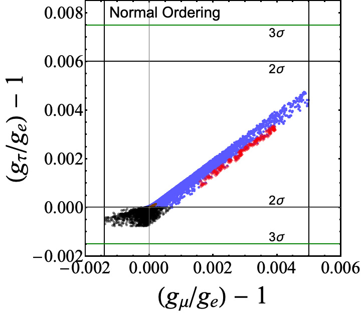
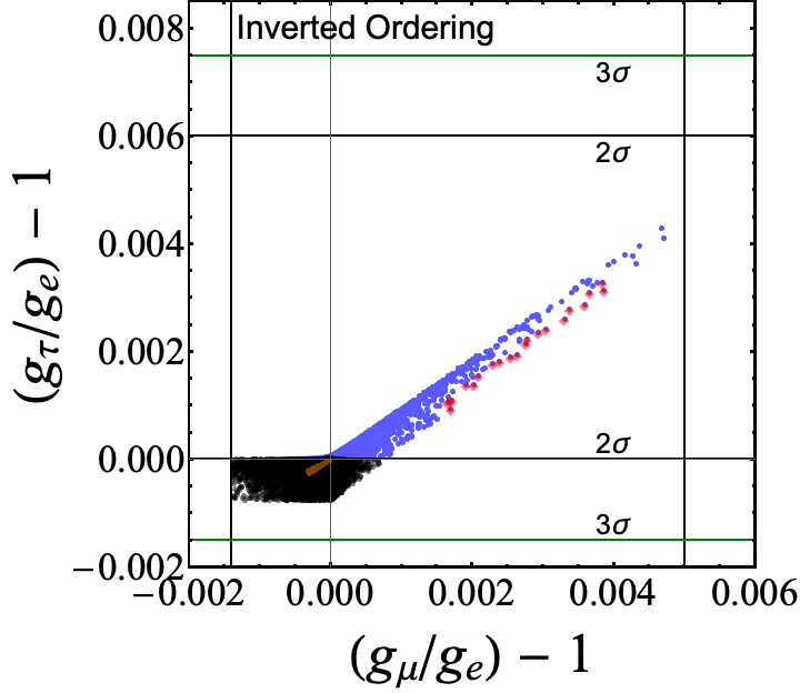
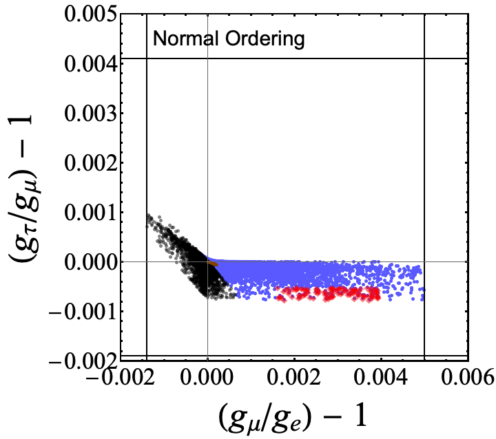
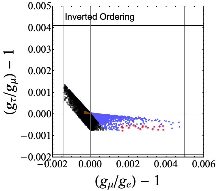
Figure 2: Correlations among deviations of $g_{\mu}/g_{e}$, $g_{\tau}/g_{e}$ (top) and $g_{\tau}/g_{\mu}$ (bottom) from universality for NO (left) and IO (right). All shown sample points explain neutrino masses and respect the bounds arising from the flavour observables considered in this work. For the blue points, the deviation of $g_{\tau}/g_{e}$ from universality is explained at $2\sigma$ in the linear case (Case I), and for the black points at $3\sigma$, but not at $2\sigma$. The red diamonds also explain the flavour anomalies, for which $g_{\tau}/g_{e}$ must be respected at $2\sigma$. Brown points pertain to the quadratic case (Case II) which only occurs at $2\sigma$ for NO and at $3\sigma$ for IO. Solid lines indicate current experimental bounds (black for $2\sigma$ or $90\text{\,}\frac{\mathrm{\char 37\relax}}{}$ CL, and green for $3\sigma$).

In the top panel of Fig. 2 we show $g_{\tau}/g_{e}-1$ as a function of $g_{\mu}/g_{e}-1$ for NO (left) and IO (right). The results of the numerical scan for the linear case are represented by blue sample points which explain $g_{\tau}/g_{e}$ at $2\sigma$, and by black sample points which explain $g_{\tau}/g_{e}$ at $3\sigma$, but not at $2\sigma$, see also the caption of Fig. 2 for details. The $3\sigma$ region for $g_{\tau}/g_{e}$ has been included to accommodate the SM prediction. If not indicated otherwise, “at $2\sigma$” and “at $3\sigma$” always refer to this distinction. Red sample points in diamond shape also explain the flavour anomalies which are briefly discussed below. The quadratic case is shown in brown. In Tab. 2 we summarise the respective confidence levels at which further experimental bounds are imposed. For the sample points, the same colour code is used throughout this work, except for Figs. 10 and 12.

We find that there are solutions to the linear-case constraint in Eq. (23) for both neutrino-mass orderings which simultaneously explain the flavour anomalies introduced above and respect the bounds from the considered flavour observables. One does in particular not have to assume that $|y^{e\tau}_{h}|$ is negligibly small. Contrariwise, explaining the flavour anomalies in the quadratic case is not possible.

In the quadratic case, no large deviations from universality can be generated. In particular, none of the respective $1\sigma$ regions for the $g_{a}/g_{b}$ which are currently preferred by experiments can be reached. Still, the corrections to both $g_{\mu}/g_{e}-1$ and $g_{\tau}/g_{e}-1$ are strictly positive (negative) for Normal (Inverted) Ordering in the quadratic case, hence a conclusive experimental determination of one of the signs would rule out one of the mass orderings being generated by $h$. Similarly, positive (negative) corrections to $g_{\tau}/g_{\mu}-1$ are severely disfavoured for NO (IO).

In the linear case, large contributions to $g_{\mu}/g_{e}$ $(g_{\tau}/g_{e})$ are disfavoured for IO as they enforce $|y^{\mu\tau}_{h}|\gg|y^{e\tau}_{h}|(|y^{e\mu}_{h}|)$, see Sect. 4.3 for more details. On the contrary, for IO we find more sample points with $g_{\tau}/g_{\mu}>1$ as shown in the bottom panel of Fig. 2. This is due to the fact that a hierarchy between $|y^{e\mu}_{h}|$ and $|y^{e\tau}_{h}|$ is easier to achieve in this case. Still, the deviation of $g_{\tau}/g_{\mu}$ from universality is measured to be smaller and an explanation of its best-fit value via $h$ would imply a further deviation from the best-fit values of the other two ratios. A given mass $M_{h}$ fixes the ranges of magnitude of $|y^{\mu\tau}_{h}|$ and $|y^{e\mu}_{h}|$ for which the flavour anomalies are explained, as in Eq. (49). Together with the strict experimental limit on $\text{Br}(\mu\to e\gamma)$ which bounds $|y^{e\tau}_{h}|$ in terms of $|y^{\mu\tau}_{h}|$, this determines the relative positions of the red and blue sample points in Fig. 2.

A more precise determination of the lepton-flavour universality ratios $g_{a}/g_{b}$ mainly relies on reducing the uncertainties in measurements of the branching ratios $\text{Br}(\tau\to\mu(e)\nu\nu)$ and of the tau lifetime Pich:2020qna . An improvement of a factor of ten is suggested in Abada:2019lih . Further improvement would rely on determining the tau mass at higher precision, for instance upon running a future tau factory at the production threshold Pich:2020qna ; Abada:2019lih ; Barniakov:2019zhx ; Luo:2019xqt . Nonetheless, shifts in the measured values $g_{a}/g_{b}$ themselves cannot be predicted and we refrain from showing estimates for prospective sensitivities in Fig. 2.

$W$-Boson Mass

The contribution to the Fermi constant induced by $h$ results in a necessarily negative correction Brivio:2017vri

$$\delta M^{2}_{W}=-\frac{M^{2}_{W}}{\sqrt{2}G_{F}}\left|1-\frac{M_{W}M_{Z}}{2M^{2}_{W}-M^{2}_{Z}}\right|\frac{|y^{e\mu}_{h}|^{2}}{M^{2}_{h}}$$ (50)

to the $W$-boson mass which exacerbates the existing $$1.5$\sigma$ tension among the SM prediction $M_{W}\pm\Delta M_{W}=$80.361\pm 0.005\text{\,}\frac{\mathrm{GeV}}{}$$ and the world average of measurements given by $M^{\text{exp}}_{W}\pm\Delta M^{\text{exp}}_{W}=$80.379\pm 0.012\text{\,}\frac{\mathrm{GeV}}{}$$ Erler:2019ddu ; Zyla:2020zbs ; Freitas:2020kcn . In order to accommodate an explanation of the flavour anomalies, we allow for a $3\sigma$ discrepancy which implies $M_{W}\geq$80.343\text{\,}\frac{\mathrm{GeV}}{}$$ and gives rise to the constraint $|y^{e\mu}_{h}|^{2}/M^{2}_{h}\lesssim$1.25$\times${10}^{-2}$/$\frac{{\mathrm{TeV}}^{2}}{}$$. To compare, the best-fit value presented in Crivellin:2020klg corresponds to $|y^{e\mu}_{h}|^{2}/M^{2}_{h}\approx$1.07$\times${10}^{-2}$/$\frac{{\mathrm{TeV}}^{2}}{}$$.

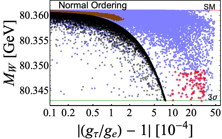
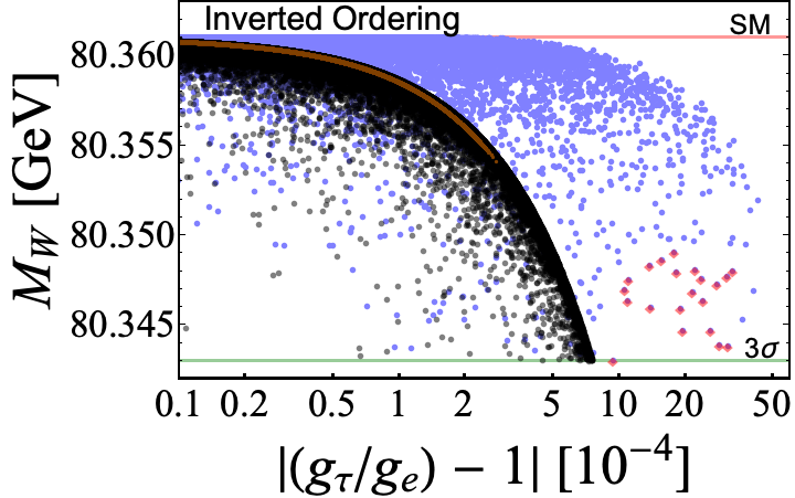
Figure 3: Correlations among $M_{W}$ and deviations of $g_{\tau}/g_{e}$ from universality. The colours are the same as in Fig. 2.

In Fig. 3 the prediction for the $W$-boson mass is shown as a function of the absolute value of the deviation of the universality ratio $g_{\tau}/g_{e}$ from one. Note that in the quadratic case the maximum correction to $M_{W}$ is much larger for IO than for NO, and there is a non-trivial correlation in the linear case especially for $|y^{e\mu}_{h}|>|y^{\mu\tau}_{h}|$. A large effect in $g_{\tau}/g_{e}-1$ together with a conclusive determination of $M_{W}$ close to its current SM prediction would severely disfavour the scenario of $h$ explaining neutrino masses with IO, but not with NO. Furthermore, a result $M_{W}\gtrsim$80.35\text{\,}\frac{\mathrm{GeV}}{}$$ would currently rule out an explanation of the flavour anomalies via $h$. In proposals for next-generation lepton colliders, a reduction of the uncertainty in the experimental determination of $M_{W}$ by a factor of roughly $10-20$ Abada:2019lih ; CEPCStudyGroup:2018ghi is suggested. As for the universality ratios $g_{a}/g_{b}$, any shifts in the obtained value $M_{W}$ itself, be it determined at colliders or via electroweak fits, cannot be predicted though.

Leptonic Non-Standard Interactions

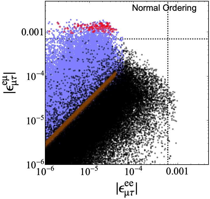
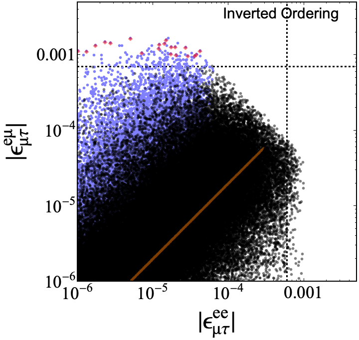
Figure 4: Non-standard interactions. The colours are the same as in Fig. 2. Dashed lines indicate prospected experimental sensitivities.

As it can be seen from Eq. (40), the singly-charged scalar singlet induces leptonic non-standard interactions at tree level, whereas NSIs with quarks only arise at loop level. Hence, we disregard the latter. The fact that the constraint in Eq. (23) disfavours large hierarchies among the coupling magnitudes (see Sect. 4.3 for more details) implies that the results found in studies in which only one NSI parameter was switched on at a time (see for instance Farzan:2017xzy ) are not directly applicable here. We obtain magnitudes of up to $|\epsilon^{\rho\sigma}_{\alpha\beta}|\sim${10}^{-3}$$ in the linear case which to our knowledge is below all current bounds and also appears to be challenging to observe in near-future experiments. For instance, depending on the flavour channel, DUNE is prospected to be sensitive to magnitudes down to $|\epsilon^{\rho\sigma}_{\alpha\beta}|\sim${10}^{-2}$$ at $90\text{\,}\frac{\mathrm{\char 37\relax}}{}$ CL Dev:2018 . Still, at a future neutrino factory it might be possible to probe some of the NSI parameters relevant for neutrino production in the $\nu_{e}\to\nu_{\tau}$ and $\nu_{\mu}\to\nu_{\tau}$ channels Herrero-Garcia:2014hfa :

$$\epsilon^{e\mu}_{\tau e} \equiv\frac{(y^{e\tau}_{h})^{*}y^{e\mu}_{h}}{\sqrt{2}G_{F}M^{2}_{h}}=-(\epsilon^{ee}_{\mu\tau})^{*}, \epsilon^{e\mu}_{\mu\tau} \equiv-\frac{(y^{e\mu}_{h})^{*}y^{\mu\tau}_{h}}{\sqrt{2}G_{F}M^{2}_{h}}\,.$$ (51)

Upon using a 2 kt OPERA-like near tau detector a sensitivity to $|\epsilon^{e\mu}_{\mu\tau}|\sim$7\text{\times}{10}^{-4}$$ and $|\epsilon^{e\mu}_{\tau e}|\sim$6\text{\times}{10}^{-4}$$ is prospected to be achievable Ohlsson:2009vk ; Tang:2009na . In that case, the simultaneous explanation of neutrino masses and the flavour anomalies via $h$ in the linear case could be conclusively tested at a neutrino factory for both neutrino-mass orderings. The contributions in the quadratic case will remain beyond reach. This is illustrated in Fig. 4. As indicated in Eq. (51), the NSI parameter $\epsilon^{e\mu}_{\tau e}$ is trivially related to the corresponding one for the propagation of $\nu_{\mu}$ and $\nu_{\tau}$ neutrinos in matter.

4.2 Charged Lepton Flavour Violation

The leading-order contributions to flavour-violating charged-lepton decays from singly-charged scalar singlets occur at one-loop level. In fact, finite contributions to radiative charged-lepton decays $\ell_{i}\to\ell_{j}\gamma$ are sourced by a single diagram with a neutrino $\nu_{k}$, $i\neq j$ and $i\neq k\neq j$, in the loop. The branching ratios are given by PETCOV1982401 ; Nebot:2007bc ; BERTOLINI1988714 ; RevModPhys.59.671 ; PICH1984229 ; Crivellin:2020klg

$$\text{Br}(\mu\to e\gamma) =\text{Br}(\mu\to e\nu\bar{\nu})\frac{\alpha_{\text{EM}}}{48\pi G^{2}_{F}}\frac{|y^{e\tau}_{h}y^{\mu\tau}_{h}|^{2}}{M^{4}_{h}},$$ (52)

$$\text{Br}(\tau\to e\gamma) =\text{Br}(\tau\to e\nu\bar{\nu})\frac{\alpha_{\text{EM}}}{48\pi G^{2}_{F}}\frac{|y^{e\mu}_{h}y^{\mu\tau}_{h}|^{2}}{M^{4}_{h}},$$ (53)

$$\text{Br}(\tau\to\mu\gamma) =\text{Br}(\tau\to\mu\nu\bar{\nu})\frac{\alpha_{\text{EM}}}{48\pi G^{2}_{F}}\frac{|y^{e\mu}_{h}y^{e\tau}_{h}|^{2}}{M^{4}_{h}}\,,$$ (54)

with $\text{Br}(\mu\to e\nu\bar{\nu})\approx 1$, $\text{Br}(\tau\to e\nu\bar{\nu})\approx$0.178$$ and $\text{Br}(\tau\to\mu\nu\bar{\nu})\approx$0.174$$ Zyla:2020zbs . As it can be seen in Fig. 5, any signal in radiative tau decays showing up at Belle II cannot be induced by $h$ alone, see Table 2. For instance, one would need two singly-charged scalar singlets which conspire to circumvent the strong bounds arising from flavour-violating muon decays.

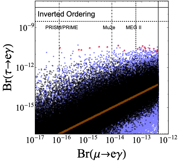
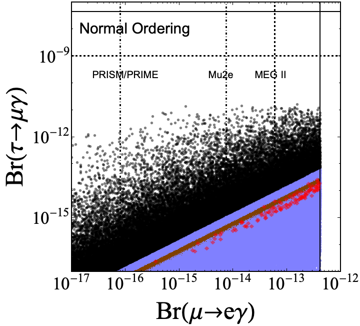
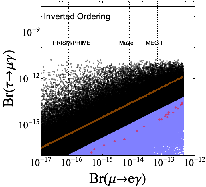
Figure 5: Branching ratios of radiative charged-lepton decays. The vertical dot-dashed lines correspond to the prospected sensitivities to $\text{Br}(\mu\to e\text{;}\;\text{Ti})$ at PRISM/PRIME and to $\text{Br}(\mu\to e\text{;}\;\text{Al})$ at Mu2e which were then converted via $\text{Br}(\mu\to e\text{;}\;\text{Al})\approx$0.0079$\,\text{Br}(\mu\to e\gamma)$ and $\text{Br}(\mu\to e\text{;}\;\text{Ti})\approx$0.0125$\,\text{Br}(\mu\to e\gamma)$, see also App. C. The colours are the same as in Fig. 2.

Also the sizeable contributions to $\tau\to e\gamma$ implied by simultaneously generating neutrino mass and explaining the flavour anomalies will be beyond reach Crivellin:2020klg . Instead, a future search for $\mu\to e\gamma$ Baldini:2018nnn efficiently probes parts of the parameter space pertaining to $h$ generating neutrino masses both in the linear case and in the quadratic case, as well as the combined scenario in which also the flavour anomalies are explained in the linear case.

As it is well-known, if the contributions from on-shell photon penguin diagrams dominate, the branching ratios for tri-lepton decays with only one flavour in the final state are entirely fixed as functions of $\text{Br}(\ell_{i}\to\ell_{j}\gamma)$ and SM parameters: Kuno:1999jp ; Crivellin:2013hpa

$$\frac{\text{Br}(\mu\to 3e)}{\text{Br}(\mu\to e\gamma)} \approx\frac{\alpha_{\text{EM}}}{3\pi}\left(\log\left(\frac{m^{2}_{\mu}}{m^{2}_{e}}\right)-\frac{11}{4}\right)\approx\frac{1}{163},$$ (55)

$$\frac{\text{Br}(\tau\to 3e)}{\text{Br}(\tau\to e\gamma)} \approx\frac{\alpha_{\text{EM}}}{3\pi}\left(\log\left(\frac{m^{2}_{\tau}}{m^{2}_{e}}\right)-\frac{11}{4}\right)\approx\frac{1}{95},$$ (56)

$$\frac{\text{Br}(\tau\to 3\mu)}{\text{Br}(\tau\to\mu\gamma)} \approx\frac{\alpha_{\text{EM}}}{3\pi}\left(\log\left(\frac{m^{2}_{\tau}}{m^{2}_{\mu}}\right)-\frac{11}{4}\right)\approx\frac{1}{446}\,.$$ (57)

For masses close to the lower bound $M_{h}=$350\text{\,}\frac{\mathrm{GeV}}{}$$, the photon-penguin approximation is perfectly valid. In the quadratic case, the relative magnitudes of the couplings $y^{ij}_{h}$ are quite sensitive to the neutrino-mass ordering, as dictated in Eq. (29). Together with the flavour-dependent suppression factors $\sim\log(m_{k}/m_{l})$, this efficiently determines the relative size of the different radiative charged-lepton decay channels in the photon-penguin limit. On the contrary, note how the contributions from box diagrams outperform those from photon penguins for $\tau\to 3\mu$ in the case of NO, as can be seen in Fig. 6.

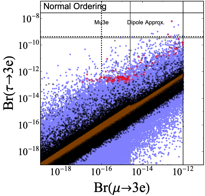
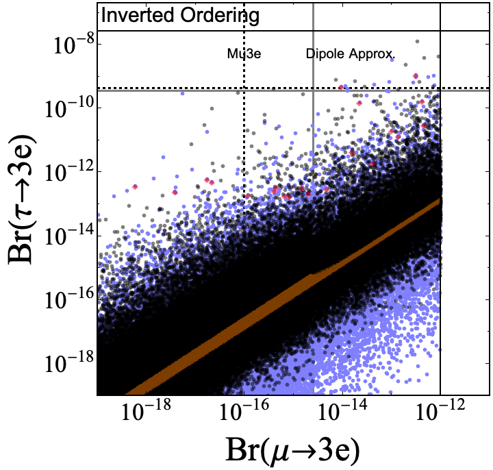
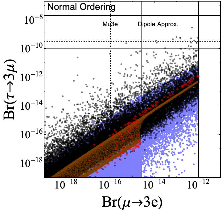
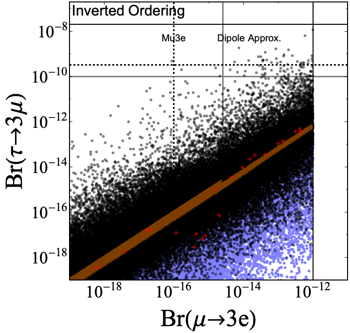
Figure 6: Branching ratios of tri-lepton decays. The colours are the same as in Fig. 2. The solid grey lines indicate the respective experimental bounds that would apply to the photon-penguin approximation. Dashed lines indicate prospected experimental sensitivities.

The vertical solid grey lines in Fig. 6 indicate the bound induced by $\mu\to e\gamma$ which is the relevant one both for the linear case and for the quadratic case as long as the photon penguin dominates $\mu\to 3e$. In the numerical scan, the full expression as given in Crivellin:2020klg is used, because larger masses $M_{h}$ generally render larger magnitudes $|y^{ij}_{h}|$ compatible with the different experimental bounds, which in turn implies that the contributions from box diagrams to tri-lepton decays become increasingly dominant. Since box diagrams are proportional to the product of four Yukawa couplings, they can thus induce contributions to tri-lepton decays which in fact grow if the mass increases beyond $M_{h}\approx$1\text{\,}\frac{\mathrm{TeV}}{}$$ and further. Thus, $h$ will decouple from the phenomenology at low energy only for even larger masses $M_{h}\gg$100\text{\,}\frac{\mathrm{TeV}}{}$$. This is distinctively visible in Fig. 7 where we show $\tau\to 3e(\mu)$ as a function of the singly-charged scalar singlet mass $M_{h}$.

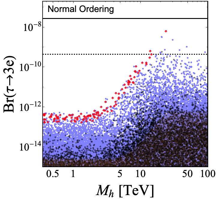
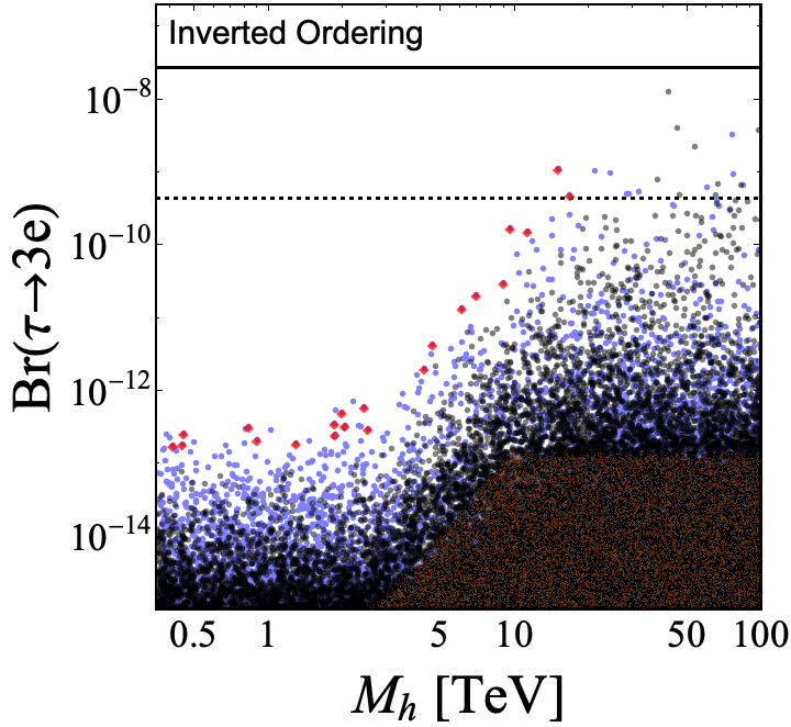
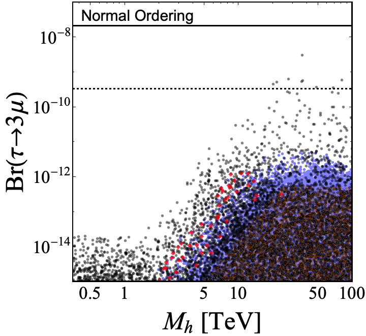
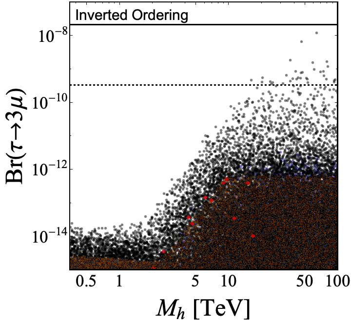
Figure 7: Branching ratio of tri-lepton tau decays as a function of the mass $M_{h}$. The colours are the same as in Fig. 2. Dashed lines indicate prospected experimental sensitivities.

As the figures illustrate, masses larger than $M_{h}\gtrsim$11\text{\,}\frac{\mathrm{TeV}}{}$$ and $M_{h}\gtrsim$15\text{\,}\frac{\mathrm{TeV}}{}$$ can induce an observable signal in $\tau\to 3e$ and $\tau\to 3\mu$, respectively, at Belle II Kou:2018nap .

Besides $\mu\to 3e$ Arndt:2020obb which will be sensitive both to the linear case and the quadratic case, tri-lepton tau decay thus offer another avenue for testing the generation of neutrino masses via $h$ at larger masses $M_{h}$ in the linear case, complementary to $\mu\to e\gamma$ for which the contributions start to decrease before the assumed upper limit $M_{h}\leq$100\text{\,}\frac{\mathrm{TeV}}{}$$ is reached. Via $\tau\to 3e$ we are even sensitive to parts of the parameter space for which the flavour anomalies are explained as well Crivellin:2020klg . Still, the constraint in Eq. (23) disfavours the solutions $y^{ij}_{h}$ which induce large contributions to $\tau\to 3e(\mu)$ as there needs to be a hierarchy among the coupling magnitudes $|y^{e\mu}_{h}|$ and $|y^{\mu\tau}_{h}|$ ($|y^{e\tau}_{h}|$) entering the relevant box diagram and $|y^{e\tau}_{h}|$ ($|y^{\mu\tau}_{h}|$) which must be smaller in order not to violate the experimental bound on $\text{Br}(\mu\to e\gamma)$.

A further relevant process is $\mu-e$ conversion in nuclei which probes the same parameter combination as $\mu\to e\gamma$ and is dominated by photon-penguin diagrams. As of today, the strongest constraint arises from the SINDRUM-II experiment in which a gold target was used Bertl:2006up . Taking into account both the short-range and the long-range contribution (see App. C), one finds $\text{Br}(\mu\to e\text{;}\;\text{Au})\equiv\omega^{\text{Au}}_{\text{conv}}/\omega^{\text{Au}}_{\text{capt}}\approx$0.0130$\;\text{Br}(\mu\to e\gamma)$ for $\mu-e$ conversion in gold Crivellin:2018qmi ; Kitano:2002mt ; Crivellin:2020klg . Hence, the process does not yield a competitive constraint yet, still, in the photon-penguin approximation it is less suppressed with respect to $\mu\to e\gamma$ than $\mu\to 3e$. In addition, future experiments on $\mu-e$ conversion are prospected to outperform current and future searches for radiative charged-lepton decays in sensitivity by far Kutschke:2011ux ; Hungerford:2009zz ; Kuno:2005mm . For instance, PRISM/PRIME can be expected to almost conclusively test the simultaneous explanation of neutrino masses and the flavour anomalies.

As a side note, the singly-charged scalar singlet also generates contributions to anomalous magnetic moments. However, the contribution is always negative Nebot:2007bc ; 1985PhRvD..31..105M ; LEVEILLE197863 ; Lindner:2016bgg , hence it is not possible to explain the long-standing anomaly $\delta a_{\mu}\equiv a^{\text{exp}}_{\mu}-a^{\text{SM}}_{\mu}=(2.51\pm 0.59)\times 10^{-9}$ Bennett:2006fi ; Aoyama:2020ynm ; Abi:2021gix . We find contributions to the anomalous magnetic moment of the muon of up to $\delta a_{\mu}\approx$-{10}^{-11}$$. Similarly, in the electron case, the contribution $\delta a_{e}\approx$-{10}^{-16}$$ is small compared to the experimental uncertainty which is of order ${10}^{-13}$ Hanneke:2008tm ; Hanneke:2010au ; Parker:2018vye ; Morel:2020dww .

4.3 Magnitude of Couplings

The constraint in Eq. (23) tends to correlate the couplings $y^{ij}_{h}$ in such a way that in many cases at least two of them are comparable in magnitude, as it can be seen in Fig. 8.

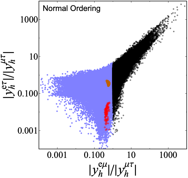
Figure 8: Plot of the coupling ratios $|y^{e\mu}_{h}|/|y^{\mu\tau}_{h}|$ and $|y^{e\tau}_{h}|/|y^{\mu\tau}_{h}|$ as obtained in the numerical scan. The colours are the same as in Fig. 2.

.

We show the ratios because the magnitudes $|y^{ij}_{h}|$ of the elements of $v_{h}$ in Eq. (23) can always be rescaled by a common factor and hence only the relative magnitudes are determined via the constraint. It is distinctively visible how viable parameter space opens up upon replacing the condition in Eq. (29) by the more general one in Eq. (23).

For NO, solutions with $|y^{\mu\tau}_{h}|$ larger than both $|y^{ei}_{h}|$, $i=\mu,\tau$ are most abundant and in particular the hierarchies $|y^{e\mu}_{h}|<|y^{\mu\tau}_{h}|<|y^{e\tau}_{h}|$ and $|y^{e\tau}_{h}|<|y^{\mu\tau}_{h}|<|y^{e\mu}_{h}|$ are rather disfavoured, hence, there is a tendency for $|y^{\mu\tau}_{h}|\gtrsim|y^{e\mu}_{h}|\approx|y^{e\tau}_{h}|$. On the contrary, for IO there are smaller differences in how often the different hierarchies are obtained. Note that while the viable regions in parameter space in Fig. 8 do in general not feature a sharp contour, the most distinctive deviation from that tendency occurs if both $|y^{e\mu}_{h}|/|y^{\mu\tau}_{h}|\lesssim$0.1$$ and $|y^{e\tau}_{h}|/|y^{\mu\tau}_{h}|\lesssim$0.1$$ for which viable solutions seem to be rigorously excluded in the case of IO. Hence, if the coupling $y^{\mu\tau}_{h}$ was experimentally confirmed to sufficiently dominate over the electron-flavoured ones in magnitude, this would appear to leave us only with the possibility of $h$ generating the main contribution to neutrino masses with NO. The corresponding experimental signature would be a vanishingly small branching ratio for the decay channel $h\to e\nu$, see also Sect. 4.4.

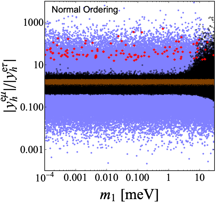
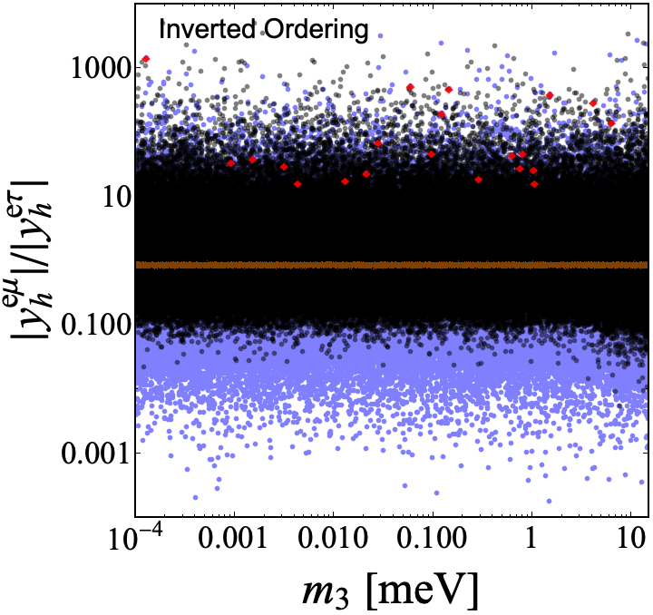
Figure 9: Plot of the coupling ratios $|y^{e\mu}_{h}|/|y^{e\tau}_{h}|$ as a function of the smallest neutrino mass ($m_{1}$ for NO, and $m_{3}$ for IO). The colours are the same as in Fig. 2.

Besides, as it can be seen in Fig. 9, if $|y^{e\mu}_{h}|>|y^{\mu\tau}_{h}|$, which corresponds to black sample points, the constraint in Eq. (23) further disfavours solutions with $|y^{e\mu}_{h}|/|y^{e\tau}_{h}|\lesssim$0.1$$. In addition, if the lightest neutrino is not much heavier than $m_{0}=m_{1}\approx$1\text{\,}\frac{\mathrm{meV}}{}$$ in the case of NO, $|y^{e\mu}_{h}|>|y^{\mu\tau}_{h}|$ is only viable for $|y^{e\mu}_{h}|/|y^{e\tau}_{h}|\lesssim$10$$. We trace this back to the fact that for NO the neutrino mass matrix is known to feature a slight hierarchy between the magnitudes of the components in the first row (and column) and those in the 23-block, which only diminishes if the smallest neutrino mass $m_{1}$ becomes large.

Of course, these solutions are not obtained if one solves the constraint in Eq. (23) with the additional condition of one Majorana phase and the smallest neutrino mass vanishing. Still, there are no major differences in the obtained phenomenology compared to the general case with three massive neutrinos. In particular, one does not enjoy the same predictive power as in the quadratic case for which the smallest neutrino mass vanishes, $m_{0}=0$, automatically. On the contrary, for IO the $|M^{ij}_{\nu}|$ are more similar in magnitude and less sensitive to $m_{3}$, and thus so are the $|y^{ij}_{h}|$.

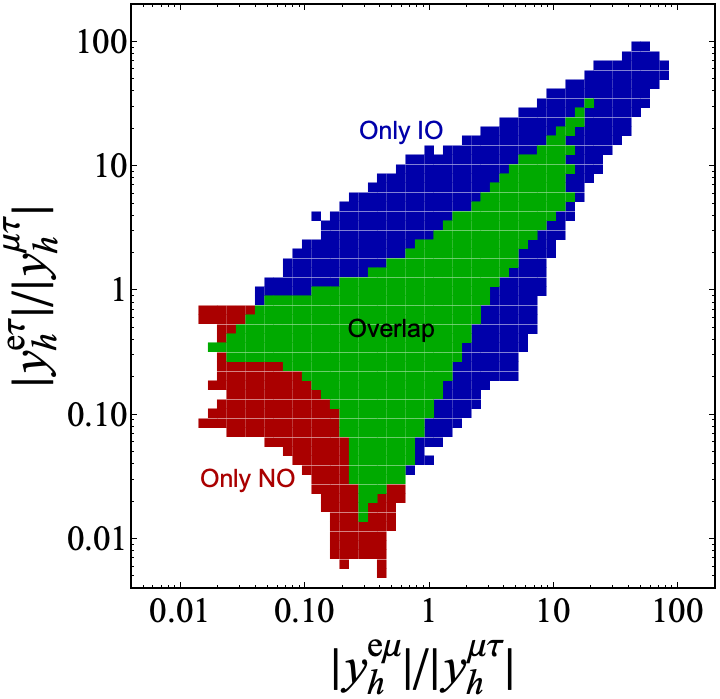
Figure 10: Plot of the coupling ratios $|y^{e\mu}_{h}|/|y^{\mu\tau}_{h}|$ and $|y^{e\tau}_{h}|/|y^{\mu\tau}_{h}|$ as obtained in the numerical scan if approximately $95.45\text{\,}\frac{\mathrm{\char 37\relax}}{}$ of the overall number of $547991$ ($542287$) sample points generated for NO (IO) are taken into account. Each square shown to be compatible with NO (IO) contains at least 97 (74) sample points. See also main text.

Furthermore, a determination of the relative size of the regions in the parameter space of coupling magnitudes which are compatible only with NO or with IO, or with both is performed. The strategy is to discretise the parameter space into a grid structure and to count the sample points contained in each grid square, starting with the square containing the largest number of points and then gradually moving on to those with fewer points, until a specified portion of the overall number of sample points is taken into account. Fig. 10 shows the region of approximately $95.45\text{\,}\frac{\mathrm{\char 37\relax}}{}$ of the sample points.

4.4 Decay Channels of the Singly-Charged Scalar Singlet

The partial width of the decay of a singly-charged scalar singlet into a charged lepton $\ell$ and a neutrino $\nu$ is given by Nebot:2007bc

$$\Gamma(h\to\ell_{a}\nu_{b})=\Gamma(h\to\ell_{b}\nu_{a})=\frac{|y^{ab}_{h}|^{2}}{4\pi}M_{h}\,.$$ (58)

Leaving the undetected neutrino flavour unspecified, one obtains the branching ratio for the decay of $h$ into a charged lepton of flavour $a$ and a neutrino:

$$\text{Br}(h\to\ell_{a}\nu)=\frac{\sum_{b\neq a}|y^{ab}_{h}|^{2}}{2(|y_{h}^{e\mu}|^{2}+|y_{h}^{e\tau}|^{2}+|y_{h}^{\mu\tau}|^{2})}\,.$$ (59)

Regardless of whether the magnitudes $|y^{ij}_{h}|$ are constrained in some way or not, the individual branching ratios always take a value between 0 and $0.5$.

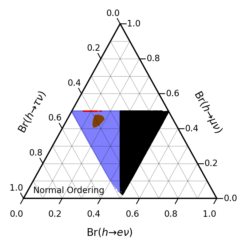
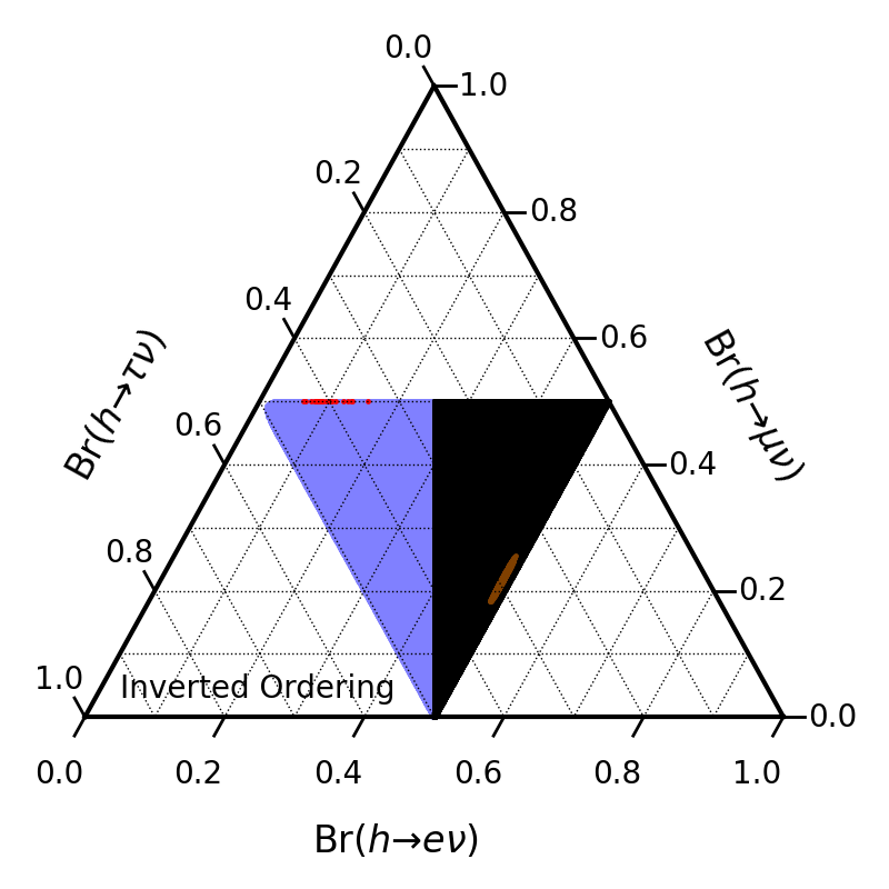
Figure 11: Branching ratios of $h\to\ell\nu$. The colours are the same as in Fig. 2.

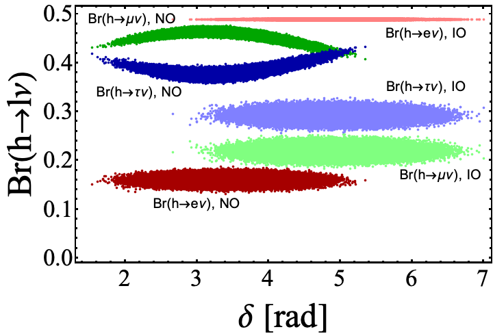
Figure 12: Branching ratios of the different channels $h\to\ell\nu$ as functions of the Dirac CP phase $\delta$ in the quadratic case (Case II).

A very small or vanishing branching ratio for the electron channel (and consequently $\text{Br}(h\to\mu\nu)\approx\text{Br}(h\to\tau\nu)\approx$0.5$$) is supported in NO, but severely disfavoured for IO, as it can be seen in Fig. 11. Contrariwise, obtaining a (near-)maximal branching to taus and a small one to muons is disfavoured by NO, but compatible with IO. For the more restrictive constraint in Eq. (29), the muon and tau channels exhibit a slight correlation with the CP-violating phase $\delta$ in the case of NO which is illustrated in Fig. 12 and has been discussed before in Herrero-Garcia:2014hfa for the Zee-Babu model. It is due to the fact that for IO $\delta$ only fixes the phases $\arg(y^{ei}_{h})$, while it also determines $|y^{\mu\tau}_{h}|$ in the case of NO.

5 Multiple Singly-Charged Scalar Singlets

Lastly, we comment on the possibility of generating $1,...,n$ sizeable contributions to neutrino masses via multiple singly-charged scalar singlets $h_{1},...,h_{n}$ and focus on $n=2$ for simplicity.

The overall lepton sector for two singly-charged singlet scalars is given by

$$\mathcal{L}_{\text{lept}}=y^{ij}_{e}\bar{e}_{i}L_{j}H^{*}+y^{ij}_{h_{1}}L_{i}L_{j}h_{1}+y^{ij}_{h_{2}}L_{i}L_{j}h_{2}+\text{h.c.}.$$ (60)

We again can distinguish the linear and the quadratic case and focus on the latter first. We assume that the main contribution to neutrino masses consists of diagrams in which both external neutrinos couple to the respective loop structure via $y_{h_{1}}$ or $y_{h_{2}}$. Then, the most general neutrino mass matrix reads

$$U^{*}m_{\text{diag}}U^{\dagger}=M_{\nu}=y^{T}_{h_{1}}S_{1}y_{h_{1}}+y^{T}_{h_{2}}S_{2}y_{h_{2}}+y^{T}_{h_{1}}Zy_{h_{2}}+y^{T}_{h_{2}}Z^{T}y_{h_{1}}\,,$$ (61)

with the symmetric coupling matrices $S_{1,2}$ and a general matrix $Z$. Multiplying Eq. (61) by the respective eigenvectors $v_{h_{1,2}}$ of $y_{h_{1,2}}$ with eigenvalue zero, one obtains three inequivalent complex conditions:

$$v^{T}_{h_{1}}U^{*}m_{\text{diag}}U^{\dagger}v_{h_{1}} =v^{T}_{h_{1}}y^{T}_{h_{2}}S_{2}y_{h_{2}}v_{h_{1}},$$ (62a)

$$v^{T}_{h_{2}}U^{*}m_{\text{diag}}U^{\dagger}v_{h_{1}} =v^{T}_{h_{2}}y^{T}_{h_{1}}Zy_{h_{2}}v_{h_{1}},$$ (62b)

$$v^{T}_{h_{2}}U^{*}m_{\text{diag}}U^{\dagger}v_{h_{2}} =v^{T}_{h_{2}}y^{T}_{h_{1}}S_{1}y_{h_{1}}v_{h_{2}}\,.$$ (62c)

Contrary to the linear case and the quadratic case discussed for one singly-charged scalar singlet before, here the constraint explicitly involves the matrices $S_{1,2}$ and $Z$ which parametrise the breaking of lepton-number conservation. In that sense, Eqs. (62a)-(62c) are in general model-dependent and hence less predictive. In App. D we present one possible neutrino mass model with two singly-charged scalar singlets as an example.

In explicit models, some of the matrices $S_{1,2},Z$ may vanish in the case of an additional symmetry. Then, the respective expressions above would simplify accordingly and one could solve them as in the linear case. Still, irrespective of the specific structures in $S_{1,2}$ and $Z$, all Eqs. (62a)-(62c) have to be individually satisfied. Thus, the contributions $y^{T}_{h_{1}}S_{1}y_{h_{1}}$ and $y^{T}_{h_{2}}S_{2}y_{h_{2}}$ are not independent, but the elements of $y_{h_{1}}$ and $y_{h_{2}}$ are intertwined via each of the right-hand sides and in particular also via the left-hand side of Eq. (62b) even if $Z$ is taken to zero. Only if both $Z$ and one of the matrices $S_{1}$ and $S_{2}$ are absent, one trivially recovers the quadratic case for one singly-charged scalar singlet. The same limit is obtained for a large hierarchy between the masses of $h_{1}$ and $h_{2}$ since one may integrate out the heavier singlet and attain more predictive power. Lastly, it is straightforward to generalise Eq. (61) towards the case of $n$ singly-charged scalar singlets generating sizeable contributions to neutrino masses.

In the linear case, one would generalise the structure of the neutrino mass matrix towards

$$U^{*}m_{\text{diag}}U^{\dagger}=M_{\nu}=X_{1}y_{h_{1}}-y_{h_{1}}X_{1}^{T}+X_{2}y_{h_{2}}-y_{h_{2}}X_{2}^{T}\,.$$ (63)

Still, there is no non-trivial limit in which the derived constraints would become independent of the model-dependent physics in $X_{1,2}$.

6 Conclusions

We have presented a classification and phenomenological study for scenarios in which a singly-charged scalar singlet particle $h$ generates the main contribution to neutrino masses. Among the SM fermions, $h$ interacts only with the left-handed lepton doublets via an antisymmetric Yukawa coupling $y_{h}LLh+\text{h.c.}$ at tree level. It is possible to assign charges of lepton number to $h$ and the SM leptons in a way such that it is respected by all renormalisable terms in the Lagrangian. Thus, in order to generate Majorana masses for neutrinos, one needs to introduce a source of lepton-number breaking. Our approach is independent of the details of this breaking. The only assumption is that the main contribution of neutrino masses is generated by a diagram in which one or both of the external neutrinos couples via $y_{h}$.

For the minimal case of just one singlet state, this gives rise to only two possible structures for the neutrino mass matrix. Regarding the Feynman diagram which generates the main contribution to neutrino masses, we distinguish between the “linear case” in which only one external neutrino is linked to the loop structure via $y_{h}$, and the “quadratic case” in which both external neutrinos are. Several well-known models of neutrino-mass generation fall into those two categories: The Zee model Zee:1980ai ; Cheng:1980qt ; WOLFENSTEIN198093 is an example for the linear case and the Zee-Babu Zee:1985id ; Zee:1985rj ; Babu:1988ki and KNT models Krauss:2002px are examples for the quadratic case.

For each of the cases, we employ the antisymmetry of $y_{h}$ in flavour space to derive a model-independent constraint which has to be satisfied to guarantee the correct description of the measured mixing and mass hierarchy of neutrinos. In the linear case, the constraint determines two of the magnitudes of the Yukawa coupling matrix elements $|y_{h}^{ij}|$ in terms of the third one, the two phases of $y_{h}^{ei}$, $i=\mu,\tau$, neutrino masses, leptonic mixing angles and phases. In the quadratic case, the two constraints are independent of the neutrino masses and Majorana phases and thus more predictive.

This enables us to perform a phenomenological study applicable to many different types of models. The study is conservative in the sense that no other contributions to the considered observables beyond the ones induced by $h$ are taken into account. If the other new particles involved in a specific model are sufficiently decoupled in the sense that they are very heavy or very weakly coupled to the SM, the phenomenological bounds obtained will approximately coincide with those of the actual model, otherwise the bounds will be weaker. This is trivially satisfied in an effective field theory framework, in which the singly-charged scalar singlet is much lighter than all other new particles.

For the linear case, the constraint disfavours large hierarchies among the coupling magnitudes $y^{ij}_{h}$ and hence the available parameter space is mostly shaped by $\mu\to e\gamma$ and $\mu\to 3e$ and other low-energy processes are generally not competitive. The relative magnitudes $|y^{ij}_{h}|$ display some sensitivity to the neutrino-mass ordering. Furthermore, we demonstrate that the region in parameter space where the Cabibbo Angle Anomaly and the deviation of leptonic gauge couplings from universality, collectively dubbed the “flavour anomalies”, are explained by $h$ is compatible with, albeit not preferred by neutrino masses. A conclusive measurement of $M_{W}>$80.35\text{\,}\frac{\mathrm{GeV}}{}$$ would imply that $h$ cannot explain the flavour anomalies.

For the quadratic case, the parameter space is strongly constrained by neutrino masses and thus the scenario is very predictive. The leptonic gauge couplings do not receive large contributions and thus it is not possible to explain their deviation from universality as indicated by current data and neither the Cabibbo Angle Anomaly. Furthermore, there is a tight correlation between the different radiative charged-lepton decays and hence any signal of a radiative flavour-violating tau decay at Belle II would imply that low-energy effects of new physics cannot be assumed to be dominated by $h$. Also, one may derive sharp predictions for the branching ratios of the different decay channels to satisfy $\text{Br}(h\to\tau\nu)\simeq\text{Br}(h\to\mu\nu)\sim$0.4$$ and $\text{Br}(h\to e\nu)\lesssim$0.2$$ for NO and $\text{Br}(h\to\tau\nu)\sim$0.3$$, $\text{Br}(h\to\mu\nu)\sim$0.2$$ and $\text{Br}(h\to e\nu)\sim 0.5$ for IO. The branching ratios $\text{Br}(h\to\tau\nu)$ and $\text{Br}(h\to\mu\nu$) exhibit a slight dependence on the Dirac CP phase $\delta$ for NO.

Finally, we commented on the generalisation of our framework to multiple singly-charged scalar singlets. One may also derive constraints in that case, but they depend on the breaking of lepton number and thus do not allow for a model-independent study.

To conclude, this study of the singly-charged scalar singlet $h$ is a neat example of a model-independent approach towards neutrino masses and their phenomenological implications. The constraints originate only from the form of the neutrino mass matrix and the antisymmetry of the Yukawa coupling of $h$ to left-handed lepton doublets. We leave the discussion of other simplified neutrino mass scenarios for future work.

Appendix A Neutrino-Mass Constraint Spelt in Full

Written out, the constraint in Eq. (23) explicitly reads

$$\Bigg{(}\Big{(}c_{13}^{2}m_{3}c_{23}^{2}+e^{-2i\eta_{2}}m_{2}\left(e^{-i\delta}c_{23}s_{12}s_{13}+c_{12}s_{23}\right)^{2}+$$ (64)

$$e^{-2i\eta_{1}}m_{1}\left(e^{-i\delta}c_{12}c_{23}s_{13}-s_{12}s_{23}\right)^{2}\Big{)}y_{h}^{\text{e$\mu$}}$$

$$- \Big{(}c_{23}m_{3}s_{23}c_{13}^{2}+e^{-2i\eta_{1}}m_{1}\left(e^{-i\delta}c_{12}c_{23}s_{13}-s_{12}s_{23}\right)\left(c_{23}s_{12}+e^{-i\delta}c_{12}s_{13}s_{23}\right)$$

$$- e^{-2i\eta_{2}}m_{2}\left(e^{-i\delta}c_{23}s_{12}s_{13}+c_{12}s_{23}\right)\left(c_{12}c_{23}-e^{-i\delta}s_{12}s_{13}s_{23}\right)\Big{)}y_{h}^{\text{e$\tau$}}$$

$$+ c_{13}\Big{(}e^{i\delta}c_{23}m_{3}s_{13}-e^{-2i\eta_{2}}m_{2}s_{12}\left(e^{-i\delta}c_{23}s_{12}s_{13}+c_{12}s_{23}\right)$$

$$+ e^{-2i\eta_{1}}c_{12}m_{1}\left(s_{12}s_{23}-e^{-i\delta}c_{12}c_{23}s_{13}\right)\Big{)}y_{h}^{\mu\tau}\Bigg{)}y_{h}^{\text{e$\mu$}}$$

$$- \Bigg{(}\Big{(}c_{23}m_{3}s_{23}c_{13}^{2}+e^{-2i\eta_{1}}m_{1}\left(e^{-i\delta}c_{12}c_{23}s_{13}-s_{12}s_{23}\right)\left(c_{23}s_{12}+e^{-i\delta}c_{12}s_{13}s_{23}\right)$$

$$- e^{-2i\eta_{2}}m_{2}\left(e^{-i\delta}c_{23}s_{12}s_{13}+c_{12}s_{23}\right)\left(c_{12}c_{23}-e^{-i\delta}s_{12}s_{13}s_{23}\right)\Big{)}y_{h}^{\text{e$\mu$}}$$

$$- \Big{(}c_{13}^{2}m_{3}s_{23}^{2}+e^{-2i\eta_{1}}m_{1}\left(c_{23}s_{12}+e^{-i\delta}c_{12}s_{13}s_{23}\right)^{2}$$

$$+e^{-2i\eta_{2}}m_{2}\left(c_{12}c_{23}-e^{-i\delta}s_{12}s_{13}s_{23}\right)^{2}\Big{)}y_{h}^{\text{e$\tau$}}$$

$$- e^{i\delta}c_{13}\Big{(}e^{-2i\left(\delta+\eta_{1}\right)}m_{1}s_{13}s_{23}c_{12}^{2}+e^{-i\delta}c_{23}\left(e^{-2i\eta_{1}}m_{1}-e^{-2i\eta_{2}}m_{2}\right)s_{12}c_{12}$$

$$- \left(m_{3}-e^{-2i\left(\delta+\eta_{2}\right)}m_{2}s_{12}^{2}\right)s_{13}s_{23}\Big{)}y_{h}^{\mu\tau}\Bigg{)}y_{h}^{\text{e$\tau$}}$$

$$+ \Bigg{(}c_{13}\Big{(}e^{i\delta}c_{23}m_{3}s_{13}-e^{-2i\eta_{2}}m_{2}s_{12}\left(e^{-i\delta}c_{23}s_{12}s_{13}+c_{12}s_{23}\right)$$

$$+ e^{-2i\eta_{1}}c_{12}m_{1}\left(s_{12}s_{23}-e^{-i\delta}c_{12}c_{23}s_{13}\right)\Big{)}y_{h}^{\text{e$\mu$}}$$

$$+ e^{i\delta}c_{13}\Big{(}e^{-2i\left(\delta+\eta_{1}\right)}m_{1}s_{13}s_{23}c_{12}^{2}+e^{-i\delta}c_{23}\left(e^{-2i\eta_{1}}m_{1}-e^{-2i\eta_{2}}m_{2}\right)s_{12}c_{12}$$

$$- \left(m_{3}-e^{-2i\left(\delta+\eta_{2}\right)}m_{2}s_{12}^{2}\right)s_{13}s_{23}\Big{)}y_{h}^{\text{e$\tau$}}$$

$$+ \left(e^{-2i\eta_{2}}m_{2}s_{12}^{2}c_{13}^{2}+e^{-2i\eta_{1}}c_{12}^{2}m_{1}c_{13}^{2}+e^{2i\delta}m_{3}s_{13}^{2}\right)y_{h}^{\mu\tau}\Bigg{)}y_{h}^{\mu\tau}=0\,,$$

with the abbreviations $s_{ij}\equiv\sin(\theta_{ij})$ and $c_{ij}\equiv\cos(\theta_{ij})$.

Appendix B Effective Four-Lepton Operator

Starting from the full theory as defined via Eqs. (1) and (2), one obtains the lowest-order solution to the classical equation of motion for $h$:

$$h=-\frac{(y^{ij}_{h})^{*}}{M^{2}_{h}}L^{\dagger}_{j}L^{\dagger}_{i}\,.$$ (65)

The resulting effective Lagrangian reads

$$\mathcal{L}_{\text{eff}}=\frac{(y^{ij}_{h})^{*}y^{kl}_{h}}{M^{2}_{h}}L^{\dagger}_{j}L^{\dagger}_{i}L_{k}L_{l}=\frac{(y^{ik}_{h})^{*}y^{jl}_{h}}{M^{2}_{h}}L^{\dagger\alpha}_{i}\bar{\sigma}^{\mu}L_{j\alpha}L^{\dagger\beta}_{k}\bar{\sigma}_{\mu}L_{l\beta}.$$ (66)

In order to derive this result, one first observes that

$$L^{\dagger}_{j}L^{\dagger}_{i}L_{k}L_{l}=L^{\dagger\alpha}_{j}L^{\dagger\beta}_{i}L_{k\beta}L_{l\alpha}-L^{\dagger\alpha}_{j}L^{\dagger\beta}_{i}L_{k\alpha}L_{l\beta}.$$ (67)

Together with the antisymmetry of $y_{h}$, this implies

$$\frac{(y^{ij}_{h})^{*}y^{kl}_{h}}{M^{2}_{h}}L^{\dagger}_{j}L^{\dagger}_{i}L_{k}L_{l}=2\frac{(y^{ij}_{h})^{*}y^{kl}_{h}}{M^{2}_{h}}L^{\dagger\alpha}_{j}L^{\dagger\beta}_{i}L_{k\beta}L_{l\alpha}.$$ (68)

Then, applying a Fierz transformation and relabeling flavour indices yields the result

$$\frac{(y^{ij}_{h})^{*}y^{kl}_{h}}{M^{2}_{h}}L^{\dagger}_{j}L^{\dagger}_{i}L_{k}L_{l} =\frac{(y^{ij}_{h})^{*}y^{kl}_{h}}{M^{2}_{h}}L^{\dagger\alpha}_{j}\bar{\sigma}^{\mu}L_{l\alpha}L^{\dagger\beta}_{i}\bar{\sigma}_{\mu}L_{k\beta}$$ (69)

$$=\frac{(y^{ik}_{h})^{*}y^{jl}_{h}}{M^{2}_{h}}L^{\dagger\alpha}_{i}\bar{\sigma}^{\mu}L_{j\alpha}L^{\dagger\beta}_{k}\bar{\sigma}_{\mu}L_{l\beta}\equiv C^{ijkl}_{LL}\mathcal{O}_{LL,ijkl}.$$

Appendix C $\mu-e$ Conversion in Nuclei

We consider the photon-penguin contribution to the effective Lagrangian for $\mu-e$ conversion in nuclei and neglect all other contributions following Crivellin:2020klg . In addition to the short-range contribution which has been discussed in Crivellin:2020klg we also include the relevant long-range contribution. Following Kitano:2002mt , we identify the relevant terms

$$\mathcal{L}_{\text{eff}} =-4\sqrt{2}G_{F}\,\left(m_{\mu}A_{R}\bar{\mu}\sigma^{\mu\nu}eF_{\mu\nu}+\mathrm{h.c.}\right)-\frac{G_{F}}{\sqrt{2}}\sum_{q=u,d,s}\Big{[}g_{LV(q)}\,e^{\dagger}\bar{\sigma}^{\mu}\mu\,(q^{\dagger}\bar{\sigma}_{\mu}q+\bar{q}\sigma_{\mu}\bar{q}^{\dagger})\Big{]}$$ (70)

in the effective Lagrangian, where the “barred” fields denote the charge-conjugates of the respective right-handed fields and we employ the 2-component notation for spinors as detailed in Dreiner:2008tw . The Wilson coefficients are given by Crivellin:2020klg

$$A_{R} =-\frac{1}{2\sqrt{2}G_{F}}\frac{\sqrt{4\pi\alpha_{\text{EM}}}}{96\pi^{2}M_{h}^{2}}y^{e\tau}_{h}(y^{\mu\tau}_{h})^{*}, g_{LV(q)} =-\frac{\sqrt{2}}{G_{F}}\frac{4\pi\alpha_{\text{EM}}Q_{q}}{72\pi^{2}M_{h}^{2}}(y^{e\tau}_{h})^{*}y^{\mu\tau}_{h}\,,$$ (71)

where $Q_{q}$ denotes the electric quark charge, $Q_{u}=\tfrac{2}{3}$ and $Q_{d}=-\tfrac{1}{3}$. The resulting conversion rate is Kitano:2002mt

$$\omega_{\rm conv} =2G_{F}^{2}m_{\mu}^{5}\left|A_{R}^{*}D+\tilde{g}_{LV}^{(p)}V^{(p)}+\tilde{g}_{LV}^{(n)}V^{(n)}\right|^{2}$$ (72)

in terms of the couplings to protons and neutrons. The coupling to neutrons vanishes, $\tilde{g}_{LV}^{(n)}=g_{LV(u)}+2g_{LV(d)}=0$, because the photon-penguin contribution is proportional to the electric charge of the nucleon, and the effective coupling to the proton is

$$\tilde{g}_{LV}^{(p)} =2g_{LV(u)}+g_{LV(d)}=-\frac{\sqrt{2}\alpha_{\text{EM}}}{18\pi G_{F}M_{h}^{2}}(y^{e\tau}_{h})^{*}y^{\mu\tau}_{h}.$$ (73)

Hence we find the conversion rate

$$\omega_{\rm conv} =\left|(y^{e\tau}_{h})^{*}y^{\mu\tau}_{h}\right|^{2}\left|\frac{\alpha_{\rm EM}^{1/2}D}{96\pi^{3/2}}+\frac{\alpha_{\rm EM}V^{(p)}}{9\pi}\right|^{2}\frac{m_{\mu}^{5}}{M_{h}^{4}}\;.$$ (74)

The experimental limits for $\mu-e$ conversion are generally quoted in terms of the ratio of the conversion rate $\omega_{\rm conv}$ over the capture rate $\omega_{\rm capt}$ Suzuki:1987jf ; Kitano:2002mt , $\text{Br}(\mu\to e\text{;}\;\text{X})\equiv\omega^{\text{X}}_{\text{conv}}/\omega^{\text{X}}_{\text{capt}}$. For $X=\text{Au},\text{Al},\text{Ti}$ we use

$$\omega^{\text{Au}}_{\rm capt} =$13.06\text{\times}{10}^{6}\text{\,}\frac{}{\mathrm{s}}$, \omega^{\text{Al}}_{\rm capt} =$0.7054\text{\times}{10}^{6}\text{\,}\frac{}{\mathrm{s}}$, \omega^{\text{Ti}}_{\rm capt} =$2.59\text{\times}{10}^{6}\text{\,}\frac{}{\mathrm{s}}$.$$ (75)

Currently, the SINDRUM II experiment places the strongest limit on $\mu-e$ conversion in gold Bertl:2006up with $\text{Br}(\mu\to e\text{;}\;\text{Au})\equiv\omega^{\text{Au}}_{\text{conv}}/\omega^{\text{Au}}_{\text{capt}}<$7\text{\times}{10}^{-13}$$. In the coming years, several experiments with improved sensitivity will probe unexplored parameter space using $\mu-e$ conversion: The Mu2e experiment at Fermilab Kutschke:2011ux and the COMET experiment Hungerford:2009zz are expected to reach a sensitivity of $6\text{\times}{10}^{-17}$ and $2.6\text{\times}{10}^{-17}$, respectively, for an aluminum target. Ultimately, PRISM/PRIME Kuno:2005mm is projected to reach a sensitivity of $10^{-18}$ for a titanium target. The relevant overlap integrals for the long-range and short-range photon-penguin contributions to $\mu-e$ conversion in gold, aluminum and titanium are given by $D$, $V^{(n)}$ and $V^{(p)}$:

$$D_{\rm Au} =0.189\;, V_{\rm Au}^{(p)} =0.0974\;, V_{\rm Au}^{(n)} =0.146\;,$$

$$D_{\rm Al} =0.0362\;, V_{\rm Al}^{(p)} =0.0161\;, V_{\rm Al}^{(n)} =0.0173\;,$$ (76)

$$D_{\rm Ti} =0.0864\;, V_{\rm Ti}^{(p)} =0.0396\;, V_{\rm Ti}^{(n)} =0.0468\;.$$

Appendix D Generalised Zee-Babu Model

A natural example of the quadratic case with two singly-charged scalar singlets is given by a generalised version of the Zee-Babu model. Hence, consider the extension of the SM particle content by two singly-charged scalar singlets $h_{1}$ and $h_{2}$ and a doubly-charged scalar singlet $k$. Assuming the mass basis for the singly-charged scalar singlets and neglecting all terms in the scalar potential which are unrelated to the breaking of lepton-number conservation, one finds the following Lagrangian:

$$\mathcal{L} =-h^{*}_{1}(D^{\mu}D_{\mu}+M^{2}_{1})h_{1}-h^{*}_{2}(D^{\mu}D_{\mu}+M^{2}_{2})h_{2}-k^{*}(D^{\mu}D_{\mu}+M^{2}_{k})k$$

$$\quad-\left(\left(\mu_{1}h^{2}_{1}+\mu_{2}h^{2}_{2}+\mu_{12}h_{1}h_{2}\right)k^{*}+\text{h.c.}\right)$$ (77)

$$\quad-\left(y^{*}_{e}L^{\dagger}H\bar{e}^{\dagger}+y_{h_{1}}LLh_{1}+y_{h_{2}}LLh_{2}+y_{k}\bar{e}^{\dagger}\bar{e}^{\dagger}k+\text{h.c.}\right)\,.$$

The contribution to neutrino masses corresponding to $S_{1}$ ($S_{2}$) which is defined in Eq. (61) can be obtained as in the Zee-Babu model and is proportional to $\mu_{1}/M^{2}_{k}$ ($\mu_{2}/M^{2}_{k}$) in the limit $M_{k}/M_{h}\gg 1$. To our knowledge, a similar limit for the contribution corresponding to $Z$ has not been considered yet, but in analogy it may be expected to be proportional to $\mu_{12}/M^{2}_{k}$. There are up to fifteen parameters in the model which are directly linked to neutrino masses: $\mu_{1}$, $\mu_{2}$, $\mu_{12}$, six couplings in $y_{k}$ and three couplings both in $y_{h_{1}}$ and in $y_{h_{2}}$. In general, up to six of them can be determined via the constraint in Eqs. (62a)-(62c) upon fixing the other parameters. A detailed study of the full generalised Zee-Babu model is left for future work.

In the case of a further hierarchy between the masses $M_{1}$ and $M_{2}$ (which is assumed not to be cancelled by another hierarchy in $|\mu_{1}|$ and $|\mu_{2}|$), such that the contribution of the heavier singly-charged scalar singlet both to neutrino masses and to other flavour observables can be neglected with respect to the lighter one, one may integrate out the former. Hence, assuming $M_{2}\gg M_{1,k}$ and integrating out $h_{2}$, we obtain the following effective Lagrangian up to dimension-6 terms:

$$\mathcal{L}_{\text{eff}} \supseteq-h^{*}_{1}(D^{\mu}D_{\mu}+M^{2}_{1})h_{1}-k^{*}(D^{\mu}D_{\mu}+M^{2}_{k})k-\left(\mu_{1}h^{2}_{1}k^{*}+\text{h.c.}\right)-\left(y^{ij}_{h_{1}}L_{i}L_{j}h_{1}+\text{h.c.}\right)$$

$$\quad-\left(\frac{\mu^{*}_{2}y^{ij}_{h_{2}}y^{kl}_{h_{2}}}{M^{4}_{2}}kL_{i}L_{j}L_{k}L_{l}+\text{h.c.}\right)+\left(\frac{\mu^{*}_{12}y^{ij}_{h_{2}}}{M^{2}_{2}}kh^{*}_{1}L_{i}L_{j}+\text{h.c.}\right)+\frac{(y^{ij}_{h_{2}})^{*}y^{kl}_{h_{2}}}{M^{2}_{2}}L_{k}L_{l}L^{\dagger}_{j}L^{\dagger}_{i}$$

$$\quad-\left(y_{k}\bar{e}^{\dagger}\bar{e}^{\dagger}k+\text{h.c.}\right)\,.$$ (78)

This corresponds to the Zee-Babu model extended by effective interactions. Thus, in the effective field theory limit $M_{2}\gg M_{1,k}$ the dominant contribution to neutrino masses is given by the renormalisable terms and therefore the same as in Eq. (37) for $h\to h_{1}$.

References

- (1) Super-Kamiokande collaboration, Evidence for oscillation of atmospheric neutrinos, Phys. Rev. Lett. 81 (1998) 1562 [hep-ex/9807003].
- (2) SNO collaboration, Measurement of the rate of interactions produced by 8B solar neutrinos at the Sudbury Neutrino Observatory, Phys. Rev. Lett. 87 (2001) 071301 [nucl-ex/0106015].
- (3) SNO collaboration, Direct evidence for neutrino flavor transformation from neutral current interactions in the Sudbury Neutrino Observatory, Phys. Rev. Lett. 89 (2002) 011301 [nucl-ex/0204008].
- (4) S. Weinberg, Baryon and Lepton Nonconserving Processes, Phys.Rev.Lett. 43 (1979) 1566.
- (5) P. Minkowski, at a Rate of One Out of Muon Decays?, Phys. Lett. B 67 (1977) 421.
- (6) T. Yanagida, Horizontal Symmetry and Masses of Neutrinos, Conf.Proc. C7902131 (1979) 95.
- (7) M. Gell-Mann, P. Ramond and R. Slansky, Complex Spinors and Unified Theories, Conf.Proc. C790927 (1979) 315.
- (8) R.N. Mohapatra and G. Senjanovic, Neutrino Mass and Spontaneous Parity Violation, Phys.Rev.Lett. 44 (1980) 912.
- (9) S.L. Glashow, The Future of Elementary Particle Physics, NATO Sci. Ser. B 61 (1980) 687.
- (10) M. Magg and C. Wetterich, Neutrino Mass Problem and Gauge Hierarchy, Phys.Lett. B94 (1980) 61.
- (11) J. Schechter and J. Valle, Neutrino Masses in SU(2) x U(1) Theories, Phys.Rev. D22 (1980) 2227.
- (12) G. Lazarides, Q. Shafi and C. Wetterich, Proton Lifetime and Fermion Masses in an SO(10) Model, Nucl.Phys. B181 (1981) 287.
- (13) C. Wetterich, Neutrino Masses and the Scale of B-L Violation, Nucl. Phys. B187 (1981) 343.
- (14) R.N. Mohapatra and G. Senjanovic, Neutrino Masses and Mixings in Gauge Models with Spontaneous Parity Violation, Phys. Rev. D23 (1981) 165.
- (15) R. Foot, H. Lew, X. He and G.C. Joshi, Seesaw Neutrino Masses Induced by a Triplet of Leptons, Z.Phys. C44 (1989) 441.
- (16) A. Zee, A Theory of Lepton Number Violation, Neutrino Majorana Mass, and Oscillation, Phys. Lett. 93B (1980) 389.
- (17) T.P. Cheng and L.-F. Li, Neutrino Masses, Mixings and Oscillations in SU(2) x U(1) Models of Electroweak Interactions, Phys. Rev. D22 (1980) 2860.
- (18) L. Wolfenstein, A theoretical pattern for neutrino oscillations, Nuclear Physics B 175 (1980) 93 .
- (19) A. Zee, Charged Scalar Field and Quantum Number Violations, Phys. Lett. 161B (1985) 141.
- (20) A. Zee, Quantum Numbers of Majorana Neutrino Masses, Nucl. Phys. B264 (1986) 99.
- (21) K.S. Babu, Model of ’Calculable’ Majorana Neutrino Masses, Phys. Lett. B203 (1988) 132.
- (22) E. Ma, Neutrino Mass: Mechanisms and Models, 0905.0221.
- (23) S.M. Boucenna, S. Morisi and J.W.F. Valle, The low-scale approach to neutrino masses, Adv. High Energy Phys. 2014 (2014) 831598 [1404.3751].
- (24) Y. Cai, J. Herrero-García, M.A. Schmidt, A. Vicente and R.R. Volkas, From the trees to the forest: a review of radiative neutrino mass models, Front.in Phys. 5 (2017) 63 [1706.08524].
- (25) P. Fileviez Perez and M.B. Wise, On the Origin of Neutrino Masses, Phys. Rev. D 80 (2009) 053006 [0906.2950].
- (26) S.S.C. Law and K.L. McDonald, The simplest models of radiative neutrino mass, Int. J. Mod. Phys. A 29 (2014) 1450064 [1303.6384].
- (27) C. Klein, M. Lindner and S. Ohmer, Minimal Radiative Neutrino Masses, JHEP 03 (2019) 018 [1901.03225].
- (28) E. Ma, Pathways to naturally small neutrino masses, Phys. Rev. Lett. 81 (1998) 1171 [hep-ph/9805219].
- (29) F. Bonnet, M. Hirsch, T. Ota and W. Winter, Systematic study of the d=5 Weinberg operator at one-loop order, JHEP 1207 (2012) 153 [1204.5862].
- (30) D. Aristizabal Sierra, A. Degee, L. Dorame and M. Hirsch, Systematic classification of two-loop realizations of the Weinberg operator, JHEP 03 (2015) 040 [1411.7038].
- (31) R. Cepedello, M. Hirsch and J.C. Helo, Loop neutrino masses from operator, JHEP 07 (2017) 079 [1705.01489].
- (32) R. Cepedello, R.M. Fonseca and M. Hirsch, Systematic classification of three-loop realizations of the Weinberg operator, JHEP 10 (2018) 197 [1807.00629].
- (33) G. Anamiati, O. Castillo-Felisola, R.M. Fonseca, J.C. Helo and M. Hirsch, High-dimensional neutrino masses, JHEP 12 (2018) 066 [1806.07264].
- (34) Y. Farzan, S. Pascoli and M.A. Schmidt, Recipes and Ingredients for Neutrino Mass at Loop Level, JHEP 03 (2013) 107 [1208.2732].
- (35) S.S.C. Law and K.L. McDonald, A Class of Inert N-tuplet Models with Radiative Neutrino Mass and Dark Matter, JHEP 09 (2013) 092 [1305.6467].
- (36) D. Restrepo, O. Zapata and C.E. Yaguna, Models with radiative neutrino masses and viable dark matter candidates, JHEP 11 (2013) 011 [1308.3655].
- (37) F. Bonnet, D. Hernandez, T. Ota and W. Winter, Neutrino masses from higher than d=5 effective operators, JHEP 10 (2009) 076 [0907.3143].
- (38) M.B. Krauss, D. Meloni, W. Porod and W. Winter, Neutrino Mass from a d=7 Effective Operator in an SU(5) SUSY-GUT Framework, JHEP 05 (2013) 121 [1301.4221].
- (39) K. Babu and C.N. Leung, Classification of effective neutrino mass operators, Nucl.Phys. B619 (2001) 667 [hep-ph/0106054].
- (40) A. de Gouvea and J. Jenkins, A Survey of Lepton Number Violation Via Effective Operators, Phys. Rev. D77 (2008) 013008 [0708.1344].
- (41) A. de Gouvea, J. Herrero-Garcia and A. Kobach, Neutrino Masses, Grand Unification, and Baryon Number Violation, Phys.Rev. D90 (2014) 016011 [1404.4057].
- (42) P.W. Angel, N.L. Rodd and R.R. Volkas, Origin of neutrino masses at the LHC: effective operators and their ultraviolet completions, Phys.Rev. D87 (2013) 073007 [1212.6111].
- (43) Y. Cai, J.D. Clarke, M.A. Schmidt and R.R. Volkas, Testing Radiative Neutrino Mass Models at the LHC, JHEP 02 (2015) 161 [1410.0689].
- (44) J. Gargalionis and R.R. Volkas, Exploding operators for Majorana neutrino masses and beyond, JHEP 01 (2021) 074 [2009.13537].
- (45) F. del Aguila, A. Aparici, S. Bhattacharya, A. Santamaria and J. Wudka, Effective Lagrangian approach to neutrinoless double beta decay and neutrino masses, JHEP 1206 (2012) 146 [1204.5986].
- (46) M. Gustafsson, J.M. No and M.A. Rivera, Lepton number violating operators with standard model gauge fields: A survey of neutrino masses from 3-loops and their link to dark matter, JHEP 11 (2020) 070 [2006.13564].
- (47) J. Herrero-García and M.A. Schmidt, Neutrino mass models: New classification and model-independent upper limits on their scale, Eur. Phys. J. C 79 (2019) 938 [1903.10552].
- (48) M. Gustafsson, J.M. No and M.A. Rivera, Predictive Model for Radiatively Induced Neutrino Masses and Mixings with Dark Matter, Phys. Rev. Lett. 110 (2013) 211802 [1212.4806].
- (49) T. Geib, S.F. King, A. Merle, J.M. No and L. Panizzi, Probing the Origin of Neutrino Masses and Mixings via Doubly Charged Scalars: Complementarity of the Intensity and the Energy Frontiers, Phys. Rev. D 93 (2016) 073007 [1512.04391].
- (50) J. Herrero-García, T. Ohlsson, S. Riad and J. Wirén, Full parameter scan of the Zee model: exploring Higgs lepton flavor violation, JHEP 04 (2017) 130 [1701.05345].
- (51) M. Nebot, J.F. Oliver, D. Palao and A. Santamaria, Prospects for the Zee-Babu Model at the CERN LHC and low energy experiments, Phys. Rev. D77 (2008) 093013 [0711.0483].
- (52) T. Ohlsson, T. Schwetz and H. Zhang, Non-standard neutrino interactions in the Zee-Babu model, Phys.Lett. B681 (2009) 269 [0909.0455].
- (53) J. Herrero-Garcia, M. Nebot, N. Rius and A. Santamaria, The Zee-Babu Model revisited in the light of new data, Nucl.Phys. B885 (2014) 542 [1402.4491].
- (54) L.M. Krauss, S. Nasri and M. Trodden, A Model for neutrino masses and dark matter, Phys. Rev. D 67 (2003) 085002 [hep-ph/0210389].
- (55) A. Ahriche, C.-S. Chen, K.L. McDonald and S. Nasri, Three-loop model of neutrino mass with dark matter, Phys. Rev. D 90 (2014) 015024 [1404.2696].
- (56) C.-S. Chen, K.L. McDonald and S. Nasri, A Class of Three-Loop Models with Neutrino Mass and Dark Matter, Phys. Lett. B 734 (2014) 388 [1404.6033].
- (57) J.A. Casas and A. Ibarra, Oscillating neutrinos and , Nucl. Phys. B 618 (2001) 171 [hep-ph/0103065].
- (58) I. Cordero-Carrión, M. Hirsch and A. Vicente, Master Majorana neutrino mass parametrization, Phys. Rev. D 99 (2019) 075019 [1812.03896].
- (59) I. Cordero-Carrión, M. Hirsch and A. Vicente, General parametrization of Majorana neutrino mass models, Phys. Rev. D 101 (2020) 075032 [1912.08858].
- (60) I. Esteban, M.C. Gonzalez-Garcia, A. Hernandez-Cabezudo, M. Maltoni and T. Schwetz, Global analysis of three-flavour neutrino oscillations: synergies and tensions in the determination of , , and the mass ordering, JHEP 01 (2019) 106 [1811.05487].
- (61) X.-G. He and S.K. Majee, Implications of Recent Data on Neutrino Mixing and Lepton Flavour Violating Decays for the Zee Model, JHEP 03 (2012) 023 [1111.2293].
- (62) T. Matsui, T. Nomura and K. Yagyu, Flavor Dependent Symmetric Zee Model with a Vector-like Lepton, 2102.09247.
- (63) K. Babu and C. Macesanu, Two loop neutrino mass generation and its experimental consequences, Phys.Rev. D67 (2003) 073010 [hep-ph/0212058].
- (64) K.L. McDonald and B. McKellar, Evaluating the two loop diagram responsible for neutrino mass in Babu’s model, hep-ph/0309270.
- (65) Planck collaboration, Planck 2018 results. VI. Cosmological parameters, Astron. Astrophys. 641 (2020) A6 [1807.06209].
- (66) A. Crivellin, F. Kirk, C.A. Manzari and L. Panizzi, Searching for Lepton Flavour (Universality) Violation and Collider Signals from a Singly-Charged Scalar Singlet, 2012.09845.
- (67) ATLAS collaboration, Search for electroweak production of charginos and sleptons decaying into final states with two leptons and missing transverse momentum in TeV collisions using the ATLAS detector, Eur. Phys. J. C 80 (2020) 123 [1908.08215].
- (68) Q.-H. Cao, G. Li, K.-P. Xie and J. Zhang, Searching for Weak Singlet Charged Scalar at the Large Hadron Collider, Phys. Rev. D 97 (2018) 115036 [1711.02113].
- (69) Particle Data Group collaboration, Review of Particle Physics, PTEP 2020 (2020) 083C01.
- (70) A. Freitas, TASI 2020 Lectures on Precision Tests of the Standard Model, 2012.11642.
- (71) I. Esteban, M. Gonzalez-Garcia, M. Maltoni, T. Schwetz and A. Zhou, The fate of hints: updated global analysis of three-flavor neutrino oscillations, 2007.14792.
- (72) MEG collaboration, Search for the lepton flavour violating decay with the full dataset of the MEG experiment, Eur. Phys. J. C 76 (2016) 434 [1605.05081].
- (73) MEG II collaboration, The design of the MEG II experiment, Eur. Phys. J. C 78 (2018) 380 [1801.04688].
- (74) BaBar collaboration, Searches for Lepton Flavor Violation in the Decays and , Phys. Rev. Lett. 104 (2010) 021802 [0908.2381].
- (75) Belle-II collaboration, The Belle II Physics Book, PTEP 2019 (2019) 123C01 [1808.10567].
- (76) SINDRUM collaboration, Search for the Decay , Nucl. Phys. B 299 (1988) 1.
- (77) Mu3e collaboration, Technical design of the phase I Mu3e experiment, 2009.11690.
- (78) K. Hayasaka et al., Search for Lepton Flavor Violating Tau Decays into Three Leptons with 719 Million Produced Tau+Tau- Pairs, Phys. Lett. B 687 (2010) 139 [1001.3221].
- (79) E. Gersabeck and A. Pich, Tau and charm decays, Comptes Rendus Physique 21 (2020) 75.
- (80) M.S. Bilenky and A. Santamaria, One loop effective Lagrangian for a standard model with a heavy charged scalar singlet, Nucl. Phys. B 420 (1994) 47 [hep-ph/9310302].
- (81) A. Pich, Precision Tau Physics, Prog. Part. Nucl. Phys. 75 (2014) 41 [1310.7922].
- (82) L. Berthier and M. Trott, Towards consistent Electroweak Precision Data constraints in the SMEFT, JHEP 05 (2015) 024 [1502.02570].
- (83) A.K. Alok, A. Dighe, S. Gangal and J. Kumar, The role of non-universal couplings in explaining the anomaly, 2010.12009.
- (84) A.M. Coutinho, A. Crivellin and C.A. Manzari, Global Fit to Modified Neutrino Couplings and the Cabibbo-Angle Anomaly, Phys. Rev. Lett. 125 (2020) 071802 [1912.08823].
- (85) M. Kirk, The Cabibbo anomaly versus electroweak precision tests – an exploration of extensions of the Standard Model, Phys. Rev. D 103 (2021) 035004 [2008.03261].
- (86) A. Crivellin, F. Kirk, C.A. Manzari and M. Montull, Global Electroweak Fit and Vector-Like Leptons in Light of the Cabibbo Angle Anomaly, 2008.01113.
- (87) B. Capdevila, A. Crivellin, C.A. Manzari and M. Montull, Explaining and the Cabibbo Angle Anomaly with a Vector Triplet, Phys. Rev. D 103 (2021) 015032 [2005.13542].
- (88) M. Endo and S. Mishima, Muon and CKM unitarity in extra lepton models, JHEP 08 (2020) 004 [2005.03933].
- (89) A. Crivellin and M. Hoferichter, Decays as Sensitive Probes of Lepton Flavor Universality, Phys. Rev. Lett. 125 (2020) 111801 [2002.07184].
- (90) B. Belfatto, R. Beradze and Z. Berezhiani, The CKM unitarity problem: A trace of new physics at the TeV scale?, Eur. Phys. J. C 80 (2020) 149 [1906.02714].
- (91) Flavour Lattice Averaging Group collaboration, FLAG Review 2019: Flavour Lattice Averaging Group (FLAG), Eur. Phys. J. C 80 (2020) 113 [1902.08191].
- (92) HFLAV collaboration, Averages of -hadron, -hadron, and -lepton properties as of 2018, 1909.12524.
- (93) C.Y. Seng, M. Gorchtein and M.J. Ramsey-Musolf, Dispersive evaluation of the inner radiative correction in neutron and nuclear decay, Phys. Rev. D100 (2019) 013001 [1812.03352].
- (94) C.-Y. Seng, X. Feng, M. Gorchtein and L.-C. Jin, Joint lattice QCD–dispersion theory analysis confirms the quark-mixing top-row unitarity deficit, Phys. Rev. D 101 (2020) 111301 [2003.11264].
- (95) A. Pich, Challenges for tau physics at the TeraZ, 2012.07099.
- (96) FCC collaboration, FCC Physics Opportunities, Eur. Phys. J. C79 (2019) 474.
- (97) Super Charm-Tau Factory collaboration, The Super Charm-Tau Factory in Novosibirsk, PoS LeptonPhoton2019 (2019) 062.
- (98) Q. Luo, W. Gao, J. Lan, W. Li and D. Xu, Progress of Conceptual Study for the Accelerators of a 2-7GeV Super Tau Charm Facility at China, in 10th International Particle Accelerator Conference, p. MOPRB031, 2019, DOI.
- (99) I. Brivio and M. Trott, The Standard Model as an Effective Field Theory, Phys. Rept. 793 (2019) 1 [1706.08945].
- (100) J. Erler, Electroweak Precision Tests of the SM, 2019 [1908.07346].
- (101) CEPC Study Group collaboration, CEPC Conceptual Design Report: Volume 2 - Physics & Detector, 1811.10545.
- (102) Y. Farzan and M. Tortola, Neutrino oscillations and Non-Standard Interactions, Front. in Phys. 6 (2018) 10 [1710.09360].
- (103) B. Dev, “NSI and Neutrino Mass Models at DUNE.” https://indico.fnal.gov/event/18430/contributions/47239/attachments/29448/36310/dev_pondd.pdf, 2018.
- (104) J. Tang and W. Winter, Physics with near detectors at a neutrino factory, Phys. Rev. D 80 (2009) 053001 [0903.3039].
- (105) S. Petcov, Remarks on the Zee model of neutrino mixing (, , etc.), Physics Letters B 115 (1982) 401.
- (106) S. Bertolini and A. Santamaria, The doublet majoron model and solar neutrino oscillations, Nuclear Physics B 310 (1988) 714.
- (107) S.M. Bilenky and S.T. Petcov, Massive neutrinos and neutrino oscillations, Rev. Mod. Phys. 59 (1987) 671.
- (108) A. Pich, A. Santamaría and J. Bernabéu, decay in the scalar triplet model, Physics Letters B 148 (1984) 229.
- (109) Y. Kuno and Y. Okada, Muon decay and physics beyond the standard model, Rev. Mod. Phys. 73 (2001) 151 [hep-ph/9909265].
- (110) A. Crivellin, S. Najjari and J. Rosiek, Lepton Flavor Violation in the Standard Model with general Dimension-Six Operators, JHEP 04 (2014) 167 [1312.0634].
- (111) SINDRUM II collaboration, A Search for muon to electron conversion in muonic gold, Eur. Phys. J. C 47 (2006) 337.
- (112) A. Crivellin, M. Hoferichter and P. Schmidt-Wellenburg, Combined explanations of and implications for a large muon EDM, Phys. Rev. D 98 (2018) 113002 [1807.11484].
- (113) R. Kitano, M. Koike and Y. Okada, Detailed calculation of lepton flavor violating muon electron conversion rate for various nuclei, Phys. Rev. D 66 (2002) 096002 [hep-ph/0203110].
- (114) R.K. Kutschke, The Mu2e Experiment at Fermilab, in 31st International Symposium on Physics In Collision, 12, 2011 [1112.0242].
- (115) COMET collaboration, COMET/PRISM muon to electron conversion at J-PARC, AIP Conf. Proc. 1182 (2009) 694.
- (116) Y. Kuno, PRISM/PRIME, Nucl. Phys. B Proc. Suppl. 149 (2005) 376.
- (117) S.R. Moore, K. Whisnant and B.-L. Young, Second-order corrections to the muon anomalous magnetic moment in alternative electroweak models, Phys. Rev. D 31 (1985) 105.
- (118) J.P. Leveille, The second-order weak correction to (g - 2) of the muon in arbitrary gauge models, Nuclear Physics B 137 (1978) 63.
- (119) M. Lindner, M. Platscher and F.S. Queiroz, A Call for New Physics : The Muon Anomalous Magnetic Moment and Lepton Flavor Violation, Phys. Rept. 731 (2018) 1 [1610.06587].
- (120) Muon g-2 collaboration, Final Report of the Muon E821 Anomalous Magnetic Moment Measurement at BNL, Phys. Rev. D 73 (2006) 072003 [hep-ex/0602035].
- (121) T. Aoyama et al., The anomalous magnetic moment of the muon in the Standard Model, Phys. Rept. 887 (2020) 1 [2006.04822].
- (122) Muon g-2 collaboration, Measurement of the Positive Muon Anomalous Magnetic Moment to 0.46 ppm, Phys. Rev. Lett. 126 (2021) 141801 [2104.03281].
- (123) I. Bigaran and R.R. Volkas, Getting chirality right: Single scalar leptoquark solutions to the puzzle, Phys. Rev. D 102 (2020) 075037 [2002.12544].
- (124) D. Hanneke, S. Fogwell and G. Gabrielse, New Measurement of the Electron Magnetic Moment and the Fine Structure Constant, Phys. Rev. Lett. 100 (2008) 120801 [0801.1134].
- (125) D. Hanneke, S.F. Hoogerheide and G. Gabrielse, Cavity Control of a Single-Electron Quantum Cyclotron: Measuring the Electron Magnetic Moment, Phys. Rev. A 83 (2011) 052122 [1009.4831].
- (126) R.H. Parker, C. Yu, W. Zhong, B. Estey and H. Müller, Measurement of the fine-structure constant as a test of the Standard Model, Science 360 (2018) 191 [1812.04130].
- (127) L. Morel, Z. Yao, P. Cladé and S. Guellati-Khélifa, Determination of the fine-structure constant with an accuracy of 81 parts per trillion, Nature 588 (2020) 61.
- (128) N. Chakrabarty, C.-W. Chiang, T. Ohata and K. Tsumura, Charged scalars confronting neutrino mass and muon anomaly, JHEP 12 (2018) 104 [1807.08167].
- (129) T. Nomura and H. Okada, Zee-Babu type model with gauge symmetry, Phys. Rev. D 97 (2018) 095023 [1803.04795].
- (130) M.H. et al, python-ternary: Ternary plots in python, Zenodo 10.5281/zenodo.594435 .
- (131) H.K. Dreiner, H.E. Haber and S.P. Martin, Two-component spinor techniques and Feynman rules for quantum field theory and supersymmetry, Phys. Rept. 494 (2010) 1 [0812.1594].
- (132) T. Suzuki, D.F. Measday and J.P. Roalsvig, Total Nuclear Capture Rates for Negative Muons, Phys. Rev. C 35 (1987) 2212.