A Variance Controlled Stochastic Method with Biased Estimation for Faster Non-convex Optimization
Abstract
In this paper, we proposed a new technique, variance controlled stochastic gradient (VCSG), to improve the performance of the stochastic variance reduced gradient (SVRG) algorithm. To avoid over-reducing the variance of gradient by SVRG, a hyper-parameter is introduced in VCSG that is able to control the reduced variance of SVRG. Theory shows that the optimization method can converge by using an unbiased gradient estimator, but in practice, biased gradient estimation can allow more efficient convergence to the vicinity since an unbiased approach is computationally more expensive. also has the effect of balancing the trade-off between unbiased and biased estimations. Secondly, to minimize the number of full gradient calculations in SVRG, a variance-bounded batch is introduced to reduce the number of gradient calculations required in each iteration. For smooth non-convex functions, the proposed algorithm converges to an approximate first-order stationary point (i.e. ) within number of stochastic gradient evaluations, which improves the leading gradient complexity of stochastic gradient-based method SCSG [1] . It is shown theoretically and experimentally that VCSG can be deployed to improve convergence.
1 Introduction
We study smooth non-convex optimization problems which is shown in Eq.1,
| (1) |
where each component is possibly non-convex and Lipschitz () [2, 3]. We use to denote all functions of the form in Eq. 1, and optimize such functions using Incremental First-order (IFO) and Stochastic First-Order (SFO) Oracles, which are defined in Definition 1.1 and 1.2 respectively.
Definition 1.1.
[4] For a function , an IFO takes an index and a point , and returns the pair .
Definition 1.2.
[5] For a function where , a SFO returns the stochastic gradient where is a sample drawn i.i.d. from in the call.
Non-convex optimization is required for many statistical learning tasks ranging from generalized linear models to deep neural networks [6, 1]. Many earlier works have focused on the asymptotic performance of algorithms [7, 8, 9] and non-asymptotic complexity bounds have emerged [1]. To our knowledge, the first non-asymptotic convergence for stochastic gradient descent (SGD) was proposed by [10] with . Full batch gradient descent (GD) is known to ensure convergence with . Compared with SGD, GD’s rate has better dependence on but worse dependence on due to the requirement of computing a full gradient. Variance reduced (VR) methods based on SGD, e.g. Stochastic Variance Reduced Gradient (SVRG) [11], SAGA [12] have been shown to achieve better dependence on than GD on non-convex problems with [13, 3]. However, compared with SGD, the rate of VR based methods still have worse dependence on unless . Recently, [1] proposed a method called SCSG combining the benefits of SGD and SVRG, which is the first algorithm that achieves a better rate than SGD and is no worse than SVRG with 111 means . SNVRG proposed by [14] uses nested variance reduction to reduce the result of SCSG to 222 hides the logarithmic factors that outperforms both SGD, GD and SVRG. Further SPIDER [15] proposes their both lower and upper bound as . [16] provide the lower bound of -based convergence rate as which verify the results of SPIDER. As a result, the -related convergence rate is likely to be the best currently. To the best of our knowledge, SPIDER is a leading result of gradient complexity for smooth non-convex optimization. Although SPIDER use averaged L-Lipschitz gradients, which slightly unfair to compare with many other results that use L-Lipschitz gradients, their work motivates the research question about whether an algorithm based on SGD and VR-based methods can further reduce the rate of SPIDER when it depends on in the regime of modest target accuracy and depends on in the regime of high target accuracy.
However, for SGD and VR-based stochastic algorithms, there still exists three challenges. Firstly, they do not require a full gradient computation as in the SVRG method. As a result, SCSG, SNVRG, SPIDER reduce the full batch-size from to its subset as where , which can significantly reduce the computational cost. However, it is challenging to appropriately scale the subset of samples in each stage of optimization to accelerate the convergence and achieve the same accuracy with full samples. Secondly, the variance of SGD is reduced by VR methods since the gradient of SGD is often too noisy to converge. However, VR schemes reduce the ability to escape local minima in later iterations due to a diminishing variance [17]. The challenge of SGD and VR methods is, therefore, to control the variance of gradients. Lastly, there exists a trade-off between biased/unbiased estimation in VR-based algorithms. SVRG is an unbiased estimation that can guarantee to converge but is not efficient to be used in real-world applications. Biased estimation can give a lower upper bound of the mean squared error (MSE) loss function [18], and many works have proposed asymptotically biased optimization with biased gradient estimators as an economical alternative to an unbiased version. These do not converge to the minima, but to their vicinity [19, 20, 21, 22]. These methods provide a good insight into the biased gradient search. However, they hold under restrictive conditions, which are very hard to verify for complex stochastic gradient algorithms. Thus, the last challenge is how to balance the unbiased and biased estimator in different stages of the non-convex optimization process.
To address these three challenges, we propose our method Variance Controlled Stochastic Gradient(VCSG) which can control the reduced variance of the subset of gradients and choose the biased or unbiased estimator in each iteration to accelerate the convergence rate of non-convex optimization. The standard goal of non-convex optimization with provable guarantee is to estimate approximate local optima since finding global optimum by bounding technique is still a NP-hard [23, 24]. Alternatively, our algorithm can fast and heuristic turning a relatively good local optima into a global one. We summarize and list our main contributions:
-
•
We provide a new method VCSG, a well-balanced VR method for SGD to achieve a competitive convergence rate. We provide a theoretical analysis of our algorithm on non-convex problems. To the best of our knowledge, we provide the first analysis that the controlled variance reduction can achieve comparable or faster convergence than gradient-based optimization. Table 1 compares the theoretical rates of convergence of five methods, which shows that VCSG has the faster rate of convergence than other methods. Here, we did not compare our result to SNVRG and SPIDER since both of their results are under averaged Lipschitz assumption, which is not same with our problem domain. We then show empirically that VCSG has faster rates of convergence than SGD, SVRG and SCSG.
Table 1: Comparison of results on SFO Definition 1.2 and IFO calls Definition 1.1 of gradient methods for smooth non-convex problems. Full batch optimizations include GD [25], SGD [10] and SVRG [3, 26]. Batch methods, e.g. SCSG [1], and VCSG use a subset of the full samples which can significantly reduce the computational complexity. Algorithms SFO/IFO calls on Non-convex Batch size Learning rate GD SGD SVRG SCSG VCSG -
•
VCSG provides an appropriate sample size in each iteration by the controlled variance reduction, which can significantly save computational cost.
-
•
VCSG balances the trade-off in biased and unbiased estimation, which provides a fast convergence rate.
2 Preliminaries
We use to denote the Euclidean norm for brevity throughout the paper. For our analysis, the background that are required to introduce definitions for -smooth and -accuracy which now are defined in Definition 2.1 and Definition 2.2 respectively.
Definition 2.1.
Assume the individual functions in Eq.1 are -smooth if there is a constant such that
| (2) |
for some and for all .
We analyze convergence rates for Eq.1 and apply convergence criterion by [27], which the concept of -accurate is defined in Definition 2.2. Moreover, the minimum IFO/SFO in Definition 1.1 and 1.2 to reach an accurate solution is denoted by , and its complexity bound is denoted by .
Definition 2.2.
A point is called -accurate if . An iterative stochastic algorithm can achieve -accuracy within iterations if , where the expectation is over the algorithm.
We follow part of the work in SCSG. Based on their algorithm settings, we recall that a random variable has a geometric distribution if is supported on the non-negative integrates, which their elementary calculation has been shown as . For brevity, we also write . Note that calculating incurs units of computational cost. The minimum IFO complexity to reach an -accurate solution is denoted by .
To formulate our complexity bound, we define:
| (3) |
Further, an upper bound on the variance of the stochastic gradients can be defined as:
| (4) |
3 Variance controlled SVRG with a combined unbiased/biased estimation
To resolve the first challenge of SG-based optimization, we provide an adjustable schedule of batch size , which scales the sample size for optimization. In the second challenge, the gradient update balance between the full batch and stochastic estimators is fixed. One method [17] balanced the gradient of SVRG in terms of the stochastic element and its variance to allow the algorithm to choose appropriate behaviors of gradient from stochastic, through reduced variance, to batch gradient descent by introducing a hyper-parameter . Based on this method, we focus on the for the subset of full gradients. Towards the last challenge associated with the trade-off between biased and unbiased estimators, we analyze the nature of biased and unbiased estimators in different stages of the non-convex optimization and propose a method that combines the benefits of both biased and unbiased estimator to achieve a fast convergence rate. Firstly, we show a generic form of the batched SVRG in Alg 1, which is proposed by [1]. Compared with the SVRG algorithm, the batched SVRG algorithm has a mini-batch procedure in the inner loop and outputs a random sample instead of an average of the iterates. As seen in the pseudo-code, the batched SVRG method consists of multiple epochs, the batch-size is randomly chosen from the whole samples in -th epoch and work with mini-batch to generate the total number of updates for inner -th epoch by a geometric distribution with mean equal to the batch size. Finally it outputs a random sample from . This is a standard way also proposed by [28], which can save additional overhead by calculating the minimum value of output as .
For the cases of unbiased/biased estimations for the batched SVRG, we provide two great upper bounds on their convergence for their gradients and lower bounds of batch size when their dependency is sample size the following two sub-sections. Proof details are presented in the appendix.
3.1 Weighted unbiased estimator on one-epoch analysis
In the first case, we introduce a hyper-parameter that is applied in a weighted unbiased version of the batched SVRG and is shown in Alg 2. Since our method based on SVRG, the should be within the range in unbiased and biased cases. Besides, by Lemma B.1(see the detail in supplement pages), if , then . Otherwise,
We now analyse the upper bound of expectation of gradients in a single epoch. Based on the parameter settings by SCSG, we modified two more general formats of schedule including learning rate and mini-batch size to estimate the best schedules in each stage of optimization for both unbiased and biased estimators. Under such settings, we can achieve the upper bound which is shown in Theorem 3.1.
3.2 Biased estimator on one-epoch analysis
In this sub-section we theoretically analyze the performance of the biased estimator, which is shown in Alg 3.
I’m a apple Applying the same schedule of and that are used in the unbiased case, we can achieve the result for this case, which is shown in Theorem 3.2.
3.3 Convergence analysis on all-epoch
Over all epochs , the output that is randomly selected from should be non-convex and -smooth. When and , we can achieve the computational complexity of output from Theorem 3.1 and 3.2 that is given as
| (7) |
which covers two extreme cases of complexity bounds since the batch-size has two different dependencies.
We start from considering a constant batch/mini-batch size for some , ().
- 1.
- 2.
However, both of the above settings are two sub-optimal cases since their extreme setting either the parameter mini-batch size is too large or batch size is too large. We now discuss the best parameter schedules over Theorem. 3.1 and 3.2, depending on the above two dependencies.
For the case of batch size depending on , , , and learning rate where . To determine the optimal value of in this case, we compared to the extreme case when and that the optimal schedule of learning rate is provided by [3, 13, 26, 1]. Correspondingly in our general form of learning rate, they specified and . Thus, the learning rate has a range which is shown as . As a result, we can estimate the range of as . Consequently, and are the optimal values in this case.
After determined the three schedules including , and , we can estimate the optimal value of . For the first case that , , , Eq.7 is specified as
| (9) |
Since in this case batch size depends on , we more focus on the second term in Eq. 9. As a result, we optimize the second term of from both Theorem 3.1 and 3.2 in order to achieve lowest upper bound. After comparison the upper bounds in both Eq. 5 and 6, we choose the optimal value of with the unbiased estimation case, which can provide the lowest upper bound of gradient resulting faster convergence.
For the case of batch size depending on , we now analyse the lower bound of batch size in both unbiased and biased estimations. When applying unbiased estimator, for a single epoch, , we define the weighted unbiased variance as . Thus, the gradients in Alg 2 can be updated within the -th epoch as , which reveals the key difference between the batched SVRG and the variance controlled batched SVRG on both unbiased/ biased estimators. Most of the novelty in our analysis lies in dealing with the extra term . Since we achieve a lower bound of batch-size by bounding the term , we provide the bound of the term as , where the first inequation follows [29, 30] the variance of the norms of gradients , the second inequation follows the Samuelson inequality [31] that where is shown in Eq. 4, and in the last inequation, there is an upper bound of variance where is a constant for some . Thus can be bounded in following theorem.
| (10) |
For batch size in biased case, we use the same approach adopted in the unbiased version. For a single epoch, , we define the biased variance as . And we achieve the lower bound of batch-size, which is shown in the following.
| (11) |
To estimate the optimal value of in this case that batch size depending on , we specified lower bound of batch size which has two versions of biased and unbiased estimations, and when optimal value . Thus Eq.7 can be specified as
| (12) |
Due to this case that batch size depending on , we more focus on the first term in Eq. 12. Thus we optimise the first term in the upper bound of in both Theorem 3.1 and 3.2. After comparison of upper bounds both in unbiased and biased cases (Eq. 5 and 6, respectively), we determine with biased estimation that obtain the lowest upper bound.
3.4 Best of two worlds
We have seen in the previous section that the variance controlled SVRG combines the benefits of both SVRG and SGD. We now show these benefits can be made more pronounced by with best combinations between and in different stages of optimization. We introduce our algorithm VCSG shown in Alg 4.
Following Alg 4, we can achieve a general result for VCSG in the following theorem.
Theorem 3.3.
Now we discuss how parameters, including , step-size, batch-size, and mini-batch size, work together to control the variance of gradients from stochastic to batch and balance the trade-off between bias/unbiased estimation in batched optimization. Firstly, in very early iterations might choose its first term due to the low variance. In this condition, the small with relatively large learning rate may help gradients being more stochastic to search more region of problem space, and may help points escape from local minima. During the increasing variance, the first term of would be increased as well, resulting will choose its second term and goes to the second case. In the second case, both relatively large , small learning rate and the biased estimator work together that can reduce variance to fast converge into a small region of space. In case of the variance that is reduced too small in the second case, will turn to be its first term.
To calculate the computational complexity of VCSG, we bring the schedule of batch size into Eq. 13, which is shown in Corollary 3.1.
Corollary 3.1.
Under parameters setting in Theorem 3.3, then it holds that
since assume that . Thus, the above bound can be simplified to
4 Application
To experimentally verify our theoretical results and insights, we evaluate VCSG compared with SVRG, SGD, and SCSG on three common DL topologies, including LeNet (LeNet-300-100 which has two fully connected layers as hidden layers with 300 and 100 neurons respectively, and LeNet-5 which has two convolutional layers and two fully connected layers) and VGG-16 [32] using three datasets including MNIST, CIFAR-10 and tiny ImageNet. Tiny ImageNet contains 200 classes for training each with 500 images and the test set contains 10,000 images. Each image is re-sized to pixels [33].We initialize , correspondingly , , and via using biased estimator in the first epoch. Meanwhile, we choose a scaled SGD as our baseline by multiplying with stochastic gradients, and applied decayed learning rate on SGD. For SVRG, we set-up with fixed learning rate in Alg 1. The reason we choose SCSG is that our algorithm is inspired from SCSG which is a leading batched SVRG.
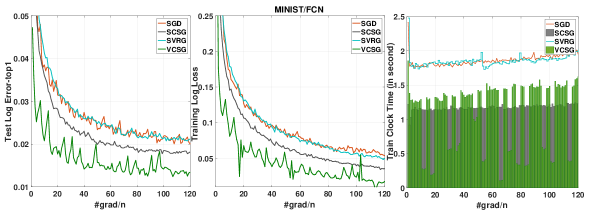
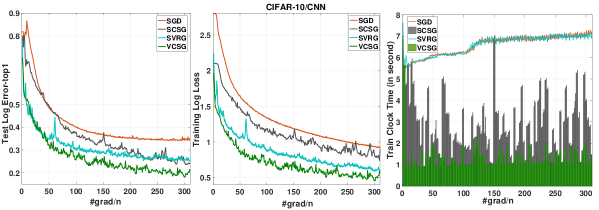
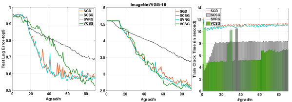
Fig.1 compares the performance of four methods, including SGD, SVRG, SCSG, and VCSG, via test log error, training log loss, and training time usage. It has two baselines in all sub-figures, including the performance of SVRG and SGD. The performance of SCSG test error and training loss is smaller than SGD on MNIST and CIFAR-10 data sets, consistent with the experimental results shown in [1]. However, in the ImageNet data set, which is a relatively larger scale application than the previous two data sets, the performance of SCSG becomes worse than SVRG and SGD, which showed weak robustness in our experiments. By contrast, VCSG shown as the green colour in all three datasets, has the lowest test error and training loss among all methods. In the ImageNet data set, both the test error of VCSG is initially higher than SVRG and SGD, but VCSG can reduce the test error and loss dramatically after around 75 epochs. One possible explanation is that the algorithm changes the batch size to the first term resulting in an escape from a local minima by increasing the variance to find a better solution. The right-hand column of Fig.1 presents the time usage, and it can be seen that SVRG and SGD are similar, having higher training time than the other two methods in all three data sets.
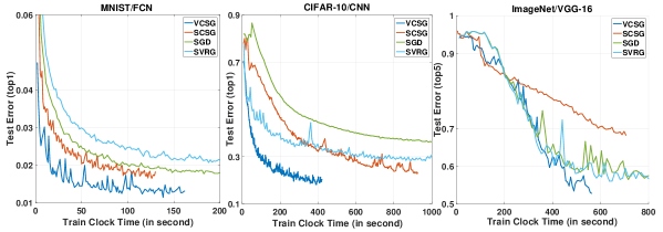
In Fig.2, we use a more visualized format to show the time usage in Fig.1. We can see in three sub-figures VCSG can achieve the lowest test error over a shorter time. To achieve the 0.025 top-1 test error in the MNIST data set, VCSG only takes 16 seconds around faster than SCSG, 3 faster than SVRG, and faster than SGD. In CIFAR-10 to achieve 0.3 top-1 test error, VCSG is around faster than SVRG, faster than SCSG and faster than SGD. In the ImageNet data set, to achieve 0.55 top-5 test error, VCSG can be faster than other methods by up to .
5 Discussion
In this paper, we proposed a VR-based optimization for non-convex problems. We theoretically determined that a hyper-parameter in each iteration can control the reduced variance of SVRG and balance the trade-off between a biased and an unbiased estimator. Meanwhile, an adjustable batch bounded by controlled reduced variance can work with , step size, and mini-batch to choose an appropriate estimator to converge faster to a stationary point on non-convex problems. Moreover, to verify our theoretical results, our experiments use three datasets on three DL models to present the performance of VCSG via test error/loss and elapsed time and compare these with other leading results. Both theoretical and experimental results show that VCSG can efficiently accelerate convergence. We believe that our algorithm is worthy of further study for non-convex optimization, particularly in deep neural networks training in large-scale applications.
Appendix A Technique lemmas
The first two lemmas we will use in our theorems are from Lemma A.1 and Lemma A.2 in [1].
Lemma A.1.
Let be an arbitrary population of N vectors with
Further let be a uniform random subset of with size m. Then
The geometric random variable has the key properties below.
Lemma A.2.
Let for some . Then for any sequence with ,
The below lemma will be useful to proof our lemmas.
Lemma A.3.
Let and , and a hyper-parameter . Then,
| (14) |
which should satisfied the below conditions:
Proof.
In the left side of Eq.14,
| (15) | ||||
Let the last line of Eq. 15 minus , we have
| (16) | ||||
Eq. 14 can be hold when the above equation less than . The first term in the last line of Eq. 16 is positive. For the second and third term, it has two cases. If the first case that the second term as , Eq. 14 can be hold when third term . Thus in the first case. Else if the second case that the term as , Eq. 14 can be hold when third term . Thus in the second case. ∎
Appendix B One-Epoch Analysis
B.1 Unbiased Estimator Version
Our algorithm is based on the SVRG method, thus the hyper-parameter should be within the range as in both unbiased and biased cases. We provide all useful lemmas we will applied in our proof of theorems at first, and provide a proof sketch for guidance. We start by bounding the gradient in Lemma B.1 and the variance in Lemma B.2.
Lemma B.1.
Under Definition 2.1,
Proof.
Using the fact that for a random variable Z , we have
| (17) | ||||
By Lemma A.1,
| (18) | ||||
where the last but one line is used Lemma A.3 when satisfied the condition that if , should be in the range . Otherwise, should be in the range . And the last line is based on Definition 2.1, then the bound of the gradient can be alternatively written as,
| (19) |
∎
Lemma B.2.
Proof.
Based on Lemma B.1 and the observation that is independent of , the bound of variance can be expressed as
| (20) | ||||
where the upper bound of the variance of the stochastic gradients . ∎
Lemma B.3.
Proof.
By Definition 2.1, we have
| (21) | ||||
Let denote the expectation ,…, given since is independent of them and let k= in Inq. 21. As ,… are independent of and taking the expectation with respect to and using Fubini’s theorem, Inq. 21 implies that
| (22) | ||||
where the last equation in Inq. 22 follows from Lemma A.2. The lemma substitutes by . ∎
Lemma B.4.
Suppose , then under Definition 2.1,
Proof of Theorem 3.1
Theorem.
Let and . Suppose for all , then under Definition 2.1, the output of Alg 2 we have
where and is positive when and .
Proof.
Multiplying Eq.B.3 by 2 and Eq.B.4 by and summing them, then we have,
| (31) | ||||
Using the fact that for any , in Inq. 31 can be bounded as
| (32) | ||||
Then Inq. 31 can be expressed as
| (33) | ||||
Since , and where and by Eq. 10, a one part in left hand side of above inequality can be simplified and positive as following:
| (34) | ||||
By Eq.34, the left side of Inq. 33 can be simplified since the factor of geometry distribution as
| (35) | ||||
Eq.35 is positive when and . Moreover, [34, 35] determined the learning rate that which can guarantees the convergence in non-convex case. In our case, satisfies within the range . Then Eq.33 can be simplified by Eq.35 as
| (36) | ||||
Then, using Lemma B.2, Inq. 36 can be rewritten as
| (37) |
B.2 Biased Estimator Version
We still provide all useful lemmas we will applied in our proof of theorems at first, and provide a proof sketch for guidance. For the biased estimation version, we still start by bounding the gradient in Lemma B.6 and the variance in Lemma B.7.
Lemma B.6.
Under Definition 2.1,
Lemma B.7.
where and .
Proof.
Based on Lemma A.1 and the observation that is independent of
| (41) | ||||
where the upper bound of the variance of the stochastic gradients .In above function, as is the expectation value of , we use to alternative for easily understanding later proof. Meanwhile, We can achieve the third equation in above function since the fact that . ∎
Lemma B.8.
Proof.
By Definition 2.1, we have
| (42) | ||||
Let denote the expectation ,…, given since is independent of them and let k= in Inq 42. As ,… are independent of and taking the expectation with respect to and using Fubini’s theorem, Inq. 42 implies that
| (43) | ||||
where the last equation in Inq. 43 follows from Lemma A.2. The lemma substitutes by . ∎
Lemma B.9.
Suppose , then under Definition lsmooth1,
Proof of Theorem 3.2
Theorem.
Proof.
Multiplying Eq.B.8 by 2 and Eq.B.9 by and summing them, then we have,
| (51) | ||||
Using the fact that for any , in Inq. 51 can be bounded as
| (52) | ||||
Then Inq. 51 can be rewritten as
| (53) | ||||
Since , and where , we have
| (54) | ||||
By Eq. 54, the left side of Inq. 53 can be simplified as
| (55) | ||||
Eq.55 is positive when and . Moreover, [34, 35] determined the learning rate that which can guarantees the convergence in non-convex case. In our case, should satisfy the range , thus .
Appendix C Convergence Analysis for L-smooth Objectives
Under the specifications of Theorem 3.1, Theorem 3.2 and Definition 2.1, the output can achieve its upper bound of gradients depending on two estimators.
Proof.
After achieved the result in above, and specified parameters, we can obtain result of Theorem 3.3.
References
- [1] Lihua Lei, Cheng Ju, Jianbo Chen, and Michael I Jordan. Non-convex finite-sum optimization via scsg methods. In I. Guyon, U. V. Luxburg, S. Bengio, H. Wallach, R. Fergus, S. Vishwanathan, and R. Garnett, editors, Advances in Neural Information Processing Systems 30, pages 2348–2358. Curran Associates, Inc., 2017.
- [2] R. G. Strongin and Y. D. Sergeyev. Global Optimization with Non-Convex Constraints - Sequential and Parallel Algorithms (Nonconvex Optimization and Its Applications Volume 45) (Nonconvex Optimization and Its Applications). Springer-Verlag, Berlin, Heidelberg, 2000.
- [3] Sashank J. Reddi, Ahmed Hefny, Suvrit Sra, Barnabás Póczós, and Alex Smola. Stochastic variance reduction for nonconvex optimization. In Proceedings of the 33rd International Conference on International Conference on Machine Learning - Volume 48, ICML’16, pages 314–323. JMLR.org, 2016.
- [4] Alekh Agarwal and Léon Bottou. A lower bound for the optimization of finite sums. In Proceedings of the 32nd International Conference on Machine Learning, ICML 2015, Lille, France, 6-11 July 2015, pages 78–86, France, 2015. JMLR Workshop and Conference Proceedings.
- [5] Chao Qu, Yan Li, and Huan Xu. Non-convex conditional gradient sliding. volume 80 of Proceedings of Machine Learning Research, pages 4208–4217, Stockholmsmässan, Stockholm Sweden, 10–15 Jul 2018. PMLR.
- [6] P. McCullagh and J. A. Nelder. Generalized Linear Models. Chapman & Hall / CRC, London, 1989.
- [7] Alexei A. Gaivoronski. Convergence properties of backpropagation for neural nets via theory of stochastic gradient methods. part 1. Optimization Methods and Software, 4(2):117–134, 1994.
- [8] D. Bertsekas. A new class of incremental gradient methods for least squares problems. SIAM Journal on Optimization, 7(4):913–926, 1997.
- [9] P. Tseng. An incremental gradient(-projection) method with momentum term and adaptive stepsize rule. SIAM Journal on Optimization, 8(2):506–531, 1998.
- [10] Saeed Ghadimi and Guanghui Lan. Accelerated gradient methods for nonconvex nonlinear and stochastic programming. Math. Program., 156(1-2):59–99, 2016.
- [11] Rie Johnson and Tong Zhang. Accelerating stochastic gradient descent using predictive variance reduction. In C. J. C. Burges, L. Bottou, M. Welling, Z. Ghahramani, and K. Q. Weinberger, editors, Advances in Neural Information Processing Systems 26, pages 315–323. Curran Associates, Inc., 2013.
- [12] Aaron Defazio, Francis R. Bach, and Simon Lacoste-Julien. SAGA: A fast incremental gradient method with support for non-strongly convex composite objectives. CoRR, abs/1407.0202, 2014.
- [13] S. J. Reddi, S. Sra, B. Póczos, and A. Smola. Fast incremental method for smooth nonconvex optimization. In 2016 IEEE 55th Conference on Decision and Control (CDC), pages 1971–1977, Dec 2016.
- [14] Dongruo Zhou, Pan Xu, and Quanquan Gu. Stochastic nested variance reduced gradient descent for nonconvex optimization. In S. Bengio, H. Wallach, H. Larochelle, K. Grauman, N. Cesa-Bianchi, and R. Garnett, editors, Advances in Neural Information Processing Systems 31, pages 3921–3932. Curran Associates, Inc., 2018.
- [15] Cong Fang, Chris Junchi Li, Zhouchen Lin, and Tong Zhang. Spider: Near-optimal non-convex optimization via stochastic path-integrated differential estimator. In S. Bengio, H. Wallach, H. Larochelle, K. Grauman, N. Cesa-Bianchi, and R. Garnett, editors, Advances in Neural Information Processing Systems 31, pages 689–699. Curran Associates, Inc., 2018.
- [16] Yossi Arjevani, Yair Carmon, John C. Duchi, Dylan J. Foster, Nathan Srebro, and Blake E. Woodworth. Lower bounds for non-convex stochastic optimization. CoRR, abs/1912.02365, 2019.
- [17] Jia Bi and Steve R. Gunn. A stochastic gradient method with biased estimation for faster nonconvex optimization. In Abhaya C. Nayak and Alok Sharma, editors, PRICAI 2019: Trends in Artificial Intelligence, pages 337–349, Cham, 2019. Springer International Publishing.
- [18] Percy Liang, Francis R. Bach, Guillaume Bouchard, and Michael I. Jordan. Asymptotically optimal regularization in smooth parametric models. In Advances in Neural Information Processing Systems 22: 23rd Annual Conference on Neural Information Processing Systems 2009. Proceedings of a meeting held 7-10 December 2009, Vancouver, British Columbia, Canada., pages 1132–1140, 2009.
- [19] Han-Fu Chen, Lei Guo, and Ai-Jun Gao. Convergence and robustness of the robbins-monro algorithm truncated at randomly varying bounds. Stochastic Processes and their Applications, 27:217 – 231, 1987.
- [20] Jie Chen and Ronny Luss. Stochastic gradient descent with biased but consistent gradient estimators. CoRR, abs/1807.11880, 2018.
- [21] Jie Chen, Tengfei Ma, and Cao Xiao. Fastgcn: Fast learning with graph convolutional networks via importance sampling. CoRR, abs/1801.10247, 2018.
- [22] Han fu Chen and AI-JUN Gao. Robustness analysis for stochastic approximation algorithms. Stochastics and Stochastic Reports, 26(1):3–20, 1989.
- [23] Naman Agarwal, Zeyuan Allen Zhu, Brian Bullins, Elad Hazan, and Tengyu Ma. Finding approximate local minima faster than gradient descent. 2016.
- [24] Zeyuan Allen-Zhu. Natasha 2: Faster non-convex optimization than sgd. In S. Bengio, H. Wallach, H. Larochelle, K. Grauman, N. Cesa-Bianchi, and R. Garnett, editors, Advances in Neural Information Processing Systems, volume 31, pages 2675–2686. Curran Associates, Inc., 2018.
- [25] Yurii Nesterov. Introductory Lectures on Convex Optimization: A Basic Course. Springer Publishing Company, Incorporated, 1 edition, 2014.
- [26] Zeyuan Allen-Zhu and Elad Hazan. Variance reduction for faster non-convex optimization. volume 48 of Proceedings of Machine Learning Research, pages 699–707, New York, New York, USA, 20–22 Jun 2016. PMLR.
- [27] Y Nesterov. Introductory lectures on convex optimization: A basic course. 01 2003.
- [28] Arkadi Nemirovski, Anatoli B. Juditsky, Guanghui Lan, and Alexander Shapiro. Robust stochastic approximation approach to stochastic programming. SIAM Journal on Optimization, 19(4):1574–1609, 2009.
- [29] Sharon L. Lohr. Sampling: Design and analysis. Technometrics, 42, 05 2000.
- [30] Reza Babanezhad, Mohamed Osama Ahmed, Alim Virani, Mark W. Schmidt, Jakub Konecný, and Scott Sallinen. Stop wasting my gradients: Practical SVRG. CoRR, abs/1511.01942, 2015.
- [31] Marek Niezgoda. Laguerre–samuelson type inequalities. Linear Algebra and its Applications, 422(2):574 – 581, 2007.
- [32] Karen Simonyan and Andrew Zisserman. Very deep convolutional networks for large-scale image recognition. CoRR, abs/1409.1556, 2014.
- [33] Olga Russakovsky, Jia Deng, Hao Su, Jonathan Krause, Sanjeev Satheesh, Sean Ma, Zhiheng Huang, Andrej Karpathy, Aditya Khosla, Michael Bernstein, Alexander C. Berg, and Li Fei-Fei. ImageNet Large Scale Visual Recognition Challenge. International Journal of Computer Vision (IJCV), 115(3):211–252, 2015.
- [34] Lihua Lei, Cheng Ju, Jianbo Chen, and Michael I. Jordan. Non-convex finite-sum optimization via SCSG methods. In NIPS, pages 2345–2355, 2017.
- [35] Lihua Lei and Michael Jordan. Less than a Single Pass: Stochastically Controlled Stochastic Gradient. In Aarti Singh and Jerry Zhu, editors, Proceedings of the 20th International Conference on Artificial Intelligence and Statistics, volume 54 of Proceedings of Machine Learning Research, pages 148–156, Fort Lauderdale, FL, USA, 20–22 Apr 2017. PMLR.