Anytime Diagnosis for Reconfiguration

Abstract

Many domains require scalable algorithms that help to determine diagnoses efficiently and often within predefined time limits. Anytime diagnosis is able to determine solutions in such a way and thus is especially useful in real-time scenarios such as production scheduling, robot control, and communication networks management where diagnosis and corresponding reconfiguration capabilities play a major role. Anytime diagnosis in many cases comes along with a trade-off between diagnosis quality and the efficiency of diagnostic reasoning. In this paper we introduce and analyze FlexDiag which is an anytime direct diagnosis approach. We evaluate the algorithm with regard to performance and diagnosis quality using a configuration benchmark from the domain of feature models and an industrial configuration knowledge base from the automotive domain. Results show that FlexDiag helps to significantly increase the performance of direct diagnosis search with corresponding quality tradeoffs in terms of minimality and accuracy.

Keywords: Anytime Diagnosis, Reconfiguration, Direct Diagnosis, Constraint Solving, Configuration, Software Product Lines.

1 Introduction

Knowledge-based configuration is one of the most successful application areas of Artificial Intelligence felfernighotzbagleytiihonen2014 ; frayman1987 ; saphaag ; hvam2008 ; Sabin1998 ; SalvadorForza2007 ; Stumptner . There exist many application domains ranging from telecommunication systems ffhs98b ; cocos1994 , railway interlocking systems SiemensStudy , the automotive domain SinzKaiserKuechlin:03 ; varisales ; WalterKuechlin2014 , software product lines benavides10 to the configuration of services ServiceConfiguration .

Configuration technologies must be able to deal with inconsistencies which can occur in different contexts. First, a configuration knowledge base can be inconsistent, i.e., no solution can be determined. In this context, the task of knowledge engineers is to figure out which constraints are responsible for the unintended behavior of the knowledge base. Bakker et al. paperBakker1993 show how to apply model-based diagnosis Reiter1987 to determine minimal sets of constraints in a knowledge base that are responsible for a given inconsistency. A variant thereof is documented in Felfernig et al. felfernig2004 where an approach to the automated debugging of knowledge bases with test cases is introduced. Test cases are interpreted as positive or negative examples that describe the intended behavior of a knowledge base. If some positive examples induce conflicts in the configuration knowledge base, some of the constraints in the knowledge base are faulty and have to be adapted or deleted. If some negative examples are accepted (i.e., not rejected) by the configuration knowledge base, further constraints have to be included in order to take these examples into account (in Felfernig et al. felfernig2004 this issue is solved by simply including negative examples in negated form into the configuration knowledge base). A related approach in the area of software product lines is proposed in benavides10-diagnosis . Second, customer requirements can be inconsistent with the underlying knowledge base. Felfernig et al. felfernig2004 also show how to diagnose customer requirements that are inconsistent with a configuration knowledge base. The underlying assumption is that the configuration knowledge base itself is consistent but combined with a set of requirements is inconsistent.

The so far mentioned configuration-related diagnosis approaches are based on conflict-directed hitting set determination where conflicts have to be calculated in order to be able to derive one or more corresponding diagnoses cr91 ; Janota2014 ; junker04quickxplain ; Reiter1987 ; Shah2011 . These approaches often determine diagnoses in a breadth-first search manner which allows the identification of minimal cardinality diagnoses. The major disadvantage of applying these approaches is the need of determining minimal conflicts which is inefficient especially in cases where only the leading diagnoses (the most relevant ones) are sought. Furthermore, in many application domains it is not necessarily the case that minimal cardinality diagnoses are the preferred ones – Felfernig et al. felfernig2009 show how recommendation technologies JannachZankerFelfernigFriedrich2010 can be exploited for guiding the search for preferred (minimal but not necessarily minimal cardinality) diagnoses.

Algorithms based on the idea of anytime diagnosis are useful in scenarios where diagnoses have to be provided in real-time, i.e., within given time limits. Efficient diagnosis and reconfiguration of communication networks is crucial to retain the quality of service, i.e., if some components/nodes in a network fail, corresponding substitutes and extensions have to be determined immediately SimulationReconfiguration ; Stumptner99reconfiguration . In today’s production scenarios which are characterized by small batch sizes and high product variability, it is increasingly important to develop algorithms that support the efficient reconfiguration of schedules. Such functionalities support the paradigm of smart production, i.e., the flexible and efficient production of highly variant products. Further applications are the diagnosis and repair of robot control software SteinbauerRobocup2005 , sensor networks pc99 , feature models Janota2014 ; benavides10-diagnosis , the reconfiguration of cars WalterKuechlin2013 , and the reconfiguration of buildings Friedrich2011 . In the diagnosis approach presented in this paper, we assure diagnosis determination within certain time limits by systematically reducing the number of solver calls needed. This specific interpretation of anytime diagnosis requires a trade-off between diagnosis quality (evaluated, e.g., in terms of minimality) and the time needed for diagnosis determination.

Algorithmic approaches to provide efficient solutions for diagnosis problems are manyfold. Some approaches focus on improvements of Reiter’s original hitting set directed acyclic graph (HSDAG) Reiter1987 in terms of a personalized computation of leading diagnoses deKleerAIJournal1990 or other extensions that make the basic approach Reiter1987 more efficient Wotawa2001 . Wang et al. Wang2009 introduce an approach to derive binary decision diagrams (BDDs) Andersen2010 ; Bryant1992 on the basis of a pre-determined set of conflicts – diagnoses can then be determined by finding paths in the BDD that include given variable settings (e.g., requirements defined by the user). A predefined set of conflicts can also be compiled into a corresponding linear optimization problem Fijany2004 ; diagnoses can then be determined by solving the given problem. In knowledge-based recommendation scenarios, diagnoses for user requirements can be pre-compiled in such a way that for a given set of customer requirements, the diagnosis search task can be reduced to querying a relational table (see, for example, JannachContent2006 ; Schubert2011 ). All of the mentioned approaches either extend the approach of Reiter Reiter1987 or improve efficiency by exploiting pre-generated information about conflicts or diagnoses.

An alternative to conflict-directed diagnosis Reiter1987 are direct diagnosis algorithms that determine minimal diagnoses without the need of predetermining minimal conflict sets felfernig2012 ; kostya2014 . The FastDiag algorithm felfernig2012 is a divide-and-conquer based algorithm that supports the determination of diagnoses without a preceding conflict detection. Such direct diagnosis approaches are especially useful in situations where not the complete set of diagnoses has to be determined but users are interested in the leading diagnoses, i.e., diagnoses with a high probability of being relevant for the user. Also in the context of SAT solving, algorithms have been developed that allow the efficient determination of diagnoses (also denoted as minimal correction subsets) in an efficient fashion Bacchus2014 ; Gregoire2014 ; Silva2013 ; Mencia2015 . Beside efficiency, prediction quality of a diagnosis algorithm is a major issue in interactive configuration settings, i.e., those diagnoses have to be identified that are relevant for the user. A corresponding comparison of approaches to determine preferred minimal diagnoses and unsatisfied clauses with minimum total weights is provided in Walter2016 . The authors point out theoretical commonalities and prove the reducibility of both concepts to each other.

In this paper we show how the FastDiag approach can be converted into an anytime diagnosis algorithm (FlexDiag) that allows tradeoffs between diagnosis quality (minimality and accuracy) and performance. In this paper we focus on reconfiguration scenarios Friedrich2011 ; SimulationReconfiguration ; Stumptner99reconfiguration ; WalterKuechlin2014 , i.e., we show how FlexDiag can be applied in situations where a given configuration (solution) has to be adapted conform to a changed set of customer requirements. Our contributions in this paper are the following. First, based on previous work on the diagnosis of inconsistent knowledge bases, we show how to solve reconfiguration tasks with direct diagnosis. Second, we make direct diagnosis anytime-aware by including a parametrization that helps to systematically limit the number of consistency checks and thus make diagnosis search more efficient. Finally, we report the results of a FlexDiag-related evaluation conducted on the basis of real-world configuration knowledge bases (feature models and configuration knowledge bases from the automotive industry) and discuss quality properties of related diagnoses not only in terms of minimality but also in terms of accuracy.

The remainder of this paper is organized as follows. In Section 2 we introduce an example configuration knowledge base from the domain of resource allocation. This knowledge base will serve as a working example throughout the paper. Thereafter (Section 3) we introduce a definition of a reconfiguration task. In Section 4 we discuss basic principles of direct diagnosis on the basis of FlexDiag and show how this algorithm can be applied in reconfiguration scenarios. In Section 5 we present the results of an analysis of algorithm performance and the quality of determined diagnoses. A simple example of the application of FlexDiag in production environments is given in Section 6. In Section 7 we discuss issues for future work. With Section 8 we conclude the paper.

2 Example Configuration Knowledge Base

A configuration system determines configurations (solutions) on the basis of a given set of customer requirements KnowledgeRepresentation . In many cases, constraint satisfaction problem (CSP) representations are used for the definition of a configuration task. A configuration task and a corresponding configuration (solution) can be defined as follows:

Definition 1 (Configuration Task and Configuration). A configuration task can be defined as a CSP ($V,D,C\cup R$) where $V=\{v_{1},v_{2},...,v_{n}\}$ is a set of variables, $D=\bigcup_{v_{i}\in V}\{dom(v_{i})\}$ represents domain definitions, and $C=\{c_{1},c_{2},...,c_{m}\}$ is a set of constraints (the configuration knowledge base). Additionally, user requirements are represented by a set of constraints $R=\{r_{1},r_{2},...,r_{k}\}$ where $R$ and $C$ are disjoint. A configuration (solution) for a configuration task is a complete set of assignments (constraints) $S=\{s_{1}:v_{1}=a_{1},s_{2}:v_{2}=a_{2},...,s_{n}:v_{n}=a_{n}\}$ where $a_{i}\in dom(v_{i})$ which is consistent with $C\cup R$.

An example of a configuration task represented as a constraint satisfaction problem (CSP) is the following.

Example (Configuration Task). In this resource allocation problem example, items (a barrel of fuel, a stack of paper, a pallet of fireworks, a pallet of personal computers, a pallet of computer games, a barrel of oil, a pallet of roof tiles, and a pallet of rain pipes) have to be assigned to three different containers. There are a couple of constraints ($c_{i}$) to be taken into account, for example, fireworks must not be combined with fuel ($c_{1}$). Furthermore, there is one requirement ($r_{1}$) which indicates that the pallet of fireworks has to be assigned to container 1. On the basis of this configuration task definition, a configurator can determine a configuration (solution) $S$.

• $V=\{fuel,paper,fireworks,pc,games,oil,roof,pipes\}$

• $dom(fuel)=dom(paper)=dom(fireworks)=dom(pc)=dom(games)=dom(oil)=dom(roof)=dom(pipes)=\{1,2,3\}$

• $C=\{c_{1}:fireworks\neq fuel,c_{2}:fireworks\neq paper,\\ ~{}~{}~{}~{}~{}~{}~{}~{}~{}~{}~{}~{}c_{3}:fireworks\neq oil,c_{4}:pipes=roof,c_{5}:paper\neq fuel\}$

• $R=\{r_{1}:fireworks=1\}$

• $S=\{s_{1}:pc=3,s_{2}:games=1,s_{3}:paper=2,s_{4}:fuel=3,\\ ~{}~{}~{}~{}~{}~{}~{}~{}~{}~{}~{}~{}s_{5}:fireworks=1,s_{6}:oil=2,s_{7}:roof=1,s_{8}:pipes=1\}$

On the basis of the given definition of a configuration task, we now introduce the concept of reconfiguration (see also Friedrich2011 ; SimulationReconfiguration ; Stumptner99reconfiguration ; WalterKuechlin2014 ).

3 Reconfiguration Task

It can be the case that an existing configuration $S$ has to be adapted due to new customer requirements. Examples thereof are changing requirements in production schedules, failing components or overloaded network infrastructures in a mobile phone network, and changes in the internal model of the environment of a robot. In the following we assume that the pallet of paper should be reassigned to container 3 and the personal computer and games pallets should be assigned to the same container. Formally, the set of new requirements is represented by $R_{\rho}:\{r_{1}^{\prime}:pc=games,r_{2}^{\prime}:paper=3\}$. In order to determine reconfigurations, we have to calculate a corresponding diagnosis $\Delta$ (see Definition 2).

Definition 2 (Diagnosis). A diagnosis $\Delta$ (correction subset) is a subset of $S=\{s_{1}:v_{1}=a_{1},s_{2}:v_{2}=a_{2},...,s_{n}:v_{n}=a_{n}\}$ such that $S-\Delta\cup C\cup R_{\rho}$ is consistent. $\Delta$ is minimal if there does not exist a diagnosis $\Delta^{\prime}$ with $\Delta^{\prime}\subset\Delta$.

On the basis of the definition of a minimal diagnosis, we can introduce a formal definition of a reconfiguration task.

Definition 3 (Reconfiguration Task and Reconfiguration). A reconfiguration task can be defined as a CSP ($V,D,C,S,R_{\rho}$) where $V$ is a set of variables, $D$ represents variable domain definitions, $C$ is a set of constraints, $S$ represents an existing configuration, and $R_{\rho}=\{r_{1}^{\prime},r_{2}^{\prime},...,r_{q}^{\prime}\}$ ($R_{\rho}$ consistent with $C$) represents a set of reconfiguration requirements. Furthermore, let $\Delta$ be a minimal diagnosis for the reconfiguration task. A reconfiguration is a variable assignment $S_{\Delta}$ = $\{s_{1}:v_{1}=a_{1}^{\prime},s_{2}:v_{2}=a_{2}^{\prime},...,s_{l}:v_{l}=a_{l}^{\prime}\}$ where $s_{i}\in\Delta$, $a_{i}^{\prime}\neq a_{i}$, and $S-\Delta\cup S_{\Delta}\cup C\cup R_{\rho}$ is consistent.

If $R_{\rho}$ is inconsistent with $C$, the new requirements have to be analyzed and changed before a corresponding reconfiguration task can be triggered felfernigAIMAG2011 ; felfernig2009 . An example of a reconfiguration task in the context of our configuration knowledge base is the following.

Example (Reconfiguration Task). In the resource allocation problem, the original customer requirements $R$ are substituted by the requirements $R_{\rho}=\{r_{1}^{\prime}:pc=games,r_{2}^{\prime}:paper=3\}$. The resulting reconfiguration task instance is the following.

• $V=\{fuel,paper,fireworks,pc,games,oil,roof,pipes\}$

• $dom(fuel)=dom(paper)=dom(fireworks)=dom(pc)=dom(games)=dom(oil)=dom(roof)=dom(pipes)=\{1,2,3\}$

• $C=\{c_{1}:fireworks\neq fuel,c_{2}:fireworks\neq paper,\\ ~{}~{}~{}~{}~{}~{}~{}~{}~{}~{}~{}~{}c_{3}:fireworks\neq oil,c_{4}:pipes=roof,c_{5}:paper\neq fuel\}$

• $S=\{s_{1}:pc=3,s_{2}:games=1,s_{3}:paper=2,s_{4}:fuel=3,\\ ~{}~{}~{}~{}~{}~{}~{}~{}~{}~{}~{}~{}s_{5}:fireworks=1,s_{6}:oil=2,s_{7}:roof=1,s_{8}:pipes=1\}$

• $R_{\rho}=\{r_{1}^{\prime}:pc=games,r_{2}^{\prime}:paper=3\}$

To solve a reconfiguration task (see Definition 3), conflict-directed diagnosis approaches Reiter1987 would determine a set of minimal conflicts and then determine a hitting set that resolves each of the identified conflicts. In this context, a minimal conflict set $CS\subseteq S$ is a minimal set of variable assignments that trigger an inconsistency with $C\cup R_{\rho}$, i.e., $CS\cup C\cup R_{\rho}$ is inconsistent and there does not exist a conflict set $CS^{\prime}$ with $CS^{\prime}\subset CS$. In our working example, the minimal conflict sets are $CS_{1}:\{s_{1}:pc=3,s_{2}:games=1\}$, $CS_{2}:\{s_{3}:paper=2\}$, and $CS_{3}:\{s_{4}:fuel=3\}$. The corresponding minimal diagnoses are $\Delta_{1}:\{s_{1},s_{3},s_{4}\}$ and $\Delta_{2}:\{s_{2},s_{3},s_{4}\}$.

The elements in a diagnosis indicate which variable assignments have to be adapted such that a reconfiguration can be determined that takes into account the new requirements in $R_{\rho}$. Consequently, a reconfiguration represents a minimal set of changes to the original configuration ($S$) such that the new requirements $R_{\rho}$ are taken into account. If we choose $\Delta_{1}$, a reconfiguration $S_{\Delta}$ (reassignments for the variable assignments in $\Delta_{1}$) can be determined by a CSP solver call $C\cup R_{\rho}\cup(S-\Delta_{1})$. The resulting configuration $S^{\prime}$ can be $\{s_{1}:pc=1,s_{2}:games=1,s_{3}:paper=3,s_{4}:fuel=2,s_{5}:fireworks=1,s_{6}:oil=2,s_{7}:roof=1,s_{8}:pipes=1\}$. For a detailed discussion of conflict-based diagnosis we refer to Reiter Reiter1987 . In the following we introduce an approach to the determination of minimal reconfigurations which is based on a direct diagnosis algorithm, i.e., diagnoses are determined without the need of determining related minimal conflict sets.

4 Reconfiguration with FlexDiag

In the following discussions, the set $AC=C\cup R_{\rho}\cup S$ represents the union of all constraints that restrict the set of possible solutions for a given reconfiguration task. Furthermore, $S$ represents a set of constraints that are considered as candidates for being included in a diagnosis $\Delta$. The idea of FlexDiag (Algorithm 1) is to systematically filter out the constraints that become part of a minimal diagnosis using a divide-and-conquer based approach.

Algorithm 1

1:procedure FlexDiag($S,AC=C\cup R_{\rho}\cup S,m$): $\Delta$

2:     if isEmpty($S$) or inconsistent($AC-S$) then

3:         return $\emptyset$;

4:     else

5:         return FlexD($\emptyset$,$S$,$AC$,$m$);

6:     end if

7:end procedure

8:

9:procedure FlexD($D,S=\{s_{1}..s_{q}\},AC,m$): $\Delta$

10:     if $D\neq\emptyset$ and consistent ($AC$) then

11:         return $\emptyset$;

12:     else if size($S$) $\leq$ $m$ then

13:         return $S$;

14:     end if

15:     $k=\lceil\frac{q}{2}\rceil$;

16:     $S_{1}=\{s_{1}..s_{k}\};S_{2}=\{s_{k+1}..s_{q}\}$;

17:     $D_{1}=\textsc{FlexD}(S_{1},S_{2},AC-S_{1},m)$;

18:     $D_{2}=\textsc{FlexD}(D_{1},S_{1},AC-D_{1},m)$;

19:     $return(D_{1}\cup D_{2})$;

20:end procedure

Sketch of Algorithm. In our example reconfiguration task, the original configuration $S=\{s_{1},s_{2},s_{3},$ $s_{4},s_{5},s_{6},s_{7},s_{8}\}$ and the new set of customer requirements is $R_{\rho}=\{r_{1}^{\prime},r_{2}^{\prime}\}$. Since $S\cup R_{\rho}\cup C$ is inconsistent, we are in need of a minimal diagnosis $\Delta$ and a reconfiguration $S_{\Delta}$ such that $S-\Delta\cup S_{\Delta}\cup R_{\rho}\cup C$ is consistent. In the following we will show how the FlexDiag (Algorithm 1) can be applied to determine such a minimal diagnosis $\Delta$.

FlexDiag is assumed to be activated under the assumption that $AC=C\cup R_{\rho}\cup S$ is inconsistent, i.e., the consistency of $AC$ is not checked by the algorithm. If $AC$ is inconsistent but $AC-S$ is also inconsistent, FlexDiag will not be able to identify a diagnosis in $S$; therefore $\emptyset$ is returned. Otherwise, a recursive function FlexD is activated which is in charge of determining one minimal diagnosis $\Delta\subseteq S$. In each recursive step, the constraints in $S$ are divided into two different subsets ($S_{1}$ and $S_{2}$) in order to figure out if already one of these subsets includes a diagnosis. If this is the case, the second set must not be inspected for diagnosis elements anymore. If we assume, for example, $S=\{s_{1},s_{2},s_{3},s_{4},s_{5},s_{6},s_{7},s_{8}\}$ is inconsistent and we divide $S$ into the two subsets $S_{1}=\{s_{1},s_{2},s_{3},s_{4}\}$ and $S_{2}=\{s_{5},s_{6},s_{7},s_{8}\}$ and $S_{1}$ is already consistent with $C\cup R_{\rho}$ then diagnosis elements are searched in $S_{2}$ (since $S_{1}$ is already consistent). The complete related walkthrough is depicted in Figures 1 and 2.

FlexDiag is based on the concepts of FastDiag felfernig2012 , i.e., it returns one diagnosis ($\Delta$) at a time and is complete in the sense that if a diagnosis is contained in $S$, then the algorithm will find it. A corresponding reconfiguration can be determined by a CSP solver call $C\cup R_{\rho}\cup(S-\Delta)$. The determination of multiple diagnoses at a time can be realized on the basis of the construction of a HSDAG Reiter1987 . In FlexDiag, the parameter $m$ is used to control diagnosis quality in terms of minimality, accuracy, and the performance of diagnostic search (see Section 5). The higher the value of $m$ the higher the performance of FlexDiag and the lower the degree of diagnosis quality. The inclusion of $m$ to control quality and performance is the major difference between FlexDiag and FastDiag. If $m=1$ (see Algorithm 1), the number of consistency checks needed for determining one minimal diagnosis is $2\delta\times log_{2}(\frac{n}{\delta})+2\delta$ (in the worst case) felfernig2012 . In this context, $\delta$ represents the set size of the minimal diagnosis $\Delta$ and $n$ represents the number of constraints in solution $S$.

If $m>1$, the number of needed consistency checks can be systematically reduced if we accept the tradeoff of possibly loosing the property of diagnosis minimality (see Definition 2). If we allow settings with $m>1$, we can reduce the upper bound of the number of consistency checks to $2\delta\times log_{2}(\frac{2n}{\delta\times m})$ (in the worst case). These upper bounds regarding the number of needed consistency checks allow to estimate the worst case runtime performance of the diagnosis algorithm which is extremely important for real-time scenarios. Consequently, if we are able to estimate the upper limit of the time needed for completing one consistency check (e.g., on the basis of simulations with an underlying constraint solver), we are also able to figure out lower bounds for $m$ that must be chosen in order to guarantee a FlexDiag runtime within predefined time limits.

Table 1 depicts an overview of consistency checks needed depending on the setting of the parameter $m$ and the diagnosis size $\delta$ for $|S|=16$. For example, if $m=2$ and the size of a minimal diagnosis is $\delta=4$, then the upper bound for the number of needed consistency checks is 16. If the size of $\delta$ further increases, the number of corresponding consistency checks does not increase anymore. Figures 1 and 2 depict FlexDiag search trees depending on the setting of granularity parameter $m$. The upper bound for the number of consistency checks helps us to determine the maximum amount of time that will be needed to determine a diagnosis on the basis of FlexDiag. For example, if the maximum time needed for one consistency check is $20ms$, the maximum time needed for determining a diagnosis with $m=2$ (given $\delta=8$) is $\approx 320$ milliseconds.

$\delta$	m=1	m=2	m=4	m=8
1	10	8	6	4
2	16	12	8	4
4	24	16	8	-
8	32	16	-	-
16	32	-	-	-

Table 1: Worst-case estimates for the number of needed consistency checks depending on the granularity parameter $m$ and the diagnosis size $\delta$ for $|S|=16$.

FlexDiag determines one diagnosis at a time which indicates variable assignments of the original configuration that have to be changed such that a reconfiguration conform to the new requirements ($R_{\rho}$) is possible. The algorithm supports the determination of leading diagnoses, i.e., diagnoses that are preferred with regard to given user preferences felfernig2012 ; Walter2016 . FlexDiag is based on a strict lexicographical ordering of the constraints in $S$: the lower the importance of a constraint $s_{i}\in S$ the lower the index of the constraint in $S$. For example, $s_{1}:pc=3$ has the lowest ranking. The lower the ranking, the higher the probability that the constraint will be part of a reconfiguration $S_{\Delta}$. Since $s_{1}$ has the lowest priority and it is part of a conflict, it is element of the diagnosis returned by FlexDiag. For a discussion of the properties of lexicographical orderings we refer to felfernig2012 ; junker04quickxplain .

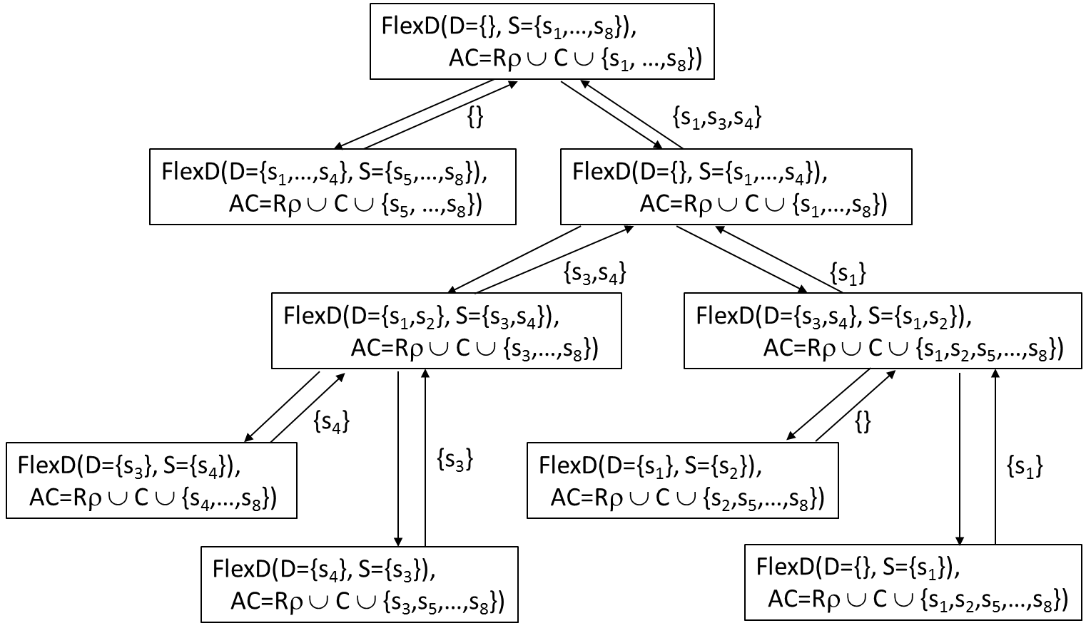
Figure 1: FlexDiag walkthrough: determining one minimal diagnosis with $m=1$ ($\Delta=\{s_{1},s_{3},s_{4}\}$).

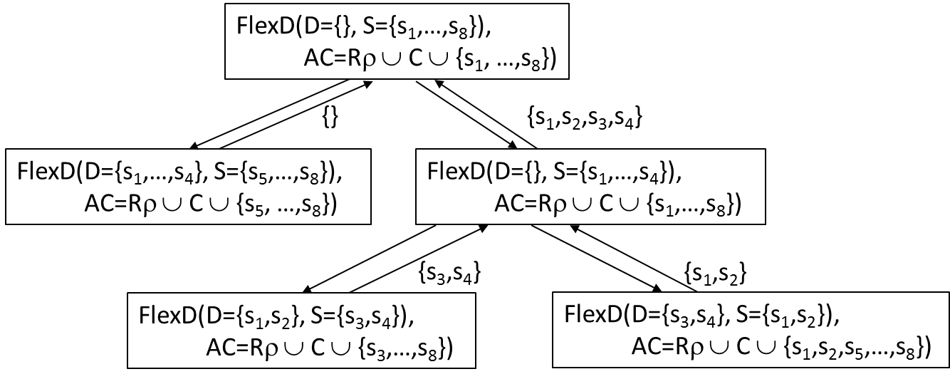
Figure 2: FlexDiag walkthrough: determining a minimal diagnosis with $m=2$ ($\Delta=\{s_{1},s_{2},s_{3},s_{4}\}$).

5 Evaluation

In this section, we present the evaluation we executed to verify the performance of FlexDiag. We first analyze how FlexDiag performs in front of real and randomly generated models and then, compare it with an evolutionary approach.

5.1 Evaluation aspects

To evaluate FlexDiag, we analyzed the two aspects of (1) algorithm performance (in terms of milliseconds needed to determine one minimal diagnosis) and (2) diagnosis quality (in terms of minimality and accuracy – see Formulae 1 and 2). We analyzed both aspects by varying the value of parameter $m$. Our hypothesis in this context was that the higher the value of $m$, the lower the number of needed consistency checks (the higher the efficiency of diagnosis search) and the lower diagnosis quality in terms of the share of diagnosis-relevant constraints returned by FlexDiag. Diagnosis quality can, for example, be measured in terms of the degree of minimality of the constraints in a diagnosis $\Delta$ (see Formula 1), i.e., the cardinality of $\Delta$ compared to the cardinality of $\Delta_{min}$. $|\Delta_{min}|$ represents the cardinality of a minimal diagnosis identified with $m=1$.

$$minimality(\Delta)=\frac{|\Delta_{min}|}{|\Delta|}$$ (1)

If $m>1$, there is no guarantee that the diagnosis $\Delta$ determined for $S$ is a superset of the diagnosis $\Delta_{min}$ determined for $S$ in the case $m=1$. Besides minimality, we introduce accuracy as an additional quality indicator (see Formula 2). The higher the share of elements of $\Delta_{min}$ in $\Delta$, the higher the corresponding accuracy (the algorithm is able to reproduce the elements of the minimal diagnosis for $m=1$).

$$accuracy(\Delta)=\frac{|\Delta\cap\Delta_{min}|}{|\Delta_{min}|}$$ (2)

5.2 Datasets and Results

We evaluated FlexDiag with regard to both metrics (algorithm performance, and diagnosis quality) by applying the algorithm to different benchmarks. First, using random feature models generated with the Betty tool betty . Second, with the set of models hosted in the S.P.L.O.T repository. Third, in a real-world model extracted from the last Ubuntu Linux distribution galindo10-acota . Finally, a real-world automotive dataset. The configuration models are feature models which include requirement constraints, compatibility constraints, and different types of structural constraints such as mandatory relationships and alternatives.

For all the different datasets we report on averaged values. For that, we first, calculate the acurracy, execution time, and minimality for all the executions. Then, we aggregate the data and calculate the mean for the metrics.

5.2.1 Experimental platform

The experiments were conducted using a version of FlexDiag implemented in Java and integrated in the FaMa Tool Suite benavides2013fama . All the models were translated to a Constraint Satisfaction Problem (CSP) and used the Choco library for consistency checking. Further, our FlexDiag implementation was running in a grid of computers running on four-CPU Dell Blades with Intel Xeon X5560 CPUs running at 2.8GHz, with 8 threads per CPU, and CentOS v6. The total RAM memory was 8GB. To parallelize the executions we used GNU Parallel Tange2011a .

5.2.2 Random models

The first dataset used to evaluate FlexDiag was randomly generated. We used BeTTy betty to generate a dataset that ranges from 50 to 2000 features and 10% to 30% of cross-tree constraints. The generation approach is based on Thüm et al. thum2009reasoning that imitates realistic topologies.

For each model combining a given number of features and a percentage of cross-tree constraints, we randomly generated different sizes of reconfiguration requirements that involved the 10%, 30%, 50% and 100% of features of the model. Then we randomly reordered each of the reconfiguration requirements 10 times (to prevent ordering biases). Moreover, we executed FlexDiag on each combination of parameters three times to get average execution times trying to avoid third party threads.

In the following, we present the results showing a comparison between the different values of m and how the values evolved depending on the size of the models. Note that to generate the plots we aggregated the data and therefore the values shown are averaged results.

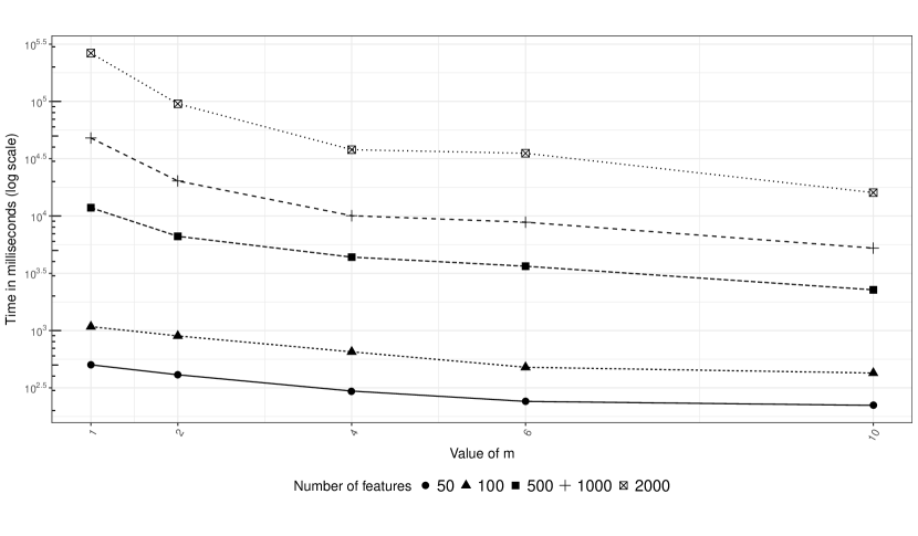
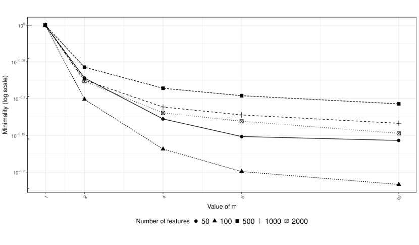
Figure 3: Random evolution based on features, time and m

Figure 3 shows how the diagnosis performance can be increased depending on the setting of the m parameter. Also we observe how the minimality deteriorates when increasing m.

Table 2: Random evaluation depending on m value and model size. $|V|$ represents the number of variables in the CSP. The second column shows the $m$ value used in FlexDiag. $|C|$ refers to the number of constraints in the model, $|\Delta|$ is the average size of a diagnosis, and average time (in milliseconds), average minimality, and average accuracy represent the means of the calculated values for those metrics.

$|V|$	m	$|C|$	$|\Delta|$	Average time	Average minimality	Average accuracy
50	1	58.40	14.62	501.63	1.00	1.00
	2		15.72	410.92	0.85	0.92
	4		17.22	296.14	0.75	0.87
	6		18.71	240.52	0.71	0.87
	10		19.07	222.15	0.70	0.86
100	1	109.80	27.51	1081.24	1.00	0.99
	2		32.80	896.99	0.79	0.90
	4		38.19	651.20	0.68	0.88
	6		40.99	477.64	0.63	0.87
	10		42.29	425.16	0.61	0.88
500	1	566.40	182.62	11808.41	1.00	1.00
	2		203.77	6647.27	0.88	0.96
	4		219.41	4372.98	0.82	0.95
	6		221.82	3643.81	0.80	0.96
	10		231.49	2265.53	0.78	0.97
1000	1	1141.00	347.25	47956.27	1.00	1.00
	2		398.62	20227.16	0.84	0.97
	4		434.76	10051.52	0.77	0.96
	6		440.64	8825.81	0.75	0.96
	10		461.53	5242.34	0.74	0.98
2000	1	2274.80	663.36	264084.35	1.00	1.00
	2		743.21	95467.42	0.84	0.97
	4		818.12	37911.86	0.76	0.97
	6		828.39	35271.86	0.74	0.96
	10		888.38	16000.95	0.71	0.97

Table 2 shows the averaged data we obtained. It is worth mentioning that the minimality decreases when m increases and that accuracy still provides acceptable results with m = 10. Also, the execution time (in milliseconds) is less than five minutes in the worst case.

As we can observe in Table 2 and Figure 3, while the execution time decreases when incrementing $m$, quality deteriorates. However, minimality is clearly affected while accuracy stays with minor variations. Also, we observe that the time improvement depends on $m$ and the number of features. For example, if we compare the time between $m=1$ and $m=10$, we can increase in runtime of 2.26$\times$ for 50 features, 5.21$\times$ for 500 features, 9.14$\times$ for 1000 and 16.5$\times$ for 2000 features.

5.2.3 SPLOT repository models

We extracted a total of 387 models from the SPLOT repository. For each model, we randomly generated different sizes of reconfiguration requirements that involved the 10%, 30%, 50% and 100% of features of the model. Then we randomly reordered each of the reconfiguration requirements 10 times (to prevent ordering biases). Moreover, we executed FlexDiag on each combination of parameters three times to get average execution times trying to avoid third party threads.

Table 3 shows the data of those models categorized as realistic in the repository. We again see that FlexDiag scales with no problem offering a good trade-off between accuracy and minimality while keeping the average runtime (in milliseconds) below a second.

Table 3: FlexDiag results in front of SPLOT realistic models. $|V|$ represents the number of variables in the CSP. The second column shows the $m$ value used in FlexDiag. Model Name is the model name in SPLOT. $|C|$ refers to the number of constraints in the model, $|\Delta|$ is the average size of a diagnosis, and average time (in milliseconds), average minimality, and average accuracy represent the means of the calculated values for those metrics.

$|V|$	m	Model Name	$|C|$	$|\Delta|$	Average time	Average minimality	Average accuracy
290	1	REAL-FM-4	61.00	1.00	527.45	1.00	1.00
	2			1.75	527.83	0.62	1.00
	4			2.75	464.33	0.48	1.00
	6			4.00	444.65	0.40	1.00
	10			6.25	432.65	0.35	1.00
88	1	REAL-FM-1	26.00	6.93	566.92	1.00	1.00
	2			10.48	514.35	0.62	0.86
	4			15.02	411.55	0.42	0.76
	6			21.17	316.52	0.32	0.70
	10			22.58	317.92	0.28	0.70
44	1	REAL-FM-20	8.00	3.50	225.32	1.00	0.99
	2			5.35	201.23	0.60	0.86
	4			8.07	171.22	0.38	0.84
	6			10.15	155.45	0.31	0.80
	10			10.90	152.78	0.28	0.80
23	1	REAL-FM-2	9.00	2.78	177.55	1.00	1.00
	2			4.07	161.72	0.68	0.86
	4			4.93	144.05	0.54	0.82
	6			6.60	131.78	0.41	0.76
	10			7.62	216.98	0.36	0.76
43	1	REAL-FM-3	13.00	1.75	211.97	1.00	1.00
	2			3.03	199.62	0.60	0.95
	4			4.78	178.35	0.36	0.93
	6			7.38	161.82	0.24	0.92
	10			9.15	147.82	0.21	0.88

As we can observe in Table 3, while the execution time decreases when incrementing m, quality deteriorates again. However minimality is clearly affected while accuracy stays with minor variations, although, we can observe some special cases (”REAL-FM-5” with $m=2$) were it deteriorates a bit more.

5.2.4 Ubuntu-based model

In order to test FlexDiag with large-scale real models, we encoded the variability existing in the Debian packaging system for the Ubuntu distribution and generated a set of configurations representing Ubuntu user installations with wrong package selections. Concretely, we modelled the Ubuntu Xenial distribution containing 58,107 packages and 52,721 constraints. This model was extracted using the mapping presented in galindo10-acota ; galindo10-fmsple . We executed FlexDiag with different m values. We randomly generated different sizes of reconfiguration requirements that involved the 10%, 30%, 50% and 100% of features of the model. Then we randomly reordered each of the reconfiguration requirements 10 times (to prevent ordering biases). Moreover, we executed FlexDiag on each combination of parameters three times to get average execution times trying to avoid third party threads.

Table 4 shows that FlexDiag is able to provide a good accuracy even with m set to 10. Also, it shows as expected, the negative impact of m regarding minimality. We observe that the execution time with $m=1$ was $3.7$ hours while with $m=10$ it was $2.5$ hours. This represents an improvement of runtime in 1.47$\times$.

Table 4: Results obtained after executing FlexDiag with the Ubuntu Xenial variability model. The seconds column shows the $m$ value used in FlexDiag. $|V|$ represents the number of variables in the CSP. $|C|$ refers to the number of constraints in the CSP, $|\Delta|$ is the average size of a diagnosis, and average time (in milliseconds), average minimality, and average accuracy represent the means of the calculated values for those metrics.

$|V|$	m	$|C|$	$|\Delta|$	Average time	Average minimality	Average accuracy
58107	1	105459	1.75	13523986.27	1.00	1.00
	2		3.40	12245231.77	0.51	0.75
	4		6.12	10800288.33	0.31	0.71
	6		7.15	10546545.60	0.24	0.71
	10		12.48	9208147.25	0.14	0.71

5.2.5 Automotive models

The benchmark used in this experiment includes three automotive configuration models from a German car manufacturer. For each model, we randomly generated different sizes of reconfiguration requirements that involved the 10%, 30%, 50% and 100% of features of the model. Then we randomly reordered each of the reconfiguration requirements 10 times (to prevent ordering biases). Moreover, we executed FlexDiag on each combination of parameters three times to get average execution times trying to avoid third party threads.

Table 5: FlexDiag evaluated with benchmarks from the automotive industry (calculation of the first diagnosis: $ids$ 1–3 represent different type series of a German premium car manufacturer). The second column shows the $m$ value used in FlexDiag. $|V|$ represents the number of variables in the CSP. $|C|$ refers to the number of constraints in the CSP, $|\Delta|$ is the average size of a diagnosis, and average time (in milliseconds), average minimality, and average accuracy represent the means of the calculated values for those metrics.

id	m	$|V|$	$|C|$	$|\Delta|$	Average time	Average minimality	Average accuracy
01	1	1888	7404	623.78	22812981.47	1.00	1.00
	2			787.43	6720901.40	0.80	0.99
	4			870.25	1785352.90	0.71	0.99
	6			876.97	1716644.85	0.70	0.99
	10			892.85	473017.90	0.69	1.00
02	1	1828	5451	611.38	8730834.77	1.00	1.00
	2			760.85	3176414.95	0.81	0.99
	4			845.47	914621.30	0.72	0.99
	6			850.28	878283.40	0.71	1.00
	10			865.22	237203.47	0.70	1.00
03	1	1843	8056	369.00	22147386.47	1.00	1.00
	2			538.50	11901657.38	0.80	0.98
	4			605.00	3381818.66	0.70	0.99
	6			613.31	3104191.16	0.68	0.99
	10			626.59	823533.78	0.67	0.99

Table 5 shows that FlexDiag is able to provide a good accuracy even with m set to 10. Again, it shows as expected, the negative impact of m regarding minimality. Also, the execution time for model with $id=1$ and $m=1$ was $6.33$ hours while with $m=10$ it was $7.9$ minutes. This represents an improvement of 26.9$\times$.

5.3 Comparing FlexDiag with Evolutionary Algorithms

In this research we do not compare FlexDiag with more traditional diagnosis approaches – for related evaluations we refer the reader to felfernig2012 were detailed analyses can be found. These analyses clearly indicate that direct diagnosis approaches outperform standard diagnosis approaches based on the resolution of minimal conflicts Reiter1987 (if the search goal is to identify not all minimal but the so-called leading diagnoses which should, for example, be shown to users in interactive settings).

However, in this Section we compare FlexDiag with an evolutionary algorithm inspired by cendic2014genetic ; li2002computing . The evolutionary algorithm has been build with the jenetics framework for Java leaving all parameters default and fixing the process to 500 generations. Also we compare the performance of FlexDiag with m set to 1 to have a fair comparison. Note that with higher values of m, we would even perform better in terms of runtime.

The first observation is that the evolutionary approach was not capable of dealing with very large realistic models (Ubuntu, automotive) when setting a time-out of 24 hours. Therefore, we report this comparison only relying on randomly generated models.

Figure 4 shows that the required time for FlexDiag is usually higher for models having less than 500 features. Therefore, there is a point when FlexDiag pays off and scales much better. Also, it is worth mentioning that the evolutionary algorithm was not capable of obtaining a complete and minimal explanation and returned only partial diagnoses. This is, in 500 generations it only found partial explanations.

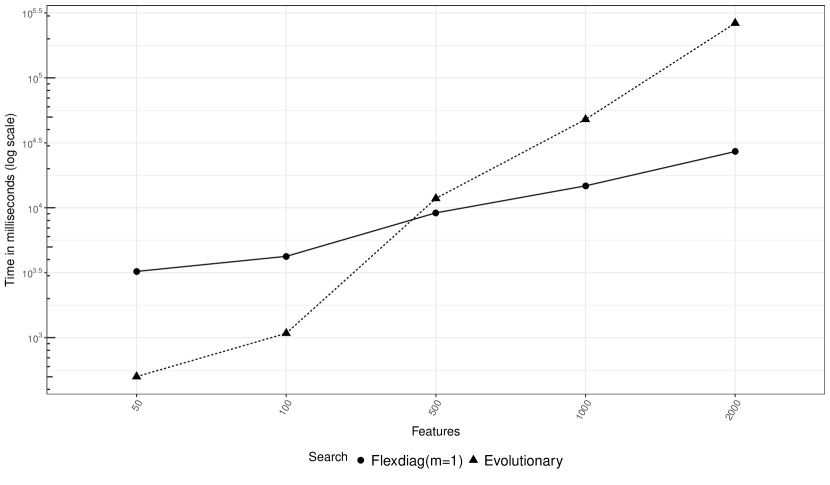
Figure 4: Comparison between FlexDiag and the evolutionary approach regarding time

Table 6 shows that FlexDiag returns minimal diagnoses while we observe that the evolutionary approach was not capable of detecting minimal diagnoses. Also, we do see that FlexDiag offered a much better accuracy.

Table 6: Comparison results of the evolutionary approach and FlexDiag. $|V|$ represents the number of variables in the CSP. Approach refers to the used approach, $|C|$ refers to the number of constraints in the CSP, $|\Delta|$ is the average size of a diagnosis, and average time (in milliseconds), average minimality, and average accuracy represent the means of the calculated values for those metrics.

$|V|$	Approach	$|C|$	$|\Delta|$	Average time	Average minimality	Average accuracy
50	Evolutionary	58.40	1.53	3237.87	8.84	0.33
50	FlexDiag	58.40	14.62	501.63	1.00	1.00
100	Evolutionary	109.80	2.13	4229.25	10.81	0.17
100	FlexDiag	109.80	27.51	1081.24	1.00	0.99
500	Evolutionary	566.40	9.45	9142.43	15.82	0.03
500	FlexDiag	566.40	182.62	11808.41	1.00	1.00
1000	Evolutionary	1141.00	22.07	14754.50	11.49	0.03
1000	FlexDiag	1141.00	347.25	47956.27	1.00	1.00
2000	Evolutionary	2274.80	48.61	27111.93	9.32	0.03
2000	FlexDiag	2274.80	663.36	264084.35	1.00	1.00

5.4 Threats to validity

Even though the experiments presented in this paper provide evidence that the solution proposed is valid, there are some assumptions that we made that may affect their validity. In this section, we discuss the different threats to validity that affect the evaluation.

External validity. The inputs used for the experiments presented in this paper were either realistic or designed to mimic realistic feature models. The Debian feature model and the Automotive are realistic since numerous experts were involved in the design. However, since they were developed using a manual design process, it may have errors and not encode all configurations. Also, the random feature models may not accurately reflect the structure of real feature models used in industry. The major threats to the external validity are:

• Population validity, the real feature models that we used may not represent all valid configurations in the domains due it manual construction. Also, random models might not have the same structure as real models (e.g. mathematical operators used in the complex constraints). To reduce these threats to validity, we generated the models using previously published techniques thum2009reasoning and using existing implementations of these techniques in Betty betty .

• Ecological validity: While external validity, in general, is focused on the generalization of the results to other contexts (e.g. using other models), the ecological validity ii focused on possible errors in the experiment materials and tools used. To prevent ecological validity threats, such as third party threads running in the virtual machines and impacting performance, the FlexDiag analyses were executed three times and then averaged.

Internal validity The CPU resources required to analyse a feature model depend on the number of features and percentage of cross-tree constraints. However, there may be other variables that affect performance, such as the nature of the constraints used. To minimize these other possible effects, we introduced a variety of models to ensure that we covered a large part of the constraint space.

5.5 Final Remarks

We observed that FlexDiag scales up with random and real-world feature models. Observing that, generally, diagnosis quality in terms of minimality and accuracy deteriorates with an increasing size of parameter $m$.

Minimality and accuracy depend on the configuration domain and are not necessarily monotonous. For example, since a diagnosis determined by FlexDiag is not necessarily a superset of a diagnosis determined with $m=1$, it can be the case that the minimality of a diagnosis determined with $m>1$ is greater than 1 (if FlexDiag determines a diagnosis with lower cardinality than the minimal diagnosis determined with $m=1$). For simplicity, let us assume that $AC=S=\{c_{1},c_{2},c_{3},c_{4},c_{5},c_{6},c_{7},c_{8}\}$ and the following conflict sets $CS_{i}$ exist between the constraints $c_{i}\in S$: $CS_{1}:\{c_{1},c_{3}\}$, $CS_{2}:\{c_{2},c_{3}\}$, and $CS_{3}:\{c_{4},c_{6}\}$. Given $m=1$, FlexDiag would determine the diagnosis $\{c_{1},c_{2},c_{4}\}$ whereas in the case of $m=2$, $\{c_{3},c_{4}\}$ is returned by the algorithm.

6 Another Example: Reconfiguration in Production

The following simplified reconfiguration task is related to scheduling in production where it is often the case that, for example, schedules and corresponding production equipment has to be reconfigured. In this example setting, we do not take into account configurable production equipment (configurable machines) and limit the reconfiguration to the assignment of orders to corresponding machines. The assignment of an order $o_{i}$ to a certain machine $m_{j}$ is represented by the corresponding variable $o_{i}m_{j}$. The domain of each such variable represents the different possible slots in which an order can be processed, for example, $o_{1}m_{1}=1$ denotes the fact that the processing of order $o_{1}$ on machine $m_{1}$ is performed during and finished after time slot 1.

Further constraints restrict the way in which orders are allowed to be assigned to machines, for example, $o_{1}m_{1}<o_{1}m_{2}$ denotes the fact that order $o_{1}$ must be completed on machine $m_{1}$ before a further processing is started on machine $m_{2}$. Furthermore, no two orders must be assigned to the same machine during the same time slot, for example, $o_{1}m_{1}\neq o_{2}m_{1}$ denotes the fact that order $o_{1}$ and $o_{2}$ must not be processed on the same machine in the same time slot (slots 1..3). Finally, the definition of our reconfiguration task is completed with an already determined schedule $S$ and a corresponding reconfiguration request represented by the reconfiguration requirement $R_{\rho}=\{r_{1}^{\prime}:o_{3}m_{3}<5\}$, i.e., order $o_{3}$ should be completed within less than 5 time units.

• $V=\{o_{1}m_{1},o_{1}m_{2},o_{1}m_{3},o_{2}m_{1},o_{2}m_{2},o_{2}m_{3},o_{3}m_{1},o_{3}m_{2},o_{3}m_{3}\}$

• $dom(o_{1}m_{1})=dom(o_{2}m_{1})=dom(o_{3}m_{1})=\{1,2,3\}.$ $dom(o_{1}m_{2})=dom(o_{2}m_{2})=dom(o_{3}m_{2})=\{2,3,4\}.$ $dom(o_{1}m_{3})=dom(o_{2}m_{3})=dom(o_{3}m_{3})=\{3,4,5\}.$

• $C=\{c_{1}:o_{1}m_{1}<o_{1}m_{2},c_{2}:o_{1}m_{2}<o_{1}m_{3},\\ ~{}~{}~{}~{}~{}~{}~{}~{}~{}~{}~{}$ $c_{3}:o_{2}m_{1}<o_{2}m_{2},c_{4}:o_{2}m_{2}<o_{2}m_{3},$ $c_{5}:o_{3}m_{1}<o_{3}m_{2},\\ ~{}~{}~{}~{}~{}~{}~{}~{}~{}~{}~{}$ $c_{6}:o_{3}m_{2}<o_{3}m_{3},$ $c_{7}:o_{1}m_{1}\neq o_{2}m_{1},\\ ~{}~{}~{}~{}~{}~{}~{}~{}~{}~{}~{}~{}c_{8}:o_{1}m_{1}\neq o_{3}m_{1},c_{9}:o_{2}m_{1}\neq o_{3}m_{1},\\ ~{}~{}~{}~{}~{}~{}~{}~{}~{}~{}~{}~{}c_{10}:o_{1}m_{2}\neq o_{2}m_{2},c_{11}:o_{1}m_{2}\neq o_{3}m_{2},\\ ~{}~{}~{}~{}~{}~{}~{}~{}~{}~{}~{}~{}c_{12}:o_{2}m_{2}\neq o_{3}m_{2},c_{13}:o_{1}m_{3}\neq o_{2}m_{3},\\ ~{}~{}~{}~{}~{}~{}~{}~{}~{}~{}~{}~{}c_{14}:o_{1}m_{3}\neq o_{3}m_{3},c_{15}:o_{2}m_{3}\neq o_{3}m_{3}\}$

• $S=\{s_{1}:o_{1}m_{1}=1,s_{2}:o_{1}m_{2}=2,s_{3}:o_{1}m_{3}=3,\\ ~{}~{}~{}~{}~{}~{}~{}~{}~{}~{}~{}s_{4}:o_{2}m_{1}=2,s_{5}:o_{2}m_{2}=3,s_{6}:o_{2}m_{3}=4,\\ ~{}~{}~{}~{}~{}~{}~{}~{}~{}~{}~{}s_{7}:o_{3}m_{1}=3,s_{8}:o_{3}m_{2}=4,s_{9}:o_{3}m_{3}=5\}$

• $R_{\rho}=\{r_{1}^{\prime}:o_{3}m_{3}<5\}$

This reconfiguration task can be solved using FlexDiag. If we keep the ordering of the constraints as defined in $S$, FlexDiag (with $m=1$) returns the diagnosis $\Delta:\{s_{1},s_{2},s_{3},s_{7},s_{8},s_{9}\}$ which can be used to determine the new solution $S^{\prime}=\{s_{1}:o_{1}m_{1}=3,s_{2}:o_{1}m_{2}=4,s_{3}:o_{1}m_{3}=5,s_{4}:o_{2}m_{1}=2,s_{5}:o_{2}m_{2}=3,s_{6}:o_{2}m_{3}=4,s_{7}:o_{3}m_{1}=1,s_{8}:o_{3}m_{2}=2,s_{9}:o_{3}m_{3}=3\}$ (see Table 7). If we change the parametrization to $m=2$, FlexDiag returns the same diagnosis but in approximately half of the time (with 10 iterations, $16$ milliseconds were needed on an average for $m=2$ whereas $31$ milliseconds were needed for $m=1$). This is consistent with the estimates in Table 1.

Possible ordering criteria for constraints in such rescheduling scenarios can be, for example, customer value (changes related to orders of important customers should occur with a significantly lower probability) and the importance of individual orders. If some orders in a schedule should not be changed, this can be achieved by simply defining such requests as requirements ($R_{\rho}$), i.e., change requests as well as stability requests can be included as constraints $r_{i}^{\prime}$ in $R_{\rho}$.

$S$	$S^{\prime}$
$s_{1}:o_{1}m_{1}=1$	$s_{1}:o_{1}m_{1}=3$
$s_{4}:o_{2}m_{1}=2$	$s_{4}:o_{2}m_{1}=2$
$s_{7}:o_{3}m_{1}=3$	$s_{7}:o_{3}m_{1}=1$
$s_{2}:o_{1}m_{2}=2$	$s_{2}:o_{1}m_{2}=4$
$s_{5}:o_{2}m_{2}=3$	$s_{5}:o_{2}m_{2}=3$
$s_{8}:o_{3}m_{2}=4$	$s_{8}:o_{3}m_{2}=2$
$s_{3}:o_{1}m_{3}=3$	$s_{3}:o_{1}m_{3}=5$
$s_{6}:o_{2}m_{3}=4$	$s_{6}:o_{2}m_{3}=4$
$s_{9}:o_{3}m_{3}=5$	$s_{9}:o_{3}m_{3}=3$

Table 7: Reconfiguration determined for rescheduling task – $S$ represents the original configuration and $S^{\prime}$ represents a configuration resulting from a reconfiguration task.

7 Future Work

In our work, we focused on the evaluation of reconfiguration scenarios where the knowledge base itself is assumed to be consistent. In future work, we will extend the FlexDiag algorithm to make it applicable in scenarios where knowledge bases are tested felfernig2004 . An example issue is to take into account situations where unintended configurations are accepted by the knowledge base. In this context, we will extend the work of felfernig2004 by not only taking into account negative test cases but also automatically generate relevant test cases, for example, on the basis of mutation testing approaches. We plan to extend our empirical evaluation to further industrial configuration knowledge bases. Furthermore, we want to analyze in which way we are able to further improve the output quality (e.g., in terms of minimality and accuracy) of FlexDiag, for example, by applying different constraint orderings depending on the observed interaction patterns (of users) and probability estimates for diagnosis membership derived thereof. The better potentially relevant constraints are predicted the better the diagnosis quality in terms of the mentioned metrics of minimality and accuracy. Note that, for example, counting the number of elements already identified as partial diagnosis elements in FlexDiag does not help to keep diagnosis determination within certain time limits, however, this mechanism could be used when determing more than one diagnosis to include diagnosis size as a relevance criterion. Also, in this context will analyze further alternatives to evaluate the quality of diagnoses which go beyond the metrics used in this article.

8 Conclusions

Efficient reconfiguration functionalities are needed in various scenarios such as the reconfiguration of production schedules, the reconfiguration of the settings in mobile phone networks, and the reconfiguration of robot context information. We analyzed the FlexDiag algorithm with regard to potentials of improving existing direct diagnosis algorithms. When using FlexDiag, there is a clear trade-off between performance of diagnosis calculation and diagnosis quality (measured, for example, in terms of minimality and accuracy).

References

- (1) H. Andersen, T. Hadzic, and D. Pisinger, ‘Interactive Cost Configuration Over Decision Diagrams’, Journal of Artificial Intelligence Research, 37, 99–139, (2010).
- (2) F. Bacchus, J. Davies, M. Tsimpoukell, and G. Katsirelos, ‘Relaxation Search: A Simple Way of Managing Optional Clauses’, in AAAI’2014, pp. 835–841, Quebec, Canada, (2014).
- (3) R. Bakker, F. Dikker, F. Tempelman, and P. Wogmim, ‘Diagnosing and Solving Over-determined Constraint Satisfaction Problems’, in 13th International Joint Conference on Artificial Intelligence, pp. 276–281, Chambery, France, (1993).
- (4) D. Benavides, S. Segura, and A. Ruiz-Cortes, ‘Automated Analysis of Feature Models 20 years Later: a Literature Review’, Information Systems, 35(6), 615–636, (2010).
- (5) D. Benavides, P. Trinidad, A. Ruiz-Cortés, and S. Segura, ‘Fama’, in Systems and Software Variability Management, 163–171, Springer, (2013).
- (6) R. Bryant, ‘Symbolic Boolean Manipulation with Ordered Binary-Decision Diagrams’, ACM Computing Surveys, 24(3), 293–318, (1992).
- (7) Bojana Ćendić-Lazović, ‘A Genetic Algorithm for the Minimum Hitting Set’, Scientific Publications of the State University of Novi Pazar Series A: Applied Mathematics, Informatics and mechanics, 6(2), 107–117, (2014).
- (8) J. Crow and J. Rushby, ‘Model-Based Reconfiguration: Toward an Integration with Diagnosis’, in 9th National Conference on Artificial Intelligence (AAAI-91), pp. 836–841, Anaheim, California, (1991). The MIT Press.
- (9) J. DeKleer, ‘Using Crude Probability Estimates to Guide Diagnosis’, AI Journal, 45(3), 381–391, (1990).
- (10) A. Falkner, A. Felfernig, and A. Haag, ‘Recommendation Technologies for Configurable Products’, AI Magazine, 32(3), 99–108, (2011).
- (11) A. Falkner and H. Schreiner, ‘SIEMENS: Configuration and Reconfiguration in Industry’, in Knowledge-based Configuration – From Research to Business Cases, eds., A. Felfernig, L. Hotz, C. Bagley, and J. Tiihonen, chapter 16, 251–264, Morgan Kaufmann Publishers, (2014).
- (12) A. Felfernig, G. Friedrich, D. Jannach, and M. Stumptner, ‘Consistency-based Diagnosis of Configuration Knowledge Bases’, Artificial Intelligence, 152(2), 213–234, (2004).
- (13) A. Felfernig, L. Hotz, C. Bagley, and J. Tiihonen, Knowledge-based Configuration: From Research to Business Cases, Elsevier/Morgan Kaufmann, 1st edn., 2014.
- (14) A. Felfernig, M. Schubert, G. Friedrich, M. Mandl, M. Mairitsch, and E. Teppan, ‘Plausible Repairs for Inconsistent Requirements’, in 21st International Joint Conference on Artificial Intelligence (IJCAI’09), pp. 791–796, Pasadena, CA, USA, (2009).
- (15) A. Felfernig, M. Schubert, and C. Zehentner, ‘An Efficient Diagnosis Algorithm for Inconsistent Constraint Sets’, Artificial Intelligence for Engineering Design, Analysis and Manufacturing (AI EDAM), 26(1), 53–62, (2012).
- (16) A. Fijany and F. Vatan, ‘New Approaches for Efficient Solution of Hitting Set Problem’, in International Symposium on Information and Communication Technologies, pp. 1–6, Cancun, Mexico, (2004).
- (17) G. Fleischanderl, G. Friedrich, A. Haselböck, H. Schreiner, and M. Stumptner, ‘Configuring Large Systems Using Generative Constraint Satisfaction’, IEEE Intelligent Systems, 13(4), 59–68, (1998).
- (18) F. Frayman and S. Mittal, ‘COSSACK: A Constraint-Based Expert System for Configuration Tasks’, in Knowledge Based Expert Systems in Engineering: Planning and Design, eds., D. Sriram and R. Adey, 143–166, Computational Mechanics Publications, Woburn, MA, USA, (1987).
- (19) G. Friedrich, A. Ryabokon, A. Falkner, A. Haselböck, G. Schenner, and H. Schreiner, ‘ (Re)configuration using Answer Set Programming’, in IJCAI 2011 Workshop on Configuration, pp. 17–24, (2011).
- (20) J. Galindo, D. Benavides, and S. Segura, ‘Debian Packages Repositories as Software Product Line Models. Towards Automated Analysis’, in ACoTA, pp. 29–34, (2010).
- (21) J. Galindo, F. Roos-Frantz, J. García-Galán, and A. Ruiz-Cortés, ‘Extracting Orthogonal Variability Models from Debian Repositories’, in Proc. of 2nd International Workshop on Formal Methods and Analysis in Software Product Line Engineering (FMSPLE 2011), co-located with Software Product Line Conference 2011 (SPLC 2011), pp. 8–8, Munich, (08/2011 2011). Fraunhofer, Fraunhofer.
- (22) E. Gregoire, J. Lagniez, and B. Mazure, ‘An Experimentally Efficient Method for (MSS, CoMSS) Partitioning’, in 28th AAAI Conference on Artificial Intelligence, pp. 2666–2673, Quebec, Canada, (2014).
- (23) A. Haag, ‘Product Configuration in SAP - A Personal Retrospective’, in Knowledge-based Configuration – From Research to Business Cases, eds., A. Felfernig, L. Hotz, C. Bagley, and J. Tiihonen, chapter 27, 389–411, Morgan Kaufmann Publishers, (2014).
- (24) L. Hotz, A. Felfernig, M. Stumptner, A. Ryabokon, C. Bagley, and K. Wolter, ‘Configuration Knowledge Representation & Reasoning’, in Knowledge-based Configuration – From Research to Business Cases, eds., A. Felfernig, L. Hotz, C. Bagley, and J. Tiihonen, chapter 6, 59–96, Morgan Kaufmann Publishers, (2014).
- (25) D. Jannach, ‘Finding Preferred Query Relaxations in Content-based Recommenders’, in 3rd Intl. IEEE Conference on Intelligent Systems, pp. 355–360, London, UK, (2006).
- (26) D. Jannach, M. Zanker, A. Felfernig, and G. Friedrich, Recommender Systems – An Introduction, Cambridge University Press, 2010.
- (27) M. Janota, G. Botterweck, and J. Marques-Silva, ‘On Lazy and Eager Interactive Reconfiguration’, in 8th International Workshop on Variability Modeling of Software-Intensive Systems, pp. 1–8, San Antonio, TX, USA, (2014).
- (28) U. Junker, ‘QuickXPlain: Preferred Explanations and Relaxations for Over-constrained problems’, in 19th Intl. Conference on Artifical Intelligence (AAAI’04), pp. 167–172. AAAI Press, (2004).
- (29) L. Hvam and N. Mortensen and H. Riis, Product Customization, Springer, 2008.
- (30) L. Li and J. Yunfei, ‘Computing Minimal Hitting Sets with Genetic Algorithm’, Technical report, Zhongshan (Sun Yatsen) University, China, (2002).
- (31) A. Mackworth, ‘Consistency in Networks of Relations’, Artificial Intelligence, 8(1), 99–118, (1977).
- (32) J. Marques-Silva, F. Heras, M. Janota, A. Previti, and A. Belov, ‘On Computing Minimal Correction Subsets’, in IJCAI 2013, pp. 615–622, Peking, China, (2013).
- (33) C. Mencia, A. Previti, and J. Marques-Silva, ‘Efficient Relaxations of Over-constrained CSPs’, in ICTAI’2014, pp. 725–732, (2014).
- (34) I. Nica, F. Wotawa, R. Ochenbauer, C. Schober, H. Hofbauer, and S. Boltek, ‘Kapsch: Reconfiguration of Mobile Phone Networks’, in Knowledge-based Configuration – From Research to Business Cases, eds., A. Felfernig, L. Hotz, C. Bagley, and J. Tiihonen, chapter 19, 287–300, Morgan Kaufmann, (2014).
- (35) G. Provan and Y. Chen, ‘Model-based Diagnosis and Control Reconfiguration for Discrete Event Systems: an Integrated Approach’, in Proceedings of the 38th IEEE Conference on Decision and Control, volume 2, pp. 1762–1768, Phoenix, AZ, USA, (1999).
- (36) R. Reiter, ‘A Theory of Diagnosis From First Principles’, Artificial Intelligence, 32(1), 57–95, (1987).
- (37) D. Sabin and R. Weigel, ‘Product Configuration Frameworks - A Survey’, IEEE Intelligent Systems, 13(4), 42–49, (1998).
- (38) F. Salvador and C. Forza, ‘Principles for Efficient and Effective Sales Configuration Design’, International Journal of Mass Customization, 2(1–2), 114–127, (2007).
- (39) M. Schubert and A. Felfernig, ‘BFX: Diagnosing Conflicting Requirements in Constraint-based Recommendation’, International Journal on Artificial Intelligence Tools, 20(2), 297–312, (2011).
- (40) S. Segura, J. Galindo, D. Benavides, J. Parejo, and A. Ruiz-Cortés, ‘BeTTy: Benchmarking and Testing on the Automated Analysis of Feature Models’, in Proceedings of the Sixth International Workshop on Variability Modeling of Software-Intensive Systems, VaMoS’12, pp. 63–71, New York, NY, USA, (2012). ACM.
- (41) I. Shah, ‘Direct Algorithms for Finding Minimal Unsatisfiable Subsets In Over-Constrained CSPs’, International Journal on Artificial Intelligence Tools, 20(1), 53–91, (2011).
- (42) K. Shchekotykhin, G. Friedrich, P. Rodler, and P. Fleiss, ‘Sequential Diagnosis of High-cardinality Faults in Knowledge Bases by Direct Diagnosis Generation’, in ECAI 2014, pp. 813–818, Prague, Czech Republic, (2014).
- (43) C. Sinz, A. Kaiser, and W. Küchlin, ‘Formal Methods for the Validation of Automotive Product Configuration Data’, Artificial Intelligence for Engineering Design, Analysis and Manufacturing, 17(1), 75–97, (2003).
- (44) G. Steinbauer, M. Mörth, and F. Wotawa, ‘Real-Time Diagnosis and Repair of Faults of Robot Control Software’, in RoboCup 2005, LNAI, pp. 13–23. Springer, (2005).
- (45) M. Stumptner, ‘An Overview of Knowledge-based Configuration’, AI Communications, 10(2), 111–126, (1997).
- (46) M. Stumptner, A. Haselböck, and G. Friedrich, ‘COCOS - A Tool for Constraint-based, Dynamic Configuration’, in 10th IEEE Conference on Artificial Intelligence for Applications (CAIA-94), pp. 373–380, San Antonio, TX, USA, (1994).
- (47) M. Stumptner and F. Wotawa, ‘Reconfiguration Using Model-based Diagnosis’, in 10th International Workshop on Principles of Diagnosis (DX-99), pp. 266–271, (1999).
- (48) O. Tange, ‘GNU Parallel – The Command-Line Power Tool’, ;login: The USENIX Magazine, 36(1), 42–47, (February 2011).
- (49) T. Thum, D. Batory, and C. Kastne, ‘Reasoning about edits to feature models’, in Software Engineering, 2009. ICSE 2009. IEEE 31st International Conference on, pp. 254–264. IEEE, (2009).
- (50) J. Tiihonen and A. Anderson, ‘VariSales’, in Knowledge-based Configuration – From Research to Business Cases, eds., A. Felfernig, L. Hotz, C. Bagley, and J. Tiihonen, chapter 26, 377–388, Morgan Kaufmann Publishers, (2014).
- (51) J. Tiihonen, W. Mayer, M. Stumptner, and M. Heiskala, ‘Configuring Services and Processes’, in Knowledge-based Configuration – From Research to Business Cases, eds., A. Felfernig, L. Hotz, C. Bagley, and J. Tiihonen, chapter 21, 313–324, Morgan Kaufmann Publishers, (2013).
- (52) R. Walter, A. Felfernig, and W. Küchlin, ‘Constraint-Based and SAT-Based Diagnosis of Automotive Configuration Problems’, Journal of Intelligent Information Systems (JIIS), 1–32, (2016).
- (53) R. Walter and W. Küchlin, ‘ReMax - A MaxSAT aided Product (Re-) Configurator’, in Workshop on Configuration 2014, pp. 55–66, (2014).
- (54) R. Walter, C. Zengler, and W. Küchlin, ‘Applications of MaxSAT in Automotive Configuration’, in Workshop on Configuration 2013, pp. 21–28, (2013).
- (55) K. Wang, Z. Li, Y. Ai, and Y. Zhang, ‘Computing Minimal Diagnosis with Binary Decision Diagrams Algorithm’, in 6th International Conference on Fuzzy Systems and Knowledge Discovery (FSKD’2009), pp. 145–149, (2009).
- (56) J. White, D. Benavides, D. Schmidt, P. Trinidad, B. Dougherty, and A. Ruiz-Cortez, ‘Automated Diagnosis of Feature Model Configurations’, Systems and Software, 83(7), 1094–1107, (2010).
- (57) F. Wotawa, ‘A Variant of Reiter’s Hitting-Set Algorithm’, Inf. Processing Letters, 79(1), 45–51, (2001).