Finite-size effects in response functions of molecular systems

Abstract.

We consider an electron in a localized potential submitted to a weak external, time-dependent field. In the linear response regime, the response function can be computed using Kubo’s formula. In this paper, we consider the numerical approximation of the response function by means of a truncation to a finite region of space. This is necessarily a singular approximation because of the discreteness of the spectrum of the truncated Hamiltonian, and in practice a regularization (smoothing) has to be used. Our results provide error estimates for the response function past the ionization threshold with respect to both the smoothing parameter and the size of the computational domain.

1. Introduction

Consider a molecule in its electronic ground state, to which an external time-dependent electric field is applied. The resulting change in the electronic density can be computed using linear response theory, resulting in a quantity $\widehat{K}(\omega)$ describing the response at frequency $\omega$. To compute it in practice, the domain of computation has to be truncated to a region of size $L$, yielding an approximate response function $\widehat{K}_{L}(\omega)$. Since the dynamics on the full space and on a finite region of space are qualitatively different, $\widehat{K}_{L}$ is qualitatively different from $\widehat{K}$: in particular, even when $\widehat{K}$ is a regular function, $\widehat{K}_{L}$ is always a singular distribution, reflecting the discreteness of the spectrum of the Hamiltonian. This paper answers, in a simplistic one-electron model, the following question: in which sense does $\widehat{K}_{L}$ converge to $\widehat{K}$, and with what convergence rate?

We focus here for technical convenience on the simplest continuous model of a single-electron system in a potential $V$, described by the rest Hamiltonian

(1) $$H=-\Delta+V,$$

with $V$ decaying at infinity in a sense to be made precise. The Hamiltonian $H$ is self-adjoint on $L^{2}(\mathbb{R}^{d})$, with possible negative eigenvalues and continuous spectrum $[0,\infty)$. Assume that there is a simple lowest eigenvalue $E_{0}<0$, with associated eigenfunction $\psi_{0}$. We consider the time-dependent Schrödinger equation

(2) $$i\partial_{t}\psi=H\psi+\varepsilon f(t)V_{\mathcal{P}}\psi,\quad\psi(0)=\psi_{0}$$

where $V_{\mathcal{P}}$ is a perturbing potential, $f$ a continuous causal function (i.e. $f(t)=0$ for $t<0$), and $\varepsilon>0$ is a small parameter. If $V_{\mathcal{O}}$ is a potential representing an observable, to first order in $\varepsilon$, we have for all $t\in\mathbb{R}$

(3) $$\langle\psi(t),V_{\mathcal{O}}\psi(t)\rangle=\langle\psi_{0},V_{\mathcal{O}}\psi_{0}\rangle+\varepsilon(K\ast f)(t)+O(\varepsilon^{2}).$$

The function $K$ is the response function, computed in Theorem 3.1. For instance, when $V_{\mathcal{P}}=-x_{\beta}$ and $V_{\mathcal{O}}=x_{\alpha}$, then $K(t)$ is the polarizability impulse response: the dipole response at time $t$ in the direction $\alpha$ of the system to an impulse uniform field at time $0$ in the direction $\beta$.

$K$ is a continuous causal function of at most polynomial growth, and has a distributional Fourier transform

(4) $$\widehat{K}(\omega) =\lim_{\eta\to 0^{+}}\left\langle\psi_{0},V_{\mathcal{O}}\Big{(}\omega+i\eta-(H-E_{0})\Big{)}^{-1}V_{\mathcal{P}}\psi_{0}\right\rangle-\left\langle\psi_{0},V_{\mathcal{P}}\Big{(}\omega+i\eta+(H-E_{0})\Big{)}^{-1}V_{\mathcal{O}}\psi_{0}\right\rangle,$$

where the limit is taken in the sense of distributions, and $\eta\to 0^{+}$ means the one-sided limit as $\eta$ converges to zero by positive values. This quantity contains the frequency information of the response, a valuable physical output. Using a spectral resolution of $H=\int_{\mathbb{R}}\lambda\,\mathrm{d}P(\lambda),$ where $\mathrm{d}P(\lambda)$ is a projection-valued measure, one can formally rewrite it as

$$\widehat{K}(\omega)=\lim_{\eta\to 0^{+}}\int_{\mathbb{R}}\frac{\langle V_{0}\psi_{0},\mathrm{d}P(\lambda)V_{\mathcal{P}}\psi_{0}\rangle}{\omega+i\eta-(\lambda-E_{0})}-\frac{\langle V_{\mathcal{P}}\psi_{0},\mathrm{d}P(\lambda)V_{\mathcal{O}}\psi_{0}\rangle}{\omega+i\eta+(\lambda-E_{0})}.$$

The distributional limit (sometimes called Plemelj-Sokhotski formula)

(5) $$\lim_{\eta\to 0^{+}}\frac{1}{x+i\eta}=\lim_{\eta\to 0^{+}}\frac{x}{x^{2}+\eta^{{}^{2}}}-i\frac{\eta}{x^{2}+\eta^{2}}={\rm p.v.}\frac{1}{x}-i\pi\delta_{0},$$

where ${\rm p.v.}$ stands for the Cauchy principal value shows that $\widehat{K}$ is a singular distribution at the excitation energies $\omega=\pm(E_{n}-E_{0})$, where $E_{n}$ are the eigenvalues of $H$ other than $E_{0}$. Past $\lambda>0$ however, the spectrum of $H$ is continuous, and therefore for $|\omega|>-E_{0}$, the nature of $\widehat{K}$ depends on that of $\langle V_{\mathcal{O}}\psi_{0},\mathrm{d}P(|\omega|-E_{0})V_{\mathcal{P}}\psi_{0}\rangle$. Under certain conditions, one can prove that this quantity is regular: this is one avatar of a limiting absorption principle. Such principles have a long history in mathematical physics, and are a first step towards scattering theory [1, 18]. Physically, this corresponds to ionization: the electron, under the action of the forcing field, dissolves into the continuum and goes away to infinity.

Consider now a box $[-L,L]^{d}$ with Dirichlet boundary conditions, giving rise to a (semi-)discretized operator $H_{L}$. In practice, this box is further discretized onto a grid for instance; however the convergence as a function of the grid size is a different, more standard problem, which we do not consider in this paper. From $H_{L}$ we can define a response function $K_{L}$ and its Fourier transform $\widehat{K}_{L}$, similarly to the definition of $K$ and $\widehat{K}$ in (4). Note that $H_{L}$ has compact resolvent and a discrete set of eigenvalues, tending to infinity. Therefore $\widehat{K}_{L}$ is a singular distribution, reflecting the fact that complete ionization is not possible in a finite system. A smooth function can be obtained by computing $\widehat{K}_{L}(\omega+i\eta)$ at finite $\eta$, which blurs the discrete energy levels into a continuum, and physically corresponds to adding an artificial dissipation. This however results in a distortion of the true response function. In physically relevant three-dimensional computations, for instance using time-dependent density functional theory, obtaining converged spectra requires a manual selection of an appropriate $\eta$ parameter. Furthermore, only moderate values of $L$ can realistically be taken, and convergence is often slow and unpredictable [11]. The main contribution of our paper is to clarify in which sense $\widehat{K}_{L}$ converges to $\widehat{K}$, and to quantify sources of error due to finite $\eta$ and $L$.

The mathematical and numerical analysis of ground state properties of molecular systems is by now relatively well established. At finite volume the convergence of a number of numerical methods for various mean-field models has been established [6]. Finite-size effects have been studied mathematically in periodic systems [13, 9]. However, although a number of authors have focused on establishing the validity of linear response theory [5, 4, 21, 10], and studying its properties [8, 16], work on the numerical analysis of response quantites remains fairly scarce. In particular, we believe our work to be the first to address rigorously the important question of ionization in this context.

2. Notations and assumptions

We work in $d$ space dimensions. Following conventions usual in quantum mechanics, we use

$$\widehat{f}(\omega)=\int_{\mathbb{R}}e^{i\omega t}f(t)dt,\quad(\mathcal{F}f)(q)=\int_{\mathbb{R}^{d}}e^{-iq\cdot x}f(x)dx$$

for the Fourier transforms in time and space respectively. The unusual sign in the time Fourier transform is done so that the elementary solution $e^{-iEt}$ to the Schrödinger equation has a Fourier transform localized on $\{E\}$.

For $k\in\mathbb{N},0\leq\alpha\leq 1$, we will note $C^{k,\alpha}$ the space of $k$ times differentiable functions with a Hölder $\alpha$ continuous $k$-th derivative. We denote by $L^{2}(\mathbb{R}^{d})$ the Lebesgue space, by $H^{k}(\mathbb{R}^{d})$ the Sobolev space, by $\mathcal{S}(\mathbb{R}^{d})$ the space of Schwartz functions and by $\mathcal{S}^{\prime}(\mathbb{R}^{d})$ the space of tempered distributions. When left unspecified, $\|\cdot\|$ refers to the $L^{2}(\mathbb{R}^{d})$ norm. For a weight function $w:\mathbb{R}^{d}\to(0,\infty)$, we denote by

$$L^{2}(w) =\left\{\psi,\,\psi w\in L^{2}(\mathbb{R}^{d})\right\}$$

$$H^{k}(w) =\left\{\psi,\,\psi w\in H^{k}(\mathbb{R}^{d})\right\}$$

the weighted spaces, with naturally associated Hilbert space structure. We use the Japanese bracket convention $\langle x\rangle=\sqrt{1+|x|^{2}}$ for the regularized norm. Spaces of particular interest are $L^{2}(\langle x\rangle^{n})$, the space of polynomially decaying functions of exponent $n$, and $L^{2}(e^{\alpha\langle x\rangle})$ and exponentially decaying functions with rate $\alpha$. We will use in proofs only the notation $a\lesssim b$ to mean that there exists $C>0$ such that $a\leq Cb$, where the dependence of $C$ on other quantities is made clear in the statement to be proved.

We first assume a strong regularity on $V$.

Assumption 2.1 (Smoothness of $V$).

The potential $V:\mathbb{R}^{d}\to\mathbb{R}$ is smooth with bounded derivatives.

This strong assumption is only required to establish the existence of a propagator in Theorem 3.1, using the results of [12], and of the linear response function $\widehat{K}$ given by the Kubo formula (Equation (8)). It could significantly be relaxed for the other results in this paper, as our focus is on the properties of $\widehat{K}$, which are related to the behavior at infinity of the potential.

More important are the decay properties of $V$.

Assumption 2.2 (Decay of $V$).

There is $\varepsilon>0$ such that $|x|^{2+\varepsilon}V(x)$ is bounded.

This assumption is to establish the differentiability of the resolvent on the boundary; see remarks after our main result for possible extensions to potentials decaying less quickly.

Under these two assumptions, as is standard, $H$ has domain $H^{2}(\mathbb{R}^{d})$, and continuous spectrum $[0,\infty)$; in particular, there are no embedded eigenvalues in $[0,\infty)$ [19, Theorem XIII.58].

Assumption 2.3 (Non-degenerate ground state).

There is at least one negative eigenvalue. The lowest eigenvalue $E_{0}$ is simple. We denote by $\psi_{0}$ the unique (up to sign) associated eigenfunction.

We establish our results for the ground state for concreteness, but this is not crucial: the same results would be valid for any simple eigenvalue.

Assumption 2.4 (Observable and perturbation).

The observable $V_{\mathcal{O}}:\mathbb{R}^{d}\to\mathbb{R}$ and perturbation $V_{\mathcal{P}}:\mathbb{R}^{d}\to\mathbb{R}$ are infinitely differentiable and sub-linear: for all $|\alpha|\geq 1$, $\partial^{\alpha}V_{\mathcal{O}}$ and $\partial^{\alpha}V_{\mathcal{P}}$ are bounded.

In particular this allows the potentials $x_{i}$, in which case the response functions are the dynamical polarizabilities. Again this is to establish the existence of a propagator in Theorem 3.1. Our results from then on only require potentials growing at most polynomially, and could also be extended to accomodate more general operators (such as the current operator).

3. Main results

3.1. Kubo’s formula

We first give Kubo’s formula in our context and define the response function $K$.

Theorem 3.1 (Kubo).

For all continuous and causal functions $f:\mathbb{R}\to\mathbb{R}$ uniformly bounded by $1$, for all $0<\varepsilon<1$, the Schrödinger equation

$$i\partial_{t}\psi=H\psi+\varepsilon f(t)V_{\mathcal{P}}\psi,\quad\psi(0)=\psi_{0}$$

has a unique strong solution for all times. Furthermore,

(6) $$\langle\psi(t),V_{\mathcal{O}}\psi(t)\rangle=\left\langle\psi_{0},V_{\mathcal{O}}\psi_{0}\right\rangle+\varepsilon(K\ast f)(t)+R_{\varepsilon}(t)$$

with

$$|R_{\varepsilon}(t)|\leq C\varepsilon^{2}(1+|t|^{8})$$

for some $C>0$ independent of $t,\varepsilon$. The response function $K$ is defined by

(7) $$K(\tau) =-i\theta(\tau)\left\langle V_{\mathcal{O}}\psi_{0},e^{-i(H-E_{0})\tau}V_{\mathcal{P}}\psi_{0}\right\rangle+{\rm c.c.},$$

where $z+{\rm c.c.}$ is a notation for $z+\overline{z}$, and $\theta$ is the Heaviside function. It is continuous, of at most polynomial growth, and causal.

The proof of this theorem is given in Section 5. The expression for $K$ results from a Dyson expansion, and the bound on $R_{\varepsilon}(t)$ from a control of the growth of moments of $\psi(t)$ using the commutator method.

Since $K$ is causal and of at most polynomial growth, one can define its Fourier transform in two different senses: as a tempered distribution $\widehat{K}(\omega)$ on the real line (defined by duality against Schwartz functions), and as a holomorphic function $\widehat{K}(z)$ on the open upper-half complex plane (defined by the convergent integral $\int_{0}^{+\infty}K(\tau)e^{iz}\mathrm{d}\tau$). Since $K(\tau)e^{-\eta\tau}$ converges towards $K$ in the sense of tempered distributions, both these definitions agree in the sense that

$$\widehat{K}(\omega)=\lim_{\eta\to 0^{+}}\widehat{K}(\omega+i\eta)$$

in the sense of tempered distributions.

Using for $\eta>0$

$$\int_{0}^{+\infty}e^{i(\omega+i\eta-\lambda)\tau}\mathrm{d}\tau=\frac{i}{\omega+i\eta-\lambda}$$

and functional calculus, it follows that

(8) $$\widehat{K}(\omega) =\lim_{\eta\to 0^{+}}\left\langle V_{\mathcal{O}}\psi_{0},\Big{(}\omega+i\eta-(H-E_{0})\Big{)}^{-1}V_{\mathcal{P}}\psi_{0}\right\rangle-\left\langle V_{\mathcal{P}}\psi_{0},\Big{(}\omega+i\eta+(H-E_{0})\Big{)}^{-1}V_{\mathcal{O}}\psi_{0}\right\rangle$$

in the sense of tempered distributions.

3.2. The limiting absorption principle

When $|\omega|\notin\sigma(H)-E_{0}$, $\widehat{K}(\omega)$ defines an analytic function in a neighborhood of $\omega$. When $\omega=E_{n}-E_{0}$ for $E_{n}$ an eigenvalue of $H$, $\lim_{\eta\to 0^{+}}\widehat{K}(\omega)$ diverges, and the distribution $\widehat{K}$ is singular at $\omega$. When $|\omega|>-E_{0}$, i.e. above the ionization threshold, we have the following result.

Theorem 3.2.

The tempered distribution $\widehat{K}$ is a continuously differentiable function for $|\omega|>-E_{0}$. Furthermore, for all such $\omega$ there is $C>0$ such that for all $0<\eta<1$,

(9) $$|\widehat{K}(\omega+i\eta)-\widehat{K}(\omega)| \leq C\eta.$$

The proof of Theorem 3.2, in Section 6, involves the study of the boundary values of the resolvent $(z-H)^{-1}$ as $z$ approaches the real axis in the upper half complex plane. This resolvent diverges as an operator on $L^{2}(\mathbb{R}^{d})$ as $z$ approaches the spectrum of $H$. When $z$ approaches an eigenvalue of $H$, this is a real divergence and the resolvent can not be defined in any meaningful sense. However, when $z$ approaches the continuous spectrum from the upper half plane, the divergence merely indicates a loss of locality in the associated Green’s function and, under appropriate decay assumptions on $V$, the limit exists as an operator on weighted spaces. This fact is known as a limiting absorption principle, with a long history in mathematical physics; the proof we use follows that of [1].

3.3. Discretization

We now discretize our problem on a domain $[-L,L]^{d}$ with Dirichlet boundary conditions. The corresponding approximations $H_{L},\psi_{0,L}$ and $E_{0,L}$ give rise to an approximate response function $K_{L}$ (see exact definitions in Section 7). Our main result is then:

Theorem 3.3.

$K_{L}$ converges towards $K$ in the sense of tempered distributions. Furthermore, for all $\omega\in\mathbb{R}$ there are $\alpha>0$, $C>0$ such that for all $0<\eta<1$, $L>0$,

(10) $$|\widehat{K}_{L}(\omega+i\eta)-\widehat{K}(\omega+i\eta)| \leq C\frac{e^{-\alpha\eta L}}{\eta^{2}}$$

The proof of this theorem is given in Section 7. When $|\omega|<-E_{0}$ is not equal to a difference of eigenvalues, the bound $e^{-\alpha\eta L}$ is pessimistic, and the decay rate is actually independent of $\eta$ (as can be seen from the proof).

The convergence of $K_{L}$ towards $K$ in the sense of distributions (i.e. when integrated against a quickly decaying function of time) can be heuristically understood in as follows: since the initial condition $\psi_{0}$ is localized close to the origin, for moderate times (compared to some power of $L$) finite size effects are not relevant; only for longer times (damped by the test function) will the reflections against the boundary affect the value of $K_{L}$. To obtain (10), we note that at a fixed $\eta>0$, the resolvent $(\lambda+i\eta-H)^{-1}$ is a well-defined operator, and its kernel $G(x,y)$ decays exponentially for large $||x|-|y||$, with a decay rate proportional to $\eta$. Since $\psi_{0}$ is exponentially localized, the quantity $\widehat{K}(\omega+i\eta)$ only involves quantities localized on a region of space of size of order $1/\eta$, and can therefore be computed accurately when $L\gg 1/\eta$, leading to our result.

It follows from the two results above that one can approximate $\widehat{K}(\omega)$ for $|\omega|>-E_{0}$ by taking the limit $L\to\infty$ (at finite $\eta$) then $\eta\to 0$, but not the reverse. At a fixed box size $L$, the optimal $\eta$ is the one that minimizes the total error $\frac{e^{-\alpha\eta L}}{\eta^{2}}+\eta$: up to logarithmic factors, it is of order $\tfrac{1}{L}$, and so is the total error.

3.4. Remarks

3.4.1. Decay of the potential and regularity of $\widehat{K}$.

Our assumption that $|x|^{2+\varepsilon}V(x)$ is bounded guarantees that $|\widehat{K}(\omega+i\eta)-\widehat{K}(\omega)|$ is of order $\eta$. We actually show in our proof the stronger result that, if $|x|^{1+k+\alpha+\varepsilon}V(x)$ is bounded for some $k\in\mathbb{N},\alpha\in[0,1]$, then

$$\widehat{K}\in C^{k,\alpha}\Big{(}((-\infty,E_{0})\cup(-E_{0},+\infty))+i[0,+\infty]\Big{)}.$$

However, long-range potentials (decaying like $1/|x|$) are not covered by the results in this paper, due to the absence of a limiting absorption principle in this case. Indeed, even showing the absence of embedded eigenvalues becomes a delicate matter [19]. To our knowledge, a limiting absorption principle with long-range potentials has been proved only in the radial case [2].

3.4.2. Higher order approximations.

In the common case where $V_{\mathcal{O}}=V_{\mathcal{P}}$, it follows from the Plemelj-Sokhotski formula (5) that the imaginary part of $\widehat{K}(\cdot+i\eta)$ is the convolution of the imaginary part of $\widehat{K}$ with a Lorentzian profile of width $\eta$ and height $1/\eta$, an approximation of the Dirac distribution. In general, if $\phi$ is a Schwartz function of integral $1$, $\phi_{\eta}(x)=\phi(x/\eta)/\eta$ and if $f$ is of class $C^{p+1}$ near $\omega$, then

$$(f\ast\phi_{\eta})(\omega)=f(\omega)+O(\eta^{p+1}),$$

where the order $p$ of $\phi$ is the smallest integer such that $\int x^{p^{\prime}}\phi(x)dx=0$ for all $0<p^{\prime}\leq p$ (see for instance [9, Section 5.1]). Since the Lorentzian kernel is even, we would naively expect an error proportional to $\eta^{2}$; however, the Lorentzian kernel has heavy tails (decaying like $1/x^{2}$) and therefore the error is only of order $\eta$ in general.

When $V$ decays sufficiently rapidly, the above analysis suggests the possibility of using different kernels, such as a Gaussian kernel, or even a higher-order one. Such a possibility has to the best of our knowledge not been explored in the literature.

3.4.3. Extensions.

We have here considered the one-electron model with a given Hamiltonian $H=-\Delta+V$ acting on $L^{2}(\mathbb{R}^{d})$. The following extensions can be considered

• We could consider models of the type $H=H_{0}+V$ with more general $H_{0}$. For instance, one can think of periodic operators $H_{0}=-\Delta+V_{\rm per}$, or lattice models acting on $\ell^{2}(\mathbb{Z}^{d})$, both of which can be analyzed using the Bloch transform. Extending our results needs two ingredients. The first is the error analysis of the effect of truncation on resolvents and on eigenvectors, which is complicated by the possibility of spectral pollution (see [7]). The second is a limiting absorption principle for $H_{0}$. Following the proof in Section 6, this can be done at regular values of the dispersion relation, so that the energy isosurfaces form a smooth manifold over which a trace theorem can be established; see [17] and references therein.

• We could consider models of several electrons. Our results can straightforwardly be extended to the case of non-interacting electrons, in which case the response function is simply a sum of one-electron response functions. The case of interacting electrons (using either the full many-body model, or mean-field models such as the Hartree model or time-dependent density functional theory with adiabatic exchange-correlation potentials) requires more care, and would be an interesting topic for further research.

3.4.4. Boundary conditions.

We here use Dirichlet boundary conditions; this is done for conceptual simplicity, and because Dirichlet boundary conditions yield a conforming scheme (in the sense that the eigenfunctions obtained at finite $L$ are valid trial functions for the whole-space problem). Using Neumann or periodic boundary conditions would presumably yield a similar result, but the mathematical analysis is slightly more involved.

More interesting is the use of “active”, frequency-dependent boundary conditions, designed to better reproduce the continuous spectrum. Such boundary conditions, conceptually based on an exact solution of the free resolvent outside a computational domain, are widely used in scattering problems (absorbing boundary conditions, perfectly matched layers [3]) and in the study of resonances in quantum chemistry (complex scaling, complex absorbing potential [20, 15]).

4. Numerical illustration

We illustrate our results with a simple model. Instead of a continuous model, we choose a discrete tight-binding model, set on $\ell^{2}(\mathbb{Z})$, with Hamiltonian

$$H_{mn}=\delta_{m,n+1}+\delta_{m,n-1}+V\delta_{m,n}\delta_{n,0}.$$

The first two terms (“hopping terms”) are analogous to a kinetic energy and describe the motion of a particle to neighboring sites. The third term, a compact perturbation of the free Hamiltonian, is an impurity potential on site $0$.

This operator has continuous spectrum $[-2,2]$. We choose $V=-4$, which leads to a single negative eigenvalue $E_{0}\approx-4.47$. We choose both for the perturbing potential $V_{\mathcal{P}}$ and for the observable $V_{\mathcal{O}}$ the potential $\delta_{n0}$ localized on site $0$.

To compute $K_{L}$, we truncate the Hamiltonian to a finite set of $2L+1$ sites $\{-L,\dots,L\}$, with Dirichlet boundary conditions and diagonalize the resulting Hamiltonian $H_{L}$ to obtain the eigenpairs $(\psi_{n,L},E_{n,L})$ for $n=0,\dots,2L$, ordered by increasing eigenvalue. The expression for $K_{L}$ and $\widehat{K}_{L}$ can be expanded in this basis, turning into “sum-over-states” formulas.

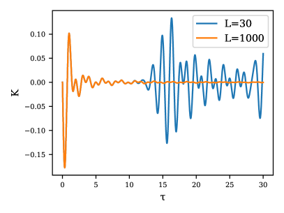
Figure 1. Time response function $K_{L}(\tau).$

We plot in Figure 1 the response function $K_{L}(\tau)$ for different values of $L$. Since $V_{\mathcal{O}}=V_{\mathcal{P}}$ and the spectrum of $H$ is continuous except for the single bound state, the exact response function $K(\tau)$ decays to zero, as the initial disturbance propagates to infinity. However when observed on a finite-sized box for long times, spurious reflections at the boundary introduce non-decaying oscillations.

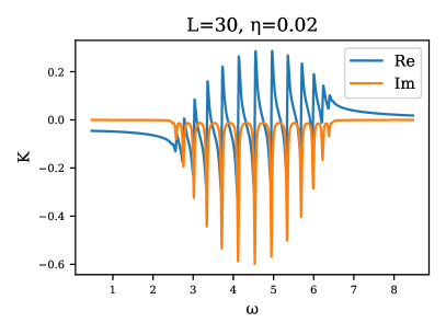
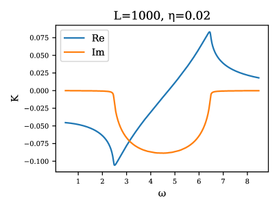
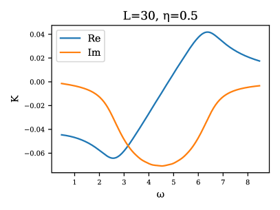
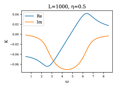
Figure 2. Frequency response function $\widehat{K}_{L}(\omega+i\eta)$.

This same phenomenon can be seen in frequency space in Figure 2, where we plot the frequency response function $\widehat{K}_{L}(\omega+i\eta)$ for different values of $\eta$ and $L$. We plot the region $\omega\in[0,9]$, which contains the region $[-2,2]-E_{0}$ corresponding to ionization; not represented is the other ionization region $E_{0}-[-2,2]$. When $\eta$ is small and $L\ll 1/\eta$, the discrete nature of the spectrum is evident, and the response function is composed of individual peaks. When $L\gg 1/\eta$, these peaks are blurred into a continuous function. Higher $\eta$ result in more accurate functions at moderate $L$, at the price of over-smoothing.

5. The Kubo formula

We begin by studying the eigenfunction $\psi_{0}$ associated to the eigenvalue $E_{0}$.

Lemma 5.1.

There is $\alpha_{0}>0$ such that $\psi_{0}\in H^{2}(e^{\alpha_{0}\langle x\rangle})$.

Proof.

Since $V$ decays at infinity, for all $\varepsilon>0$, we can write $V=V_{c}+V_{\varepsilon}$ with $V_{c}$ compactly supported and $\|V_{\varepsilon}\|_{L^{\infty}(\mathbb{R}^{d})}\leq\varepsilon$. Then, for $\varepsilon\leq-E_{0}/2$ we can write

$$\psi_{0}=-(-\Delta+V_{\varepsilon}-E_{0})^{-1}V_{c}\psi_{0}.$$

Since $V_{c}$ is compactly supported, $V_{c}\psi_{0}$ is in $L^{2}(e^{\alpha\langle x\rangle})$ for all $\alpha>0$, and so by Lemma 9.2, $\psi_{0}$ belongs to $H^{2}(e^{\alpha_{0}\langle x\rangle})$ for some $\alpha_{0}>0$ small enough. ∎

Note that this estimate is not sharp since the actual decay rate of $\psi_{0}$ is $\sqrt{-E_{0}}$ (which can be obtained by sharper Combes-Thomas estimates), but this will be sufficient for our purposes.

We now prove Kubo’s formula.

Proof of Theorem 3.1.

Let $U_{0}(t,s)=e^{-iH(t-s)}$ be the unitary propagator of the unperturbed Hamiltonian $H=-\Delta+V$, and $U_{\varepsilon}(t,s)$ that of the perturbed Hamiltonian $H_{\varepsilon}(t)=-\Delta+V+\varepsilon f(t)V_{\mathcal{P}}$, whose existence is guaranteed by Lemma 9.1. By the Duhamel/variation of constant formula,

$$\psi(t) =\underbrace{e^{-iE_{0}t}\psi_{0}}_{\psi^{0,0}(t)}\;\underbrace{-i\varepsilon\int_{0}^{t}U_{0}(t,t^{\prime})f(t^{\prime})V_{\mathcal{P}}U_{\varepsilon}(t^{\prime},0)\psi_{0}dt^{\prime}}_{\varepsilon\psi^{1,\varepsilon}(t)}.$$

Iterating this formula, we obtain the first-order Dyson expansion

$$\psi^{1,\varepsilon}(t)=\underbrace{-i\int_{0}^{t}f(t^{\prime})U_{0}(t,t^{\prime})V_{\mathcal{P}}U_{0}(t^{\prime},0)\psi_{0}dt^{\prime}}_{\psi^{1,0}(t)}\;\underbrace{-\varepsilon\int_{0}^{t}\int_{0}^{t^{\prime}}U_{0}(t,t^{\prime})f(t^{\prime})V_{\mathcal{P}}U_{0}(t^{\prime},t^{\prime\prime})f(t^{\prime\prime})V_{\mathcal{P}}U_{\varepsilon}(t^{\prime\prime},0)\psi_{0}dt^{\prime}dt^{\prime\prime}}_{\varepsilon\psi^{2,\varepsilon}(t)}.$$

From $\psi(t)=\psi^{0,0}(t)+\varepsilon\psi^{1,0}(t)+\varepsilon^{2}\psi^{2,\varepsilon}(t)$ it follows that

$$\langle\psi(t),V_{\mathcal{O}}\psi(t)\rangle =\langle\psi_{0},V_{\mathcal{O}}\psi_{0}\rangle+\varepsilon\Big{(}\langle\psi^{1,0}(t),V_{\mathcal{O}}\psi^{0,0}(t)\rangle+\langle\psi^{0,0}(t),V_{\mathcal{O}}\psi^{1,0}(t)\rangle\Big{)}$$

$$+\underbrace{\varepsilon^{2}\Big{(}\langle\psi^{2,\varepsilon}(t),V_{\mathcal{O}}\psi^{0,0}(t)\rangle+\langle\psi^{0,0}(t),V_{\mathcal{O}}\psi^{2,\varepsilon}\rangle+2\langle\psi^{1,0}(t),V_{\mathcal{O}}\psi^{1,0}(t)\rangle\Big{)}}_{R_{\varepsilon}(t)}$$

The first-order term can be computed as

$$\langle\psi^{0,0}(t),V_{\mathcal{O}}\psi^{1,0}(t)\rangle+{\rm c.c.} =\left\langle e^{iE_{0}t}V_{\mathcal{O}}\psi_{0},-i\int_{0}^{t}f(t^{\prime})e^{-iH(t-t^{\prime})}V_{\mathcal{P}}e^{-iE_{0}t^{\prime}}\psi_{0}dt^{\prime}\right\rangle+{\rm c.c.}$$

$$=-i\int_{0}^{t}f(t^{\prime})\langle V_{\mathcal{O}}\psi_{0},e^{-i(H-E_{0})(t-t^{\prime})}V_{\mathcal{P}}\psi_{0}\rangle dt^{\prime}+{\rm c.c.}.$$

$$=(K\ast f)(t).$$

Since $|V_{\mathcal{O}}(x)|\lesssim 1+|x|$ and $\psi_{0}\in L^{2}(e^{\alpha_{0}\langle x\rangle})$,

$$|R_{\varepsilon}(t)|\lesssim\|\psi^{2,\varepsilon}(t)\|+\|(1+|x|)\psi^{1,0}(t)\|.$$

Using $|V_{\mathcal{P}}(x)|\lesssim 1+|x|$ and Lemma 9.1, we get

$$\|\psi^{2,\varepsilon}(t)\| \lesssim(1+|t|^{2})\sup_{t^{\prime}\in[0,t],t^{\prime\prime}\in[0,t]}\|U_{0}(t,t^{\prime})V_{\mathcal{P}}U_{0}(t^{\prime},t^{\prime\prime})V_{\mathcal{P}}U_{\varepsilon}(t^{\prime\prime},0)\psi_{0}\|$$

$$\lesssim(1+|t|^{2})\sup_{t^{\prime}\in[0,t],t^{\prime\prime}\in[0,t]}\|(1+|x|)U_{0}(t^{\prime},t^{\prime\prime})V_{\mathcal{P}}U_{\varepsilon}(t^{\prime\prime},0)\psi_{0}\|$$

$$\lesssim(1+|t|^{4})\sup_{t^{\prime\prime}\in[0,t]}\Big{(}\|(1+|x|)V_{\mathcal{P}}U_{\varepsilon}(t^{\prime\prime},0)\psi_{0}\|+\|\nabla(V_{\mathcal{P}}U_{\varepsilon}(t^{\prime\prime},0)\psi_{0})\|\Big{)}$$

$$\lesssim(1+|t|^{4})\sup_{t^{\prime\prime}\in[0,t]}\Big{(}\||x|^{2}U_{\varepsilon}(t^{\prime\prime},0)\psi_{0}\|+\|\nabla U_{\varepsilon}(t^{\prime\prime},0)\psi_{0}\|+\|\psi_{0}\|\Big{)}$$

$$\lesssim(1+|t|^{8})\left(\||x|^{2}\psi_{0}\|+\|\Delta\psi_{0}\|+\|x\otimes\nabla\psi_{0}\|+\|\psi_{0}\|\right)$$

The bound on $R_{\varepsilon}(t)$ then follows by establishing a bound on $\|(1+|x|)\psi^{1,0}(t)\|$ by the same method. ∎

6. Properties of the response function $K$

Theorem 3.2 is a consequence of a limiting absorption principle for the Hamiltonian $H=-\Delta+V$ stated in Proposition 6.2. Our proof is a simplification of the one in Agmon [1], with a careful tracking of the regularity with respect to the spectral parameter.

We begin by studying the free Laplacian.

Proposition 6.1 (Limiting absorption principle for the free Laplacian).

Let $s=\tfrac{1}{2}+k+\alpha$ for $k\in\mathbb{N}$ and $\alpha\in[0,1]$. The resolvent $(z+\Delta)^{-1}$ defined for ${\rm Im}z>0$ extends to an operator of class $C^{k,\alpha}$ on the semi-open set $(0,+\infty)+i[0,+\infty)$, in the topology of bounded operators from $L^{2}\left(\langle x\rangle^{s}\right)$ to $H^{2}\left(\langle x\rangle^{-s}\right)$.

Proof.

Let $\lambda_{0}>0.$ Let $\chi$ be a smooth cutoff function, equal to $1$ in $[\lambda_{0}/2,2\lambda_{0}]$ and to zero outside of $[\lambda_{0}/3,3\lambda_{0}]$. Let $\psi\in L^{2}(\langle x\rangle^{s})$, and $\phi$ belong to the $L^{2}$-dual of $H^{2}\left(\langle x\rangle^{-s}\right)$.

Let $M_{\chi}$ be the multiplication operator in Fourier space defined by $\mathcal{F}(M_{\chi}\psi)(q)=\chi(|q|^{2})\mathcal{F}(q)$. Then by spectral calculus, $(z+\Delta)^{-1}(1-M_{\chi})$ extends to a $C^{k,\alpha}$ operator on a set $[\lambda_{0}-\varepsilon,\lambda_{0}+\varepsilon]+i[0,+\infty)$ for $\varepsilon$ small enough, in the topology of operators $L^{2}(\mathbb{R}^{d})$ to $H^{2}(\mathbb{R}^{d})$. Therefore, it is enough to consider the term

$$\langle\phi,(z+\Delta)^{-1}M_{\chi}\psi\rangle =\frac{1}{(2\pi)^{d}}\int_{\mathbb{R}^{d}}\frac{\chi\left(|q|^{2}\right)\mathcal{F}\phi(q)^{*}\mathcal{F}\psi(q)}{z-|q|^{2}}\mathrm{d}q$$

(11) $$=\int_{\mathbb{R}}\frac{D_{\phi\psi}(\lambda)}{z-\lambda}\mathrm{d}\lambda,$$

with the projected density of states

$$D_{\phi\psi}(\lambda)=\frac{1}{(2\pi)^{d}}\lambda^{(d-2)/2}\chi\left(\lambda\right)\int_{S^{d-1}}\mathcal{F}\phi(\sqrt{\lambda}\hat{q})^{*}\mathcal{F}\psi(\sqrt{\lambda}\hat{q})\mathrm{d}\hat{q}.$$

Since $\mathcal{F}(M_{\sqrt{\chi}}\phi)$ and $\mathcal{F}(M_{\sqrt{\chi}}\psi)$ are in $H^{s}(\mathbb{R}^{d})$, by Lemma 8.2 $D_{\phi\psi}$ is in $H^{s}(\mathbb{R})$.

We can compute by contour integration the inverse Fourier transform of the function $\frac{1}{z-\cdot}$ for ${\rm Im}z>0$:

$$\frac{1}{2\pi}\int\frac{1}{z-\lambda}e^{-i\lambda\tau}\mathrm{d}\lambda=i\theta(-\tau)e^{-iz\tau}$$

Therefore, by the Parseval formula,

$$\langle\phi,(z+\Delta)^{-1}M_{\chi}\psi\rangle=2\pi i\int_{\mathbb{R}^{+}}e^{iz\tau}\widecheck{D}_{\phi\psi}(\tau)\mathrm{d}\tau.$$

Letting $g_{\tau}(z)=e^{iz\tau}$, it follows from

$$|g_{\tau}^{(k)}(z_{1})-g_{\tau}^{(k)}(z_{2})|\lesssim|z_{1}-z_{2}|^{\alpha}|\tau|^{k+\alpha}$$

and the Cauchy-Schwarz inequality that $\langle\phi,(z-\Delta)^{-1}M_{\chi}\psi\rangle$ is $C^{k,\alpha}$ on $(0,+\infty)+i[0,+\infty)$. ∎

For $\lambda>0$, we denote by

$$(\lambda+i0^{+}+\Delta)^{-1}=\lim_{\eta\to 0^{+}}(\lambda+i\eta+\Delta)^{-1}$$

the boundary value of the free resolvent. Its action can be explicitly computed using the spectral representation (11) and the Plemelj-Sokhotski formula (5). Note in particular that it differs from $(\lambda+i0^{-}+\Delta)^{-1}$ by the sign of its anti-hermitian part.

Proposition 6.2 (Limiting absorption principle for $H=-\Delta+V$).

Let $s=\tfrac{1}{2}+k+\alpha$ for $k\in\mathbb{N}$ and $\alpha\in[0,1]$. Let $V:\mathbb{R}^{d}\to\mathbb{R}$ be a continuous potential such that $\langle x\rangle^{2s+\epsilon}V$ is bounded, for some $\varepsilon>0$. The resolvent $(z-H)^{-1}$ defined for ${\rm Im}z>0$ extends to an operator of class $C^{k,\alpha}$ on the semi-open set $(0,+\infty)+i[0,+\infty)$, in the topology of bounded operators from $L^{2}\left(\langle x\rangle^{s}\right)$ to $H^{2}\left(\langle x\rangle^{-s}\right)$.

Proof.

We use the following resolvent inequality:

(12) $$(z-H)^{-1}=B(z)^{-1}(z+\Delta)^{-1}$$

with

$$B(z)=1-(z+\Delta)^{-1}V,$$

valid for $z\in\mathbb{C}$ with ${\rm Im}z>0$. Since $V$ is bounded from $H^{2}(\langle x\rangle^{-s})$ to $L^{2}(\langle x\rangle^{s})$, it follows from Proposition 6.1 that $B(z)$ extends to an operator of class $C^{k,\alpha}$ on the semi-open set $(0,+\infty)+i[0,+\infty)$, in the topology of bounded operators on $H^{2}\left(\langle x\rangle^{-s}\right)$.

We will show that for all $\lambda>0$, $B(\lambda+i0^{+})$ is invertible on $H^{2}\left(\langle x\rangle^{-s}\right)$. This shows that $B(z)^{-1}$ is $C^{k,\alpha}$ on the semi-open set in the topology of bounded operators on $H^{2}\left(\langle x\rangle^{-s}\right)$, which implies our result by (12) and Proposition 6.1.

Let $\lambda>0$. Since $\langle x\rangle^{2s+\varepsilon}V$ is bounded, the multiplication operator $V$ is compact from $H^{2}(\langle x\rangle^{-s})$ to $L^{2}(\langle x\rangle^{s})$. It follows that $(\lambda+i0^{+}+\Delta)^{-1}V$ is compact on $H^{2}\left(\langle x\rangle^{-s}\right)$. By the Fredholm alternative, it is then enough to show that there are no non-zero solutions of

$$u=(\lambda+i0^{+}+\Delta)^{-1}Vu$$

in $H^{2}\left(\langle x\rangle^{-s}\right)$. Let $u\in H^{2}\left(\langle x\rangle^{-s}\right)$ be such a non-zero solution. Testing this equality against $Vu$ and taking imaginary parts, we obtain from the Plemelj-Sokhotski formula (5) that

$$0=\operatorname*{Im}(\langle Vu,u\rangle)={\rm Im}\langle Vu,(\lambda+i0^{+}+\Delta)^{-1}Vu\rangle=-\frac{\pi}{2\sqrt{\lambda}}\int_{|q|=\sqrt{\lambda}}|\mathcal{F}(Vu)(q)|^{2}\,\mathrm{d}q.$$

By Lemma 8.2,

$$\mathcal{F}u(q)=\frac{\mathcal{F}(Vu)(q)}{\lambda-|q|^{2}}$$

with $\mathcal{F}(Vu)\in H^{s}(\mathbb{R}^{d})$ shows that $\langle q\rangle^{2}\mathcal{F}u(q)\in H^{s-1}(\mathbb{R}^{d})$, and so that $u\in H^{2}(\langle x\rangle^{s-1})$. More generally, the argument above shows that if $u\in L^{2}(\langle x\rangle^{s^{\prime}})$ with $s^{\prime}\geq-s$, then $u\in H^{2}(\langle x\rangle^{s^{\prime}+2s-1})$, and, since $s>\tfrac{1}{2}$, it follows that $u\in H^{2}(\mathbb{R}^{d})$, and therefore that $\lambda$ is a positive embedded eigenvalue, which is impossible. ∎

Proof of Theorem 3.2.

By Theorem 3.1, the response function is given by

(13) $$\widehat{K}(\omega)=\lim_{\eta\to 0^{+}}\left\langle\psi_{0},V_{\mathcal{O}}\Big{(}\omega+i\eta-(H-E_{0})\Big{)}^{-1}V_{\mathcal{P}}\psi_{0}\right\rangle-\left\langle\psi_{0},V_{\mathcal{P}}\Big{(}\omega+i\eta+(H-E_{0})\Big{)}^{-1}V_{\mathcal{O}}\psi_{0}\right\rangle.$$

By the exponential localization of the ground state wave function $\psi_{0}$, and the assumptions on the potentials $V_{\mathcal{O}}$ and $V_{\mathcal{P}}$, $V_{\mathcal{O}}\psi_{0}$ and $V_{\mathcal{P}}\psi_{0}$ belong to every $L^{2}(\langle x\rangle^{s})$ for $s\in\mathbb{R}$. Since by Assumption 2.2 the function $\langle x\rangle^{2+\epsilon}V$ is bounded, the result follows by Proposition 6.2 in the case $k=0,\alpha=1$. ∎

7. Truncation in space

Consider the domain $\Omega_{L}=[-L,L]^{d}$ with Dirichlet boundary conditions. We define $\widetilde{H}_{L}$ the operator $-\Delta+V$ with domain $D(\widetilde{H}_{L})=\{\widetilde{\psi}\in H^{2}(\Omega_{L}),\widetilde{\psi}|_{\partial\Omega_{L}}=0\}$, self-adjoint on $L^{2}(\Omega_{L})$. This operator is bounded from below and has compact resolvent.

We now define the operator $H_{L}$ on $L^{2}(\mathbb{R}^{d})$ in the following way: if $\psi\in L^{2}(\mathbb{R}^{d})$ and $\psi|_{\Omega_{L}}\in D(\widetilde{H}_{L})$, then

$$({H_{L}}\psi)|_{\Omega_{L}}=\widetilde{H}_{L}\psi|_{\Omega_{L}},$$

and $({H_{L}}\psi)|_{\mathbb{R}^{d}\setminus\Omega_{L}}=0$. This defines an operator on $L^{2}(\mathbb{R}^{d})$, self-adjoint with domain $D(H_{L})=L^{2}(\mathbb{R}^{d}\setminus\Omega_{L})\oplus D(\widetilde{H}_{L})$, and with spectrum $\sigma(\widetilde{H}_{L})\cup\{0\}$. Let $\psi_{0,L}$ be an $L^{2}$-normalized eigenvector associated to the lowest eigenvalue of $H_{L}$.

Note that by adapting the proof in Lemma 9.1, the estimates shown there for $e^{-itH}$ on $L^{2}(\mathbb{R}^{d})$ are also valid for $e^{-it\widetilde{H}_{L}}$ on $L^{2}(\Omega_{L})$, with constants independent of $L$. Similarly, the estimates of Lemma 9.2 for $(z-H)^{-1}$ on $L^{2}(\mathbb{R}^{d})$ and $L^{2}(e^{\alpha\langle x\rangle})$ are also valid for $(z-\widetilde{H}_{L})^{-1}$ on $L^{2}(\Omega_{L})$ and $L^{2}(e^{\alpha\langle x\rangle};\Omega_{L})=\{\psi,e^{\alpha\langle x\rangle}\psi\in L^{2}(\Omega_{L})\}$ with natural norms, still with constants independent of $L$.

We can now define $K_{L}$ analogously to $K$:

(14) $$K_{L}(\tau) =-i\theta(\tau)\left\langle V_{\mathcal{O}}\psi_{0,L},e^{-i(H_{L}-E_{0,L})\tau}V_{\mathcal{P}}\psi_{0,L}\right\rangle+{\rm c.c.},$$

and

(15) $$\widehat{K}_{L}(\omega)=\lim_{\eta\to 0^{+}} \left\langle\psi_{0,L},V_{\mathcal{O}}\Big{(}\omega+i\eta-(H_{L}-E_{0,L})\Big{)}^{-1}V_{\mathcal{P}}\psi_{0,L}\right\rangle$$

$$- \left\langle\psi_{0,L},V_{\mathcal{P}}\Big{(}\omega+i\eta+(H_{L}-E_{0,L})\Big{)}^{-1}V_{\mathcal{O}}\psi_{0,L}\right\rangle.$$

The operator $H$ and $H_{L}$ have the same action, but $H$ has domain $D(H)=H^{2}(\mathbb{R}^{d})$, whereas $H_{L}$ has domain $D(H_{L})=\{\psi\in L^{2}(\mathbb{R}^{d}),\psi|_{\Omega_{L}}\in H^{2}(\Omega_{L}),\psi|_{\partial\Omega_{L}}=0\}$. These different domains do not even share a common core, making the direct comparison of $K_{L}$ and $K$ difficult. However, we will prove and use the fact that, when evaluated on localized quantities, their resolvents

(16) $$R(z)=(z-H)^{-1},\quad R_{L}(z)=(z-H_{L})^{-1}$$

and propagators $e^{-iHt}$ and $e^{-iH_{L}t}$, both defined on $L^{2}(\mathbb{R}^{d})$, are close. To that end, we let $\chi:\mathbb{R}^{d}\to\mathbb{R}$ be a smooth truncation function equal to $1$ for $|x|_{\infty}\leq 1/4$ and to 0 for $|x|_{\infty}\geq 3/4$, and

$$\chi_{L}(x)=\chi(x/L).$$

Note that, as a multiplication operator, $\chi_{L}$ maps $D(H)\cup D(H_{L})$ to $D(H)\cap D(H_{L})$.

Furthermore, this truncation is exponentially accurate on exponentially localized functions: by direct computation, for all $k\in\mathbb{N}$ there is $C_{k}>0$ such that, for all $0\leq\alpha_{1}\leq\alpha_{2}\leq 1$, for all $\psi\in H^{k}(e^{\alpha_{2}\langle x\rangle})$

$$\|(1-\chi_{L})\psi\|_{H^{k}(e^{\alpha_{1}\langle x\rangle})}=\|e^{(\alpha_{1}-\alpha_{2})\langle x\rangle}(1-\chi_{L})e^{\alpha_{2}\langle x\rangle}\psi\|_{H^{k}(\mathbb{R}^{d})}\leq C_{k}e^{-(\alpha_{2}-\alpha_{1})L}\|\psi\|_{H^{k}(e^{\alpha_{2}\langle x\rangle})}.$$

Lemma 7.1.

There are $c>0,C>0$ such that, for all $z\in\mathbb{C}$ and $L>0$ such that $d(K,\sigma(H))\geq g$ and $\liminf d(K,\sigma(H_{L}))\geq g$ with $g>0$, for all $0\leq\alpha\leq\alpha^{\prime}\leq cg$,

$$\|R_{L}(z)-R(z)\|_{L^{2}(e^{\alpha^{\prime}\langle x\rangle})\to L^{2}(e^{\alpha\langle x\rangle})}\leq C\left(1+\frac{1}{g}\right)^{2}(1+|z|)^{3}e^{-(\alpha^{\prime}-\alpha)L}.$$

Proof.

Because of the aforementioned domain issues, we cannot directly use the resolvent formula $R(z)-R_{L}(z)=R_{L}(z)(H-H_{L})R(z)$. However, we can approximate any $\psi\in L^{2}(\mathbb{R}^{d})$ by $R(z)^{-1}\chi_{L}R(z)\psi$, for which

$$(R(z)-R_{L}(z))\,R(z)^{-1}\chi_{L}R(z)\psi=R_{L}(z)(H-H_{L})\chi_{L}R(z)\psi=0,$$

where we have used that $H\phi=H_{L}\phi$ for all $\phi\in D(H_{L})\cap D(H)$. Therefore, using the estimates of Lemma 9.2 for both $H$ and $H_{L}$,

$$\|(R(z)-R_{L}(z))\psi\|_{L^{2}(e^{\alpha\langle x\rangle})} =\|(R(z)-R_{L}(z))(R(z)^{-1}(1-\chi_{L})R(z)\psi)\|_{L^{2}(e^{\alpha\langle x\rangle})}$$

$$\lesssim\left(1+\frac{1}{d(z,\sigma(H))}+\frac{1}{d(z,\sigma(H_{L}))}\right)(1+|z|)\|R(z)^{-1}(1-\chi_{L})R(z)\psi\|_{L^{2}(e^{\alpha\langle x\rangle})}$$

$$\lesssim\left(1+\frac{1}{d(z,\sigma(H))}+\frac{1}{d(z,\sigma(H_{L}))}\right)(1+|z|)^{2}\|(1-\chi_{L})R(z)\psi\|_{H^{2}(e^{\alpha\langle x\rangle})}$$

$$\lesssim\left(1+\frac{1}{d(z,\sigma(H))}+\frac{1}{d(z,\sigma(H_{L}))}\right)^{2}(1+|z|)^{3}e^{-(\alpha^{\prime}-\alpha)L}\|\psi\|_{L^{2}(e^{\alpha^{\prime}\langle x\rangle})}.$$

∎

Using this we can compare the eigenpairs of $H_{L}$ and $H$.

Lemma 7.2.

There are $C,\alpha_{1},\alpha_{2}>0$ such that, for all $L$ large enough,

(17) $$|E_{0,L}-E_{0}| \leq Ce^{-\alpha_{0}L}$$

(18) $$\|{\psi_{0,L}}-\psi_{0}\|_{L^{2}(e^{\alpha_{1}\langle x\rangle})} \leq Ce^{-\alpha_{2}L}$$

where the sign of $\psi_{0,L}$ is chosen such that $\langle{\psi_{0,L}},\psi_{0}\rangle\geq 0$, and where $\alpha_{0}$ is the constant in Lemma 5.1.

Proof.

Since by Lemma 5.1 $\psi_{0}\in H^{2}(e^{\alpha_{0}\langle x\rangle})$,

$$\|(1-\chi_{L})\psi_{0}\|_{H^{2}(\mathbb{R}^{d})}\lesssim e^{-\alpha_{0}L}.$$

and (17) follows from the variational principle

$$E_{0}\leq E_{0,L}\leq\frac{\langle\chi_{L}\psi_{0},H\chi_{L}\psi_{0}\rangle_{L^{2}(\mathbb{R}^{d})}}{\langle\chi_{L}\psi_{0},\chi_{L}\psi_{0}\rangle_{L^{2}(\mathbb{R}^{d})}}\leq E_{0}+Ce^{-\alpha_{0}L}.$$

for some $C>0$.

Let $E_{1,L}$ and $E_{1}$ be the second-lowest eigenvalue (or zero if there are no second eigenvalue) of $H_{L}$ and $H$ respectively. From the min-max principle, $E_{1,L}\geq E_{1}$ and therefore for $L$ large enough there is a gap $g>0$ in $\sigma(H_{L})$ above $E_{0,L}$. Let $C$ be the circle with center $E_{0}$ and radius $g/2$ in the complex plane, oriented trigonometrically. Then, by Lemma 7.1 there is $\alpha_{2}>0$ such that

$$1-\langle\psi_{0},\psi_{0,L}\rangle^{2} =\left\langle\psi_{0},\Big{(}|\psi_{0}\rangle\langle\psi_{0}|-|\psi_{0,L}\rangle\langle\psi_{0,L}|\Big{)}\psi_{0}\right\rangle$$

$$=\frac{1}{2\pi i}\oint_{\mathcal{C}}\left\langle\psi_{0},(R(z)-R_{L}(z))\psi_{0}\right\rangle dz$$

$$|1-\langle\psi_{0},\psi_{0,L}\rangle^{2}| \lesssim e^{-\alpha_{2}L}$$

Then

$$\frac{1}{2}\|\psi_{0}-\psi_{0,L}\|^{2}_{L^{2}(\mathbb{R}^{d})}=1-\langle\psi_{0},\psi_{0,L}\rangle=1-\sqrt{\langle\psi_{0},\psi_{0,L}\rangle^{2}}\lesssim e^{-\alpha_{2}L}.$$

Now, as in Lemma 5.1, let $V=V_{\varepsilon}+V_{c}$ with $V_{c}$ compactly supported and $\|V_{\varepsilon}\|_{L^{\infty}(\mathbb{R}^{d})}\leq-E_{0}/2$. Let $H_{L,\varepsilon}=-\Delta+V_{\varepsilon}$ on $\Omega_{L}$, extended as before to act on $L^{2}(\Omega)$. For $L$ large enough so that the support of $V_{c}$ is contained in $\Omega_{L}$, we have

$$\psi_{0,L} =(E_{0,L}-H_{L,\varepsilon})^{-1}V_{c}\psi_{0,L}.$$

Arguing as in Lemma 7.1, there are $\alpha_{1},\alpha^{\prime}>0$ such that $(E_{0,L}-H_{L,\varepsilon})^{-1}$ converges exponentially quickly to $(E_{0}-H)^{-1}$ as an operator from $L^{2}(e^{\alpha^{\prime}\langle x\rangle})$ to $L^{2}(e^{\alpha_{1}\langle x\rangle})$. Furthermore, because $V_{c}$ is compactly supported, we have

$$\|V_{c}\psi_{0,L}-V_{c}\psi_{0}\|_{L^{2}(e^{\alpha^{\prime}\langle x\rangle})}\lesssim\|\psi_{0,L}-\psi_{0}\|_{L^{2}(\mathbb{R}^{d})}\lesssim e^{-\alpha_{2}L}$$

and the result follows. ∎

With this we can now prove the convergence of $K_{L}(\omega+i\eta)$ for positive $\eta$.

Theorem 7.3.

There are $\alpha_{3}>0,C>0$ such that for all $0<\eta<1$, $\omega\in\mathbb{R}$,

$$|\widehat{K}_{L}(\omega+i\eta)-\widehat{K}(\omega+i\eta)|\leq\frac{C(1+\omega)^{3}}{\eta^{2}}e^{-\alpha_{3}\eta L}$$

Proof.

Since $\psi_{0,L}$ converges exponentially towards $\psi_{0}$ in $L^{2}(e^{\alpha\langle x\rangle})$ for some $\alpha>0$, and $V_{\mathcal{O}}$ and $V_{\mathcal{P}}$ have at most polynomial growth, $V_{\mathcal{O}}\psi_{0,L}$ and $V_{\mathcal{P}}\psi_{0,L}$ converge exponentially quickly in $L^{2}(\mathbb{R}^{d})$ towards $V_{\mathcal{O}}\psi_{0}$ and $V_{\mathcal{P}}\psi_{0}$ respectively. $E_{0,L}$ converges exponentially towards $E_{0}$ and $\Big{(}\omega+i\eta-(H_{L}-E_{0,L})\Big{)}^{-1}$ is uniformly bounded by $1/\eta$ as an operator on $L^{2}(\mathbb{R}^{d})$. It therefore follows that we can reduce to terms of the form

$$\left\langle\psi_{l},\Big{(}R_{L}(\omega-E_{0}+i\eta)-R(\omega-E_{0}+i\eta)\Big{)}\psi_{r}\right\rangle$$

with $\psi_{l/r}\in L^{2}(e^{\alpha\langle x\rangle})$ for some $\alpha>0$ independent on $\omega,\eta$. We can then conclude using Lemma 7.1. ∎

Finally, we conclude the proof of Theorem 3.3.

Theorem 7.4.

$K_{L}$ converges as a tempered distribution towards $K$.

Proof.

We will prove that, for all $f\in\mathcal{S}(\mathbb{R})$,

$$\int_{0}^{\infty}\left\langle V_{\mathcal{O}}\psi_{0,L},e^{-i(H_{L}-E_{0,L})t}V_{\mathcal{P}}\psi_{0,L}\right\rangle f(t)dt\rightarrow\int_{0}^{\infty}\left\langle V_{\mathcal{O}}\psi_{0},e^{-i(H-E_{0})t}V_{\mathcal{P}}\psi_{0}\right\rangle f(t)dt.$$

Since $\psi_{0,L}\to\psi_{0}$ in $H^{2}(e^{\alpha_{1}\langle x\rangle})$,

$$\|V_{\mathcal{O}}\psi_{0,L}-\chi_{L}V_{\mathcal{O}}\psi_{0}\|\to 0$$

and similarly for $V_{\mathcal{P}}$. It is therefore sufficient to prove that

$$\|\chi_{L}(e^{-iHt}-e^{-iH_{L}t})\chi_{L}V_{\mathcal{P}}\psi_{0}\|\leq\frac{P(t)}{L}$$

for some polynomial $P$. Let

$$\phi(t)=e^{-iHt}\chi_{L}V_{\mathcal{P}}\psi_{0},\quad\phi_{L}(t)=e^{-iH_{L}t}\chi_{L}V_{\mathcal{P}}\psi_{0}$$

To estimate $\chi_{L}(\phi(t)-\phi_{L}(t))$ we compute

$$i\partial_{t}\chi_{L}(\phi-\phi_{L}) =H\chi_{L}\phi-H_{L}\chi_{L}\phi_{L}+[\chi_{L},H]\phi-[\chi_{L},H_{L}]\phi_{L}$$

$$=H\chi_{L}(\phi-\phi_{L})+[\chi_{L},H]\phi-[\chi_{L},H_{L}]\phi_{L}$$

and therefore by the Duhamel formula

$$\chi_{L}(\phi(t)-\phi_{L}(t)) =-i\int_{0}^{t}e^{-iH(t-t^{\prime})}\left([\chi_{L},H]\phi(t^{\prime})-[\chi_{L},H_{L}]\phi_{L}(t^{\prime})\right)dt^{\prime}$$

$$\|\chi_{L}(\phi(t)-\phi_{L}(t))\| \leq t\sup_{t^{\prime}\in[0,t]}\left\|[\chi_{L},H]\phi(t^{\prime})-[\chi_{L},H_{L}]\phi_{L}(t^{\prime})\right\|.$$

Since $[\chi_{L},H]\phi=2\nabla\chi_{L}\cdot\nabla\phi+\Delta\chi_{L}\phi$ is zero for $|x|_{\infty}<L/4$, by Lemma 9.1 we have

$$\|[\chi_{L},H]\phi(t^{\prime})\| \lesssim\frac{1}{L}\|(1+|x|)[\chi_{L},H]\phi(t^{\prime})\|$$

$$\lesssim\frac{1}{L}\left(\|x\otimes\nabla\phi(t^{\prime})\|+\|\nabla\phi(t^{\prime})\|+\|(1+|x|)\phi(t^{\prime})\|\right)$$

$$\lesssim\frac{1+|t|^{4}}{L}$$

and similarly with $[\chi_{L},H_{L}]\phi_{L}(t^{\prime})$. The result follows. ∎

8. Appendix: trace theory in Sobolev spaces

We will need the following lemma on the regularity of traces on surfaces with respect to variations of the surface.

Lemma 8.1.

Let $\chi:\mathbb{R}\to\mathbb{R}$ be a smooth function with support $[R_{1},R_{2}]$, with $R_{1}>0$, and $s_{1},s_{2},s$ nonnegative real numbers such that $s_{1}+s_{2}=s$. Then for all $u\in H^{s}(\mathbb{R}^{d})$, the function

$$r\mapsto(\hat{x}\mapsto\chi(r)u(r\hat{x}))$$

is in $H^{s_{1}}(\mathbb{R},H^{s_{2}}(S^{d-1}))$.

Proof.

We first treat the case of the restriction to a hyperplane: if $u\in H^{s}(\mathbb{R}^{d})$, then

$$v_{u}:x_{1}\mapsto(x^{\prime}\mapsto u(x_{1},x^{\prime}))$$

is in $H^{s_{1}}(\mathbb{R},H^{s_{2}}(\mathbb{R}^{d-1}))$. Indeed, denoting for clarity by $\mathcal{F}_{1}$ the one-dimensional Fourier transform, we have by the Parseval formula on $L^{2}(\mathbb{R}^{d-1})$ that for all $q_{1}\in\mathbb{R}$,

$$\|\mathcal{F}_{1}v_{u}(q_{1})\|_{H^{s_{2}}(\mathbb{R}^{d-1})}^{2}=\frac{1}{(2\pi)^{d-1}}\int_{\mathbb{R}^{d-1}}\langle q^{\prime}\rangle^{2s_{2}}|\mathcal{F}u(q_{1},q^{\prime})|^{2}\mathrm{d}q^{\prime}$$

and therefore

$$\|v_{u}\|^{2}_{H^{s_{1}}(\mathbb{R},H^{s_{2}}(\mathbb{R}^{d-1}))}=\frac{1}{2\pi}\int_{\mathbb{R}}\langle q_{1}\rangle^{2s_{1}}\|\mathcal{F}_{1}v_{u}(q_{1})\|_{H^{s_{2}}(\mathbb{R}^{d-1})}^{2}\mathrm{d}q_{1}\leq\frac{1}{(2\pi)^{d}}\int_{\mathbb{R}^{d}}\langle q\rangle^{2s}|\mathcal{F}u(q)|^{2}\mathrm{d}q=\|u\|_{H^{s}(\mathbb{R}^{d})}^{2}.$$

To lift this property to the sphere $S^{d-1}(R)$ of radius $R$, we use a classical “flattening” argument. Using spherical coordinates, we can construct a cover of the annulus of inner radius $R_{1}$ and outer radius $R_{2}$ by open sets $\{X_{i}\}_{i=1,\dots,N}$ not touching zero with the property that, for every $i\in\{1,\dots,N\}$, there is a smooth diffeomorphism $\Phi_{i}$ from a an open set $\mathcal{R}_{i}\times\mathcal{T}_{i}\subset\mathbb{R}\times\mathbb{R}^{d-1}$ to $X_{i}$ such that, for all $(r,\theta)\in\mathcal{R}_{i}\times\mathcal{T}_{i}$,

$$\Phi_{i}(r,\theta)=r\,\Theta_{i}(\theta)$$

with $\Theta_{i}$ having values on the sphere $S^{d-1}$. One can then construct a partition of the unity $\zeta_{i}:\mathbb{R}^{d}\to\mathbb{R}$ where, for each $i\in\{1,\dots,N\}$, $\zeta_{i}$ is supported inside $X_{i}$, and $\sum_{i=1}^{N}\zeta_{i}=1$ on the annulus. Then, for all $u\in H^{s}(\mathbb{R}^{d})$, $|x|\in[R_{1},R_{2}]$,

$$\chi(|x|)u(x)=\sum_{i=1}^{N}\chi(|x|)\,\zeta_{i}(x)\,u(x)=\sum_{i,\;x\in X_{i}}w_{i}(\Phi_{i}^{-1}(x))$$

where

$$w_{i}(r,\theta)=\chi(r)\,\zeta_{i}(r\Theta_{i}(\theta))\,u(r\Theta_{i}(\theta)),$$

defined on $\mathcal{R}_{i}\times\mathcal{T}_{i}$, extends on the whole $\mathbb{R}^{d}$ to a $H^{s}(\mathbb{R}^{d})$ function. It follows from the hyperplane case that

$$\chi(r)u(r\hat{x})=\sum_{i,\;x\in X_{i}}w_{i}\left(r,\Theta_{i}^{-1}(\hat{x})\right)$$

is in $H^{s_{1}}(\mathbb{R},H^{s_{2}}(S^{d-1}))$. ∎

Note that from the fact that $H^{\frac{1}{2}+\varepsilon}(\mathbb{R})$, $\varepsilon>0$, functions are continuous, we recover the classical trace theorem that traces of $H^{s+\frac{1}{2}+\varepsilon}(\mathbb{R}^{d})$ functions are $H^{s}$ on surfaces.

The proof of the limiting absorption principle for the nonzero potential case requires the following Hardy-type inequality.

Lemma 8.2.

Let $s>0$, and $u\in H^{s}(\mathbb{R}^{d})$ such that $u$ is zero on the sphere of radius $a$ (in the sense of traces). Then the function $v(x)=\tfrac{u(x)}{|x|^{2}-a^{2}}$ is $H^{s-1}(\mathbb{R}^{d})$.

Proof.

Using as before a smooth cutoff function and a partition of unity of a neighborhood of the sphere of radius $a$, it is enough to show that for $u\in H^{s}(\mathbb{R}^{d})$ with $u(0,x^{\prime})=0$ for all $x^{\prime}\in\mathbb{R}^{d-1}$, then $v(x)=\tfrac{u(x)}{x_{1}}$ is $H^{s-1}(\mathbb{R}^{d-1})$.

Proceeding by density, we can assume that $\mathcal{F}u\in C^{\infty}_{c}(\mathbb{R}^{d})$. Then, using the fact that $\int\mathcal{F}u(q_{1},q^{\prime})\mathrm{d}q_{1}=0$ for all $q^{\prime}\in\mathbb{R}^{d-1}$, we have that $\mathcal{F}v\in C^{\infty}_{c}(\mathbb{R}^{d})$, and $\mathcal{F}u(q)=-i\tfrac{\partial\mathcal{F}v}{\partial q_{1}}(q)$. By integration by parts and the Cauchy-Schwarz inequality, we have the following Hardy inequality, for $q=(q_{1},q^{\prime})$ and $\alpha\in\mathbb{R}$:

$$\int_{\mathbb{R}}|\mathcal{F}v(q)|^{2}\langle q_{1}\rangle^{2(\alpha-1)}\,\mathrm{d}q_{1}\lesssim\int_{\mathbb{R}}|\mathcal{F}v(q)||\mathcal{F}u(q)|\langle q_{1}\rangle^{(\alpha-1)+\alpha}\,\mathrm{d}q_{1}\lesssim\int_{\mathbb{R}}{|\mathcal{F}u(q)|}^{2}\langle q_{1}\rangle^{2\alpha}\,\mathrm{d}q_{1}.$$

In the case $s\geq 1$, we have $\langle q\rangle^{2(s-1)}\lesssim\langle q_{1}\rangle^{2(s-1)}+\langle q^{\prime}\rangle^{2(s-1)}$ and so

$$\|v\|^{2}_{H^{s-1}} \lesssim\int_{\mathbb{R}^{d-1}}\int_{\mathbb{R}}|\mathcal{F}v(q)|^{2}\left(\langle q_{1}\rangle^{2(s-1)}+\langle q^{\prime}\rangle^{2(s-1)}\right)\,\mathrm{d}q_{1}\mathrm{d}q^{\prime}.$$

By using the Hardy inequality with $\alpha=s$ for the first term and $\alpha=1$ for the second, we get

$$\|v\|^{2}_{H^{s-1}} \lesssim\int_{\mathbb{R}^{d}}|\mathcal{F}u(q)|^{2}\langle q_{1}\rangle^{2s}\,\mathrm{d}q+\int_{\mathbb{R}^{d}}|\mathcal{F}u(q)|^{2}\langle q_{1}\rangle^{2}\langle q^{\prime}\rangle^{2(s-1)}\,\mathrm{d}q$$

$$\lesssim\int_{\mathbb{R}^{d}}|\mathcal{F}u(q)|^{2}\langle q\rangle^{2s}\,\mathrm{d}q\lesssim\|u\|_{H^{s}}^{2}.$$

In the case $0<s<1$, we have $\langle q\rangle^{2(s-1)}\leq\langle q_{1}\rangle^{2(s-1)}$ and we can repeat the above argument. ∎

9. Appendix: locality estimates on resolvents and propagators

We prove in this appendix results on the locality of the resolvents and propagators of Schrödinger operators. This appendix is independent from the rest of the paper.

Lemma 9.1 (Properties of the propagator).

Let $W:\mathbb{R}\times\mathbb{R}^{d}\to\mathbb{R}$ be a potential such that $W$ is continuous on $\mathbb{R}\times\mathbb{R}^{d}$ and for all $t\in\mathbb{R}$, $W(t,\cdot)$ is $C^{\infty}(\mathbb{R}^{d})$ and satisfies the sub-linear condition: for all $|\alpha|\geq 1$, $\partial_{x}^{\alpha}W$ is bounded on $\mathbb{R}\times\mathbb{R}^{d}$.

There exists a unitary propagator $U(t,s)$ such that if $\psi_{s}\in\mathcal{S}(\mathbb{R}^{d})$, $U(t,s)\psi_{s}\in\mathcal{S}(\mathbb{R}^{d})$ satisfies the Schrödinger equation

$$i\partial_{t}U(t,s)\psi_{s}=(-\Delta+W(t))U(t,s)\psi_{s}.$$

Furthermore, there is $C_{0}>0$ not depending on $W$ such that, for all $t,s\in\mathbb{R},\psi_{s}\in L^{2}(\mathbb{R}^{d})$,

(19) $$\|xU(t,s)\psi_{s}\|+\|\nabla U(t,s)\psi_{s}\| \leq C_{1}(t,s)\left(\|x\psi_{s}\|+\|\nabla\psi_{s}\|+\|\psi_{s}\|\right)$$

(20) $$\||x|^{2}U(t,s)\psi_{s}\|+\|\Delta U(t,s)\psi_{s}\| \leq C_{2}(t,s)\left(\||x|^{2}\psi_{s}\|+\|\Delta\psi_{s}\|+\|x\otimes\nabla\psi_{s}\|+\|\psi_{s}\|\right)$$

where

$$C_{1}(t,s) =C_{0}(1+|t-s|)^{2}\left(1+\sup_{t^{\prime}\in[t,s]}|\nabla W(t^{\prime})|\right)$$

$$C_{2}(t,s) =C_{0}(1+|t-s|)^{4}\left(1+\sup_{t^{\prime}\in[t,s]}|\nabla W(t^{\prime})|^{2}+\sup_{t^{\prime}\in[t,s]}|\nabla^{2}W(t^{\prime})|\right)$$

Note that these estimates are natural in the case $W=0$. In this case, $(\mathcal{F}\psi)(t,q)=(\mathcal{F}\psi)(s,q)e^{-i(t-s)|q|^{2}}$, and so $\partial_{q}(\mathcal{F}\psi)(t,q)=\partial_{q}(\mathcal{F}\psi)(s,q)e^{-i|q|^{2}(t-s)}-2iq(t-s)(\mathcal{F}\psi)(s,q)e^{-i|q|^{2}(t-s)}$, which is in $L^{2}(\mathbb{R}^{d})$ if $\psi_{s}\in L^{2}(\langle x\rangle)\cap H^{1}(\mathbb{R}^{d})$.

Proof.

The existence of the propagator is obtained using the results of [12] (which actually only requires a sub-quadratic potential).

We will obtain these inequalities by the following standard commutator method. Let $A$ be an operator, and $\psi_{s}\in L^{2}(\mathbb{R}^{d})$. Then, if $\psi(t)=U(t,s)\psi_{s}$, we have

$$i\partial_{t}(A\psi)(t^{\prime})=AH(t^{\prime})\psi(t^{\prime})=H(t^{\prime})A\psi(t^{\prime})+[A,H(t^{\prime})]\psi(t^{\prime})$$

and therefore by Duhamel’s formula,

$$A\psi(t)=U(t,s)A\psi(s)-i\int_{s}^{t}U(t,t^{\prime})[A,H(t^{\prime})]U(t^{\prime},s)dt^{\prime}.$$

We compute the following commutators

$$[\nabla,H(t)] =\nabla W(t)$$

$$[x,H(t)] =2\nabla$$

Since $\nabla W$ is a bounded operator, we obtain

$$\|\nabla U(t,s)\psi_{s}\| \leq\|\nabla\psi_{s}\|+|t-s|\sup_{t^{\prime}\in[s,t]}|\nabla W(t^{\prime})|\|\psi_{s}\|$$

$$\|xU(t,s)\psi_{s}\| \leq\|x\psi_{s}\|+2|t-s|\sup_{t^{\prime}\in[s,t]}\|\nabla U(t^{\prime},s)\psi_{s}\|$$

$$\leq\|x\psi_{s}\|+2|t-s|\left(\|\nabla\psi_{s}\|+|t-s|\sup_{t^{\prime}\in[s,t]}|\nabla W(t^{\prime})|\|\psi_{s}\|\right)$$

and (19) follows. Similarly, from the commutators

$$[\nabla^{2},H(t)] =\nabla^{2}W+2(\nabla W(t))\otimes\nabla$$

$$[x\otimes\nabla,H(t)] =-2\nabla^{2}+x\otimes\nabla W(t)$$

$$[x\otimes x,H(t)] =2x\otimes\nabla+2I$$

we obtain (20). ∎

Lemma 9.2 (Properties of the resolvent).

Let $W:\mathbb{R}^{d}\to\mathbb{R}$ be a bounded function, and $R(z)=(z-(-\Delta+W))^{-1}$. Then there are $c>0,C>0$ such that, for all $z\notin\sigma(H)$,

$$\|R(z)\|_{L^{2}(\mathbb{R}^{d})\to H^{2}(\mathbb{R}^{d})} \leq C(1+|z|)\left(1+\frac{1}{d(z,\sigma(H))}\right)$$

$$\|R(z)\|_{L^{2}(e^{\alpha\langle x\rangle})\to H^{2}(e^{\alpha\langle x\rangle})} \leq C(1+|z|)\left(1+\frac{1}{d(z,\sigma(H))}\right)\quad\forall\alpha\leq\alpha_{z}:=cd(z,\sigma(H))$$

Proof.

The first inequality is classical (see for instance [14] Lemma 3.6).

The second is a (non-sharp) Combes-Thomas estimate, which we prove for completeness here. Denote by

(21) $$H_{\alpha}:=e^{\alpha\langle x\rangle}(-\Delta+W)e^{-\alpha\langle x\rangle}=(-\Delta+W)+\underbrace{-2\alpha\nabla\langle x\rangle\cdot\nabla+\alpha^{2}\Delta(\langle x\rangle)}_{\alpha B_{\alpha}}.$$

Let $R(z)=(z-(-\Delta+W))^{-1}$. We have that

$$B_{\alpha}R(z)=(-2\nabla\langle x\rangle\cdot\nabla+\alpha\Delta(\langle x\rangle))(1-\Delta)^{-1}(1-\Delta)R(z)$$

is bounded as an operator on $L^{2}(\mathbb{R}^{d})$ by $C/d(z,\sigma(H))$, for all $\alpha\leq 1$, for some $C>0$. It follows that, for $\alpha\leq d(z,\sigma(H))/(2C)$

$$(z-H_{\alpha})^{-1}=R(z)(1+\alpha B_{\alpha}R(z))^{-1}$$

is bounded from $L^{2}(\mathbb{R}^{d})$ to $H^{2}(\mathbb{R}^{d})$ with norm smaller than $\frac{C^{\prime}}{d(z,\sigma(H))}$ for some $C^{\prime}>0$. Then, for all $\psi\in L^{2}(e^{\alpha\langle x\rangle})$,

$$\|R(z)\psi\|_{H^{2}(e^{\alpha\langle x\rangle})}=\|(z-H_{\alpha})^{-1}e^{\alpha\langle x\rangle}\psi\|_{H^{2}(\mathbb{R}^{d})}\leq\frac{C^{\prime}}{d(z,\sigma(H))}\|\psi\|_{L^{2}(e^{\alpha\langle x\rangle})}$$

∎

$*$ Faculty of Mathematics, Technische Universität München, Germany (dupuy@ma.tum.de)
$\dagger$ Inria Paris and Université Paris-Est, CERMICS, École des Ponts ParisTech, Marne-la-Vallée, France (antoine.levitt@inria.fr)

References

- [1] Shmuel Agmon “Spectral properties of Schrödinger operators and scattering theory” In Ann. Scuola Norm. Sup. Pisa Cl. Sci. (4) 2.2, 1975, pp. 151–218 URL: http://www.numdam.org/item?id=ASNSP_1975_4_2_2_151_0
- [2] Shmuel Agmon and Markus Klein “Analyticity properties in scattering and spectral theory for Schrödinger operators with long-range radial potentials” In Duke Math. J. 68.2, 1992, pp. 337–399 DOI: 10.1215/S0012-7094-92-06815-3
- [3] Xavier Antoine, Emmanuel Lorin and Qinglin Tang “A friendly review of absorbing boundary conditions and perfectly matched layers for classical and relativistic quantum waves equations” In Molecular Physics 115.15-16 Taylor & Francis, 2017, pp. 1861–1879
- [4] Sven Bachmann, Wojciech De Roeck and Martin Fraas “The adiabatic theorem and linear response theory for extended quantum systems” In Communications in Mathematical Physics 361.3 Springer, 2018, pp. 997–1027
- [5] Jean-Marc Bouclet, Francois Germinet, Abel Klein and Jeffrey H Schenker “Linear response theory for magnetic Schrödinger operators in disordered media” In Journal of Functional Analysis 226.2 Elsevier, 2005, pp. 301–372
- [6] Eric Cancès, Rachida Chakir and Yvon Maday “Numerical analysis of the planewave discretization of some orbital-free and Kohn-Sham models” In ESAIM: Mathematical Modelling and Numerical Analysis 46.2 EDP Sciences, 2012, pp. 341–388
- [7] Eric Cancès, Virginie Ehrlacher and Yvon Maday “Non-consistent approximations of self-adjoint eigenproblems: application to the supercell method” In Numerische Mathematik 128.4 Springer, 2014, pp. 663–706
- [8] Eric Cancès and Gabriel Stoltz “A mathematical formulation of the random phase approximation for crystals” In Annales de l’IHP Analyse non linéaire 29.6, 2012, pp. 887–925
- [9] Eric Cances et al. “Numerical quadrature in the Brillouin zone for periodic Schrödinger operators” In Numerische Mathematik 144.3 Springer, 2020, pp. 479–526
- [10] Eric Cancès, Clotilde Fermanian Kammerer, Antoine Levitt and Sami Siraj-Dine “Coherent electronic transport in periodic crystals” In arXiv preprint arXiv:2002.01990, 2020
- [11] Marco d’Alessandro and Luigi Genovese “Locality and computational reliability of linear response calculations for molecular systems” In Physical Review Materials 3.2 APS, 2019, pp. 023805
- [12] Daisuke Fujiwara “A construction of the fundamental solution for the Schrödinger equation” In Journal d’Analyse Mathématique 35.1 Springer, 1979, pp. 41–96
- [13] David Gontier and Salma Lahbabi “Supercell calculations in the reduced Hartree–Fock model for crystals with local defects” In Applied Mathematics Research eXpress 2017.1 Oxford University Press, 2017, pp. 1–64
- [14] Antoine Levitt “Screening in the Finite-Temperature Reduced Hartree–Fock Model” In Archive for Rational Mechanics and Analysis 238.2 Springer, 2020, pp. 901–927
- [15] JG Muga, JP Palao, B Navarro and IL Egusquiza “Complex absorbing potentials” In Physics Reports 395.6 Elsevier, 2004, pp. 357–426
- [16] Emil Prodan “Quantum transport in disordered systems under magnetic fields: A study based on operator algebras” In Applied Mathematics Research eXpress 2013.2 Oxford University Press, 2013, pp. 176–265
- [17] Maria Barbara Radosz “The principles of limit absorption and limit amplitude for periodic operators”, 2010
- [18] Michael Reed and Barry Simon “Methods of modern mathematical physics. III: Scattering theory” Elsevier, 1978
- [19] Michael Reed and Barry Simon “Methods of modern mathematical physics. IV: Analysis of operators” Elsevier, 1978
- [20] Plamen Stefanov “Approximating resonances with the complex absorbing potential method” In Communications in Partial Differential Equations 30.12 Taylor & Francis, 2005, pp. 1843–1862
- [21] Stefan Teufel “Non-equilibrium almost-stationary states and linear response for gapped quantum systems” In Communications in Mathematical Physics 373.2 Springer, 2020, pp. 621–653