Lorentzian path integral for quantum tunneling and WKB approximation
for wave-function

Abstract

Recently, the Lorentzian path integral formulation using the Picard-Lefschetz theory has attracted much attention in quantum cosmology. In this paper, we analyze the tunneling amplitude in quantum mechanics by using the Lorentzian Picard-Lefschetz formulation and compare it with the WKB analysis of the conventional Schrödinger equation. We show that the Picard-Lefschetz Lorentzian formulation is consistent with the WKB approximation for wave-function and the Euclidean path integral formulation utilizing the solutions of the Euclidean constraint equation. We also consider some problems of this Lorentzian Picard-Lefschetz formulation and discuss a simpler semiclassical approximation of the Lorentzian path integral without integrating the lapse function.

I Intorduction

Wave function distinguishes quantum and classical picture of physical systems and can be exactly calculated by solving the Schrödinger equation for quantum mechanics (QM). In particular, quantum tunneling is one of the most important consequences of the wave function. The wave function inside the potential barrier seeps out the barrier even if the kinetic energy is lower than the potential energy. As a result, the non-zero probability occurs outside the potential in the quantum system even if it is bound by the potential barrier in the classical system. Hence, quantum tunneling is one of the most important phenomena to describe the quantum nature of the system.

The Feynman’s path integral Feynman (1948) is a standard formulation for QM and quantum field theory (QFT) which is equivalent with Schrödinger equation and defines quantum transition amplitude which is given by the integral over all paths weighted by the factor $e^{iS[x]/\hbar}$. In the path integral formulation, the transition amplitude from an initial state $x(t_{i})=x_{i}$ to a final state $x(t_{f})=x_{f}$ is written by the functional integral,

$$K(x_{f};x_{i}) =\langle x_{f},t_{f}\mid x_{i},t_{i}\rangle$$

$$=\int_{x(t_{i})=x_{i}}^{x(t_{f})=x_{f}}\mathcal{D}x(t)\,\exp\left(\frac{iS[x]}{\hbar}\right),$$ (1)

where we consider a unit mass particle whose the action $S[x]$ is written by

$$S[x]=\int\mathrm{d}t\left(\frac{1}{2}\dot{x}^{2}-V(x)\right)\,.$$ (2)

In a semi-classical regime, the associated path integral can be given by the saddle point approximation which is dominated by the path $\delta S[x]/\delta x\approx 0$. In particular, to describe the quantum tunneling in Feynman’s formulation the Euclidean path integral method Coleman (1977) is used. Performing the Wick rotation $\tau=it$ to Euclidean time, the dominant field configuration is given by solutions of the Euclidean equations of motion imposed by boundary conditions. The instanton constructed by the half-bounce Euclidean solutions going from $x_{i}$ to $x_{f}$ Polyakov (1977) describes the tunneling event across a degenerate potential and the splitting energy. On the other hand, the bounce constructed by the bouncing Euclidean solutions with $x_{i}=x_{f}$ gives the vacuum decay ratio from the local-minimum false vacuum Coleman (1977). The Euclidean instanton method is useful tool for QFT Belavin et al. (1975); Polyakov (1977); Coleman (1977); Callan and Coleman (1977) and even the gravity Coleman and De Luccia (1980).

However, the method is conceptually less straightforward. When a particle tunnels through a potential barrier, we can accurately calculate the tunneling probability by using the Euclidean action $S_{E}[x]$ with the instanton solution, and in fact, it works well. However, when the particle is moving outside the potential, one needs to use the Lorentzian or real-time path integral so that the instanton formulation lacks unity and it is unclear why this method works. In this perspective, the quantum tunneling of the Lorentzian or real-time path integrals has been studied in recent years Levkov and Sibiryakov (2005); Bender, Brody, and Hook (2008); Bender (2009); Bender et al. (2010); Bender and Hook (2011); Dumlu and Dunne (2011); Turok (2014); Tanizaki and Koike (2014); Cherman and Unsal (2014); Behtash et al. (2016, 2017); Ilderton, Torgrimsson, and Wårdh (2015); Bramberger, Lavrelashvili, and Lehners (2016); Ai, Garbrecht, and Tamarit (2019), where complex instanton solutions are considered. It has been argued in Ref. Cherman and Unsal (2014); Ai, Garbrecht, and Tamarit (2019) that the Euclidean-time instanton solutions for a rotated time $t=\tau e^{-i\alpha}$ close to Lorentzian-time describes something like a real-time description of quantum tunneling. Besides the extensions of the instanton method, a new tunneling approach has been proposed by Ref. Feldbrugge, Lehners, and Turok (2017a) for quantum cosmology where the Lorentzian path integral includes a lapse integral and the saddle-point integration is performed by the Picard-Lefschetz theory (we call this method Lorentzian Picard-Lefschetz formulation). Feldbrugge et al. Feldbrugge, Lehners, and Turok (2017a) showed that the Lorentzian path integral reduces to the Vilenkin’s tunneling wave function Vilenkin (1984) by perfuming the integral over a contour. On other hand, Diaz Dorronsoro et al. reconsidered the Lorentzian path integral by integrating the lapse gauge over a different contour Diaz Dorronsoro et al. (2017) and show that the Lorentzian path integral reduces to be the Hartle-Hawking’s no boundary wave function Hartle and Hawking (1987). Both the tunneling or no-boundary wave functions can be derived as the Wentzel-Kramers-Brillouin (WKB) solutions of the Wheeler-DeWitt equation in mini-superspace model Vilenkin (1988, 1994, 1998). However, it is not fully understood why different wave functions can be obtained by different contours of the lapse integration in the Lorentzian path integral of quantum gravity (QG) and why the gravitational amplitude using the method of steepest descents or saddle-point corresponds to the WKB solution of the Wheeler-DeWitt equation Halliwell and Louko (1989a, b, 1990); Brown and Martinez (1990); Vilenkin and Yamada (2018); de Alwis (2019) .

In this paper, we apply this Lorentzian path integral method to the tunneling amplitude of QM to discuss these conundrums without the complications associated with QG. We will reconfirm that the conjecture of the tunneling or no-boundary wave functions based on the path integral of QG holds for QM as well, and show that the path integral (3) under the Lorentzian Picard-Lefschetz method corresponds to the WKB wave function of the Schrödinger equation. We will provide some examples in Section II and Section III. Furthermore, we will discuss and confirm the relations between the Lorentzian Picard-Lefschetz formulation, and the WKB approximation for wave-function and the standard instanton method based on the Euclidean path integral. We also consider some problems of this Lorentzian Picard-Lefschetz formulation and discuss a simpler semiclassical approximation of the Lorentzian path integral.

The present paper is organized as follows. In Section II we introduce the Lorentzian path integral with the Picard-Lefschetz theory and apply this Lorentzian Picard-Lefschetz formulation to the linear, harmonic oscillator, and inverted harmonic oscillator models. In Section III we review the Euclidean path integral, instanton and WKB approximation and consider their relations to the Lorentzian Picard-Lefschetz formulation. In Section IV we demonstrate that the tunneling and no-boundary wave functions derived by the Lorentzian Picard-Lefschetz Formulation corresponds to the WKB solution of the Wheeler-DeWitt equation. In Section V we discuss a simpler semiclassical approximation method of the Lorentzian path integral without involving the lapse integral. Finally, in Section VI we conclude our work.

II Lorentzian path integral with Picard-Lefschetz theory

We introduce the Lorentzian path integral for QM and apply the steepest descents or saddle-point method utilizing the Picard-Lefschetz theory to the Lorentzian path integral. The Lorentzian path integral for QM is given by,

$$K(x_{f};x_{i})=\int\mathcal{D}N(t)\int_{x(t_{0})=x_{0}}^{x(t_{1})=x_{1}}\mathcal{D}x(t)~{}\exp\left(\frac{iS[N,x]}{\hbar}\right)~{},$$ (3)

where $N(t)$ is the lapse function. From here we fix the gauge: $N(t)=N=\textrm{const.}$. Extending the lapse function $N$ from real $\mathcal{R}$ to complex $\mathcal{C}$ enable to consider classically prohibited evolution of the particles where $N=1$ corresponds to moving along the real-time whereas $N=-i$ corresponds to the Euclidean time. The action $S[N,x]$ is written as

$$S[N,x]=\int_{t_{i}}^{t_{f}}dtN(t)\left(\frac{\dot{x}^{2}}{2N(t)^{2}}-V(x)+E\right),$$ (4)

where $V(x)$ is the potential and $E$ is the energy of the system. We will discuss the linear, harmonic oscillator, inverted harmonic oscillator and double well models for QM. Fig. 1 shows the potential $V(x)$ for these models. From (4) we derive the following constraint equation and equations of motion de Alwis (2019),

$$\delta S[x,N]/\delta{N} =0\ \Longrightarrow\ \frac{\dot{x}^{2}}{2}+N^{2}V(x)=N^{2}E,$$ (5)

$$\delta S[x,N]/\delta{x} =0\ \Longrightarrow\ \ddot{x}=-N^{2}V^{\prime}(x),$$ (6)

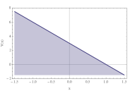
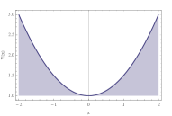
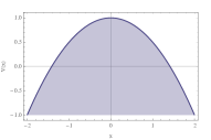
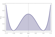
Figure 1: These figures show the potential $V(x)$ for the linear, harmonic oscillator, inverted harmonic oscillator, and double well models. In this paper, we consider the Lorentzian path integral for these potentials.

It should be emphasized that the definition of the Lorentzian path integral (3) is not necessarily the same as the original path integral (I). But, there is a correspondence between these formulations from the definition of path integral,

$$\langle x_{f}\mid e^{-iH(t_{f}-t_{i})}\mid x_{i}\rangle=\int\mathcal{D}x(t)\,e^{{iS[x]}/{\hbar}},$$ (7)

as the Euclidean path integral formulation which is given by the standard Wick rotation $t\rightarrow-i\tau$. The Lorentzian path integral (3) is given by the transformation of $t\rightarrow Nt$ and can be regarded as a complex-time formulation of the path integral by assuming $N$ to be complex.

Although there have been several works on such complex path integral methods Mclaughlin (1972); Aoyama and Harano (1995), there is no obvious choice of integration contours in the complex-time path integral. But, as will be shown later, we solve this problem by using the method of steepest descents or saddle-point method Halliwell and Louko (1989a, b, 1990); Brown and Martinez (1990). Moreover, the Picard-Lefschetz theory allows us to develop this argument more mathematically and rigorously. This theory provides a unique way to find a complex integration contour based on the steepest descent path (Lefschetz thimbles $\cal J_{\sigma}$) and proceed with such oscillatory integral as Witten (2011),

$$\int_{\mathcal{R}}\mathrm{d}x\,\exp\left(\frac{iS[x]}{\hbar}\right)=\sum_{\sigma}n_{\sigma}\int_{\cal J_{\sigma}}\mathrm{d}x\exp\left(\frac{iS[x_{\sigma}]}{\hbar}\right).$$ (8)

where $n_{\sigma}$ is the intersection number of the Lefschetz thimbles $\cal J_{\sigma}$ and steepest ascent path $\cal K_{\sigma}$. In this section, we apply this Lorentzian Picard-Lefschetz method to the tunneling transition of QM.

II.1 Quantum tunneling with Lorentzian path integral

Now, we will consider the linear potential $V=V_{0}-\Lambda x$ with $\Lambda>0$ which corresponds to the no-boundary proposal of the Lorentzian path integral for QG Feldbrugge, Lehners, and Turok (2017a). Thus, we have the following action,

$$S[x,N]=\int_{0}^{1}dtN\left(\frac{\dot{x}^{2}}{2N^{2}}-V_{0}+\Lambda x+E\right),$$ (9)

whose classical solution is given as

$$x_{s}=\frac{\Lambda}{2}N^{2}t^{2}+\left(-\frac{1}{2}N^{2}\Lambda+x_{1}-x_{0}\right)t+x_{0}.$$ (10)

Following Feldbrugge, Lehners, and Turok (2017a); Halliwell and Louko (1989a), we can evaluate the Lorentzian path integral (3) under the semi-classical approximation. We assume the full solution $x(t)=x_{s}(t)+Q(t)$ where $Q(t)$ is the Gaussian fluctuation around the semi-classical solution (10). By substituting it for the action (9) and integrating the path integral over $Q(t)$, we have the following oscillatory integral,

$$K(x_{1};x_{0})=\sqrt{\frac{1}{2\pi i\hbar}}\int_{\mathcal{C}}\frac{\mathrm{d}N}{N^{1/2}}\exp\left(\frac{iS_{0}[N]}{\hbar}\right),$$ (11)

where

$$S_{0}[N]=\int_{0}^{1}dtN\left(\frac{\dot{x}_{s}^{2}}{2N^{2}}-V_{0}+\Lambda x_{s}+E\right)$$

$$=-\frac{\Lambda^{2}N^{3}}{24}-N\left(-\frac{\Lambda}{2}(x_{1}+x_{0})-E+V_{0}\right)+\frac{(x_{1}-x_{0})^{2}}{2N}\,.$$ (12)

Thus, we can calculate the transition amplitude by only performing the integration of the lapse function. Although it is generally difficult to handle such oscillatory integrals, the Picard-Lefschetz theory deals with such integrals. The Picard-Lefschetz theory complexifies the variables and selects a complex path such that the original integral does not change formally via an extension of Cauchy’s integral theorem, and especially pass the saddle points known as the Lefschetz thimbles $\cal J_{\sigma}$.

Now let us integrate the lapse $N$ integral along the Lefschetz thimbles ${\cal J}_{\sigma}$, and we obtain

$$K(x_{1};x_{0}) =\sum_{\sigma}n_{\sigma}\sqrt{\frac{1}{2\pi i\hbar}}\int_{{\cal J}_{\sigma}}\frac{\mathrm{d}N}{N^{1/2}}\exp\left(\frac{iS_{0}[N]}{\hbar}\right).$$ (13)

Since the lapse integral (13) can be approximately estimated based on the saddle points $N_{s}$ and solving ${\partial S_{0}[N]}/{\partial N}=0$, the saddle-points of the action $S_{0}[N]$ are given by,

$$N_{s}=a_{1}\frac{\sqrt{2}}{\Lambda}\left[(\Lambda x_{0}+E-V_{0})^{1/2}+a_{2}(\Lambda x_{1}+E-V_{0})^{1/2}\right],$$ (14)

where $a_{1},a_{2}\in\{-1,1\}$. The four saddle points (14) correspond to the intersection of the steepest descent path $\cal J_{\sigma}$ (Lefschetz thimbles) and steepest ascent path $\cal K_{\sigma}$ where $\textrm{Re}\left[iS_{0}\left(N\right)\right]$ decreases and increases monotonically on $\cal J_{\sigma}$ and $\cal K_{\sigma}$. The saddle-point action $S_{0}[N_{s}]$ evaluated at $N_{s}$ is given by

$$S_{0}[N_{s}]=a_{1}\frac{2\sqrt{2}}{3\Lambda}\left[\left(\Lambda x_{0}+E-V_{0}\right)^{3/2}+a_{2}\left(\Lambda x_{1}+E-V_{0}\right)^{3/2}\right]\,.$$ (15)

Thus, using the saddle-point approximation we can get the following result,

$$K(x_{1};x_{0}) \approx\sum_{\sigma}n_{\sigma}e^{i\theta_{\sigma}}\sqrt{\frac{1}{2\pi i\hbar}}\frac{\exp\left({iS_{0}[N_{s}]/\hbar}\right)}{N_{s}^{1/2}}$$

$$\times\int_{{\cal J}_{\sigma}}\mathrm{d}R\exp\left({-\frac{1}{2\hbar}\left|\frac{\partial^{2}S_{0}[N_{s}]}{\partial N^{2}}\right|R^{2}}\right)$$ (16)

$$\approx\sum_{\sigma}n_{\sigma}e^{i\theta_{\sigma}}\sqrt{\frac{1}{iN_{s}\left|\frac{\partial^{2}S_{0}[N_{s}]}{\partial N^{2}}\right|}}\exp\left(\frac{iS_{0}[N_{s}]}{\hbar}\right)\,,$$

where we expand $S_{0}[N]$ around a saddle point $N_{s}$ as follows,

$$\frac{iS_{0}[N]}{\hbar} =\frac{iS_{0}[N]}{\hbar}\Bigr{|}_{N=N_{s}}-\frac{1}{2\hbar}\left|\frac{\partial^{2}S_{0}[N_{s}]}{\partial N^{2}}\right|R^{2}$$

$$+\frac{i}{6\hbar}\frac{\partial^{3}S_{0}[N]}{\partial N^{3}}\Bigr{|}_{N=N_{s}}(N-N_{s})^{3}+\dots$$ (17)

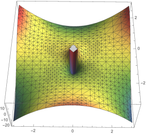
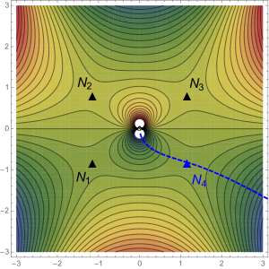
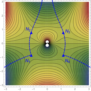
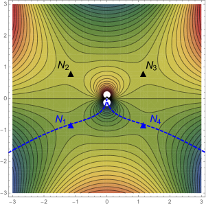
Figure 2: These four figures show $\textrm{Re}\left[iS_{0}\left(N\right)\right]$ in the complex plane where we set $V_{0}=3$, $\Lambda=3$ and $x_{1}=3$. The $x$-axis in these figures corresponds to the real axis of the complex lapse $N$ and the $y$-axis to its imaginary axis. The blue dashed line shows the corresponding the Lefschetz thimbles with the saddle-points; $N_{1}=-\sqrt{\frac{2}{3}}\left(i+\sqrt{2}\right)$, $N_{2}=\sqrt{\frac{2}{3}}\left(i-\sqrt{2}\right)$, $N_{3}=\sqrt{\frac{2}{3}}\left(i+\sqrt{2}\right)$, $N_{4}=-\sqrt{\frac{2}{3}}\left(i-\sqrt{2}\right)$. The upper right figure consider $N=(0,\infty)$ and a Lefschetz thimble with $N_{4}$ can be only chosen. The lower figures take $N=(-\infty,\infty)$ and we can chose two different contours where one pass all saddle points $N_{1,2,3,4}$ and another pass lower two saddle-points $N_{1,4}$. We note that $N_{2,4}$ corresponds to the exponent of the WKB wave function and this point will be discussed in Section III.

From here we will demonstrate the Lorentzian Picard-Lefschetz formulation (13) for QM. Let us consider a simple case with $x_{0}=0$, $E=0$ and $x_{1}>{V_{0}}/{\Lambda}$. Only one Lefschetz thimble can be chosen in the integration domain $\mathcal{R}=(0,\infty)$. Fig. 2 discribes $\textrm{Re}\left[iS_{0}\left(N\right)\right]$ in the complex plane where we set $V_{0}=3$, $\Lambda=3$ and $x_{1}=3$, where the upper right figure suggests that a Lefschetz thimble thorough $N_{4}=-\sqrt{\frac{2}{3}}\left(i-\sqrt{2}\right)$ can be only chosen in $\mathcal{R}=(0,\infty)$. Thus, if we consider the positive lapse $N=(0,\infty)$, we obtain the following result,

$$K(x_{1}) \approx\frac{e^{i\frac{\pi}{4}}}{2^{1/2}V_{0}^{1/4}(\Lambda x_{1}-V_{0})^{1/4}}$$ (18)

$$\times\exp\left({-\frac{2\sqrt{2}i}{3\Lambda\hbar}\left[\left(-V_{0}\right)^{3/2}-\left(\Lambda x_{1}-V_{0}\right)^{3/2}\right]}\right)\,.$$

For the purposes of the later discussion in Section III we consider the case with $V_{0}={\Lambda^{2}}/{2}$ and $x_{1}={V_{0}}/{\Lambda}={\Lambda}/{2}$ and the transition amplitude is written as

$$K(x_{1}) \approx\exp\left({-\frac{\Lambda^{2}}{3\hbar}}\right).$$ (19)

which corresponds to the Euclidean path integral in Section III.

On the other hand, by integrating the complex lapse integral along $\mathcal{R}=(-\infty,\infty)$ and through the four saddle points, we obtain

$$\begin{split}K(x_{1})&\approx C_{1}\,e^{\left({-\frac{2\sqrt{2}i}{3\Lambda\hbar}\left[\left(-V_{0}\right)^{3/2}+\left(\Lambda x_{1}-V_{0}\right)^{3/2}\right]}\right)}\\ &+C_{2}\,e^{\left({\frac{2\sqrt{2}i}{3\Lambda\hbar}\left[\left(-V_{0}\right)^{3/2}-\left(\Lambda x_{1}-V_{0}\right)^{3/2}\right]}\right)}\\ &+C_{3}\,e^{\left({\frac{2\sqrt{2}i}{3\Lambda\hbar}\left[\left(-V_{0}\right)^{3/2}+\left(\Lambda x_{1}-V_{0}\right)^{3/2}\right]}\right)}\\ &+C_{4}\,e^{\left({-\frac{2\sqrt{2}i}{3\Lambda\hbar}\left[\left(-V_{0}\right)^{3/2}-\left(\Lambda x_{1}-V_{0}\right)^{3/2}\right]}\right)},\end{split}$$ (20)

where $C$ is the prefactor at these saddle points, and this Lorentzian amplitude corresponds to the result of Diaz Dorronsoro et al. Diaz Dorronsoro et al. (2017). Strangely, therefore, all the saddle points contribute to the Lorentzian transition amplitude. Fortheremore, as pointed out in Ref Feldbrugge, Lehners, and Turok (2018a) choosing a different contour in $\mathcal{R}=(-\infty,\infty)$ leads to the different transition amplitude,

$$\begin{split}K(x_{1})\approx&\ C_{1}\,e^{\left({-\frac{2\sqrt{2}i}{3\Lambda\hbar}\left[\left(-V_{0}\right)^{3/2}+\left(\Lambda x_{1}-V_{0}\right)^{3/2}\right]}\right)}\\ &+C_{4}\,e^{\left({-\frac{2\sqrt{2}i}{3\Lambda\hbar}\left[\left(-V_{0}\right)^{3/2}-\left(\Lambda x_{1}-V_{0}\right)^{3/2}\right]}\right)}.\end{split}$$ (21)

In Fig. 2 the lower figures consider $N=(-\infty,\infty)$ and we can chose two different contours where one pass all saddle points $N_{1,2,3,4}$ and another pass lower two saddle-points $N_{1,4}$.

Let us consider the Lorentzian path integral (3) and take a different semi-classical approximation to the action (4). In the previous discussion, the action was semi-classically approximated by the solution of the equation of motion (6), but now let us consider the semi-classical approximation of the action (4) by the constraint equation (5). Thus, by solving the constraint equation (5) for $\dot{x}$ and substituting in the action (4), we get the following semi-classical action,

$$S_{0} =\int_{0}^{1}dt[2N(E-V)]=\int_{x_{0}}^{x_{1}}\frac{dx}{\dot{x}}2N(E-V)$$

$$=\pm\int_{x_{0}}^{x_{1}}dx\sqrt{2(E-V)},$$ (22)

where it is important to note that this semi-classical action is different from $S_{0}[N]$ (II.1), cancels and does not have the contribution of $N$ de Alwis (2019).

Furthermore, importantly, the saddle-point of the semi-classical action $S_{0}[N]$ (II.1) is consistent with $S_{0}$ (II.1). In fact, in the linear potential, the sem-classical action is given by

$$S_{0} =\pm\int_{x_{0}}^{x_{1}}dx\sqrt{2(E-V)}=\pm\int_{x_{0}}^{x_{1}}dx\sqrt{2(E-V_{0}+\Lambda x)}$$

$$=\pm\frac{2\sqrt{2}}{3\Lambda}\left[\left(\Lambda x_{0}+E-V_{0}\right)^{3/2}-\left(\Lambda x_{1}+E-V_{0}\right)^{3/2}\right],$$ (23)

which corresponds to the saddle-point action $S_{0}[N_{s}]$ (15). In Section III we will discuss these coincidences in detail. We note that the two saddle points (14) corresponds to the WKB approximation, but other two saddle-points are conjugate for these saddle points.

II.2 Harmonic oscillator and inverted harmonic oscillator models

In the previous subsection, we applied the Lorentzian path integral formulation to the linear potential and discuss some problems with the ambiguity of the lapse function. Let us put these issues aside and consider this Lorentzian formulation to the harmonic oscillator and inverted harmonic oscillator models, which are well known in QM.

First, let us consider the harmonic oscillator model with $V=V_{0}+\frac{1}{2}\Omega^{2}x^{2}$. For simplicity, we consider the zero-energy system with $E=0$ and the solution of the equations of motion is given by

$$x_{s} =x_{0}\cos\left(\Omega Nt\right)-x_{0}\cot\left(\Omega N\right)\sin\left(\Omega Nt\right)$$

$$+x_{1}\csc\left(\Omega N\right)\sin\left(\Omega Nt\right),$$ (24)

where we set $x(0)=x_{0}$ and $x(1)=x_{1}$. By applying the semi-classical approximation to the Lorentzian path integral (3) as well as the linear potential case, we obtain the following integral,

$$K(x_{1};x_{0})=\sqrt{\frac{1}{2\pi i\hbar}}\int_{\mathcal{C}}\frac{\mathrm{d}N}{N^{1/2}}\exp\left(\frac{iS_{0}[N]}{\hbar}\right),$$ (25)

where

$$\begin{split}&S_{0}[N]=\int_{0}^{1}dtN\left(\frac{\dot{x}_{s}^{2}}{2N^{2}}-V_{0}-\frac{1}{2}\Omega^{2}x_{s}^{2}\right)\\ ={}&-NV_{0}+\frac{1}{2}\left(x_{0}^{2}+x_{1}^{2}\right)\Omega\cot\left(\Omega N\right)-x_{0}x_{1}\Omega\csc\left(\Omega N\right)\,.\end{split}$$ (26)

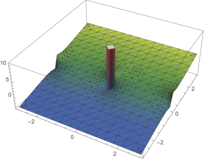
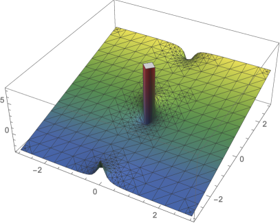
Figure 3: The top and bottom figures show 3D-plot of $\textrm{Re}\left[iS_{0}^{\,\rm saddle}\left(N\right)\right]$ where we take $V_{0}=1$ and $x_{1}=1$ for harmonic and inverted harmonic oscillator models, respectively. The Lefschetz thimbles ${\cal J}_{\sigma}$ on the lapse integral is taken along the imaginary $y$-axis in the harmonic oscillator whereas it is taken along the real $x$-axis for the inverse harmonic oscillator.

When we take $x_{0}=0$ and $\Omega=1$, the semi-classical action $S_{0}[N]$ reads,

$$S_{0}[N]=-NV_{0}+\frac{1}{2}x_{1}^{2}\cot\left(N\right)\,.$$ (27)

By solving ${\partial S_{0}[N]}/{\partial N}=0$, the saddle-points are given as,

$$\sin^{2}\left({N_{s}}\right)=-\frac{x_{1}^{2}}{2V_{0}}\ \Longleftrightarrow\$$ (28)

$$N_{s}=\pm i\sinh^{-1}\sqrt{\frac{x_{1}^{2}}{2V_{0}}}+2\pi c_{1},\ \pi\pm i\sinh^{-1}\sqrt{\frac{x_{1}^{2}}{2V_{0}}}+2\pi c_{1}\,,$$

where $c_{1}\in\mathbb{Z}$. In Fig. 3 we show the contour plot of $\textrm{Re}\left[iS_{0}^{\,\rm saddle}\left(N\right)\right]$ in the complex plane where we set $V_{0}=1$ and $x_{1}=1$ for the harmonic and inverted harmonic oscillator models. Although there are many saddle points, we will simply consider the contour corresponding to $c_{1}=0$ in the integration domain $\mathcal{R}=(0,\infty)$.

Thus, we take one saddle-point $N_{s}=-i\sinh^{-1}\sqrt{\frac{x_{1}^{2}}{2V_{0}}}$ and the saddle-point action is evaluated as

$$S_{0}[N_{s}] =-N_{s}V_{0}+\frac{1}{2}x_{1}^{2}\cot\left(N_{s}\right)$$

$$=iV_{0}\,\sinh^{-1}\sqrt{\frac{x_{1}^{2}}{2V_{0}}}+\frac{ix_{1}\sqrt{V_{0}}}{2}\sqrt{2+\frac{x_{1}^{2}}{V_{0}}}\,,$$ (29)

and we obtain the following transition amplitude,

$$K(x_{1}) \approx\exp\left[\frac{-1}{\hbar}\left(V_{0}\,\sinh^{-1}\sqrt{\frac{x_{1}^{2}}{2V_{0}}}+\frac{x_{1}\sqrt{V_{0}}}{2}\sqrt{2+\frac{x_{1}^{2}}{V_{0}}}\right)\right].$$ (30)

For the purposes of the later discussion in Section III let us consider the specific case which satisfy

$$x_{1}=\frac{\left(e^{2}-1\right)\sqrt{V_{0}}}{\sqrt{2}e},$$ (31)

and the transition amplitude reads

$$K(x_{1}) \approx\exp\left[\frac{\left(1-4e^{2}-e^{4}\right)V_{0}}{4\hbar\,e^{2}}\right].$$ (32)

Next, let us consider the inverted harmonic oscillator model with $V=V_{0}-\frac{1}{2}\Omega^{2}x^{2}$. For simplicity, we consider the zero-energy system with $E=0$ and the solution of the system is given by

$$x_{s}=\frac{e^{-\Omega Nt}\left(-x_{0}e^{2\Omega Nt}+x_{1}e^{2\Omega Nt+\Omega N}+x_{0}e^{2\Omega N}-x_{1}e^{\Omega N}\right)}{e^{2\Omega N}-1}.$$ (33)

By taking semi-classical approximation to the Lorentzian path integral (3) we get the following semi-classical action,

$$\begin{split}&S_{0}[N]=\int_{0}^{1}dtN\left(\frac{\dot{x}_{s}^{2}}{2N^{2}}-V_{0}-\frac{1}{2}\Omega^{2}x_{s}^{2}\right)\\ =&-NV_{0}+\frac{1}{2}\Omega\left(x_{0}^{2}+x_{1}^{2}\right)\coth(N\Omega)-x_{0}x_{1}\Omega\,\text{csch}(N\Omega)\,.\end{split}$$ (34)

We set $x_{0}=0$ and $\Omega=1$, and $S_{0}[N]$ reads,

$$S_{0}[N]=-NV_{0}+\frac{1}{2}x_{1}^{2}\coth\left(N\right)\,.$$ (35)

By solving ${\partial S_{0}[N]}/{\partial N}=0$, the corresponding saddle-points are given by,

$$\begin{split}&\sinh^{2}\left({N_{s}}\right)=-\frac{x_{1}^{2}}{2V_{0}}\ \Longleftrightarrow\ \\ N_{s}=\pm i\sin^{-1}&\sqrt{\frac{x_{1}^{2}}{2V_{0}}}+2i\pi c_{2},\ i\pi\pm i\sin^{-1}\sqrt{\frac{x_{1}^{2}}{2V_{0}}}+2i\pi c_{2}\,,\end{split}$$ (36)

where $c_{2}\in\mathbb{Z}$. As before, we consider the contour corresponding to $c_{2}=0$ in $\mathcal{R}=(0,\infty)$. Hence, we take $N_{s}=-i\sin^{-1}\sqrt{\frac{x_{1}^{2}}{2V_{0}}}$ and the saddle-point action $S_{0}[N_{s}]$ is evaluated as

$$S_{0}[N_{s}] =-N_{s}V_{0}+\frac{1}{2}x_{1}^{2}\coth\left(N_{s}\right)$$

$$=iV_{0}\,\sin^{-1}\sqrt{\frac{x_{1}^{2}}{2V_{0}}}+\frac{ix_{1}\sqrt{V_{0}}}{2}\sqrt{2-\frac{x_{1}^{2}}{V_{0}}}\,.$$ (37)

For the later discussion in Section III, let us consider the following case,

$$x_{1}=\sqrt{2V_{0}}\sin(1),$$ (38)

and the transition amplitude reads

$$K(x_{1}) \approx\exp\left(-\frac{V_{0}+V_{0}\sin(1)\cos(1)}{\hbar}\right).$$ (39)

III Euclidean path integral, instanton and WKB approximation

In this section, we review the Euclidean path integral, instanton and WKB approximation for the quantum tunneling and discuss their relations to the Lorentzian Picard-Lefschetz formulation (13).

III.1 Euclidean path integral and instanton

The evolution of the wave function in the classical regime can be approximated by saddle points $\delta S[x]/\delta x\approx 0$ which satisfy the classical equation of motion. On the other hand, for quantum tunneling path which is the classically forbidden region the transition amplitude is approximately given by the saddle points of the Euclidean path integral which is derived by the solution of the Euclidean equations of motion.

We can easily show that setting $N=-i$ the Lorentzian path integral (3) corresponds to the Euclidean amplitude. In fact, the reparameterized action $S[x,N]$ is given by $t\rightarrow Nt$ in $S[x]$ and the Euclidean action $S_{E}[x]$ is given by $t\rightarrow-i\tau$. Therefore, the action $S[x,-i]$ represents the Euclidean action $S_{E}[x]$,

$$iS[x,-i]=-\int_{t_{i}}^{t_{f}}dt\left(\frac{\dot{x}^{2}}{2}+V(x)\right)$$ (40)

$$\iff iS[x]\equiv-S_{E}[x]=-\int_{\tau_{i}}^{\tau_{f}}\mathrm{d}\tau\left(\frac{1}{2}\left(\frac{dx}{d\tau}\right)^{2}+V(x)\right)\,,$$

where the potential changes sign $V(x)\rightarrow-V(x)$ in $S_{E}[x]$. From (73) we derive the following Euclidean equations of motion,

$$\frac{d^{2}x}{d\tau^{2}}=V^{\prime}(x).$$ (41)

However, the extrema of $N$ corresponding to the saddle points of the Lorentzian path integral (3) using the Picard-Lefschetz theory deviate from $N=-i$ and do not reproduce the transition amplitude based on the Euclidean path integral. From here we show some examples to clarify this fact. Let us consider the linear potential $V=V_{0}-\Lambda x$ with $\Lambda>0$ for simplicity. Note that solving the Euclidean equations of motion and substituting the solutions for the Euclidean action $S_{E}[x]$ leads to the instanton amplitude. Therefore, the oscillatory integral (11) is consistent with the Euclidean amplitude except for the lapse integral. Thus, by taking $N=-i$ we have the Euclidean transition amplitude for the linear potential,

$$K(x_{1};x_{0})=\sqrt{\frac{-1}{2\pi\hbar}}e^{iS_{0}[-i]/\hbar}=\sqrt{\frac{-1}{2\pi\hbar}}e^{-S_{E}/\hbar},$$ (42)

where $S_{E}$ is

$$\begin{split}S_{E}&=\int_{\tau_{i}=0}^{\tau_{f}=1}\mathrm{d}\tau\left\{\frac{1}{2}\left(\frac{dx_{s}}{d\tau}\right)^{2}+V_{0}-\Lambda x_{s}\right\}\\ &=-\frac{\Lambda^{2}}{24}-\frac{\Lambda}{2}(x_{1}+x_{0})+V_{0}+\frac{(x_{1}-x_{0})^{2}}{2}\,.\end{split}$$ (43)

For simplicity, we consider $x_{0}=0$ and the transition amplitude is given by

$$K(x_{1}) \approx\exp\left[{-\frac{1}{\hbar}\left(-\frac{\Lambda^{2}}{24}-\frac{\Lambda x_{1}}{2}+V_{0}+\frac{x_{1}^{2}}{2}\right)}\right],$$ (44)

which is not consistent with the result (18) of the Lorentizan path integral. As we will see later, this result is not compatible with the WKB approximation either.

The reason is that the semi-classical solution (10) with $N=-i$ does not satisfy the constraint equation (5), which is the law of conservation of energy. Thus, when the constraint equation (5) is actually satisfied the result of the Euclidean path integral coincides with the Lorentzian Picard-Lefschetz formulation (18). For instance, when we take $V_{0}={\Lambda^{2}}/{2}$ and $x_{1}={V_{0}}/{\Lambda}={\Lambda}/{2}$ and the transition amplitude is given by

$$K(x_{1}) \approx\exp\left({-\frac{\Lambda^{2}}{3\hbar}}\right),$$ (45)

which is consistent with the result (19) in the Lorentzian Picard-Lefschetz formulation. In this case the saddle points of the action (15), which is $N_{s}=\pm i$ also coincides with the Euclidean saddle point $N=-i$. In Fig. 4 we show this correspondence.

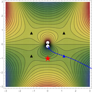
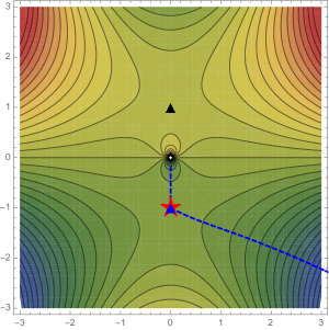
Figure 4: The top figure shows $\textrm{Re}\left[iS_{0}^{\,\rm saddle}\left(N\right)\right]$ in complex plane where we set $V_{0}=3$, $\Lambda=3$ and $x_{1}=3$ and the star expresses $N=-i$. On the other hand, in the bottom figure we set $V_{0}=9/2$, $\Lambda=3$ and $x_{1}=3/2$ and this figure shows that the saddle points of the action (15) is $N_{s}$ also coincides with the Euclidean saddle point $N=-i$.

Next, let us discuss the well-known double well potential,

$$V(x)=\frac{\lambda}{4}\left(x^{2}-a^{2}\right)^{2},$$ (46)

and consider the quantum tunneling from $x_{0}=-a$ to $x_{1}=a$. The usual method for finding the Euclidean (instanton) solution in this case, is to obtain it directly from the Euclidean energy conservation rather than solving the Euclidean equations of motion. For simplicity, we set $E=0$ and the Euclidean energy conservation gives,

$$\frac{1}{2}\left(\frac{dx}{d\tau}\right)^{2}-V(x)=0\ \Longrightarrow\ \frac{dx}{d\tau}=\pm\sqrt{\frac{\lambda}{2}}\left(x^{2}-a^{2}\right).$$ (47)

Thus, we can get the following instanton solution interpolating between $-a$ and $a$,

$$x(\tau)=\pm\,a\tanh\frac{\omega}{2}\left(\tau-\tau_{0}\right),$$ (48)

where $\omega=\sqrt{2\lambda a^{3}}$ and $\tau_{0}$ is an integration constant. The plus and minus classical solutions are the instanton and anti-instanton. The instanton corresponds to the particle initially sitting on the maximum of $-V(x)$ at $x=-a$, passing $x=0$ for a very short time and ending up at the other maximum of $-V(x)$ at $x=a$. From the instanton the Euclidean action is given by

$$S_{E}=\frac{2\sqrt{2\lambda}\,a^{3}}{3},$$ (49)

whose the transition amplitude $K(a)$ is consistent with the WKB approximation of the wave function. For instance, if we extend this instanton as follows,

$$x(t)=a\tanh\frac{\omega}{2}\left(iNt-\tau_{0}\right),$$ (50)

and apply it to the Lorentzian Picard-Lefschetz formulation, it returns the same result. As already discussed, a saddle-point approximation of the action by a solution of the Euclidean equations of motion does not give the correct transition amplitude. The correct result is obtained when the solution of the Euclidean equation of motion satisfies the energy conservation. Since the instanton solution is derived from the energy conservation in Euclidean form, it necessarily corresponds to the saddle point of the Lorentzian path integral. It is important to note that the solutions of the Euclidean equation of motion do not necessarily correspond to the correct semiclassical saddle point solutions. It is physically meaningful only if the solutions satisfy the constraint equation (5).

We can see the same relations with the harmonic oscillator and inverted harmonic oscillator models. By taking $N=-i$ we have the Euclidean transition amplitude for the harmonic and inverted harmonic oscillator,

$$K^{H}(x_{1};x_{0}) \approx e^{\left[{-\frac{1}{\hbar}\left(V_{0}+\frac{1}{2}\left(x_{0}^{2}+x_{1}^{2}\right)\Omega\coth\Omega-x_{0}x_{1}\Omega\,\text{csch}\,\Omega\right)}\right]},$$ (51)

$$K^{I}(x_{1};x_{0}) \approx e^{\left[{-\frac{1}{\hbar}\left(V_{0}+\frac{1}{2}\left(x_{0}^{2}+x_{1}^{2}\right)\Omega\cot\Omega-x_{0}x_{1}\Omega\,\text{csc}\,\Omega\right)}\right]},$$ (52)

where we denote that $K^{H}(x_{1};x_{0})$, $K^{I}(x_{1};x_{0})$ are the transition amplitudes for the harmonic and inverted harmonic oscillator are not consistent with the Lorentizan formulations (30). As discussed previously, when we take $x_{0}=0$ and $\Omega=1$ and choose $x_{1}$ which satisfies the Euclidean energy conservation,

$$x_{1}^{H}=\frac{\left(e^{2}-1\right)\sqrt{V_{0}}}{\sqrt{2}e},\quad x_{1}^{I}=\sqrt{2V_{0}}\sin(1),$$ (53)

the Euclidean transition amplitudes are consistent with the results (32) and (39) of the Lorentzian formulation,

$$K^{H}(x_{1}) \approx\exp\left(\frac{\left(1-4e^{2}-e^{4}\right)V_{0}}{4\hbar e^{2}}\right),$$ (54)

$$K^{I}(x_{1}) \approx\exp\left(-\frac{V_{0}+V_{0}\sin(1)\cos(1)}{\hbar}\right).$$ (55)

III.2 WKB approximation of Schrödinger equation

Let us discuss the WKB approximation of the Schrödinger equation and the correspondence to the Lorentzian and Euclidean path integral formulation. The WKB approximation (or WKB method) is one of the semi-classical approximation methods for the Schrödinger equation. For the Schrödinger equation, which is the fundamental equation of QM and reads,

$$\hat{H}\Psi(x)=\left(-\frac{\hbar^{2}}{2}\frac{d^{2}}{dx^{2}}+V(x)\right)\Psi(x)=E\,\Psi(x),$$ (56)

where $\hat{H}$ is the Hamiltonian, we assume that the solution is in the form of $\exp\,(\frac{i}{\hbar}S[x])$ and expanded as a perturbation series of $\hbar$. By substituting $\Psi(x)\approx e^{\frac{i}{\hbar}\left(S_{0}[x]+\hbar S_{1}[x]+\cdots\right)}$ in the Schrödinger equation (56) we obtain the following equations,

$$\frac{1}{2}\left(\frac{dS_{0}}{dx}\right)^{2}+V-E=0,\quad\frac{dS_{1}}{dx}=\frac{i}{2}\frac{d}{dx}\left(\ln\frac{dS_{0}}{dx}\right)\dots,$$ (57)

where $S_{0}$ is the dominant contribution of the WKB wave function and can also be obtained by the constraint equation (5) as already discussed in Section II. We note that the Schrödinger equation (56) and wave function do not have the contribution of $N$ even if the semi-classical action includes the lapse function $N$.

In the leading order of the WKB approximation the wave function is given by

$$\Psi(x)\approx\frac{c}{|2(E-V(x))|^{1/4}}e^{\left[{\pm\frac{i}{\hbar}\int^{x}_{x_{0}}dx\sqrt{2(E-V(x))}}\right]}\,.$$ (58)

For the linear potential the WKB wave function is given by

$$\begin{split}&\Psi(x)\approx\ \frac{c_{1}e^{\left({+\frac{2\sqrt{2}i}{3\Lambda\hbar}\left[\left(\Lambda x_{0}+E-V_{0}\right)^{3/2}-\left(\Lambda x_{1}+E-V_{0}\right)^{3/2}\right]}\right)}}{|2(E-V(x))|^{1/4}}\,\\ &+\frac{c_{2}e^{\left({-\frac{2\sqrt{2}i}{3\Lambda\hbar}\left[\left(\Lambda x_{0}+E-V_{0}\right)^{3/2}-\left(\Lambda x_{1}+E-V_{0}\right)^{3/2}\right]}\right)}}{|2(E-V(x))|^{1/4}}\,,\end{split}$$ (59)

where the exponent of the above WKB wave function agrees with the two saddle-point actions $S_{0}[N_{s}]$ (15) of the Lorentzian path integral. In the Lorentzian Picard-Lefschetz formulation (13), four-saddle points dominate the path integral, and only one saddle point contributes when the lapse integral is defined as positive. On the other hand, in the WKB analysis, there is no uncertainty of the lapse function, and the exponents of the wave function can be either positive or negative, depending on the initial conditions. Thus, the positive and negative lapse function in the Lorentzian Picard-Lefschetz formulation (13) could be considered.

On the other hand, for the harmonic and inverted harmonic oscillator potentials where we take $x_{0}=0$ and $E=0$, the exponents of the WKB wave function are given by

$$S_{0} =\pm iV_{0}\,\sinh^{-1}\sqrt{\frac{x_{1}^{2}}{2V_{0}}}\pm\frac{ix_{1}\sqrt{V_{0}}}{2}\sqrt{2+\frac{x_{1}^{2}}{V_{0}}}\,,$$ (60)

$$S_{0} =\pm iV_{0}\,\sin^{-1}\sqrt{\frac{x_{1}^{2}}{2V_{0}}}\pm\frac{ix_{1}\sqrt{V_{0}}}{2}\sqrt{2-\frac{x_{1}^{2}}{V_{0}}}\,,$$ (61)

which are exactly consistent with the saddle points of the Lorentzian formulation (II.2) and (II.2). Finally, we comment the double well potential (4) with zero-energy system $E=0$ and the corresponding semi-classical action is given by

$$S_{0} =\pm\int_{x_{0}=-a}^{x_{1}=a}dx\sqrt{-\frac{\lambda}{2}\left(x^{2}-a^{2}\right)^{2}}=\pm i\frac{2\sqrt{2\lambda}\,a^{3}}{3},$$ (62)

which is consistent with the Euclidean action $S_{E}$ utilizing the instanton (49). In summary the Lorentzian Picard-Lefschetz formulation (13) including the lapse $N$ integral and using the Picard-Lefschetz theory, and the Euclidean formulation utilizing instanton are nothing more than the WKB analysis of the Schrödinger equation.

The reason why these approaches correspond is as follows: Applying the method of steepest descents or saddle-point using the Picard-Lefschetz theory to the integration of the lapse $N$ corresponds to taking semi-classical contours such that the constraint equation (5) is satisfied. Therefore, the Lorentzian Picard-Lefschetz formulation (13) corresponds to the WKB approximation to the wave function whose $S_{0}$ is given by the constraint equation (5). Conversely, in order for the Euclidean path integral $S_{E}$ to be the correct semiclassical approximation, the solutions of the Euclidean equation of motion must satisfy the constraint equation (5).

IV Lorentzian Picard-Lefschetz Formulation for quantum gravity

In this section we demonstrate that the tunneling or no-boundary wave functions derived by the Lorentzian Picard-Lefschetz Formulation corresponds to the WKB solution of the Wheeler-DeWitt equation Brown and Martinez (1990); Vilenkin and Yamada (2018); de Alwis (2019).

Following Halliwell and Louko (1989a) the gravitational amplitude based on Arnowitt, Deser and Misner (ADM) formalism Arnowitt, Deser, and Misner (2008) can be written by the Lorentzian path integral,

$$G(q_{f};q_{i})=\int_{\mathcal{C}}\mathrm{d}N\int\mathcal{D}q(t)~{}\exp\left(\frac{iS[N,q]}{\hbar}\right)~{}.$$ (63)

where $S[N,q]$ is the gravitational action with $q=a^{2}$. Since $S[N,q]$ is quadratic, the functional integral (63) can be evaluated under the semi-classical approximation. We assume $q(t)=q_{s}(t)+Q(t)$ where $Q(t)$ is the Gaussian fluctuation around the semi-classical solution. By substituting it for $S[N,q]$ and integrating the path integral over $Q(t)$, we have the following expression Feldbrugge, Lehners, and Turok (2017a),

$$G(q_{f};q_{i})=\sqrt{\frac{3\pi i}{2\hbar}}\int_{\mathcal{C}}\frac{\mathrm{d}N}{N^{1/2}}\exp\left(\frac{iS_{0}[N]}{\hbar}\right),$$ (64)

where $S_{0}[N]$ is the semi-classical action,

$$S_{0}[N]=2\pi^{2}\int_{0}^{1}\mathrm{d}t\left(-\frac{3}{4N}\dot{q}_{s}^{2}+3KN-N\Lambda q_{s}\right)$$

$$=2\pi^{2}\left\{\frac{N^{3}\Lambda^{2}}{36}+N\left(-\frac{\Lambda(q_{i}+q_{f})}{2}+3K\right)-\frac{3(q_{f}-q_{i})^{2}}{4N}\right\}\,.$$ (65)

We wil integrate the lapse integral along the Lefschetz thimbles ${\cal J}_{\sigma}$ as follows,

$$G(q_{1};q_{0}) =\sum_{\sigma}n_{\sigma}\sqrt{\frac{3\pi i}{2\hbar}}\int_{{\cal J}_{\sigma}}\frac{\mathrm{d}N}{N^{1/2}}\exp\left(\frac{iS_{0}[N]}{\hbar}\right).$$ (66)

The lapse integral (66) can be estimated based on the four saddle points $N_{s}$,

$$N_{s}=a_{1}\frac{3}{\Lambda}\left[\left(\frac{\Lambda}{3}q_{0}-K\right)^{1/2}+a_{2}\left(\frac{\Lambda}{3}q_{1}-K\right)^{1/2}\right],$$ (67)

where $a_{1},a_{2}\in\{-1,1\}$. The four saddle points (67) correspond to the intersection of the Lefschetz thimble $\cal J_{\sigma}$ and steepest ascent paths $\cal K_{\sigma}$ where $\textrm{Re}\left[iS_{0}\left(N\right)\right]$ decreases and increases monotonically on $\cal J_{\sigma}$ and $\cal K_{\sigma}$, and $n_{\sigma}$ is the intersection number. The saddle-point action $S_{0}[N_{s}]$ is given by

$$S_{0}[N_{s}]=-a_{1}\frac{12\pi^{2}}{\Lambda}\left[\left(\frac{\Lambda}{3}q_{0}-K\right)^{3/2}+a_{2}\left(\frac{\Lambda}{3}q_{1}-K\right)^{3/2}\right]\,.$$ (68)

By imposing the condition $q_{0}=0$, $K=1$ Hartle and Hawking (1987), and assuming $q_{1}{\Lambda}>{3}$, the gravitational amplitude (64) corresponds to the cosmological wave function created from nothing $q=0$. Based on the Lorentzian Picard-Lefschetz method, Feldbrugge et al. Feldbrugge, Lehners, and Turok (2017a) showed that the gravitational transition amplitude (64) by perfuming the integral over a contour in $(0,\infty)$ reduces to the Vilenkin’s tunneling wave function Vilenkin (1982). On other hand, Diaz Dorronsoro et al. Diaz Dorronsoro et al. (2017) reconsidered the gravitational amplitude (66) by integrating the lapse over a different contour in $(-\infty,\infty)$ and showed that the gravitational amplitude (66) reduces to be the Hartle-Hawking’s no boundary wave function Hartle and Hawking (1987).

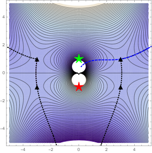
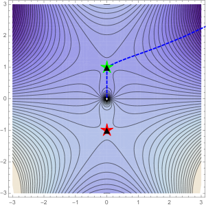
Figure 5: In the top figure we set $q_{1}=10$ and $\Lambda=3$. The blue dashed line shows the Lefschetz thimbles on $N=(0,\infty)$ whereas the black dashed line shows the Lefschetz thimbles on $N=(-\infty,\infty)$. The red or green star express the standard or inverted Wick rotation, $N=+i,-i$. On the other hand, in the bottom figure we take $q_{1}=1$ and $\Lambda=3$ and this figure shows $N_{s}$ coincides with the anti-Euclidean saddle point $N=+i$. Thus, the tunneling wave function based on the Lorentzian Picard-Lefschetz Formulation consistent with the Linde wave function Linde (1984).

The top figure of Fig. 5 discribes $\textrm{Re}\left[iS_{0}\left(N\right)\right]$ in the complex plane where we set $V_{0}=3$, $\Lambda=3$ and $q_{1}=10$. In the top figure of Fig. 5 the Picard-Lefschetz theory says that only one Lefschetz thimble can be chosen in the integration domain $N=(0,\infty)$. On the other hand, integrating the complex lapse integral along $N=(-\infty,\infty)$ all four saddle points can contribute the gravitational amplitude (66) although as pointed out in Ref Feldbrugge, Lehners, and Turok (2018a) one can choose a different contour in $N=(-\infty,\infty)$. Hence, the gravitational amplitude (66) leads to the tunneling and no-boundary wave function,

$$G_{T}(q_{1})\approx c_{1}e^{-\frac{12\pi^{2}}{\hbar\Lambda}\,-i4\pi^{2}\sqrt{\frac{\Lambda}{3}}(q_{1}-3/\Lambda)^{3/2}/\hbar}\,,$$ (69)

$$G_{HH}(q_{1})\approx c_{1}e^{-\frac{12\pi^{2}}{\hbar\Lambda}\,-i4\pi^{2}\sqrt{\frac{\Lambda}{3}}(q_{1}-3/\Lambda)^{3/2}/\hbar}$$

$$+c_{2}e^{-\frac{12\pi^{2}}{\hbar\Lambda}\,+i4\pi^{2}\sqrt{\frac{\Lambda}{3}}(q_{1}-3/\Lambda)^{3/2}/\hbar}$$

$$+c_{3}e^{+\frac{12\pi^{2}}{\hbar\Lambda}\,+i4\pi^{2}\sqrt{\frac{\Lambda}{3}}(q_{1}-3/\Lambda)^{3/2}/\hbar}$$

$$+c_{4}e^{+\frac{12\pi^{2}}{\hbar\Lambda}\,-i4\pi^{2}\sqrt{\frac{\Lambda}{3}}(q_{1}-3/\Lambda)^{3/2}/\hbar}\,,$$ (70)

where $c_{1,2,3}$ include the functional determinants and prefactors.

Let us consider the gravitational amplitude (63) again but take a different semi-classical approximation to the gravitational action. In the previous discussion, the gravitational action was semi-classically approximated by the classical solutions of the equation of motion, but we can approximate the gravitational action by utilizing the constraint equation as discussed in Section III. Thus, by solving the constraint equation for $\dot{q}$ and substituting in the action, we can obtain the semi-classical gravitational action as follows Brown and Martinez (1990); Vilenkin and Yamada (2018); de Alwis (2019),

$$\begin{split}&S_{0}[q_{1};q_{0}]=4\pi^{2}\int_{t_{0}}^{t_{1}}Ndt\left(3K-\Lambda q\right)\\ &=\pm\,2\sqrt{3}\pi^{2}\int_{q_{0}}^{q_{1}}dq\sqrt{\Lambda q-3K}\\ &=\pm\frac{12\pi^{2}}{\Lambda}\left[\left(\frac{\Lambda}{3}q_{0}-K\right)^{3/2}-\left(\frac{\Lambda}{3}q_{1}-K\right)^{3/2}\right],\end{split}$$ (71)

which cancels the lapse $N$ contribution de Alwis (2019) and corresponds to the semi-classical action under the WKB approximation. In fact, in the leading order the WKB wave function is given by

$$\Psi[q_{1};q_{0}]\approx C\cdot\exp\left[{\pm\frac{i\,2\sqrt{3}\pi^{2}}{\hbar}\int_{q_{0}}^{q_{1}}dq\sqrt{\Lambda q-3K}}\right]\,.$$ (72)

where the exponent of the above WKB wave function agrees with the two saddle-point actions (68).

From here, let us discuss the relation between the wave function in the Lorentzian Picard-Lefschetz Formulation and the Hartle-Hawking or Linde wave function given by the Euclidean path integral. We can easily see that setting $N=-i$ the Lorentzian path integral corresponds to the Euclidean path integral since $S[q,N]$ is given by the Wick-rotation $t\rightarrow Nt$ and $S_{E}[q]$ is given by $t\rightarrow-i\tau$. For simplicity, considering the original gravitational action $S[a]$ and redefining the time $t=\tau$, the Euclidean action $S_{E}[a]$ for the closed universe with $K=1$ is given by

$$\begin{split}&iS[a,-i]\equiv-S_{E}[a]\\ &=2\pi^{2}\int_{0}^{\tau}\mathrm{d}\tau\left(3a\left(\frac{da}{d\tau}\right)^{2}+3a-3a^{3}H^{2}\right),\end{split}$$ (73)

where $H^{2}=\Lambda/3$ and $S_{E}[a]$ is negative for small $a$. From (73) we obtain the Euclidean constraint equation and the equations of motion,

$$\left(\frac{da}{d\tau}\right)^{2}-1+a^{2}H^{2}=0,\quad\left(\frac{d^{2}a}{d\tau^{2}}\right)=-aH^{2}.$$ (74)

Hence, we obtain the Euclidean de Sitter solution $a(\tau)=H^{-1}\sin H\tau$ with the initial condition $a(0)=0$. Note that in the saddle point method of the Euclidean path integral, the classical solution of the saddle point is not correct unless not only the equations of motion but also the constraint equation are satisfied.

By using the classical saddle-point solution we can evaluate the Euclidean action under the saddle-point approximation,

$$S_{E}[a] =-2\pi^{2}\int_{0}^{\pi/2H}\mathrm{d}\tau\left(3a\left(\frac{da}{d\tau}\right)^{2}+3a-3a^{3}H^{2}\right)$$

$$=-\frac{12\pi^{2}}{\Lambda}\ .$$ (75)

Thus, we have the Hartle-Hawking wave function,

$$\Psi_{HH}(a)\sim\exp\left(-S_{E}[a]\right)\sim\exp\left(+\frac{12\pi^{2}}{\Lambda}\right).$$ (76)

which diverges the probability and disfavors the inflationary cosmology if we replace the cosmological constant $\Lambda$ with the scalar potential $V(\phi)$. On the other hand, to suppress the exponential probability and get the cosmological wave function of the ground state, Linde Linde (1984) proposed the wave function utilizing the anti-Wick rotation $\tau=-it$,

$$\Psi_{L}(a)\sim\exp\left(+S_{E}[a]\right)\sim\exp\left(-\frac{12\pi^{2}}{\Lambda}\right),$$ (77)

Now, we can easily show that the wave function from the Lorentzian Picard-Lefschetz Formulation and WKB method includes the Hartle-Hawking or Linde wave function given by the saddle point method of the Euclidean path integral. As already mentioned, the de Sitter solution $a(\tau)=H^{-1}\sin H\tau$ is a saddle-point solution with zero energy, and the final scale factor is $a(\tau)=H^{-1}$. In other words, the saddle-point method of Euclidean path integral only gives the transition amplitude from the entry to the exit of the potential in the quantum tunneling. In the Lorentzian Picard-Lefschetz Formulation and WKB approximation method, such a transition amplitude can be given by $\Lambda q_{1}-3K=0$. Thus, we get the corresponding transition amplitude,

$$\Psi[q_{1}] \approx\sqrt{\frac{3\pi i}{2\hbar}}\int_{0,-\infty}^{+\infty}\frac{\mathrm{d}N}{N^{1/2}}\exp\left(\frac{iS_{0}[N]}{\hbar}\right)$$

$$\approx\exp\left(\pm\frac{12\pi^{2}}{\Lambda}\right)\,.$$ (78)

where we note that the four saddle points (67) of the semi-classical action $S_{0}[N]$ in the Lorentzian Picard-Lefschetz method converges on the two saddle points $N_{s}=\pm i$. In the bottom figure of Fig. 5 we show the correspondence.

V Quantum tunneling with Lorentzian instanton

In this section, we will introduce a new instanton method based on the previous discussions. As discussed in Section III, the Euclidean saddle-point action corresponding to the exponent of the WKB wave function does not consist only of the simple solutions of the equation of motion. The solutions of the Euclidean equation of motion must satisfy the constraint equation (5) in the Euclidean form. The Lorentzian Picard-Lefschetz formulation Feldbrugge, Lehners, and Turok (2017a) constructs the semi-classical transition amplitude by finding saddle points on the lapse integration which implies $\delta S[x,N]/\delta N=0$. Since $\delta S[x,N]/\delta N=0$ corresponds to the constraint equation (5), the transition amplitude becomes consistent with the WKB approximation for wave-function. Hence, we can expect to obtain the saddle-point action corresponding to the WKB approximation by finding the Lorentzian solution from the constraint equation (5) and substituting it into the Lorentzian action. We will now briefly introduce the method and call it $\it Lorentzian\ instanton\ formulation$.

Let us write the Lorentzian path integral including lapse function $N_{L}$ again,

$$K(x_{f};x_{i}) =\int_{x_{i}}^{x_{f}}\mathcal{D}x~{}\exp\left(\frac{iS[x]}{\hbar}\right),$$ (79)

$$S[x] =\int_{t_{i}}^{t_{f}}dtN_{L}\left(\frac{\dot{x}^{2}}{2N_{L}^{2}}-V(x)+E\right),$$ (80)

which fixes the lapse $N_{L}$ and does not integrate. From (79) we derive the constraint equation and the equations of motion,

$$\delta S[x]/\delta{N_{L}} =0\ \Longrightarrow\ \frac{\dot{x}^{2}}{2}+N_{L}^{2}V(x)=N_{L}^{2}E,$$ (81)

$$\delta S[x]/\delta{x} =0\ \Longrightarrow\ \ddot{x}=-N_{L}^{2}V^{\prime}(x).$$ (82)

As is well known in analytical mechanics, the equation of motion (81) is obtained by differentiating the constraint equation (82). Thus, only the constraint equation is considered. Solving the constraint equation (82) for $x$ with the initial condition $x(t_{i})=x_{0}$, we get one semi-classical solution. Then, we impose the final condition $x(t_{f})=x_{1}$ on the solution and determine the lapse function $N_{L}$ on the complex path. Thus, we can get the Lorentzian real-time solution even for quantum tunneling and construct the path integral (79) from the Lorentzian classical solution as well as the instanton method based on the Euclidean path integral.

From here, we will show that this formulation is consistent with Lorentzian Picard-Lefschetz formulation (13) and WKB approximation for the wave function. For simplicity, let us consider the linear potential $V=V_{0}-\Lambda x$ and assume $t_{i}=0$ and $t_{f}=1$. The constraint equation (82) with the initial condition $x(t_{i}=0)=x_{0}$ gives the following classical solution,

$$x_{L}(t)=x_{0}+\frac{\Lambda}{2}N_{L}^{2}t^{2}\pm N_{L}t\sqrt{2E-2V_{0}+2\Lambda x_{0}}.$$ (83)

By imposing the final condition $x(t_{f}=1)=x_{1}$ on the solution we can determine the lapse function $N_{L}$ and obtain,

$$N_{L}=\mp\frac{\sqrt{2}}{\Lambda}\left[(\Lambda x_{0}+E-V_{0})^{1/2}\pm(\Lambda x_{1}+E-V_{0})^{1/2}\right],$$

$$x_{L}(t)=x_{0}+\left[(\Lambda x_{0}+E-V_{0})^{1/2}\pm(\Lambda x_{1}+E-V_{0})^{1/2}\right]^{2}t^{2}$$

$$-\frac{\sqrt{2}\,t}{\Lambda}\left[(\Lambda x_{0}+E-V_{0})^{1/2}\pm(\Lambda x_{1}+E-V_{0})^{1/2}\right]$$

$$\times\sqrt{2E-2V_{0}+2\Lambda x_{0}}.$$ (84)

where $N_{L}$ corresponds to the four saddle points (14) of the Lorentzian Picard-Lefschetz formulation and $x_{L}(t)$ is given by imposing $N_{L}$ to the Lorentzian solution (83). Note that plus sign solution in Eq. (84) is non-trivial since it is non-zero in the limit $x_{1}\rightarrow x_{0}$. Here, the degree of freedom of lapse is uniquely determined. Thus, the semi-classical action $S[x_{L}]$ is given by

$$S[x_{L}] =\pm\frac{2\sqrt{2}}{3\Lambda}\left[\left(\Lambda x_{0}+E-V_{0}\right)^{3/2}\pm\left(\Lambda x_{1}+E-V_{0}\right)^{3/2}\right].$$ (85)

which is consistent with the semi-classical action for the WKB wave function and saddle-point action (15) of the Lorentzian Picard-Lefschetz formulation. By developing the saddle point method where $x=x_{L}+\delta x$ is decomposed as the Lorentzian classical solutions and the fluctuation around them, the Lorentzian transition amplitude can be approximately given by

$$\begin{split}&K(x_{1};x_{0})\simeq\exp\left(\frac{iS[x_{L}]}{\hbar}\right)\int_{\delta x(0)=0}^{\delta x(1)=0}\mathcal{D}\delta x\,e^{\left(\frac{i}{2\hbar}\frac{\delta^{2}S[x]}{\delta x^{2}}\Bigr{|}_{x=x_{L}}\delta x^{2}\right)}\\ &\simeq\exp\left(\frac{iS[x_{L}]}{\hbar}\right)\int_{\delta x(0)=0}^{\delta x(1)=0}\mathcal{D}\delta x\,e^{\left(\frac{i}{2\hbar N_{L}}\int_{0}^{1}dt\left(\delta\dot{x}^{2}-V^{\prime\prime}(x_{L})\delta x^{2}\right)\right)}\\ &\simeq\sqrt{\frac{1}{2\pi i\hbar N_{L}}}\exp\left(\frac{iS[x_{L}]}{\hbar}\right),\end{split}$$ (86)

where $V^{\prime\prime}(x_{L})$ is zero for the linear potential. Note that this method still has a problem how to select the correct Lorentzian solutions. Let us compare this result with the real-time path integral for the linear potential. Following Feynman’s famous textbook Feynman, Hibbs, and Styer (2010), the real-time transition amplitude is approximately given by

$$\begin{split}K(x_{1};x_{0})&\simeq\sqrt{\frac{1}{2\pi i\hbar}}e^{\left[\frac{i}{\hbar}\left\{\frac{(x_{1}-x_{0})^{2}}{2}+\frac{\Lambda(x_{1}+x_{0})}{2}-\frac{\Lambda^{2}}{24}\right\}\right]},\end{split}$$ (87)

which does not agree with the Lorentzian formulation (86). However, in this saddle point approximation the classical path solution does not respect the constraint equation (6) and if we explicitly write the energy of the system and usually think about that, $x_{1,0}$ is restricted by $E$ as classical mechanics. By imposing the constraint (6) on the real-time classical solution and setting $x_{0}=0$ and $V_{0}=E=0$ for simplicity, the real-time transition amplitude (87) agrees with the Lorentzian amplitude (86),

$$K(x_{1};0)\simeq\sqrt{\frac{1}{2\pi i\hbar}}\exp\left(\frac{4ix_{1}^{2}}{3\hbar}\right).$$ (88)

As discussed in Section III, the Lorentzian transition amplitudes, which approximate the saddle point from the constraint equation (6) in correspondence with the WKB analysis, would be more accurate than the real-time amplitude (87) if the energy of the system is fixed.

VI Conclusion

In this paper, we have analyzed the tunneling transition amplitude for QM using the Lorentzian Picard-Lefschetz formulation (13) for QM and compare it with the WKB analysis of the conventional Schrödinger equation. In the literature Feldbrugge, Lehners, and Turok (2017a); Diaz Dorronsoro et al. (2017); Feldbrugge, Lehners, and Turok (2017b, 2018a); Halliwell and Louko (1989a, b, 1990); Brown and Martinez (1990); Vilenkin and Yamada (2018); de Alwis (2019) the gravitational transition amplitude using the method of steepest descents and the Picard-Lefschetz theory corresponds to the WKB solution of the Wheeler-DeWitt equation. We have shown that they are agreement for the linear, harmonic oscillator, inverted harmonic oscillator, and double well models in QM. The two saddle points of the Lorentzian Picard-Lefschetz formulation (13) corresponds to the exponents of the WKB wave function whereas the others are conjugate. These results suggest that the Lorentzian Picard-Lefschetz formulation is consistent with the WKB analysis of the Schrödinger equation for QM. In Section III we have argued why the Lorentzian Picard-Lefschetz formulation is consistent with the WKB analysis of the conventional Schrödinger equation. Applying the saddle-point method of action to satisfy the constraint equation (6) leads to the correct semiclassical approximation of the path integral. In Section IV we have demonstrated that the tunneling and no-boundary wave functions derived by the Lorentzian Picard-Lefschetz Formulation corresponds to the WKB solution of the Wheeler-DeWitt equation. Finally, in Section V we have provided a simpler semi-classical approximation way of the Lorentzian path integral without integrating the lapse function.

Acknowledgements.— We thank K. Yamamoto for stimulating discussions and valuable comments. We also thank S. Kanno, A. Matsumura, and H. Suzuki for helpful discussions.

References

- Feynman (1948) R. P. Feynman, Rev. Mod. Phys. 20, 367 (1948).
- Coleman (1977) S. R. Coleman, Phys. Rev. D 15, 2929 (1977), [Erratum: Phys.Rev.D 16, 1248 (1977)].
- Polyakov (1977) A. M. Polyakov, Nucl. Phys. B 120, 429 (1977).
- Belavin et al. (1975) A. A. Belavin, A. M. Polyakov, A. S. Schwartz, and Y. S. Tyupkin, Phys. Lett. B 59, 85 (1975).
- Callan and Coleman (1977) C. G. Callan, Jr. and S. R. Coleman, Phys. Rev. D 16, 1762 (1977).
- Coleman and De Luccia (1980) S. R. Coleman and F. De Luccia, Phys. Rev. D 21, 3305 (1980).
- Levkov and Sibiryakov (2005) D. Levkov and S. Sibiryakov, JETP Lett. 81, 53 (2005), arXiv:hep-th/0412253 .
- Bender, Brody, and Hook (2008) C. M. Bender, D. C. Brody, and D. W. Hook, J. Phys. A 41, 352003 (2008), arXiv:0804.4169 [hep-th] .
- Bender (2009) P. Bender, J. Phys. Conf. Ser. 154, 012018 (2009).
- Bender et al. (2010) C. M. Bender, D. W. Hook, P. N. Meisinger, and Q.-h. Wang, Phys. Rev. Lett. 104, 061601 (2010), arXiv:0912.2069 [hep-th] .
- Bender and Hook (2011) C. M. Bender and D. W. Hook, J. Phys. A 44, 372001 (2011), arXiv:1011.0121 [hep-th] .
- Dumlu and Dunne (2011) C. K. Dumlu and G. V. Dunne, Phys. Rev. D 84, 125023 (2011), arXiv:1110.1657 [hep-th] .
- Turok (2014) N. Turok, New J. Phys. 16, 063006 (2014), arXiv:1312.1772 [quant-ph] .
- Tanizaki and Koike (2014) Y. Tanizaki and T. Koike, Annals Phys. 351, 250 (2014), arXiv:1406.2386 [math-ph] .
- Cherman and Unsal (2014) A. Cherman and M. Unsal, (2014), arXiv:1408.0012 [hep-th] .
- Behtash et al. (2016) A. Behtash, G. V. Dunne, T. Schäfer, T. Sulejmanpasic, and M. Ünsal, Phys. Rev. Lett. 116, 011601 (2016), arXiv:1510.00978 [hep-th] .
- Behtash et al. (2017) A. Behtash, G. V. Dunne, T. Schäfer, T. Sulejmanpasic, and M. Ünsal, Ann. Math. Sci. Appl. 02, 95 (2017), arXiv:1510.03435 [hep-th] .
- Ilderton, Torgrimsson, and Wårdh (2015) A. Ilderton, G. Torgrimsson, and J. Wårdh, Phys. Rev. D 92, 065001 (2015), arXiv:1506.09186 [hep-th] .
- Bramberger, Lavrelashvili, and Lehners (2016) S. F. Bramberger, G. Lavrelashvili, and J.-L. Lehners, Phys. Rev. D 94, 064032 (2016), arXiv:1605.02751 [hep-th] .
- Ai, Garbrecht, and Tamarit (2019) W.-Y. Ai, B. Garbrecht, and C. Tamarit, JHEP 12, 095 (2019), arXiv:1905.04236 [hep-th] .
- Feldbrugge, Lehners, and Turok (2017a) J. Feldbrugge, J.-L. Lehners, and N. Turok, Phys. Rev. D 95, 103508 (2017a), arXiv:1703.02076 [hep-th] .
- Vilenkin (1984) A. Vilenkin, Phys. Rev. D 30, 509 (1984).
- Diaz Dorronsoro et al. (2017) J. Diaz Dorronsoro, J. J. Halliwell, J. B. Hartle, T. Hertog, and O. Janssen, Phys. Rev. D 96, 043505 (2017), arXiv:1705.05340 [gr-qc] .
- Hartle and Hawking (1987) J. Hartle and S. Hawking, Adv. Ser. Astrophys. Cosmol. 3, 174 (1987).
- Vilenkin (1988) A. Vilenkin, Phys. Rev. D 37, 888 (1988).
- Vilenkin (1994) A. Vilenkin, Phys. Rev. D 50, 2581 (1994), arXiv:gr-qc/9403010 .
- Vilenkin (1998) A. Vilenkin, Phys. Rev. D 58, 067301 (1998), arXiv:gr-qc/9804051 .
- Halliwell and Louko (1989a) J. J. Halliwell and J. Louko, Phys. Rev. D 39, 2206 (1989a).
- Halliwell and Louko (1989b) J. J. Halliwell and J. Louko, Phys. Rev. D 40, 1868 (1989b).
- Halliwell and Louko (1990) J. J. Halliwell and J. Louko, Phys. Rev. D 42, 3997 (1990).
- Brown and Martinez (1990) J. D. Brown and E. A. Martinez, Phys. Rev. D 42, 1931 (1990).
- Vilenkin and Yamada (2018) A. Vilenkin and M. Yamada, Phys. Rev. D 98, 066003 (2018), arXiv:1808.02032 [gr-qc] .
- de Alwis (2019) S. P. de Alwis, Phys. Rev. D 100, 043544 (2019), arXiv:1811.12892 [hep-th] .
- Feldbrugge, Lehners, and Turok (2017b) J. Feldbrugge, J.-L. Lehners, and N. Turok, Phys. Rev. Lett. 119, 171301 (2017b), arXiv:1705.00192 [hep-th] .
- Feldbrugge, Lehners, and Turok (2018a) J. Feldbrugge, J.-L. Lehners, and N. Turok, Phys. Rev. D 97, 023509 (2018a), arXiv:1708.05104 [hep-th] .
- Feldbrugge, Lehners, and Turok (2018b) J. Feldbrugge, J.-L. Lehners, and N. Turok, Universe 4, 100 (2018b), arXiv:1805.01609 [hep-th] .
- Diaz Dorronsoro et al. (2018) J. Diaz Dorronsoro, J. J. Halliwell, J. B. Hartle, T. Hertog, O. Janssen, and Y. Vreys, Phys. Rev. Lett. 121, 081302 (2018), arXiv:1804.01102 [gr-qc] .
- Halliwell, Hartle, and Hertog (2019) J. J. Halliwell, J. B. Hartle, and T. Hertog, Phys. Rev. D 99, 043526 (2019), arXiv:1812.01760 [hep-th] .
- Janssen, Halliwell, and Hertog (2019) O. Janssen, J. J. Halliwell, and T. Hertog, Phys. Rev. D 99, 123531 (2019), arXiv:1904.11602 [gr-qc] .
- Vilenkin and Yamada (2019) A. Vilenkin and M. Yamada, Phys. Rev. D 99, 066010 (2019), arXiv:1812.08084 [gr-qc] .
- Bojowald and Brahma (2018) M. Bojowald and S. Brahma, Phys. Rev. Lett. 121, 201301 (2018), arXiv:1810.09871 [gr-qc] .
- Di Tucci and Lehners (2018) A. Di Tucci and J.-L. Lehners, Phys. Rev. D 98, 103506 (2018), arXiv:1806.07134 [gr-qc] .
- Di Tucci and Lehners (2019) A. Di Tucci and J.-L. Lehners, Phys. Rev. Lett. 122, 201302 (2019), arXiv:1903.06757 [hep-th] .
- Di Tucci, Lehners, and Sberna (2019) A. Di Tucci, J.-L. Lehners, and L. Sberna, Phys. Rev. D 100, 123543 (2019), arXiv:1911.06701 [hep-th] .
- Carlitz and Nicole (1985) R. D. Carlitz and D. A. Nicole, Annals Phys. 164, 411 (1985).
- Mclaughlin (1972) D. W. Mclaughlin, J. Math. Phys. 13, 1099 (1972).
- Aoyama and Harano (1995) H. Aoyama and T. Harano, Nucl. Phys. B 446, 315 (1995), arXiv:hep-th/9412093 .
- Witten (2011) E. Witten, AMS/IP Stud. Adv. Math. 50, 347 (2011), arXiv:1001.2933 [hep-th] .
- Mou et al. (2019) Z.-G. Mou, P. M. Saffin, A. Tranberg, and S. Woodward, JHEP 06, 094 (2019), arXiv:1902.09147 [hep-lat] .
- Mou, Saffin, and Tranberg (2019) Z.-G. Mou, P. M. Saffin, and A. Tranberg, JHEP 11, 135 (2019), arXiv:1909.02488 [hep-th] .
- Millington et al. (2020) P. Millington, Z.-G. Mou, P. M. Saffin, and A. Tranberg, (2020), arXiv:2011.02657 [hep-th] .
- Arnowitt, Deser, and Misner (2008) R. L. Arnowitt, S. Deser, and C. W. Misner, Gen. Rel. Grav. 40, 1997 (2008), arXiv:gr-qc/0405109 .
- Vilenkin (1982) A. Vilenkin, Phys. Lett. B 117, 25 (1982).
- Linde (1984) A. D. Linde, Lett. Nuovo Cim. 39, 401 (1984).
- Coleman (1988) S. R. Coleman, Nucl. Phys. B 298, 178 (1988).
- Feynman, Hibbs, and Styer (2010) R. P. Feynman, A. R. Hibbs, and D. F. Styer, Quantum mechanics and path integrals (Courier Corporation, 2010).