On the Numerical Performance of Derivative-Free Optimization Methods Based on Finite-Difference Approximations

Abstract

The goal of this paper is to investigate an approach for derivative-free optimization that has not received sufficient attention in the literature and is yet one of the simplest to implement and parallelize. It consists of computing gradients of a smoothed approximation of the objective function (and constraints), and employing them within established codes. These gradient approximations are calculated by finite differences, with a differencing interval determined by the noise level in the functions and a bound on the second or third derivatives. It is assumed that noise level is known or can be estimated by means of difference tables or sampling. The use of finite differences has been largely dismissed in the derivative-free optimization literature as too expensive in terms of function evaluations and/or as impractical when the objective function contains noise. The test results presented in this paper suggest that such views should be re-examined and that the finite-difference approach has much to be recommended. The tests compared newuoa, dfo-ls and cobyla against the finite-difference approach on three classes of problems: general unconstrained problems, nonlinear least squares, and general nonlinear programs with equality constraints.

Keywords: derivative-free optimization, noisy optimization, zeroth-order optimization, nonlinear optimization

1 Introduction

The problem of minimizing a nonlinear objective function when gradient information is not available has received much attention in the last three decades; see [18, 30] and the references therein. A variety of methods have been developed for unconstrained optimization, and some of these methods have been extended to deal with constraints. The important benchmarking paper by Moré and Wild [36] showed that traditional methods, such as the Nelder-Mead simplex method [40] and a leading pattern-search method [26], are not competitive with the model-based trust-region approach pioneered by Powell [46] and developed concurrently by several other authors [18]. The advantages of Powell’s approach reported in [36] were observed for both smooth and nonsmooth problems, as well as noisy and noiseless objective functions. Rios and Sahinidis [50] confirmed the findings of Moré and Wild concerning the inefficiency of traditional methods based on Nelder-Mead or direct searches; examples of direct-search methods are given in [3, 1, 32, 56]. Based on these studies, we regard the model-based approach of Powell as a leading method for derivative-free optimization (DFO).

There is, however, an alternative approach for DFO that is perhaps the simplest, but has been largely neglected in the nonlinear optimization literature. It consists of estimating derivatives using finite differences, and using them within standard nonlinear optimization algorithms. Many of the papers in the DFO literature dismiss this approach at the outset as being too expensive in terms of functions evaluations and/or as impractical in the presence of noise. As a result of this prevalent view, the vast majority of papers on DFO methods do not present comparisons with a finite-difference approach. We believe that if such comparisons had been made, particularly in the noiseless setting, research in the field would have followed a different path. Ironically, as pointed out by Berahas et al. [7], the finite-difference DFO approach is widely used by practitioners for noiseless problems, often unwittingly, as many established optimization codes invoke a finite-difference option when derivatives are not be provided. A disconnect between practice and research therefore occurred in the last two decades, and no systematic effort was made to bridge this gap. This paper builds upon Berahas et al. [7] and Nesterov and Spokoiny [41], and aims to bring the finite-difference DFO approach to the forefront of research by illustrating its performance on a variety of unconstrained and constrained problems, with and without noise. Our numerical experiments highlight its strengths and weaknesses, and identify some open research questions.

As is well known, the use of finite differences is delicate in the presence of noise in the function, and the straightforward application of rules designed to deal with roundoff errors, such as selecting the finite-difference interval on the order of the square-root of machine precision, leads to inefficiencies or outright failure. However, for various types of noise, the estimation of derivatives can be placed on a solid theoretical footing. One can view the task as the computation of derivatives of a smoothed function [41], or as the computation of an estimator that minimizes a mean squared error [38]. The early work by Gill et al. [23] discusses an adaptive approach for computing the difference interval in the presence of errors in the objective function, but there appears to have been no follow-up on the application of these techniques for derivative-free optimization. The paper that influenced our work the most is by Moré and Wild [38], who describe how to choose the differencing interval as a function of the noise level and a bound on the second (or third) derivative, so as to obtain nearly optimal gradient estimates. The noise level, defined as the standard deviation of the noise, can be estimated by sampling (in the case of stochastic noise) or using a table of differences [37] (in the case of computational noise).

To test whether the finite-difference approach to DFO is competitive with established methods, for noisy and noiseless functions, we consider three classes of optimization problems: general unconstrained problems, nonlinear least-squares problems, and inequality-constrained nonlinear problems. For benchmarking, we selected the following well-established DFO methods: newuoa [46] for general unconstrained problems, dfo-ls [12] for nonlinear least squares, and cobyla [44] for inequality constrained optimization. The finite-difference approach can be implemented in many standard codes for smooth deterministic optimization. We choose l-bfgs [43] for general unconstrained problems, lmder [35] for nonlinear least squares, and knitro [11] for inequality-constrained optimization problems. We do not present comparisons for general problems involving both equality and inequality constraints because we were not able to find an established DFO code of such generality that was sufficiently robust in our experiments (cobyla accepts only inequality constraints.)

Finite-difference-based methods for DFO enjoy two appealing features that motivate further research. They can easily exploit parallelism in the evaluation of functions during finite differencing, which could be critical in certain applications. In addition, finite-difference approximations can be incorporated into existing software for constrained and unconstrained optimization, sometimes rather easily. This obviates the need to redesign existing unconstrained DFO to handle more general problems, an effort that has taken two decades for interpolation-based trust-region methods [14, 15, 17, 16, 18, 47, 45, 48], and is yet incomplete. The strategy often suggested of simply applying an unconstrained DFO method to a penalty or augmented Lagrangian reformulation will not yield an effective general-purpose method, as is known from modern research in nonlinear programming.

1.1 Literature Review

The book by Conn, Scheinberg and Vicente [18] gives a thorough treatment of the interpolation-based trust-region approach for DFO. It presents foundational theoretical results as well as detailed algorithmic descriptions. Larson, Menickelly and Wild [30] present a comprehensive review of DFO methods as of 2018. Their survey covers deterministic and randomized methods, noisy and noiseless objective functions, problem structures such as least squares and empirical risk minimization, and various types of constraints. But they devote only two short paragraphs to the potential of finite differencing as a practical DFO method, and focus instead on complexity results for these methods. Audet and Hare [4] review direct-search and pattern-search methods, and describe a variety of practical applications solved with mads, and nomad. Rios and Sahinidis [50] report extensive numerical experiments comparing many DFO codes. Neumaier [42] reviews methods endowed with convergence guarantees, with emphasis on global optimization. Nesterov and Spokoiny [41] propose a Gaussian smoothing approach for noisy DFO that involves finite-difference approximations, and establish complexity bounds for smooth, nonsmooth, and stochastic objectives. Kelley et al. [28, 13] propose a finite-difference BFGS method, called implicit filtering, designed for the case when noise can be diminished at any iteration, as needed. In that approach, the finite-difference interval decreases monotonically. Kimiaei [29] propose a randomized method, called VSBBON that implements a noisy line search and employs quadratic models in subspaces determined adaptively.

Optimization papers that study the choice of the finite-difference interval $h$ in the presence of errors (or noise) in the function include Gill et al. [23], which is inspired by earlier work by Lyness [33]. Gill et al. [23] gives examples where their approach fails, and pays careful attention to the estimation of bounds on the second (or third) derivatives, since these bounds are needed to obtain an accurate estimate of $h$. Moré and Wild [38] derive formulae for the optimal choice of $h$, and propose ECnoise, a practical procedure for estimating stochastic or deterministic noise [37]. They also give some attention to the estimation of the second derivative.

1.2 Contributions of this Paper

To our knowledge, this is the first systematic investigation into the empirical performance of finite-difference-based DFO methods relative to established techniques, across a range of problems, with and without noise in the functions. The main contributions of this paper can be summarized as follows. We use the acronym “FD-DFO method” for a method that employs some form of finite differences to approximate the gradient of the objective function and (possibly) the constraints.

• For noiseless functions, we found that the FD-DFO methods are at least as efficient if not superior to established methods, across all three categories of problems, without the use of sophisticated procedures for determining the finite-difference interval. Surprisingly, the carefully crafted newuoa code is not more efficient, as measured by the number of function evaluations, than a finite-difference l-bfgs method, and has higher linear algebra cost.

• For noisy functions, we observed that newuoa is more efficient and accurate than the finite-difference l-bfgs method for unconstrained optimization, but not by a wide margin. For least-squares problems, the performance of the recently developed dfo-ls code is comparable to that of the finite-difference version of the classical lmder code. For inequality-constrained problems, a simple finite-difference version of knitro has comparable performance with cobyla.

• The differencing formulas suggested by Moré and Wild perform well in our tests, unless the bound on the second (or third) derivative required in these formulas is poor. We found that existing procedures for estimating these bounds are not robust, and improvements on this seemingly small algorithmic detail may allow FD-DFO methods to close the performance gap observed in the unconstrained setting.

One striking observation from our study is that interpolation-based trust-region methods are more robust in the presence of noise than we expected. Although they are not simple algorithms (e.g., they require a geometry phase), they have some appealing features. For example, newuoa and dfo-ls do not require knowledge of the noise level in the objective function or estimates of derivatives, and yet performed reliably for most levels of noise, suggesting that the internal logic of the algorithm normally reacts correctly to the noise inherent in the problem (although rare failures were observed). We are not aware of studies that comment on this robustness, except possibly for [36].

1.3 Limitations of this Work

For each problem class, we employed only one established DFO code to benchmark the efficiency of the corresponding FD-DFO method. We found it essential to work with a small number of codes to allow us to understand them well enough and ensure fairness of the tests. As more research is devoted to the development of FD-DFO methods, comparisons with other codes will be essential. As in most benchmarking studies, the standard disclaimer is in order: codes were tested with default options and overall performance may vary with other settings. As our focus was on scalable local optimization methods, we did not consider global optimization methods, such as Bayesian optimization, surrogate optimization, or evolutionary methods [20, 22, 27]. Most Bayesian and surrogate optimization methods are not scalable to problems above 20 variables unless modified as in TuRBO; see [22, 21]. Other approaches to global optimization include restarts, grid searches or surrogate models, enhancements that were not considered here; see [52] and [42].

Nonsmooth problems were not considered in this study. Based on the results by Lewis and Overton [31] and Curtis et al. [19], a finite-difference implementation of BFGS (not L-BFGS) could prove a strong competitor to current DFO methods. However, how to perform finite differencing robustly in the nonsmooth setting is still an open research question.

Perhaps the most important limitation of this study is that it considers only one model of noise: additive uniformly-distributed bounded noise. We do not know how the methods tested here behave for anisotropic noise, unbounded noise, or noise based on other distributions. We focused on just one model of noise because this already raised some important algorithmic questions that need to be resolved to improve the peformance of FD-DFO methods.

1.4 Organization of the Paper

A large number of experiments were performed in this study. We provide some of these numerical results in the Appendices A–C. In the main body of the paper, we display graphs or tables that attempt to accurately summarize the conclusions of the experiments. The paper is organized into five sections. Unconstrained problems are studied in section 2; nonlinear least-square problems in section 3, and nonlinear optimization problems with general inequality constraints in section 4. Concluding remarks and some open questions are described in section 5.

2 Unconstrained Optimization

In this section, we consider the solution of unconstrained optimization problems of the form

$$\min_{x\in\mathbb{R}^{n}}\phi(x),$$ (2.1)

given only noisy evaluations,

$$f(x)=\phi(x)+\epsilon(x).$$ (2.2)

Here, $\epsilon(x)$ is a scalar that models deterministic or stochastic noise and $\phi$ is assumed to be a smooth function. We compare the performance of newuoa and l-bfgs with finite-difference gradients on 73 CUTEst problems [25], varying the dimension of each problem up to $n\leq 300$ whenever possible. All experiments were run in double precision.

We chose newuoa because, as mentioned above, it is regarded as one of the leading codes for unconstrained derivative-free optimization. Another well-known model-based trust-region method is dfotr [6], which in our experience is often competitive with newuoa in terms of function evaluations, but has much higher per-iteration cost.

In summary, the methods tested in our experiments are as follows.

• NEWUOA: A model-based trust-region derivative-free algorithm that forms quadratic models using interpolation of function values, combined with a minimum Frobenius-norm update of the Hessian approximation; see Powell [46]. We called the code in Python 3.7 through pdfo developed by Ragonneau and Zhang [49]. We used the default settings in newuoa, which in particular, set the number of interpolation points to $2n+1$.

• L-BFGS: A finite-difference implementation of the limited-memory BFGS algorithm [43] with a bisection Armijo-Wolfe line search described below. We use a memory of size $t=10$. Forward- and central-difference options are tested. At intermediate trial points generated during the line search, the directional derivative is computed via forward- or central-differences along the direction of interest.

We first consider the case when noise is not present and later study the effect of noise on the performance of the algorithms.

2.1 Experiments on Noiseless Functions

In the first set of experiments, we let $\epsilon(x)\equiv 0$, so that the only errors in the function evaluations are due to machine precision, which we denote by $\epsilon_{M}$. The approximate gradient $g(x)\in\mathbb{R}^{n}$ of the objective function $\phi(x)$, computed by finite differencing, is given as:

$$[g(x)]_{i} =\frac{f(x+h_{i}e_{i})-f(x)}{h_{i}}, h_{i}=\max\{1,|[x]_{i}|\}\sqrt{\epsilon_{M}};$$ (forward differencing) (2.3)

$$[g(x)]_{i} =\frac{f(x+h_{i}e_{i})-f(x-h_{i}e_{i})}{2h_{i}}, h_{i}=\max\{1,|[x]_{i}|\}\sqrt[3]{\epsilon_{M}}.$$ (central differencing) (2.4)

Approximating the gradient through (2.3), (2.4) therefore requires $n+1$ and $2n$ function evaluations, respectively. The $\max\{1,|[x]_{i}|\}$ term is incorporated to handle the rounding error in $[x]_{i}$.

The directional derivative $D_{p}\phi(x)=\nabla\phi(x)^{T}p$ of the objective function $\phi$ along a direction $p\in\mathbb{R}^{n}$ is required within the Armijo-Wolfe line search employed by l-bfgs. It is approximated as:

$$g(x;p) =\frac{f(x+hp_{u})-f(x)}{h}\|p\|, h=\sqrt{\epsilon_{M}};$$ (forward differencing) (2.5)

$$g(x;p) =\frac{f(x+hp_{u})-f(x-hp_{u})}{2h}\|p\|, h=\sqrt[3]{\epsilon_{M}};$$ (central differencing) (2.6)

where $p_{u}=p/\|p\|$ is the normalized direction.

These choices of $h$ can be improved by including contributions of the second and third derivatives, respectively, as discussed in the next subsection. However, we find that in the noiseless setting, and for our test functions, such a refinement is not needed to make the finite-difference l-bfgs approach competitive.

The algorithms are terminated when either

$$\phi(x_{k})-\phi^{*}\leq\tau\cdot\max\{1,|\phi^{*}|\},$$ (2.7)

with $\tau=10^{-6}$, or when the limit of $500\times n$ function evaluations is reached. The optimal value $\phi^{*}$ is determined by running BFGS with exact gradients (provided by CUTEst [25]) until no more progress can be made on the function. Complete numerical results are given in Tables 4-8 in Appendix C.1.1.

In Figure 1, we summarize the results using log-ratio profiles proposed by Morales [34], which in this case report the quantity

$$\log_{2}\left(\frac{\mbox{${\rm evals}_{\mbox{{\rm\tiny LBFGS}}}$}}{\mbox{${\rm evals}_{\mbox{{\rm\tiny NEWUOA}}}$}}\right),$$ (2.8)

where ${\rm evals}_{\mbox{{\rm\tiny LBFGS}}}$ and ${\rm evals}_{\mbox{{\rm\tiny NEWUOA}}}$ denote the total number of function evaluations for newuoa and l-bfgs to satisfy (2.7) or reach the maximum number of function evaluations. In the figures, the ratios (2.8) are plotted in increasing order. Thus, the area of the shaded region gives an idea of the general success of a method.

For fair comparison, the runs with the following outcomes were not included in Figure 1. There are six instances where newuoa’s initial sampling of $2n+1$ points immediately discovers a point whose function value satisfies (2.7), thirteen instances where l-bfgs and newuoa converged to different minimizers, and two instances where either one of the methods failed.

Overall, we observe in these tests that forward-difference l-bfgs outperforms newuoa on the majority of problems in terms of function evaluations. This is perhaps surprising because newuoa was designed to be parsimonious in terms of function evaluations, whereas finite-difference l-bfgs requires $n$ function evaluations per iteration. It is also notable that this is achieved without any additional information (for example, the Lipschitz constant of the gradient for forward differencing) to squeeze out the best possible accuracy of the gradient in the finite-difference l-bfgs approach. As expected, central-difference l-bfgs requires significantly more function evaluations than the forward-difference option, and does not provide significant benefit in terms of solution accuracy for the majority of the problems. In particular, when run in double precision, forward-difference l-bfgs is able to converge to the same tolerance that one would expect with analytical gradients.

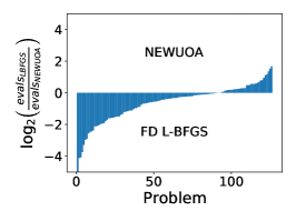
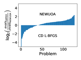
Figure 1: Efficiency, Noiseless Case. Log-ratio profiles for the total number of function evaluations to achieve (2.7) with $\epsilon(x)=0$. The left figure compares forward-difference l-bfgs with newuoa, and the right figure compares central-difference l-bfgs with newuoa.

In order to illustrate iteration cost, we report in Table 1 the CPU times for newuoa and l-bfgs for a representative problem as the number of variables $n$ increases. newuoa’s execution time grows much faster than l-bfgs because one iteration of newuoa requires $O(n^{2})$ flops, whereas the iteration cost of l-bfgs is $4tn$ flops, where $t=10$ and all test functions are inexpensive to evaluate. Across all the problems, we observe that when $n\approx 100$, newuoa can take at least $5-10$ times longer than l-bfgs in terms of wall-clock time.

$n$	10	20	30	50	90	100	500
NEWUOA	9.61e-2	9.99e-2	1.21e-1	1.99e-1	5.83e-1	8.92e-1	2.42e2
FD L-BFGS	1.13e-2	1.68e-2	2.26e-2	3.18e-2	5.50e-2	6.67e-2	4.67e-1
CD L-BFGS	1.30e-2	2.09e-2	2.90e-2	4.28e-2	6.63e-2	8.56e-2	6.63e-1

Table 1: Computing Time, Noiseless Case. CPU time (in seconds) required for newuoa and l-bfgs with forward (FD) and central (CD) differencing to satisfy (2.7) on the NONDIA problem, as the dimension of the problem $n$ increases.

While newuoa is an inherently sequential algorithm, finite-difference l-bfgs offers ample opportunities for parallelism when computing the finite-difference approximation to the gradient, which can be distributed across multiple nodes, with the only sequential bottleneck arising in the function evaluations within Armijo-Wolfe line search. Given the ratio between the number of function evaluations needed for newuoa versus finite-difference l-bfgs reported in Tables 4-8 in Appendix C.1.1, we hypothesize that even small amounts of parallelism across even a few processors may lead to significant speedup of l-bfgs. This is an often overlooked benefit of finite-difference-based methods in the DFO literature, as we are not aware of implementations of model-based trust-region methods that benefit significantly from parallelism.

We conclude this subsection by noting that most DFO methods were developed and tested primarily in the noiseless setting [18, 30]. Our results suggest that most of these methods may not be competitive with the finite-difference l-bfgs approach in the noiseless case. However, since no single set of experiments can conclusively establish such a claim, tests by other researchers should verify our observations.

2.2 Experiments on Noisy Functions

In this set of experiments, we synthetically inject uniform stochastic noise into the objective function. In particular, we sample $\epsilon(x)\sim\sigma_{f}U(-\sqrt{3},\sqrt{3})$ i.i.d. independent of $x$, where $\sigma_{f}\in\{10^{-1},10^{-3},10^{-5},10^{-7}\}$. (Thus, strictly speaking we should write $\epsilon$, but we keep the notation $\epsilon(x)$ for future generality.) By construction of $\epsilon(x)$, we have that $\sigma_{f}^{2}=\mathbb{E}[\epsilon(x)^{2}]$. We refer to standard deviation of the noise $\sigma_{f}$ as the noise level.

We employ a more precise formula for the finite-difference interval than in the noiseless setting — one that depends both on the noise level $\sigma_{f}$ and on the curvature of the function. Specifically, we compute a different $h_{i}$ for each coordinate direction based on the following well-known result [38] that provides bounds on the mean-squared error of estimated derivatives.

Theorem 2.1.

Let $h_{0}>0$ and $x,p\in\mathbb{R}^{n}$, with $\|p\|=1$, be given. Define the interval $I_{\text{FD}}=\{x+tp:t\in[0,h_{0}]\}$. If $|D_{p}^{2}\phi(y)|=|p^{T}\nabla^{2}\phi(y)p|\leq L$ for all $y\in I_{\text{FD}}$, then for any $\tilde{h}\in(0,h_{0}]$, the following bound holds for forward differencing:

$$\sigma_{g,p}(\tilde{h})^{2}\equiv\mathbb{E}\left[\left(g(x;p,\tilde{h})-D_{p}\phi(x)\right)^{2}\right]\leq\frac{L^{2}\tilde{h}^{2}}{4}+\frac{2\sigma_{f}^{2}}{\tilde{h}^{2}},$$ (2.9)

where

$$g(x;p,\tilde{h})=\frac{f(x+\tilde{h}p)-f(x)}{\tilde{h}}.$$ (2.10)

Similarly for central differencing, if the third derivative satisfies $|D_{p}^{3}\phi(y)|\leq M$ for all $y\in I_{\text{CD}}=\{x\pm tp:t\in[0,h_{0}]\}$, then for any $\tilde{h}\in(0,h_{0}]$ we have

$$\sigma_{g,p}(\tilde{h})^{2}\equiv\mathbb{E}[(g(x;p,\tilde{h})-D_{p}\phi(x))^{2}]\leq\frac{M^{2}\tilde{h}^{4}}{36}+\frac{\sigma_{f}^{2}}{2\tilde{h}^{2}},$$ (2.11)

where $D_{p}^{3}\phi(y)$ denotes the third directional derivative with respect to direction $p$ and

$$g(x;p,\tilde{h})=\frac{f(x+\tilde{h}p)-f(x-\tilde{h}p)}{\tilde{h}}.$$ (2.12)

By minimizing the upper bounds in (2.9), (2.11) with respect to $\tilde{h}$, one obtains the following expressions for each coordinate direction [38],

$$[g(x)]_{i} =\frac{f(x+h_{i}e_{i})-f(x)}{h_{i}}, h_{i}=\sqrt[4]{8}\sqrt{\frac{\sigma_{f}}{L_{i}}};$$ (forward differencing) (2.13)

$$[g(x)]_{i} =\frac{f(x+h_{i}e_{i})-f(x-h_{i}e_{i})}{2h_{i}}, h_{i}=\sqrt[3]{\frac{3\sigma_{f}}{M_{i}}},$$ (central differencing) (2.14)

where $L_{i}$ and $M_{i}$ are bounds on the second and third derivative along the $i$-th coordinate direction $e_{i}$. The noise level of the derivative along an arbitrary direction $p\in\mathbb{R}^{n}$ can be shown to be

$$\sigma_{g,p}\leq\sqrt[4]{2}\sqrt{L\sigma_{f}}\qquad\sigma_{g,p}\leq\frac{\sqrt[6]{3}}{2}M^{1/3}\sigma_{f}^{2/3},$$

for forward and central differencing, respectively. For the full gradient, the mean-squared error is given by

$$\sigma_{g}^{2}\equiv\mathbb{E}[\|g(x)-\nabla\phi(x)\|^{2}]=\sum_{i=1}^{n}\sigma_{g,e_{i}}^{2}.$$ (2.15)

With the formulas (2.13), (2.14) in hand, we can now return to the practical implementation of the finite-difference l-bfgs method. We estimate the constants $L_{i}$ in (2.13) using a second-order difference. Given a direction $p\in\mathbb{R}^{n}$ where $\|p\|=1$, we define

$$\Delta(t)=f(x+tp)-2f(x)+f(x-tp),$$

where $t$ is the second-order differencing interval. The Lipschitz constant $L$ along the direction $p$ can thus be approximated as $L\approx\Delta(t)/t^{2}$. However, as with the choice of $h$, we need to be careful in the selection of $t$, and for this purpose we employ an iterative technique proposed by Moré and Wild [38], whose goal is to find an interval $t$ that satisfies

$$|\Delta(t)| \geq\tau_{1}\epsilon_{f}, \tau_{1}\gg 1$$ (2.16)

$$|f(x\pm tp)-f(x)| \leq\tau_{2}\max\{|f(x)|,|f(x\pm tp)|\}, \tau_{2}\in(0,1).$$ (2.17)

These heuristic conditions aim to ensure that $t$ is neither too small nor too large; see [38] for a full description of the Moré-Wild (MW) technique. This technique cannot, however, be guaranteed to find a $t$ that satisfies (2.16), (2.17). To account for this, we developed the following procedure for estimating the constants $L_{i}$ for forward differencing.

Procedure I. Adaptive Estimation of $L$

1. At the first iteration of the l-bfgs method, invoke the MW procedure to compute $t_{i}$, for $i=1,...,n$. If such a $t_{i}$ can be found to satisfy (2.16), (2.17), set $L_{i}=\max\{10^{-1},|\Delta(t_{i})|/t_{i}^{2}\}$ in (2.13). Otherwise, set it to $L_{i}=10^{-1}$. Store the $L_{i}$ in a vector $\mathbf{L}$. To calculate the directional derivative in the Armijo-Wolfe line search, set the second-order differencing interval to $t=\|{\bf L}\|/\sqrt{n}$.

2. If at any iteration of the l-bfgs algorithm the line search returns a steplength $\alpha_{k}<0.5$, then re-estimate the vector $\mathbf{L}$ by calling the MW procedure as in step 1 at the current iterate $x_{k}$.

When the gradient is sufficiently accurate, l-bfgs generates well-scaled directions such that $\alpha_{k}=1$ is acceptable. Thus, the occurrence of $\alpha_{k}<0.5$ is viewed as an indication that the curvature of the problem may have changed, and should be re-estimated. The function evaluations performed in the estimation of $\mathbf{L}$ will be accounted for in the numerical results presented below.

For central differencing, a practical procedure for estimating $M$ is more involved, and will be discussed in a forthcoming paper [54]. Here, we simply approximate $M$ using changes in the second derivative of the true objective:

$$M=\max\left\{10^{-1},\frac{\left|p^{T}\left(\nabla^{2}\phi\left(x+\hat{h}\frac{p}{\|p\|}\right)-\nabla^{2}\phi(x)\right)p\right|}{\hat{h}\|p\|^{2}}\right\}$$ (2.18)

where $\hat{h}=\sqrt{\epsilon_{M}}$. This is an idealized strategy, and its cost is not accounted for in the results below since central differencing does not play a central role in this study.

In addition to the choice of $h$ mentioned above, we have found it important to modify the line search slightly to better handle noise. Following Shi et al. [53], we relax the Armijo condition within the Armijo-Wolfe line search, as follows. Let the superscript $j$ denote the $j$th iteration of the line search performed from the iterate $x_{k}$. The modified Armijo condition is

$$f(x_{k}+\alpha_{k}^{j}p_{k})\leq\begin{cases}f(x_{k})+c_{1}\alpha_{k}^{j}g(x_{k})^{T}p_{k}&\mbox{ if }j=0,\,g(x_{k})^{T}p_{k}<-\sigma_{g}\|p_{k}\|\\ f(x_{k})+c_{1}\alpha_{k}^{j}g(x_{k})^{T}p_{k}+2\sigma_{f}&\mbox{ if }j\geq 1,\,g(x_{k})^{T}p_{k}<-\sigma_{g}\|p_{k}\|\\ f(x_{k})&\mbox{ if }g(x_{k})^{T}p_{k}\geq-\sigma_{g}\|p_{k}\|.\end{cases}$$ (2.19)

Other than this modification to the line search, no other changes are made to the l-bfgs method. We will refer to the resulting method simply as l-bfgs to avoid introducing more acronyms.

We perform tests to compare l-bfgs with forward and central differencing against newuoa, both in terms of the achievable solution accuracy and in terms of efficiency (as measured by function evaluations).

2.2.1 Accuracy

We first compare the accuracy achieved by each algorithm, as measured by the optimality gap $\phi(x_{k})-\phi^{*}$. We do so by running newuoa until $\rho=\rho_{\text{end}}=10^{-6}$, and running the finite-difference l-bfgs method until the objective function could not be improved over 5 consecutive iterations. In Figure 2, we report the log-ratio profile

$$\log_{2}\left(\frac{\phi_{\text{\sc lbfgs}}-\phi^{*}}{\phi_{\text{\sc newuoa}}-\phi^{*}}\right)$$ (2.20)

for $\sigma_{f}=10^{-5}$, where $\phi_{\text{\sc lbfgs}}$, $\phi_{\text{\sc newuoa}}$ denote the lowest objective achieved by each method. (The results are representative of those obtained for $\sigma_{f}\in\{10^{-1},10^{-3},10^{-7}\}$.) As in the noiseless case, we removed 4 problems where newuoa terminates within the first $2n+1$ function evaluations for all noise levels, as well as thirteen problems where the algorithms are known to converge to different minimizers without noise.

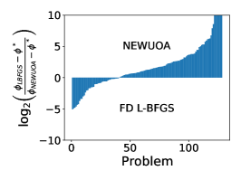
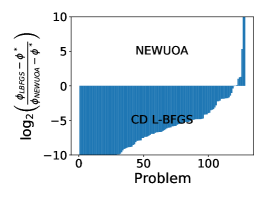
Figure 2: Accuracy, Noisy Case for $\sigma_{f}=10^{-5}$. Log-ratio optimality gap profiles comparing newuoa against forward-difference l-bfgs (left) and central-difference l-bfgs (right).

As seen in Figure 2, newuoa achieves higher accuracy in the solution than forward-difference l-bfgs, while central-difference l-bfgs yields far better accuracy than both. It is not surprising that central differencing yields much higher accuracy than forward differencing since the noise level of their gradient approximations is, respectively, $O(\sigma_{f}^{2/3})$ and $O(\sigma_{f}^{1/2})$. On the other hand, it is not straightforward to analyze the error contained in the gradient approximation constructed by newuoa, and in turn its final accuracy. To try to shed some light into this question, we performed the following experiments.

Recall that newuoa by default uses $p=2n+1$ interpolation points when constructing the quadratic model of the objective, while forward differencing only uses $n+1$ points. It is then natural to test the performance of newuoa with only $p=n+2$ interpolation points. The results in Figure 3 show that newuoa now lags behind finite-difference l-bfgs, which may be due the fact that the quality of its gradient also depends on the poisedness of the interpolation set [18, 8, 9]. Additional tests, given in Appendix B, suggest that the choice $p=2n+1$ recommended by Powell strikes the right balance between accuracy in the solution and the speed of algorithm.

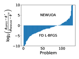
Figure 3: Accuracy for Non-Default Version of newuoa, Noisy Case for $\sigma_{f}=10^{-5}$. Log-ratio optimality gap profiles comparing newuoa with $p=2n+1$ and $p=n+2$ points (left), and newuoa with $p=n+2$ points against forward-difference l-bfgs (right).

It has been commonly suggested that estimating the Lipschitz constant $L_{i}$ along each coordinate at the initial point is sufficient for the entire run of a finite-difference method [23, 38]. This, in fact, is not the case in our experiments. We compare in Figure 4 forward-difference l-bfgs with the adaptive Lipschitz estimation given in Procedure I against estimating $L$ only once at the beginning of the run. We see that, in terms of solution accuracy, fixing the Lipschitz constant $L$ at the start does not yield nearly as good accuracy as the adaptive procedure. This is because that initial estimate is often not a proper bound on the second derivative in the later stages of the run, hence yielding a poor estimate of the finite-difference interval $h$, and consequently greater error in the gradient approximation. A variety of other strategies for estimating $L$ are discussed in Appendix A.

Figure 4: Accuracy of Fixed and Adaptive Lipschitz Estimation for l-bfgs, Noisy Case for $\sigma_{f}=10^{-5}$. Log-ratio optimality gap profiles comparing fixed Lipschitz estimates against adaptive Lipschitz estimation for forward-difference l-bfgs.

2.2.2 Efficiency

To compare the efficiency of different algorithms, we record the number of function evaluations required to reach a particular function value. We use the best solution from newuoa (denoted by $\phi_{new}$) as a baseline and report the number of function evaluations necessary to achieve

$$\phi(x_{k})-\phi_{new}\leq\tau\cdot(\phi(x_{0})-\phi_{new}),$$ (2.21)

for varied $\tau$. In Figure 5, we report log-ratio profiles comparing the number of function evaluations necessary to satisfy (2.21), i.e.,

$$\log_{2}\left(\frac{\mbox{${\rm evals}_{\mbox{{\rm\tiny LBFGS}}}$}}{\mbox{${\rm evals}_{\mbox{{\rm\tiny NEWUOA}}}$}}\right).$$ (2.22)

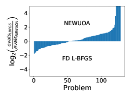
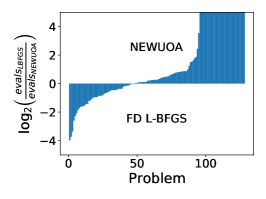
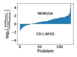
Figure 5: Efficiency, Noisy Case for $\sigma_{f}=10^{-5}$. Log-ratio profiles for the number of function evaluations to achieve (2.21) for $\tau=10^{-2}$ (left) and $10^{-6}$ (right), comparing newuoa against forward-difference l-bfgs (top) and central-difference l-bfgs (bottom). These plots are representative of the other noise levels $\sigma_{f}\in\{10^{-1},10^{-3},10^{-5},10^{-7}\}$.

We observe from this figure that newuoa is more efficient than forward-difference l-bfgs. The advantage is less significant for $\tau=10^{-2}$ but becomes pronounced for $\tau=10^{-6}$, which is to be expected because, as mentioned above, the forward-difference option struggles to achieve as high accuracy as newuoa. Central-difference l-bfgs is also less efficient overall than newuoa, but becomes more competitive as $\tau$ is decreased, which is a product of its ability to converge to a higher accuracy than forward differencing. It is notable that newuoa is able to deliver such strong performance without knowledge of the noise level of the function. The adjustment of the two trust-region radii in newuoa seems to be quite effective: shrinking the radii fast enough to ensure steady progress, but not so fast as to create models dominated by noise. To our knowledge, there has been no in-depth study of the practical behavior of newuoa (or similar codes) in the presence of noise; we regard this as an interesting research topic.

We also compare the efficiency of newuoa with only $p=n+2$ interpolation points against forward-difference l-bfgs; see Figure 6. We observe that forward-difference l-bfgs is more competitive in this case. More details are given in Appendix B.

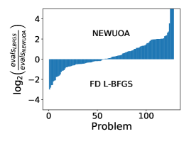
Figure 6: Efficiency for Non-Default Version of newuoa, Noisy Case. Log-ratio profiles for the number of function evaluations to achieve (2.21) for $\tau=10^{-2}$ (left) and $10^{-6}$ (right) for $\sigma_{f}=10^{-5}$ comparing newuoa with $p=n+2$ interpolation points against forward-difference l-bfgs.

One conclusion from these results is that a more sophisticated implementation of finite differences is required to close the performance gap between l-bfgs and newuoa. This requires a more accurate, yet affordable, mechanism for estimating the Lipschitz constants in the course of the run. The design of an adaptive procedure of this kind is the subject of a forthcoming paper [54]. It must be able to deal with some of the challenging situations described next.

2.2.3 Commentary

It is well known in computational mathematics that finite-difference methods can be unreliable in the solution of differential equations when knowledge of higher-order derivative estimates is poor. Optimization, however, provides a more benign setting in that a poor choice of $h$ that leads to a bad step can, in many situations, be identified and corrective action can be taken. Gill et al. [23] propose an iterative procedure for estimating $h$, but we believe that more sophisticated strategies must be developed to improve the reliability of finite-difference DFO methods. The design of such techniques is outside the scope of this paper, but we now give one example illustrating the challenges that arise and some opportunities for addressing them.

Let us consider the use of forward differences for the solution of the DENSCHNE problem from the CUTEst collection, which is given by

$$\min_{x\in\mathbb{R}^{3}}\phi(x)=x_{1}^{2}+(x_{2}+x_{2}^{2})^{2}+(-1+e^{x_{3}})^{2},\leavevmode\nobreak\ \leavevmode\nobreak\ \leavevmode\nobreak\ \text{with }x_{0}=(2,3,-8).$$

Let us employ a different interval for each variable, and let us focus in particular on $x_{3}$. The choice of the differencing interval $h_{3}$ depends on an estimate $L$ of the second derivative. We have that

$$\frac{\partial\phi}{\partial x_{3}}(x) =2e^{x_{3}}(e^{x_{3}}-1),\qquad\frac{\partial^{2}\phi}{\partial x_{3}^{2}}(x)=2e^{x_{3}}(2e^{x_{3}}-1).$$

Let us define $L$ to be the value of the second derivative at $x_{3}=-8$. This gives $L=\frac{2e^{8}-4}{e^{16}}\approx 6.705\times 10^{-5}$, which reflects the fact that $\phi$ is very flat at that point. Suppose that the noise level is $\sigma_{f}=10^{-1}$, then from (2.13), we have that $h\approx 20.539$, which is excessively long given that the function contains an exponential term. The forward-difference derivative approximation, $[g(x)]_{3}\approx 3.791\times 10^{9}$, is entirely wrong; the correct value is $[\nabla\phi(x)]_{3}=2e^{-8}(e^{-8}-1)\approx-6.707\times 10^{-4}$. Clearly, the problem is caused by the fact that the second derivative changes rapidly in the interval $[-8,-8+20.539]$ and we employed its lowest instead of its largest value. By greatly underestimating $L$ we computed an harmful differencing interval. (We should note in passing that newuoa does not have any difficulties with the DENSCHNE problem.)

However, the difficulties arising in this problem can be prevented at two levels. First, it should be possible to design an automatic procedure similar to the one in Gill et al. [23] that would not allow for the creation of such a poor estimate of $h$. In particular, the procedure should estimate $L$ along an interval, not just in a pointwise fashion. Even if such a procedure is unable to take corrective action, monitoring the optimization step can identify difficulties. For the example given above, the fact that $g(x)$ is huge causes the algorithm to compute a very small steplength $\alpha_{k}$. This gives a warning signal that should cause an examination of the interval $h$, and would immediately reveal that the second derivative has varied rapidly in the differencing interval and that $L$ must be recomputed.

It is easy to envision problems where the finite-difference interval $h$ is underestimated, in which case the effect of noise can be damaging. In addition, one must ensure that automatic procedures for estimating and correcting $L$ are not too costly. Taken, all together, these challenges motivate research into more reliable techniques for finite-difference estimation, in the context of optimization.

3 Nonlinear Least Squares

In many unconstrained optimization problems, the objective function has a nonlinear least-squares form. Therefore, it is important to pay particular attention to this problem structure in the derivative-free setting. We write the problem as

$$\min_{x\in\mathbb{R}^{n}}\phi(x)=\tfrac{1}{2}\|\gamma(x)\|^{2}=\tfrac{1}{2}\sum_{i=1}^{m}\gamma_{i}^{2}(x),$$

where $\gamma:\mathbb{R}^{n}\rightarrow\mathbb{R}^{m}$ is a smooth function. We assume that the Jacobian matrix $[J(x)]_{ij}=\frac{\partial\gamma_{i}(x)}{\partial x_{j}}$ is not available, but the individual residual functions $\gamma_{i}(x)$ can be computed. More generally, the evaluation of the $\gamma_{i}$ may contain noise so that the observed residuals are given by

$$r_{i}(x)=\gamma_{i}(x)+\epsilon_{i}(x),\quad i=1,\ldots,m,$$

where $\epsilon_{i}(x)$ models noise as in (2.1). Thus, the minimization of the true objective function $\phi$ must be performed based on noisy observations $r_{i}(x)$ that define the observed objective function

$$f(x)=\tfrac{1}{2}\|r(x)\|^{2}=\tfrac{1}{2}\sum_{i=1}^{m}r_{i}^{2}(x).$$ (3.1)

Since noise is incorporated into each residual function, the model of noise is different from additive noise model in the general unconstrained case discussed in the previous section. In particular, the function evaluation $f(x)=\tfrac{1}{2}\sum_{i=1}^{m}\gamma_{i}^{2}(x)+2\epsilon_{i}(x)\gamma_{i}(x)+\epsilon_{i}^{2}(x)$ contains both multiplicative and additive components of noise.

Our goal is to study the viability of methods based on finite-difference approximations to the Jacobian. To this end, we employ a classical Levenberg-Marquardt trust-region method where the Jacobian is approximated by differencing, and perform tests comparing it against a state-of-the-art DFO code designed for nonlinear least-squares problems. The rationale behind the selection of codes used in our experiments is discussed next.

Interpolation Based Trust Region Methods.

Wild [55] proposed an interpolation-based trust-region method that creates a quadratic model for each of the residual functions $\gamma_{i}$, and aggregates these models to obtain an overall model of the objective function. This method has been implemented in pounders [55, 39], which has proved to be significantly faster than the standard approach that ignores the nonlinear least-squares structure and simply interpolates values of $f$ to construct a quadratic model. Zhang, Conn and Scheinberg [57] describe a similar method, implemented in dfbols, where each residual function is approximated by a quadratic model using $p\in[n+1,(n+1)(n+2)/2]$ interpolation points; the value $p=2n+1$ being recommended in practice.

More recently, Cartis and Roberts [51] proposed a Gauss-Newton type approach in which an approximation of the Jacobian $J(x_{k})$ is computed by linear interpolation using $n+1$ function values at recently generated points $Y_{k}=\{x_{k},y_{1},...,y_{n}\}$. Here $x_{k}$ is the current iterate, which generally corresponds to the smallest objective value observed so far. The approximation $\hat{J}(x_{k})$ of the true Jacobian $J(x_{k})$ is thus obtained by solving the linear equations

$$r(x_{k})+\hat{J}(x_{k})(y_{j}-x_{k})=r(y_{j}),\quad j=1,...,n.$$ (3.2)

The step of the algorithm $s_{k}$ is defined as an approximate solution of the trust region problem

$$\min_{s\in\mathbb{R}^{n}}\ m_{k}(s)=f(x_{k})+g_{k}^{T}s+\tfrac{1}{2}s^{T}H_{k}s\qquad\mbox{s.t.}\ \ \|s\|_{2}\leq\Delta_{k},$$

where $g_{k}=\hat{J}(x_{k})^{T}r(x_{k})$ and $H_{k}=\hat{J}(x_{k})^{T}\hat{J}(x_{k})$. The new iterate is given by $x_{k+1}=x_{k}+s_{k}$ and the new set $Y_{k+1}$ is updated by removing a point in $Y_{k}$ and adding $x_{k+1}$. As in all model-based interpolation methods, it is important to ensure that the interpolation points do not lie on a subspace of $\mathbb{R}^{n}$ (or close to a subspace). To this end, the algorithm contains a geometry improving technique that spaces out interpolation points, as needed. The implementation described in [51], and referred to as dfo-gn, is reported to be faster than pounders, and scales better with the dimension of the problem. An improved version of dfo-gn is dfo-ls [12], which provides a variety of options and heuristics to accelerate convergence and promote a more accurate solution. The numerical results reported by Roberts et al. [12] indicate that dfo-ls is a state-of-the-art code for DFO least squares, and therefore will be used in our benchmarking.

Finite-Difference Gauss-Newton Method.

One can employ finite differencing to estimate the Jacobian matrix $J(x)$ within any method for nonlinear least squares, and since this is a mature area, there are a number established solvers. We chose lmder for our experiments, which is part of the MINPACK package [35] and is also available in the scipy library. We did not employ lmdif, the finite-difference version of lmder, because it does not allow the use of different differencing intervals for each of the residual functions $r_{i}(x)$; we elaborate on this point below. Another code available in scipy is trf [10], but our tests show that lmder is slightly more efficient in terms of function evaluations, and tends to give higher accuracy in the solution. The code nls, recently added to the Galahad library [24] would provide an interesting alternative. That method, however, includes a tensor to enhance the Gauss-Newton model, and since this may give it an advantage over dfo-ls, we decided to employ the more traditional code lmder.

In summary, the solvers used in our tests are:

• LMDER: A derivative-based Levenberg-Marquardt trust-region algorithm from the MINPACK software library [35], where the finite-difference module is user-supplied by us. We called the code in Python 3.7 through scipy version 1.5.3, using the default parameter settings.

• DFO-LS: The most recent DFO software developed by Cartis et al. [12] for nonlinear least squares. This method uses linear interpolation to construct an approximation to the Jacobian matrix, which is then used in a Gauss-Newton-type method. We used version 1.0.2 in our experiments, with default settings except that the model.abs_tol parameter is set to 0 to avoid early termination

The test problems in our experiments are those used by Moré and Wild [36], which have also been employed by Roberts and Cartis [51] and Zhang et al. [57]. The 53 unconstrained problems in this test set include both zero and nonzero residual problems, with various starting points, and are all small dimensional, with $n\leq 12$. To measure efficiency, we regard $m$ evaluations of individual residual components, say $\{r_{i}(\cdot)\}_{i=1}^{m}$, as one function evaluation. These $m$ evaluations may not necessarily be performed at the same point. We also assume that one can compute any component $r_{i}$ without a full evaluation of the vector $r(x)$. We terminate the algorithms when either: i) the maximum number of function evaluations ($500\times n$) is reached, ii) an optimality gap stopping condition, specified below, is triggered; or iii) the default termination criterion of the two codes is satisfied with tolerance of $10^{-8}$ (this controls the minimum allowed trust region radius).

3.1 Experiments on Noiseless Functions

We first consider the deterministic case corresponding to $\epsilon_{i}(x)\equiv 0,\,\forall i$. For lmder, we estimate the Jacobian $J(x)$ using forward differences. As before, let $\epsilon_{M}$ denote machine precision. We first evaluate $\{r(x+h_{j}e_{j})\}_{j=1}^{n}$, where

$$h_{j}=\max\{1,|[x]_{j}|\}\sqrt{\epsilon_{M}},$$

and compute the Jacobian estimate as

$$[\hat{J}(x)]_{ij}=\frac{r_{i}(x+h_{j}e_{j})-r_{i}(x)}{h_{j}}.$$

This formula for $h_{j}$ does not include a term that approximates the size of the second derivative (c.f.(2.13)) because we observed that such a refinement is not crucial in our experiments with noiseless functions, and our goal is to identify the simplest formula for $h$ that makes a method competitive.

As in the previous section, we consider log-ratio profiles to compare the efficiency and accuracy of lmder and dfo-ls. We record

$$\log_{2}\left(\frac{\text{evals}_{\text{\sc dfols}}}{\text{evals}_{\text{\sc lmder}}}\right)\quad\text{and}\quad\log_{2}\left(\frac{\phi_{\text{\sc dfols}}-\phi^{*}}{\phi_{\text{\sc lmder}}-\phi^{*}}\right),$$

where $\phi^{*}$ is obtained from [51], $\phi_{\text{\sc dfols}},\,\phi_{\text{\sc lmder}}$ denote the best function values achieved by the respective methods, and $\text{evals}_{\text{\sc dfols}},\,\text{evals}_{\text{\sc lmder}}$ denote the number of function evaluations needed to satisfy the termination test

$$\phi(x_{k})-\phi^{*}\leq\tau\max\{1,|\phi^{*}|\},$$ (3.3)

for various values of $\tau$. (We set $\text{evals}_{\text{\sc dfols}}$ and $\text{evals}_{\text{\sc lmder}}$ to be a very large number if the above condition is not achieved within the maximum number of function evaluations). The results comparing dfo-ls and lmder are summarized in Figures 7 and 8. The complete table of results is given in Appendix C.2.1.

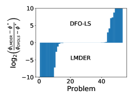
Figure 7: Accuracy, Noiseless Case. Log-ratio optimality gap profiles comparing dfo-ls and lmder for $\epsilon(x)=0$.

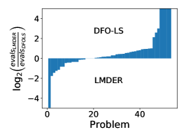
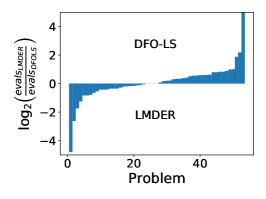
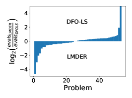
Figure 8: Efficiency, Noiseless Case. Log-ratio profiles comparing dfo-ls and lmder for $\epsilon(x)=0$. The figures measure number of function evaluations to satisfy (3.3) for $\tau=10^{-1}$ (left), $10^{-3}$ (middle), and $10^{-6}$ (right).

The performance of the two methods appears to be comparable since the area of the shaded regions is similar. This may be surprising since the Gauss-Newton approach seems to be a particularly effective way of designing an interpolation-based trust-region method, requiring only linear interpolation to yield useful second-order information. Cartis and Roberts [51] dismiss finite-difference methods at the outset, and do not provide numerical comparisons with them. However, the tradeoffs of the two methods merit careful consideration. dfo-ls requires only 1 function evaluation per iteration, but its gradient approximation, $\hat{J}(x_{k})^{T}r(x_{k})$, is inaccurate until the iterates approach the solution and the trust region has shrunk. In contrast, the finite-difference Levenberg-Marquardt method in lmder computes quite accurate gradients in this noiseless setting, requiring a much smaller number of iterations, but at a much higher cost per iteration in terms of function evaluations. The tradeoffs of the two methods appear to yield, in the end, similar performance, but we should note that dfo-ls is typically more efficient in the early stages of the optimization, as illustrated in Figure 8 for the low tolerance level $\tau=10^{-1}$. On the other hand, the finite-difference approach is more amenable to parallel execution, as mentioned in the previous section.

Let us now consider the linear algebra cost of the two methods. A typical iteration of dfo-ls computes the LU factorization of the matrix $[y_{1}-x_{k},...,y_{n}-x_{k}]$, and solves the interpolation system (3.2) for $n$ different right hand sides, at a per-iteration cost of $O(mn^{2})$ flops, assuming that $m>n$. (dfo-ls offers a number of options, such as regression, which my involve a higher cost, but we did not invoke those options.) The linear algebra cost of the finite-difference version of lmder described above is $O(mn)$ flops. Therefore, in terms of CPU time, lmder is faster than dfo-ls in our experiments involving inexpensive function evaluations. This is illustrated in Table 2 for a typical problem (BROWNAL) with varying dimensions $n$ and $m$.

$(n,m)$	(5,5)	(10,10)	(30,30)	(50,50)	(100,100)	(300,300)	(500,500)
lmder	0.002	0.003	0.01	0.017	0.046	0.302	0.982
dfo-ls	0.127	0.059	0.762	0.104	0.34	5.404	24.085

Table 2: Computing Time, Noiseless Case. CPU time (in seconds) required by dfo-ls and lmder with forward differencing to satisfy (3.3) for $\tau=10^{-6}$ on the BROWNAL function, as $n$ and $m$ increase.

3.2 Experiments on Noisy Functions

Let us assume that the noise model is the same across all residual functions, i.e., $\epsilon_{i}(x)$ are i.i.d. for all $i$. As in Section 2.2, we generate noise independently of $x$, following a uniform distribution, $\epsilon_{i}(x)\sim\sigma_{f}U(-\sqrt{3},\sqrt{3})$, with noise levels $\sigma_{f}\in\{10^{-1},10^{-3},10^{-5},10^{-7}\}$.

Differencing will be performed more precisely than in the noiseless case. Following [37], the forward-difference approximation of the Jacobian is defined as

$$[\hat{J}(x_{k})]_{ij}=\frac{r_{i}(x+h_{ij}e_{j})-r_{i}(x)}{h_{ij}},\ \text{ where }h_{ij}=8^{1/4}\left(\frac{\sigma_{f}}{L_{ij}}\right)^{1/2},$$ (3.4)

where $L_{ij}$ is a bound on $|e_{j}^{T}\nabla^{2}\gamma_{i}(x)e_{j}|$ within the interval $[x,x+h_{ij}e_{j}]$. To estimate $L_{ij}$ for every pair $(i,j)$, and at every iteration, would be impractical, and normally unnecessary. Several strategies can be designed to provide useful information at an acceptable cost. For concreteness, we estimate $L_{ij}$ once at the beginning of the run of lmder.

More concretely, we compute a different $h_{ij}$ for every residual function $\gamma_{i}$ and each coordinate direction $e_{j}$ at the starting point, and keep $h_{ij}$ constant throughout the run of lmder. To do so, we compute the Lipschitz estimates $\{L_{ij}\}$ for $i=1,...,m,j=1,...,n$ by applying the Moré-Wild (MW) procedure [38] described in the previous section to estimate the Lipschitz constant for function $\gamma_{i}$ along coordinate directions $e_{j}$. If the MW procedure fails, we set $L_{ij}=1$. The cost of computing the $L_{ij}$, in terms of function evaluations, is accounted for in the results reported below.

In dfo-ls, we did not employ restarts, and set the obj_has_noise option to its default value False, which also changes some trust-region-related parameters. We did so for two reasons. First, restarts introduce randomness, and as Cartis et al. [12] observed, can lead the algorithm to a different minimizer, making comparisons difficult. In addition, restarts are designed to allow the algorithm to make further progress as it reaches the noise level of the function.

Accuracy. We compare the best optimality gap achieved by lmder and dfo-ls. We run the algorithms using their default parameters (except that we set model.abs_tol = 0 for dfo-ls) until no further progress could be made. In Figure 9, we plot the log-ratio profiles

$$\log_{2}\left(\frac{\phi_{\text{\sc dfols}}-\phi^{*}}{\phi_{\text{\sc lmder}}-\phi^{*}}\right),$$ (3.5)

for noise levels $\sigma_{f}\in\{10^{-1},10^{-3},10^{-5},10^{-7}\}$.

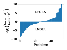
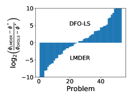
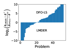
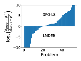
Figure 9: Accuracy, Noisy Case. Log-ratio optimality gap profiles comparing dfo-ls and lmder for $\sigma_{f}=10^{-1}$ (upper left), $10^{-3}$ (upper right), $10^{-5}$ (bottom left), $10^{-7}$ (bottom right). The bounds on the second derivatives are kept constant over the optimization process.

We observe that dfo-ls is more accurate than lmder, which points to the strengths of dfo-ls, since it does not require knowledge of the noise level of the function in its internal logic. However, our implementation of lmder is not sophisticated. As shown in the previous section, fixing the Lipschitz constant at the start of the finite-difference method is not always a good strategy, and one can ask whether a more sophisticated Lipschitz estimation strategy would close the accuracy gap. To explore this question, we implemented an idealized strategy in which the Lipschitz estimation is performed as accurately as possible. For every $(i,j)$, $L_{ij}$ is computed at every iteration, using true function information, via the formula

$$L_{ij}=\frac{|\gamma_{i}(x+he_{j})+\gamma_{i}(x-he_{j})-2\gamma_{i}(x)|}{h^{2}},\quad\mbox{with}\ h=(\epsilon_{M})^{1/4}.$$ (3.6)

We use this value in (3.4). The results are given in Figure 10, and indicate that lmder now achieves higher accuracy than dfo-ls on a majority of the problems across most noise levels. This highlights the importance of good Lipschitz estimates in the noisy settings, and suggests that the design of efficient strategies for doing so represent a promising research direction.

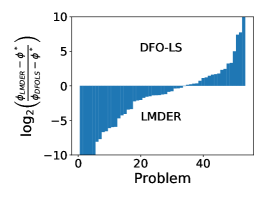
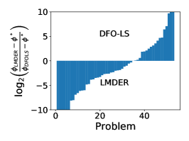
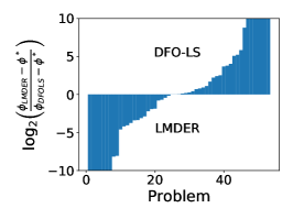
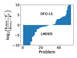
Figure 10: Accuracy with Idealized Lipschitz Estimation, Noisy Case. Log-ratio optimality gap profiles comparing dfo-ls and lmder for $\sigma_{f}=10^{-1}$ (upper left), $10^{-3}$ (upper right), $10^{-5}$ (bottom left), $10^{-7}$ (bottom right).

Efficiency. To measure the efficiency of the algorithms in the noisy case, we record the number of function evaluations required to satisfy the termination condition

$$\phi(x_{k})-\tilde{\phi}^{*}\leq\tau(\phi(x_{0})-\tilde{\phi}^{*}),$$ (3.7)

where $\tilde{\phi}^{*}$, denotes the best objective value achieved by the two solvers, for a given noise level. To do so, both solvers were run until they could not make more progress. The differencing interval in lmder was computed as in the experiments measuring accuracy for the noisy setting, i.e., by employing only the Moré-Wild procedure at the first iteration. In Figure 11, we plot

$$\log_{2}\left(\frac{\text{evals}_{\text{\sc dfols}}}{\text{evals}_{\text{\sc lmder}}}\right)$$ (3.8)

for three values of the tolerance parameter $\tau$ and for three levels of noise. We omit the plots for $\sigma_{f}=10^{-5}$, which demonstrate similar performance. (When (3.7) cannot be satisfied for a solver within the given budget of $500\times n$ function evaluations, we set the corresponding value in (3.8) to a very large number.)

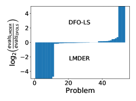
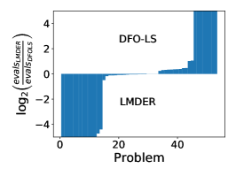
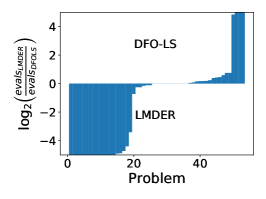
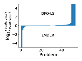
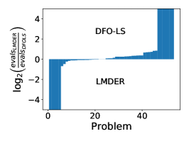
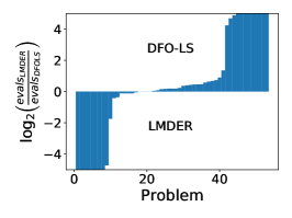
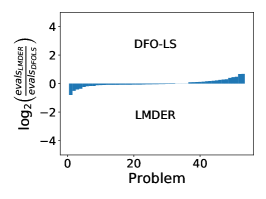
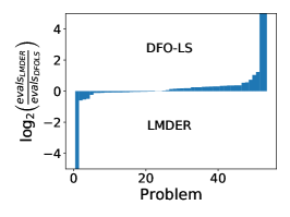
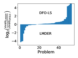
Figure 11: Efficiency, Noisy Case. Log-ratio profiles comparing dfo-ls and lmder for $\sigma_{f}=10^{-1}$ (top row), $10^{-3}$ (middle row), and $10^{-7}$ (bottom row). The figure measures the number of function evaluations to satisfy (3.3) for $\tau=10^{-1}$ (left column), $10^{-3}$ (middle column), and $10^{-6}$ (right column). Lipschitz constants were estimated only at the start of the lmder run.

There is no clear winner among the two codes used in the experiments reported in Figure 11. For low accuracy ($\tau=0.1$), lmder appears to be more efficient, whereas the opposite is true for high accuracy ($\tau=10^{-6}$). We note again that dfo-ls is able to handle different noise levels efficiently and reliably, without knowledge of the noise level or Lipschitz constants. On the other hand, the finite-difference approach is competitive even with a fairly coarse Lipschitz estimation procedure, and perhaps more importantly, it can be incorporated into existing codes (doing so in lmder required little effort). In other words, in the finite-difference approach to derivative-free optimization, algorithms do not need to be constructed from scratch but can be built as adaptations of existing codes.

3.2.1 Commentary

The nonlinear least squares test problems employed in our experiments are generally not as difficult as some of the unconstrained optimization problems tested in the previous section. This should be taken into consideration when comparing the relative performance of methods in each setting.

It is natural to question the necessity of estimating the Lipschitz constant for each component of each individual residual, as we did in our experiments, since this is affordable only if one can evaluate residual functions individually. One can envision problems for which a much simpler Lipschitz estimation suffices. For example, in data-fitting applications all individual residual functions $\gamma_{i}$ may be similar in nature. In this setting, one could use a single Lipschitz constant, say $L$, across all components and residual functions, especially when the variables are scaled prior to optimization. $L$ could be updated a few times in the course of the optimization process. If the scale of the variables varies signficantly, one can compute Lipschitz constants $L_{i}$ for each component across all residual functions, requiring the estimation of $n$ Lipschitz constants.

Another possibility is for the variables to be well scaled but the curvature of the residual functions $\gamma_{i}$ to vary signficantly. In this case, one could estimate the root mean square of the absolute value of the second derivatives for each component; see Appendix A. This approach notably only requires the estimation of a single constant for each residual function, yielding a total of $m$ Lipschitz constants. This permits the design of a more practical algorithm if the direct estimation of the root mean square is possible.

4 Constrained Optimization

We now consider inequality-constrained nonlinear optimization problems of the form

$$\min_{x\in\mathbb{R}^{n}}\phi(x)\qquad\mbox{s.t.}\ \ \psi(x)\leq 0,\quad l\leq x\leq u,$$ (4.1)

where $\psi:\mathbb{R}^{n}\rightarrow\mathbb{R}^{m}$ represents a set of $m$ linear or nonlinear constraints, $l,u\in\mathbb{R}^{n}$, and $\phi$ and $\psi$ are twice continuously differentiable. We assume that the derivatives of $\phi$ and $\psi$ are not available, and more generally that we have access only to noisy function evaluations:

$$f(x)=\phi(x)+\epsilon(x),\qquad c_{i}(x)=\psi_{i}(x)+\epsilon_{i}(x).$$ (4.2)

(We assume the same noise model for the objective $\epsilon$ and each of the constraint functions $\epsilon_{i}$, for simplicity.) In this section, we compare the numerical performance of an established DFO method designed to solve problem (4.1) against a standard method for deterministic optimization that approximates the gradients of the objective function and constraints through finite differences.

4.1 Choice of Solvers

The solution of constrained optimization problems using derivative-free methods has not been extensively studied in the literature; see the comprehensive review [30]. There are few established codes for solving problem (4.1) and even fewer for problems that contain both equality and inequality constraints. To our knowledge, the best known software for solving problem (4.1) is cobyla, developed by Powell [44]. The method implemented in that code constructs linear approximations to $\phi$ and $\psi$ at every iteration using function interpolation at points placed on a simplex in $\mathbb{R}^{n}$; it is designed to handle only inequality constraints. A more recent method by Powell, in the spirit of newuoa, is lincoa [45]. It implements an interpolation-based trust-region approach but it can handle only linear constraints. The nomad package by Abramson et al. [1] is designed to solve general constrained optimization problems. It is a direct-search method that employs a progressive barrier approach to handle the constraints, and builds quadratic models (or other surrogate functions) as a guide. In the numerical experiments reported in [2], cobyla outperforms nomad, and in [5], nomad is not among the best performing methods. Based on these results, we chose cobyla for our experiments.

There are many production-quality software packages for deterministic constrained optimization where we could implement the finite difference DFO approach. We chose knitro because one of the algorithms it offers is a simple sequential quadratic programming (SQP) method that is close in spirit to cobyla. We did not to employ the interior-point methods offered by knitro, which are known to be very powerful techniques for handling inequality constraints, because they may put cobyla at an algorithmic disadvantage. In the same vein, we did not employ snopt because it implements a sophisticated SQP method with many advanced features to improve efficiency and reliability. In short, we selected a simple nonlinear optimization method to more easily identify the strengths and weaknesses of the finite difference approach.

In summary, the codes tested are:

• COBYLA. We ran the version of cobyla maintained in the pdfo package [49]. We set the final trust region radius to $10^{-8}$ (rhoend=1e-8) to observe its asymptotic behavior, particularly in the noiseless case. We ran pdfo version 1.0, and called cobyla via its Python interface (Python 3.7.7).

• KNITRO. We ran Artelys Knitro 12.2 with alg=4 (an SQP algorithm), gradopt=2 (forward differencing), and hessopt=6 (L-BFGS). The choice of the finite difference interval $h$ is described below. In order to make the algorithm as close as possible to cobyla, we set the memory size of L-BFGS updating to its minimum value, $t=1$ (lmsize=1). For consistency with cobyla, we disabled the termination test based on the optimality error by setting opttol=1e-16, and findiff_terminate=0, and instead terminate when the computed step is less than $10^{-8}$ (by setting xtol=1e-8 and xtol_iters=1). We called knitro via its Python interface.

4.2 Test Problems

As in the previous sections, we used test problems from the CUTEst set [25], which were called through the Python interface, PyCUTEst version 1.0. We recall from (4.1) that $n$ and $m$ refer to the number of variables and constraints, respectively (excluding bound constraints). We first selected fixed-size problems that have at least one general nonlinear inequality and have no equality constraints, and for which $n\leq 100$ and $m\leq 100$. The properties of the resulting 49 problems are listed in Table 29 in Appendix C.3.1. We also selected 3 variable-size problems with at least one general nonlinear inequality and no equality constraints, and tested them with dimensions up to $n\leq 500$ and $m\leq 500$. These problems are listed in Table 30.

4.3 Experiments on Noiseless Functions

In the first set of experiments, we applied cobyla and knitro to solve the 49 small-scale, fixed-size CUTEst problems with exact function evaluations, i.e., with $\epsilon(x)=\epsilon_{i}(x)\equiv 0$ for all $i$. As in prior sections, the approximate gradient $g(x)\in\mathbb{R}^{n}$ of the objective function and Jacobian $\hat{J}(x)\in\mathbb{R}^{m\times n}$ of the constraints are evaluated by finite differencing:

$$[g(x)]_{i} =\frac{f(x+h_{i}e_{i})-f(x)}{h_{i}}$$ (4.3)

$$[\hat{J}(x)]_{ij} =\frac{c_{i}(x+h_{j}e_{j})-c_{i}(x)}{h_{j}}$$ (4.4)

where

$$h_{i}=\max\{1,|[x]_{i}|\}\sqrt{\epsilon_{M}},\quad i=1,...,n.$$ (4.5)

Both algorithms were stopped when the number of function evaluations exceed $500\max{(n,m)}$, or when the trust-region radius or steplength reaches its lower bound for cobyla or knitro, respectively. Both solvers report feasibility error as the max-norm of constraint violations.

Table 31 reports the results of these tests. A ^∗ indicates that the solver hits the limit of function evaluations. We sorted the results in Table 31 into four groups, separated by horizontal lines, according to the following outcomes:

(i) Both solvers converged to a feasible point with approximately the same objective function values.

(ii) The solvers converged to feasible points with different objective function values.

(iii) One of the solvers terminated at an infeasible point.

(iv) Both solvers terminated at infeasible points.

There were 32 problems associated with outcome (i). We can use them to safely compare the performance of the two solvers in terms of accuracy and efficiency. (We comment on outcomes (ii)-(iv) in Appendix C.3.2.)

Given that the two codes achieved feasibility in these 32 problems, we measure accuracy by comparing the best objective function value obtained by each solver with the value $\phi^{\ast}$ obtained by running knitro with exact gradients until it could not make further progress. (In all the runs for determining $\phi^{\ast}$, feasibility error was less than $10^{-10}$.) To measure accuracy, we report the ratios

$$\log_{2}\left(\frac{\max\{\phi_{\text{\tiny KNITRO}}-\phi^{\ast},10^{-8}\}}{\max\{\phi_{\text{\tiny COBYLA}}-\phi^{\ast},10^{-8}\}}\right).$$ (4.6)

We compare accuracy up to eight digits because reporting, say, the ratio $10^{-12}/10^{-15}$ would be misleading, given that the accuracy in the constraint violation could have the inverse ratio. The results are presented in Figure 12, which shows that for most problems both solvers were able to achieve eight digits of accuracy; for the remaining problems, knitro gave higher accuracy.

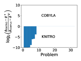
Figure 12: Accuracy, Noiseless Case. Log-ratio profiles comparing knitro and cobyla for $\epsilon(x)=\epsilon_{i}(x)=0$. The figure plots the ratios (4.6) for problems associated with outcome (i).

To measure efficiency, we conducted a series of experiments using the same subset of 32 problems corresponding to outcome (i). We record the number of function evaluations, $\text{evals}_{\text{\tiny KNITRO}}$ and $\text{evals}_{\text{\tiny COBYLA}}$, required by the two codes to satisfy the condition

$$\phi_{k}-\phi^{\ast}\leq\tau\cdot\max\{1,|\phi^{\ast}|\}$$ (4.7)

for various values of $\tau$. (If a solver fails to satisfy this test, we set the number of evaluations to a large value.) Figure 13 plots the ratios

$$\log_{2}\left(\frac{\text{evals}_{\text{\tiny KNITRO}}}{\text{evals}_{\text{\tiny COBYLA}}}\right)$$ (4.8)

for $\tau\in\{10^{-1},10^{-3},10^{-6}\}$. Table 32 contains the complete set of results. We observe that for low accuracy, cobyla is slightly more efficient, while knitro becomes significantly more efficient when high accuracy is required.

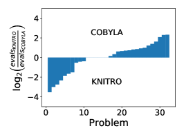
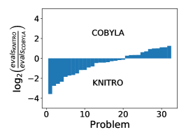
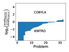
Figure 13: Efficiency, Noiseless Case. Log-ratio profiles comparing knitro and cobyla for $\epsilon(x)=\epsilon_{i}(x)=0$. The figures measure number of function evaluations to satisfy (4.7) for $\tau=10^{-1}$ (left), $10^{-3}$ (middle), and $10^{-6}$ (right) for outcome (i).

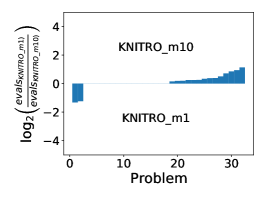
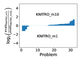
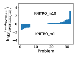
Figure 29: Efficiency, Noiseless Case. Log-ratio profiles comparing knitro with an l-bfgs Hessian approximation of memory one and memory 10 when $\epsilon(x)=0$. The figures measure number of function evaluations to satisfy (4.7) for $\tau=10^{-1}$ (left), $10^{-3}$ (middle), $10^{-6}$ (right).

We should note that employing memory size $t=1$ in L-BFGS updating yields a very weak quadratic model in the SQP method of knitro. We experimented with a memory of size $t=10$ and observed that the performance of knitro improved, particularly in the early iterations of the runs, but not dramatically; see Figure 29 in Appendix C.3.2.

Experiments on Variable-Dimension Problems without Noise. Next, we tested the two codes on the three problems of variable dimensions listed in Table 30, setting $\epsilon(x)=\epsilon_{i}(x)\equiv 0$. We impose a time limit of an hour; the runs exceeding the time limit are marked with a T. Table 3 displays the results. A clear picture emerges from these tests: knitro is more reliable than cobyla in terms of feasibility, tends to achieve a lower objective value, and can solve larger problems within the allotted time. We observed earlier that there is a perception in the DFO literature that finite differences require too many function evaluations, especially as the dimension of the problem increases. The results in Table 3 do not support that concern.

	KNITRO				COBYLA
problem	$\phi_{k}$	#evals	CPU time	feaserr	$\phi_{k}$	#evals	CPU time	feaserr
SVANBERGN10	15.7315	168	0.078	2.62E-14	26.0000	302	0.349	0.00E+00
SVANBERGN50	82.5819	950	0.538	4.11E-15	136.0000	2140	0.941	0.00E+00
SVANBERGN100	166.1972	1851	1.564	3.22E-15	273.5000	4715	9.754	0.00E+00
SVANBERGN500	835.1869	10054	76.771	1.50E-14	-	-	T	-
READING4N2	-0.0723	20	0.014	0.00E+00	-0.0723	50	0.165	0.00E+00
READING4N50	-0.2685	3556	1.767	8.22E-15	-0.0100	6099	0.123	3.61E+00
READING4N100	-0.2799	9957	16.043	8.44E-15	0.0163	8118	22.609	5.40E-01
READING4N500	-0.2893	88614	1198.368	6.00E-15	-	-	T	-
COSHFUNM3	-0.6614	379	0.152	3.77E-16	-0.6614	730	0.341	0.00E+00
COSHFUNM8	-0.7708	4673	1.424	2.22E-16	-0.7708	$12500^{*}$	0.324	0.00E+00
COSHFUNM14	-0.7732	$21500^{*}$	6.366	8.23E-13	-0.7731	$21500^{*}$	3.673	0.00E+00
COSHFUNM20	-0.7733	$30500^{*}$	10.792	5.42E-09	-0.7731	$30500^{*}$	8.430	0.00E+00

Table 3: Variable-Size Problems, Noiseless Case. Final objective value $\phi_{k}$, number of function evaluations (#evals), CPU time (in seconds), and final feasibility error (feaserr). A ^∗ indicates that the maximum number of function evaluations was reached, and T that the time limit (1 hour) was reached.

4.4 Experiments on Noisy Functions

We now inject artificial noise in the evaluation of the objective and constraint functions. We use the same noise model as in the unconstrained setting; i.e., uniform noise sampled i.i.d. given by

$$\epsilon(x),\epsilon_{i}(x)\sim\sigma_{f}U(-\sqrt{3},\sqrt{3}),$$

where $\sigma_{f}\in\{10^{-1},10^{-3},10^{-5},10^{-7}\}$. We use the same formulas for evaluating the finite-difference gradient (4.3) and Jacobian (4.4), but with a different formula for the finite-difference interval:

$$h_{i}=\max\{1,|[x]_{i}|\}\sqrt{\sigma_{f}},\quad i=1,...,n.$$

We do not include a Lipschitz constant because this formula will suffice for our purposes.

In the first experiment, we ran the two codes with their least stringent termination tests to observe the quality of the final solutions. As in the noiseless case, we set rhoend=1e-8 for cobyla and xtol=1e-8 for knitro, and impose a limit of $500\max\{n,m\}$ function evaluations. We tested the 32 CUTEst problems for which both solvers converged to the same feasible solution in the noiseless case (outcome (i) above). In Figure 14, we compare the accuracy $\phi(x_{k})-\phi_{\ast}$ in the true objective given by the code codes, up to eight digits, as in (4.6). If the feasibility violation is large compared to the noise level, i.e. $\|\max\{\psi(x_{k}),0\}\|_{\infty}\geq\sqrt{3}\sqrt{\sigma_{f}}$, we mark the corresponding run as a failure. We observe from Figure 14 that the performance of the two solvers is comparable, with knitro slightly more efficient for low accuracy. Interestingly, for the highest accuracy, $\sigma_{f}=10^{-7}$, the performance of the codes is remarkably close (note that the log ratio is nearly zero for about half of the problems). The complete set of results is given in Tables 33-38 in Appendix C.

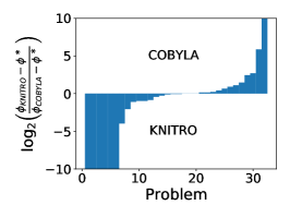
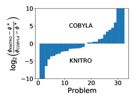
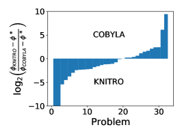
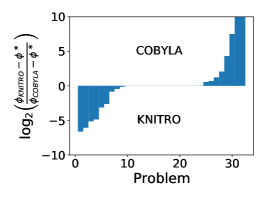
Figure 14: Accuracy, Noisy Case. Log-ratio profiles comparing accuracy in the objective by knitro and cobyla, for $\sigma_{f}=10^{-1}$ (upper left), $10^{-3}$ (upper right), $10^{-5}$ (bottom left), and $10^{-7}$ (bottom right).

Next, we compare the efficiency of the two solvers for two levels of accuracy in the objective. Specifically, we record the number of function evaluations required to satisfy

$$\phi(x_{k})-\tilde{\phi}_{\ast}\leq\tau(\phi(x_{0})-\tilde{\phi}_{\ast})\quad\mbox{and}\quad\|\max\{\psi(x_{k}),0\}\|_{\infty}\leq\sqrt{3}\sqrt{\sigma_{f}},$$ (4.9)

for $\tau\in\{10^{-2},10^{-6}\}$, where $\tilde{\phi}_{\ast}$ is the minimum objective value obtained by the two codes. Figure 15 plots the ratios (4.8), which suggest that it is difficult to choose between the two codes. Therefore, in our tests on noisy problems, an unsophisticated code (knitro/sqp) for deterministic nonlinear optimization, using a simple strategy for choosing the finite difference interval, is competitive with cobyla, a method specifically designed for derivative-free optimization.

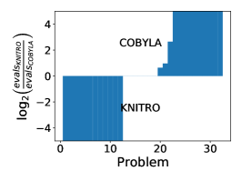
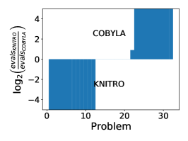
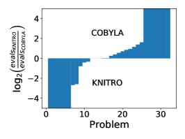
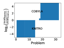
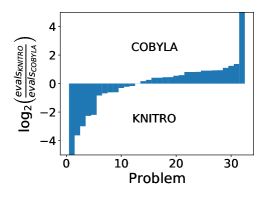
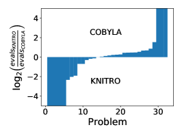
Figure 15: Efficiency, Noisy Case. Log-ratio profiles (4.8) comparing knitro and cobyla for $\sigma_{f}=10^{-1}$ (top row), $10^{-3}$ (middle row), $10^{-7}$ (bottom row). The figure measures the number of function evaluations to satisfy (4.9) for $\tau=10^{-2}$ (left) and $10^{-6}$ (right).

5 Final Remarks

Finite-difference approximations are widely employed within numerical analysis, particularly for solving ordinary and partial differential equations. The dangers and limitations of finite-difference methods are therefore also well-documented, such as the difficulty of approximating high-order derivatives accurately on unstructured grids or a failure to adapt to problems that require local mesh refinement.

Optimization, however, arguably provides a more benign setting than solving differential equations as errors do not accumulate; if a poor choice of the finite-difference interval yields a bad step, it can be detected and improved upon at a later point within the iteration. Two attractive features of finite-difference methods in optimization are the simplicity of incorporating them into existing nonlinear optimization solvers, and their ease of parallelization, in many situations.

Our empirical study has revealed that finite-difference methods can be made competitive, in many cases, against state-of-the-art derivative-free optimization methods. However, algorithmic development and analysis are still necessary to make them sufficiently robust for general-purpose optimization. In addition to more sophisticated procedures for computing the finite difference interval, research is needed in the design of globalization mechanisms such as line searches and trust regions in the noisy setting. We hope that our work draws attention to and provides an empirical basis for further investigation along this important line of inquiry.

Appendix A Numerical Investigation of Lipschitz Estimation

A.1 Investigation of Theoretical Lipschitz Estimates

In Section 2.2, we approximated the bound on the second and third derivative $L$ and $M$ (or the Lipschitz constant of the first and second derivative) along the interval $I=\{x\pm tp:t\in[0,h_{0}]\}$ for $h_{0}>0$ every time finite-differencing is performed.

For forward-differencing, we employed the Moré and Wild heuristic [38]. The heuristic estimates the bound on the second derivative of a univariate function with noise. Assume $\phi:\mathbb{R}\rightarrow\mathbb{R}$ is univariate. If we let $\Delta(t)=f(x+t)-2f(x)+f(x-t)$, then $t>0$ must satisfy two conditions:

$$|\Delta(t)| \geq\tau_{1}\epsilon_{f}, \tau_{1}\gg 1$$ (A.1)

$$|f(x\pm t)-f(x)| \leq\tau_{2}\max\{|f(x)|,|f(x\pm t)|\}, \tau_{2}\in(0,1).$$ (A.2)

In practice, $\tau_{1}=100$ and $\tau_{2}=0.1$. The first condition ensures that $h$ is sufficiently large such that the second-order difference is not dominated by noise, while the second condition enforces that the difference is not dominated by a particular evaluation, so that there is “equal” contribution from each function evaluation in the finite-difference approximation. If conditions (A.1) and (A.2) are satisfied, then we take $L=\max\{10^{-1},|\Delta(t)|/t^{2}\}$.

For central differencing, we used a theoretical estimate based on knowledge of the true Hessian $\nabla^{2}\phi(x)$:

$$M=\max\left\{10^{-1},\frac{|p^{T}(\nabla^{2}\phi(x+\tilde{h}\frac{p}{\|p\|})-\nabla^{2}\phi(x))p|}{\tilde{h}\|p\|^{2}}\right\}$$ (A.3)

where $\tilde{h}=\sqrt{\epsilon_{M}}$. Since this estimate is ideal, we do not include the cost of evaluating $M$ in the number of function evaluations. In both cases, the maximum is taken to ensure that the bound is strictly bounded away from $0$ so that (2.13) and (2.14) remain well-defined.

One may ask whether or not a refined choice of $L$ or $M$ is necessary for finite-difference l-bfgs. To show the impact of Lipschitz estimation on the performance of finite-difference methods, we focus on forward-difference l-bfgs and compare nine different theoretical Lipschitz estimation schemes. The first five consider techniques where $L$ is fixed for the entire run based on information at the initial point. We test this because it is frequently claimed that using an initial estimate of $L$ is sufficient for the entire run; see [23, 38]. The first approach requires no additional information about the function, while the others incorporate information about the Hessian at the current point. The latter four techniques similarly incorporate information about the Hessian but re-estimate $L$ whenever the finite-difference gradient or directional derivative is evaluated.

All of these techniques rely on the assumption that $|D_{p}^{2}\phi(x)|\approx|D_{p}^{2}\phi(\xi)|$ for some $\xi\in[x,x+h]$. As we will see, both of these approximations that are based on conventional wisdom are challenged in our experiments.

1. Fix $L=1$. This requires no additional knowledge about the problem at no added cost.

2. Fix $L=\max\{10^{-1},\|\nabla^{2}\phi(x_{0})\|_{2}\}$. Similar to fixing $L=1$, but incorporates knowledge of the initial Hessian.

3. Fix $L=\max\left\{10^{-1},\frac{1}{n}\sum_{i=1}^{n}|[\nabla^{2}\phi(x_{0})]_{ii}|\right\}$. This can be obtained by choosing $h$ such that the bound on $\|g(x_{0})-\nabla\phi(x_{0})\|_{1}$ at the initial point is minimized.

4. Fix $L=\max\left\{10^{-1},\frac{1}{\sqrt{n}}\sqrt{\sum_{i=1}^{n}[\nabla^{2}\phi(x_{0})]_{ii}^{2}}\right\}$. This can be obtained by choosing $h$ such that the bound on $\|g(x_{0})-\nabla\phi(x_{0})\|_{2}^{2}$ at the initial point is minimized.

5. Fix $L$ to a vector $(\max\{10^{-1},|[\nabla^{2}\phi(x_{0})]_{ii}|\})_{i=1}^{n}$ and use the $i$th component for estimating the $i$th component of $g(x)$. Uses $\|L\|_{2}/\sqrt{n}$ when estimating $h$ for the directional derivative in the line search.

6. Evaluate $L=\max\{10^{-1},\|\nabla^{2}\phi(x)\|_{2}\}$ each time finite-differencing is performed.

7. Evaluate $L=\max\left\{10^{-1},\frac{1}{n}\sum_{i=1}^{n}|[\nabla^{2}\phi(x)]_{ii}|\right\}$ each time finite-differencing is performed.

8. Evaluate $L=\max\left\{10^{-1},\frac{1}{\sqrt{n}}\sqrt{\sum_{i=1}^{n}[\nabla^{2}\phi(x)]_{ii}^{2}}\right\}$ each time finite-differencing is performed.

9. Evaluate $L=\max\left\{10^{-1},|[\nabla^{2}\phi(x)]_{ii}|\right\}$ when evaluating $[g(x)]_{i}$. When the directional derivative along $p\in\mathbb{R}^{n}$ is computed, evaluates $L=\max\left\{10^{-1},\frac{|p^{T}\nabla^{2}\phi(x)p|}{\|p\|_{2}^{2}}\right\}$ .

Each method is terminated when it cannot make more progress over 5 consecutive iterations. The optimal value $\phi^{*}$ is obtained by running l-bfgs on the non-noisy function until no more progress can be made.

To compare the solution quality between two algorithms, we will use log-ratio profiles as proposed in [34] over the optimality gaps for each algorithm. The log-ratio profiles report

$$\log_{2}\left(\frac{\phi_{\text{new}}-\phi^{*}}{\phi_{\text{old}}-\phi^{*}}\right)$$ (A.4)

for each problem plotted in increasing order. The area of the shaded region is representative of the general success of the algorithm.

One may ask whether or not using $L=1$ is sufficient, without any additional knowledge of the second derivative. As seen in Figure 16, when compared against the other fixed Lipschitz estimation schemes, the difference is not significant. In particular, the additional information from the Hessian does not yield significant benefits over setting $L=1$ because the bound on the second derivative does not remain valid over the entire run of the algorithm. This may be surprising as it has been commonly suggested that it is sufficient to fix the Lipschitz estimate; see [23, 38]. In fact, we will see that it is more crucial for the algorithm to have a right estimate of $L$ during the later stages of the run than at the beginning of the run in order to achieve high accuracy.

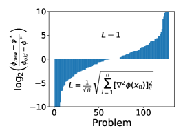
Figure 16: Accuracy, Noisy Case with $\sigma_{f}=10^{-3}$. Log-ratio optimality gap profiles comparing forward difference l-bfgs with $L=1$ and other fixed Lipschitz estimation schemes. The noise level is $\sigma_{f}=10^{-3}$, but is representative for $\sigma_{f}\in\{10^{-1},10^{-3},10^{-5},10^{-7}\}$.

To further support why an adaptive $L$ is important to achieve high accuracy, we compare the fixed $L$ approaches against the adaptive $L$ in Figure 17.

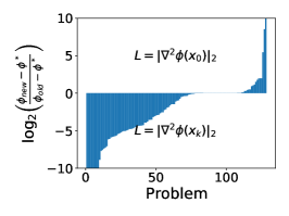
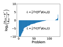
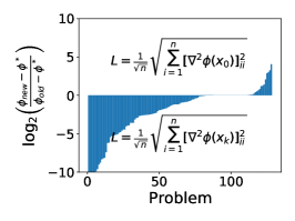
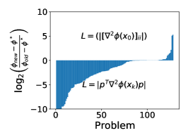
Figure 17: Accuracy, Noisy Case with $\sigma_{f}=10^{-3}$. Log-ratio optimality gap profiles comparing forward difference l-bfgs with fixed and adaptive Lipschitz estimation schemes. The noise level is $\sigma_{f}=10^{-3}$, but is representative for $\sigma_{f}\in\{10^{-1},10^{-3},10^{-5},10^{-7}\}$.

As seen in Figure 17, we see that using Lipschitz estimation at every iteration yields much higher accuracy than the alternatives. Upon inspection of individual runs, one can observe many cases where fixing the Lipschitz constant is unstable and inadequate, potentially leading to poor gradient approximations that result in early stagnation of the algorithm. This suggests that it is imperative to adaptively re-estimate $L$ in order to reduce the noise in the gradient and squeeze the best possible accuracy out of forward difference l-bfgs.

In addition, since estimating $L$ for each direction is most competitive out of the adaptive variants as seen in Figure 18, we present the results for a heuristic approach in our main work. However, our investigation reveals that the simple mean or root mean square can provide potentially cheaper alternatives if they can be estimated without knowledge of the componentwise Lipschitz constants.

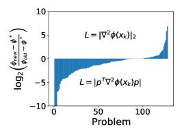
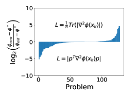
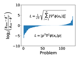
Figure 18: Accuracy, Noisy Case with $\sigma_{f}=10^{-3}$. Log-ratio optimality gap profiles comparing forward difference l-bfgs with fixed and adaptive Lipschitz estimation schemes. The noise level is $\sigma_{f}=10^{-3}$, but is representative for $\sigma_{f}\in\{10^{-1},10^{-3},10^{-5},10^{-7}\}$.

To our knowledge, there are two weaknesses with the componentwise estimation approach. The first is that for a small subset of problems, it is prone to underestimate the Lipschitz constant, as discussed in Section 2. The second weakness is that the approach, if performed at each iteration and approximated through finite-differencing, is far too expensive. We propose a few possible practical heuristics for handling this in the following section.

A.2 Practical Heuristics for Lipschitz Estimation

Two heuristics were proposed for estimating the Lipschitz constant. Moré and Wild [38] proposed a simple heuristic for estimating the bound on the second derivative of a univariate function with noise, as described in Section 2. Gill, et al. [23] proposed a similar procedure that instead enforces that the relative cancellation error lies within an interval

$$\frac{4\epsilon_{f}}{|\Delta(h)|}\in[0.001,0.1].$$ (A.5)

Note that the lower bound on the interval in (A.5) corresponds to (A.1).

Both of these heuristics were proposed with particular initial guesses of $h$ and additional conditions to handle certain cases where the methods can fail. These heuristics were employed only at the beginning of the iteration for each variable component, then remains fixed for the entire run.

The only work to our knowledge that employs re-estimation of the Lipschitz constant for finite-differencing derivative-free optimization is Berahas, et al. [7]. In his work, the Lipschitz constant is re-estimated whenever the line search fails and the recovery procedure is triggered. Similarly, we will use the Moré and Wild heuristic to estimate the Lipschitz constant, but only re-estimate the Lipschitz constant when $\alpha<0.5$ after the first iteration, as described in Procedure I in Section 2. We compare two variants of the Lipschitz estimation procedure:

1. Component MW: We use the Moré and Wild heuristic to estimate the Lipschitz constant with respect to each component. This is performed at the first iteration and subsequent iterations for line search methods when the line search from the prior iteration gives a steplength $\alpha_{k}<0.5$. When estimating the directional derivative along the search direction $p_{k}$, we use the root mean square of the component-wise estimates.

2. Random MW: We use the Moré and Wild heuristic to estimate the Lipschitz constant along a random direction sampled uniformly from a sphere, i.e., $p\sim S(0,I)$. This is performed at the first iteration and subsequent iterations for line search methods when the line search from the prior iteration gives a steplength $\alpha_{k}<0.5$.

We compare both Moré and Wild heuristics against newuoa and theoretical componentwise Lipschitz estimation in Figures 19, 20, and 21. In general, Component MW gives a better solution than Random MW. When we compare these methods against newuoa in Figure 21, the performance of the methods are relatively the same as the theoretical Lipschitz estimates.

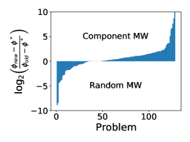
Figure 19: Accuracy, Noisy Case with $\sigma_{f}=10^{-3}$. Log-ratio optimality gap profiles comparing forward difference l-bfgs with component MW and random MW Lipschitz estimation schemes.

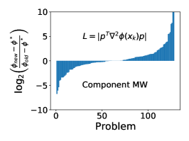
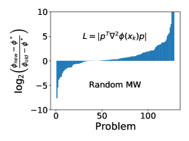
Figure 20: Accuracy, Noisy Case with $\sigma_{f}=10^{-3}$. Log-ratio optimality gap profiles comparing forward difference l-bfgs with theoretical componentwise Lipschitz estimates and the Moré and Wild Lipschitz estimation schemes.

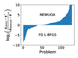
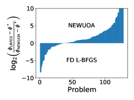
Figure 21: Accuracy, Noisy Case with $\sigma_{f}=10^{-3}$. Log-ratio optimality gap profiles comparing newuoa against forward difference l-bfgs with the Moré and Wild Lipschitz estimation schemes. We compare l-bfgs with Component MW (left) and Random MW (right).

Appendix B Investigation of Parameters for NEWUOA

In this section, we empirically investigate the influence of the parameters for newuoa for the noisy setting. Although these parameters have been optimized for the noiseless setting, it is not generally known how these parameters may impact its performance on noisy unconstrained problems. By default, newuoa employs $p=2n+1$ interpolation points when constructing the quadratic model at each iteration with an initial trust region radius of $\rho_{\text{beg}}=1$ and a final trust region radius of $\rho_{\text{end}}=10^{-6}$.

B.1 Number of Interpolation Points

In Section 2, we observed that newuoa is able to converge to a better quality neighborhood than l-bfgs with forward differencing, but inferior to central differencing. Since newuoa by default employs $p=2n+1$ points, it is natural to both ask if: (1) decreasing the number of interpolation points would yield a less accurate quadratic model, with a potentially less accurate gradient; and (2) increasing the number of points used in the interpolation may improve the accuracy of the solution to be competitive with central differencing.

To do this, we run newuoa with $p=n+2$ and $p=\min\left\{3n+1,\frac{(n+1)(n+2)}{2}\right\}$ interpolation points and compare their optimality gaps and number of function evaluations. In Figures 22 and 23, we report the log-ratio profiles for the objective function and function evaluations when comparing newuoa with $p=n+2$ and $p=2n+1$ points. We see that with higher noise levels, newuoa with $p=n+2$ tends to terminate earlier, while for lower noise levels, it is less efficient than newuoa with $p=2n+1$ points. In terms of solution quality, newuoa with $p=2n+1$ is able to converge to a higher accuracy in general than newuoa with $p=n+2$ points. This is similarly seen when we compare $p=3n+1$ and $p=2n+1$ points in Figures 24 and 25.

Figure 22: Noisy Case. Log-ratio optimality gap profiles comparing newuoa with $p=2n+1$ and $p=n+2$ points. The noise levels are $\sigma_{f}=10^{-1}$ (top left), $\sigma_{f}=10^{-3}$ (top right), $10^{-5}$ (bottom left), and $10^{-7}$ (bottom right).

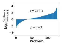
Figure 23: Noisy Case. Log-ratio function evaluation profiles comparing newuoa with $p=2n+1$ and $p=n+2$ points. The noise levels are $\sigma_{f}=10^{-1}$ (top left), $\sigma_{f}=10^{-3}$ (top right), $10^{-5}$ (bottom left), and $10^{-7}$ (bottom right).

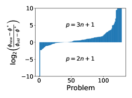
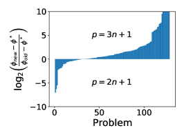
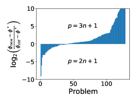
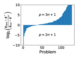
Figure 24: Noisy Case. Log-ratio optimality gap profiles comparing newuoa with $p=3n+1$ and $p=2n+1$ points. The noise levels are $\sigma_{f}=10^{-1}$ (top left), $\sigma_{f}=10^{-3}$ (top right), $10^{-5}$ (bottom left), and $10^{-7}$ (bottom right).

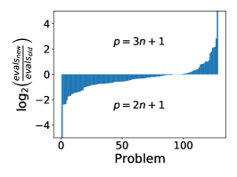
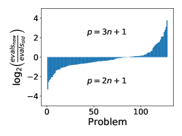
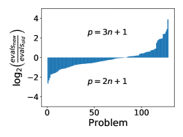
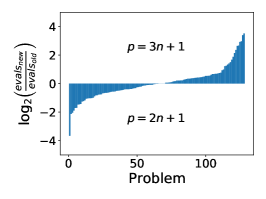
Figure 25: Noisy Case. Log-ratio function evaluation profiles comparing newuoa with $p=3n+1$ and $p=2n+1$ points. The noise levels are $\sigma_{f}=10^{-1}$ (top left), $\sigma_{f}=10^{-3}$ (top right), $10^{-5}$ (bottom left), and $10^{-7}$ (bottom right).

When we compare newuoa with $p=n+2$ points against forward difference l-bfgs, we see that l-bfgs is now competitive against newuoa, unlike when newuoa employed $p=2n+1$ points; see Figure 26. However, when we increase the number of points to $p=3n+1$, newuoa is still not competitive against central differencing, as seen in Figure 27.

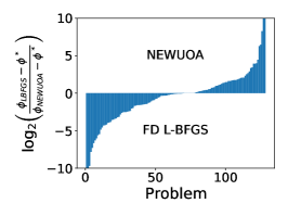
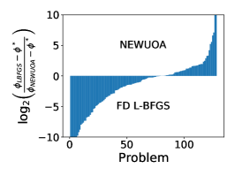
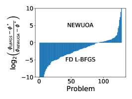
Figure 26: Noisy Case. Log-ratio optimality gap profiles comparing forward difference l-bfgs against newuoa with $p=n+2$ points. The noise levels are $\sigma_{f}=10^{-1}$ (top left), $\sigma_{f}=10^{-3}$ (top right), $10^{-5}$ (bottom left), and $10^{-7}$ (bottom right).

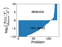
Figure 27: Noisy Case. Log-ratio optimality gap profiles comparing central difference l-bfgs against newuoa with $p=3n+1$ points. The noise levels are $\sigma_{f}=10^{-1}$ (top left), $\sigma_{f}=10^{-3}$ (top right), $10^{-5}$ (bottom left), and $10^{-7}$ (bottom right).

B.2 Trust Region Radius

One can also ask if decreasing the final trust region radius could allow newuoa to converge to a better solution. To test this, we change $\rho_{\text{end}}=10^{-12}$ and compare against the default $\rho_{\text{end}}=10^{-6}$ in Figure 28. From our experiments, changing the final trust region radius makes almost no difference on the solution quality and efficiency.

Figure 28: Noisy Case with $\sigma_{f}=10^{-5}$. Log-ratio optimality gap profiles comparing newuoa with $\rho_{\text{end}}=10^{-6}$ and $10^{-12}$.

Appendix C Complete Numerical Results

In this appendix, we present our complete numerical results.

C.1 Unconstrained Optimization

C.1.1 Noiseless Functions

In this section, we list the number of function evaluations (#feval), ratio between number of function evaluations to the number of function evaluations taken by newuoa (RATIO), CPU time (CPU), and optimality gap ($\phi(x)-\phi^{*}$) for each problem instance in Tables 4-8. Function evaluations marked with a ^∗ denote cases where the algorithm reached the maximum number of function evaluations. Instances where newuoa samples a point that satisfies (2.7) within the initial $2n+1$ evaluations are denoted by ^∗∗. Problems marked with a ^‡ denote cases where newuoa and l-bfgs converge to different minimizers. Optimality gaps marked with a $\dagger$ denote failures of the algorithm to converge to a valid solution satisfying (2.7).

		NEWUOA				FD L-BFGS				CD L-BFGS
Problem	$n$	#feval	RATIO	CPU	$\phi(x)-\phi^{*}$	#feval	RATIO	CPU	$\phi(x)-\phi^{*}$	#feval	RATIO	CPU	$\phi(x)-\phi^{*}$
AIRCRFTB	$5$	$661$	$1.000$	$0.1$	$6.96310-07$	$296$	$0.448$	$0.02$	$6.51810-07$	$536$	$0.811$	$0.03$	$8.28810-07$
ALLINITU	$4$	$41$	$1.000$	$0.09$	$3.07310-06$	$58$	$1.415$	$0.01$	$4.24010-06$	$103$	$2.512$	$0.01$	$4.24010-06$
ARWHEAD	$100$	$201^{**}$	$1.000$	$0.09$	$0.0001000$	$1130$	$5.622$	$0.06$	$2.47410-07$	$2240$	$11.144$	$0.07$	$2.47610-07$
BARD	$3$	$69$	$1.000$	$0.09$	$7.03210-08$	$102$	$1.478$	$0.01$	$5.24410-07$	$176$	$2.551$	$0.01$	$5.24610-07$
BDQRTIC	$100$	$3682$	$1.000$	$1.85$	$3.73110-04$	$3178$	$0.863$	$0.14$	$2.92310-04$	$6308$	$1.713$	$0.18$	$2.91410-04$
BIGGS3	$3$	$73$	$1.000$	$0.09$	$4.59910-07$	$85$	$1.164$	$0.01$	$5.42210-07$	$152$	$2.082$	$0.01$	$5.42310-07$
BIGGS5‡	$5$	$103$	$1.000$	$0.08$	$-3.72210-05$	$416$	$4.039$	$0.04$	$6.65110-07$	$767$	$7.447$	$0.05$	$4.32110-07$
BIGGS6‡	$6$	$338$	$1.000$	$0.08$	$-1.44410-04$	$323$	$0.956$	$0.03$	$5.35710-07$	$593$	$1.754$	$0.03$	$5.65410-07$
BOX2	$2$	$2^{**}$	$1.000$	$0.08$	$5.84710-19$	$57$	$28.500$	$0.01$	$9.94710-07$	$95$	$47.500$	$0.01$	$9.94710-07$
BOX3	$3$	$2^{**}$	$1.000$	$0.08$	$5.84710-19$	$52$	$26.000$	$0.01$	$7.37110-07$	$91$	$45.500$	$0.01$	$7.37110-07$
BRKMCC	$2$	$10$	$1.000$	$0.08$	$1.44010-07$	$32$	$3.200$	$0.0$	$4.06610-09$	$51$	$5.100$	$0.0$	$4.08810-09$
BROWNAL	$10$	$917$	$1.000$	$0.11$	$9.99810-07$	$177$	$0.193$	$0.01$	$1.70710-07$	$331$	$0.361$	$0.01$	$1.70710-07$
BROWNAL	$100$	$18069$	$1.000$	$9.53$	$9.99310-07$	$1039$	$0.058$	$0.07$	$1.04010-07$	$2051$	$0.114$	$0.1$	$1.04710-07$
BROWNAL	$200$	$100000^{*}$	$1.000$	$207.31$	$3.18410-06$	$823$	$0.008$	$0.13$	$8.25410-07$	$1626$	$0.016$	$0.16$	$8.24310-07$
BROWNDEN	$4$	$140$	$1.000$	$0.09$	$2.90010-02$	$131$	$0.936$	$0.01$	$1.44810-02$	$225$	$1.607$	$0.01$	$1.44910-02$
CLIFF	$2$	$84$	$1.000$	$0.09$	$5.22010-07$	$240$	$2.857$	$0.02$	$3.10110-07$	$365$	$4.345$	$0.02$	$2.07610-07$
CRAGGLVY	$4$	$182$	$1.000$	$0.09$	$8.76110-07$	$135$	$0.742$	$0.01$	$5.85410-07$	$244$	$1.341$	$0.01$	$5.85410-07$
CRAGGLVY	$10$	$511$	$1.000$	$0.1$	$1.65010-06$	$482$	$0.943$	$0.03$	$1.17610-06$	$910$	$1.781$	$0.04$	$1.16810-06$
CRAGGLVY	$50$	$2670$	$1.000$	$0.45$	$1.52310-05$	$2301$	$0.862$	$0.1$	$1.28910-05$	$4544$	$1.702$	$0.14$	$1.29210-05$
CRAGGLVY	$100$	$5679$	$1.000$	$2.92$	$3.21910-05$	$4503$	$0.793$	$0.21$	$1.93210-05$	$8946$	$1.575$	$0.29$	$1.93410-05$
CUBE	$2$	$173$	$1.000$	$0.08$	$8.15710-07$	$114$	$0.659$	$0.01$	$3.10710-07$	$190$	$1.098$	$0.01$	$3.03610-07$
DENSCHNA	$2$	$22$	$1.000$	$0.09$	$2.89310-10$	$38$	$1.727$	$0.01$	$9.51710-10$	$64$	$2.909$	$0.01$	$9.52110-10$
DENSCHNB	$2$	$21$	$1.000$	$0.09$	$9.13510-08$	$25$	$1.190$	$0.0$	$3.86710-11$	$42$	$2.000$	$0.0$	$3.87710-11$
DENSCHNC	$2$	$66$	$1.000$	$0.09$	$7.33310-08$	$68$	$1.030$	$0.01$	$8.94910-08$	$111$	$1.682$	$0.01$	$8.95110-08$
DENSCHND	$3$	$312$	$1.000$	$0.07$	$9.79410-07$	$208$	$0.667$	$0.02$	$9.53410-07$	$356$	$1.141$	$0.02$	$9.53710-07$
DENSCHNE	$3$	$127$	$1.000$	$0.09$	$4.48710-07$	$141$	$1.110$	$0.01$	$1.59910-07$	$237$	$1.866$	$0.01$	$1.21010-07$
DENSCHNF	$2$	$28$	$1.000$	$0.09$	$5.07910-09$	$48$	$1.714$	$0.01$	$5.45010-09$	$77$	$2.750$	$0.01$	$5.46810-09$

Table 4: Noiseless Unconstrained CUTEst Problems Tested. $n$ is the number of variables.

		NEWUOA				FD L-BFGS				CD L-BFGS
Problem	$n$	#feval	RATIO	CPU	$\phi(x)-\phi^{*}$	#feval	RATIO	CPU	$\phi(x)-\phi^{*}$	#feval	RATIO	CPU	$\phi(x)-\phi^{*}$
DIXMAANA	$15$	$596$	$1.000$	$0.09$	$9.90910-07$	$138$	$0.232$	$0.01$	$1.09610-07$	$265$	$0.445$	$0.01$	$1.09610-07$
DIXMAANA	$90$	$1594$	$1.000$	$0.61$	$9.62610-07$	$738$	$0.463$	$0.03$	$6.57710-07$	$1465$	$0.919$	$0.04$	$6.57810-07$
DIXMAANA	$300$	$8117$	$1.000$	$37.53$	$9.93610-07$	$2720$	$0.335$	$0.15$	$2.97910-09$	$5428$	$0.669$	$0.21$	$2.97810-09$
DIXMAANB	$15$	$395$	$1.000$	$0.1$	$8.58610-07$	$122$	$0.309$	$0.01$	$3.84510-09$	$233$	$0.590$	$0.01$	$3.84510-09$
DIXMAANB	$90$	$1491$	$1.000$	$0.56$	$9.72410-07$	$647$	$0.434$	$0.03$	$6.53610-10$	$1283$	$0.860$	$0.04$	$6.53710-10$
DIXMAANB	$300$	$6446$	$1.000$	$27.48$	$9.98010-07$	$2117$	$0.328$	$0.15$	$7.82510-10$	$4223$	$0.655$	$0.15$	$7.84510-10$
DIXMAANC	$15$	$197$	$1.000$	$0.08$	$9.74710-07$	$158$	$0.802$	$0.01$	$8.21610-07$	$302$	$1.533$	$0.01$	$8.21610-07$
DIXMAANC	$90$	$1611$	$1.000$	$0.63$	$9.91410-07$	$558$	$0.346$	$0.03$	$1.35210-07$	$1104$	$0.685$	$0.03$	$1.35310-07$
DIXMAANC	$300$	$4643$	$1.000$	$18.87$	$9.96410-07$	$2120$	$0.457$	$0.15$	$5.67410-07$	$4227$	$0.910$	$0.15$	$5.67210-07$
DIXMAAND	$15$	$251$	$1.000$	$0.1$	$9.03610-07$	$179$	$0.713$	$0.01$	$4.53610-07$	$340$	$1.355$	$0.01$	$4.53610-07$
DIXMAAND	$90$	$2090$	$1.000$	$0.81$	$9.55210-07$	$745$	$0.356$	$0.04$	$6.24210-07$	$1474$	$0.705$	$0.04$	$6.24210-07$
DIXMAAND	$300$	$7155$	$1.000$	$33.18$	$9.79110-07$	$2425$	$0.339$	$0.18$	$3.13610-07$	$4834$	$0.676$	$0.18$	$3.13610-07$
DIXMAANE	$15$	$377$	$1.000$	$0.1$	$7.22510-07$	$293$	$0.777$	$0.02$	$4.95810-07$	$564$	$1.496$	$0.02$	$4.95910-07$
DIXMAANE	$90$	$3081$	$1.000$	$1.28$	$9.84010-07$	$3499$	$1.136$	$0.15$	$8.19710-07$	$6956$	$2.258$	$0.2$	$8.20210-07$
DIXMAANE	$300$	$18666$	$1.000$	$107.25$	$9.99310-07$	$19633$	$1.052$	$0.96$	$5.64310-07$	$39197$	$2.100$	$1.42$	$6.03110-07$
DIXMAANF	$15$	$274$	$1.000$	$0.09$	$9.30110-07$	$226$	$0.825$	$0.01$	$7.28510-07$	$434$	$1.584$	$0.01$	$7.28610-07$
DIXMAANF	$90$	$3104$	$1.000$	$1.33$	$9.96410-07$	$2674$	$0.861$	$0.11$	$3.73010-07$	$5313$	$1.712$	$0.15$	$3.73110-07$
DIXMAANF	$300$	$16182$	$1.000$	$92.5$	$9.98810-07$	$14504$	$0.896$	$0.69$	$9.00610-07$	$28952$	$1.789$	$1.06$	$9.01110-07$
DIXMAANG	$15$	$286$	$1.000$	$0.08$	$8.43510-07$	$277$	$0.969$	$0.01$	$2.10110-07$	$533$	$1.864$	$0.02$	$2.10210-07$
DIXMAANG	$90$	$3429$	$1.000$	$1.47$	$9.92210-07$	$2857$	$0.833$	$0.12$	$6.52010-07$	$5678$	$1.656$	$0.16$	$6.52210-07$
DIXMAANG	$300$	$21081$	$1.000$	$126.91$	$9.99910-07$	$14806$	$0.702$	$0.78$	$9.89410-07$	$30158$	$1.431$	$1.1$	$8.87110-07$
DIXMAANH	$15$	$375$	$1.000$	$0.1$	$8.02510-07$	$280$	$0.747$	$0.02$	$1.34110-07$	$537$	$1.432$	$0.02$	$1.34210-07$
DIXMAANH	$90$	$3106$	$1.000$	$1.27$	$9.94310-07$	$2588$	$0.833$	$0.11$	$6.40710-07$	$5138$	$1.654$	$0.15$	$6.40510-07$
DIXMAANH	$300$	$35784$	$1.000$	$212.15$	$9.99910-07$	$14207$	$0.397$	$0.69$	$7.04210-07$	$28356$	$0.792$	$1.05$	$6.75210-07$
DIXMAANI	$15$	$586$	$1.000$	$0.1$	$9.55310-07$	$549$	$0.937$	$0.03$	$9.88010-07$	$1060$	$1.809$	$0.04$	$9.88010-07$
DIXMAANI	$90$	$13092$	$1.000$	$6.05$	$9.96610-07$	$15925$	$1.216$	$0.62$	$9.86210-07$	$33132$	$2.531$	$0.91$	$9.27010-07$
DIXMAANI	$300$	$121834$	$1.000$	$774.33$	$9.99910-07$	$150107^{*}$	$1.232$	$6.82$	$2.11910-06$	$150155^{*}$	$1.232$	$5.3$	$1.72010-05$
DIXMAANJ	$15$	$563$	$1.000$	$0.1$	$9.73610-07$	$479$	$0.851$	$0.03$	$1.80910-07$	$926$	$1.645$	$0.03$	$1.79710-07$
DIXMAANJ	$90$	$12417$	$1.000$	$6.11$	$9.92310-07$	$11508$	$0.927$	$0.53$	$9.62810-07$	$22883$	$1.843$	$0.74$	$9.70610-07$
DIXMAANJ	$300$	$120362$	$1.000$	$718.6$	$9.98710-07$	$77321$	$0.642$	$3.61$	$9.97410-07$	$150156^{*}$	$1.248$	$5.37$	$1.02810-06$
DIXMAANK	$15$	$559$	$1.000$	$0.1$	$9.18110-07$	$533$	$0.953$	$0.03$	$3.24210-07$	$1029$	$1.841$	$0.04$	$3.23010-07$
DIXMAANK	$90$	$12601$	$1.000$	$5.72$	$9.96910-07$	$7463$	$0.592$	$0.3$	$9.90210-07$	$15018$	$1.192$	$0.41$	$9.89310-07$
DIXMAANK	$300$	$80808$	$1.000$	$455.59$	$9.99710-07$	$23567$	$0.292$	$1.12$	$9.62310-07$	$47649$	$0.590$	$1.74$	$9.10810-07$
DIXMAANL	$15$	$752$	$1.000$	$0.1$	$9.74010-07$	$502$	$0.668$	$0.03$	$4.74010-07$	$967$	$1.286$	$0.03$	$4.71410-07$
DIXMAANL	$90$	$10608$	$1.000$	$4.87$	$9.97010-07$	$10323$	$0.973$	$0.41$	$9.51910-07$	$20517$	$1.934$	$0.57$	$8.89110-07$
DIXMAANL	$300$	$150000^{*}$	$1.000$	$875.24$	$3.19210-06$	$34747$	$0.232$	$1.67$	$9.94610-07$	$69364$	$0.462$	$2.51$	$9.92610-07$

Table 5: Noiseless Unconstrained CUTEst Problems Tested. $n$ is the number of variables.

		NEWUOA				FD L-BFGS				CD L-BFGS
Problem	$n$	#feval	RATIO	CPU	$\phi(x)-\phi^{*}$	#feval	RATIO	CPU	$\phi(x)-\phi^{*}$	#feval	RATIO	CPU	$\phi(x)-\phi^{*}$
DQRTIC	$10$	$502$	$1.000$	$0.1$	$9.71910-07$	$258$	$0.514$	$0.02$	$4.43910-07$	$488$	$0.972$	$0.02$	$4.43910-07$
DQRTIC	$50$	$2847$	$1.000$	$0.43$	$8.85210-07$	$1467$	$0.515$	$0.06$	$7.89010-07$	$2894$	$1.017$	$0.08$	$7.88810-07$
DQRTIC	$100$	$6061$	$1.000$	$2.81$	$9.76910-07$	$3277$	$0.541$	$0.13$	$5.47110-07$	$6508$	$1.074$	$0.17$	$5.46210-07$
EDENSCH	$36$	$928$	$1.000$	$0.14$	$2.17510-04$	$577$	$0.622$	$0.03$	$7.34110-05$	$1131$	$1.219$	$0.03$	$7.34110-05$
EIGENALS	$6$	$5^{**}$	$1.000$	$0.08$	$0.0001000$	$83$	$16.600$	$0.01$	$7.34410-09$	$152$	$30.400$	$0.01$	$7.09910-09$
EIGENALS	$110$	$55000^{*}$	$1.000$	$40.44$	$1.71610-03$	$42138$	$0.766$	$2.12$	$9.75810-07$	$55108^{*}$	$1.002$	$2.13$	$2.14210-05$
EIGENBLS‡	$6$	$113$	$1.000$	$0.09$	$-3.03310-04$	$91$	$0.805$	$0.01$	$9.72710-09$	$167$	$1.478$	$0.01$	$9.14510-09$
EIGENBLS	$110$	$37505$	$1.000$	$27.4$	$9.99310-07$	$55010^{*}$	$1.467$	$2.68$	$9.28010-04$	$55088^{*}$	$1.469$	$2.1$	$4.00210-02$
EIGENCLS	$30$	$1630$	$1.000$	$0.19$	$9.38310-07$	$2634$	$1.616$	$0.12$	$9.35310-07$	$5174$	$3.174$	$0.16$	$8.93410-07$
ENGVAL1	$2$	$32$	$1.000$	$0.08$	$6.65110-09$	$38$	$1.188$	$0.0$	$2.19110-07$	$60$	$1.875$	$0.0$	$2.19110-07$
ENGVAL1	$50$	$2234$	$1.000$	$0.38$	$5.21110-05$	$585$	$0.262$	$0.02$	$3.07410-05$	$1148$	$0.514$	$0.03$	$3.07410-05$
ENGVAL1	$100$	$1941$	$1.000$	$0.92$	$1.07610-04$	$1337$	$0.689$	$0.07$	$4.19710-06$	$2651$	$1.366$	$0.07$	$4.19810-06$
EXPFIT	$2$	$42$	$1.000$	$0.09$	$9.58810-07$	$46$	$1.095$	$0.01$	$1.42710-09$	$75$	$1.786$	$0.0$	$1.42010-09$
FLETCBV3‡	$10$	$1106$	$1.000$	$0.11$	$1.06310-03$	$261$	$0.236$	$0.01$	$-1.66410-05$	$521$	$0.471$	$0.02$	$-4.71010-05$
FLETCBV3‡	$100$	$50000^{*}$	$1.000$	$28.66$	$1.3331005$	$19708$	$0.394$	$0.87$	$-3.48610-01$	$16125$	$0.323$	$0.54$	$-1.1071001$
FLETCHBV‡	$10$	$945$	$1.000$	$0.09$	$1.4901005$	$263$	$0.278$	$0.02$	$-1.2781001$	$278$	$0.294$	$0.01$	$-5.3221003$
FLETCHBV‡	$100$	$50000^{*}$	$1.000$	$27.77$	$1.2101013$	$18068$	$0.361$	$0.8$	$-6.2401006$	$20933$	$0.419$	$0.67$	$-7.0161007$
FREUROTH	$2$	$55$	$1.000$	$0.09$	$2.21410-05$	$81$	$1.473$	$0.01$	$3.93210-05$	$134$	$2.436$	$0.01$	$3.93210-05$
FREUROTH	$10$	$367$	$1.000$	$0.09$	$6.52410-04$	$286$	$0.779$	$0.02$	$1.19410-06$	$538$	$1.466$	$0.02$	$1.19410-06$
FREUROTH	$50$	$5840$	$1.000$	$0.86$	$5.84410-03$	$1053$	$0.180$	$0.04$	$4.88810-04$	$2073$	$0.355$	$0.06$	$4.88610-04$
FREUROTH	$100$	$2881$	$1.000$	$1.44$	$1.18810-02$	$1950$	$0.677$	$0.09$	$2.60110-03$	$3868$	$1.343$	$0.12$	$2.58910-03$
GENROSE	$5$	$199$	$1.000$	$0.08$	$9.08610-07$	$226$	$1.136$	$0.02$	$9.52710-09$	$411$	$2.065$	$0.02$	$9.36710-09$
GENROSE	$10$	$645$	$1.000$	$0.1$	$8.36910-07$	$896$	$1.389$	$0.06$	$8.05010-07$	$1614$	$2.502$	$0.06$	$1.03210-07$
GENROSE	$100$	$17249$	$1.000$	$9.45$	$9.95410-07$	$25453$	$1.476$	$1.01$	$8.01310-07$	$50198^{*}$	$2.910$	$1.4$	$1.93910-05$
GULF	$3$	$876$	$1.000$	$0.12$	$6.95410-07$	$225$	$0.257$	$0.03$	$7.91310-08$	$392$	$0.447$	$0.04$	$6.04810-07$
HAIRY	$2$	$261$	$1.000$	$0.09$	$1.21410-06$	$86$	$0.330$	$0.01$	$2.20910-07$	$149$	$0.571$	$0.01$	$2.99610-07$
HELIX	$3$	$65$	$1.000$	$0.09$	$3.56910-08$	$149$	$2.292$	$0.01$	$6.81210-07$	$86$	$1.323$	$0.0$	$8.5211002$†
JENSMP‡	$2$	$4^{**}$	$1.000$	$0.09$	$-5.4691002$	$16$	$4.000$	$0.0$	$0.0001000$	$21$	$5.250$	$0.0$	$0.0001000$
KOWOSB	$4$	$150$	$1.000$	$0.09$	$7.08910-07$	$183$	$1.220$	$0.02$	$2.82410-07$	$332$	$2.213$	$0.02$	$2.82510-07$
MEXHAT	$2$	$46$	$1.000$	$0.09$	$1.03610-02$†	$203$	$4.413$	$0.02$	$7.39510-07$	$339$	$7.370$	$0.02$	$4.70710-07$

Table 6: Noiseless Unconstrained CUTEst Problems Tested. $n$ is the number of variables.

		NEWUOA				FD L-BFGS				CD L-BFGS
Problem	$n$	#feval	RATIO	CPU	$\phi(x)-\phi^{*}$	#feval	RATIO	CPU	$\phi(x)-\phi^{*}$	#feval	RATIO	CPU	$\phi(x)-\phi^{*}$
MOREBV	$10$	$379$	$1.000$	$0.09$	$9.45810-07$	$366$	$0.966$	$0.02$	$6.78210-07$	$695$	$1.834$	$0.03$	$6.84310-07$
MOREBV	$50$	$21488$	$1.000$	$3.71$	$9.98810-07$	$25029^{*}$	$1.165$	$0.98$	$1.36810-06$	$25035^{*}$	$1.165$	$0.68$	$6.08810-06$
MOREBV	$100$	$11143$	$1.000$	$6.29$	$9.99910-07$	$15512$	$1.392$	$0.59$	$9.98510-07$	$31067$	$2.788$	$0.82$	$9.99210-07$
NCB20B	$21$	$478$	$1.000$	$0.11$	$4.09310-05$	$169$	$0.354$	$0.01$	$-4.36810-11$	$322$	$0.674$	$0.01$	$-4.33410-11$
NCB20B	$22$	$627$	$1.000$	$0.11$	$4.36110-05$	$154$	$0.246$	$0.01$	$2.49310-05$	$292$	$0.466$	$0.01$	$2.49310-05$
NCB20B	$50$	$3345$	$1.000$	$0.59$	$9.93610-05$	$1465$	$0.438$	$0.07$	$9.90610-05$	$2892$	$0.865$	$0.1$	$9.91210-05$
NCB20B	$100$	$7309$	$1.000$	$4.02$	$1.96310-04$	$3376$	$0.462$	$0.21$	$1.79410-04$	$6708$	$0.918$	$0.3$	$1.79710-04$
NCB20B	$180$	$11313$	$1.000$	$22.07$	$3.47010-04$	$4375$	$0.387$	$0.35$	$3.38410-04$	$8718$	$0.771$	$0.56$	$3.37910-04$
NONDIA	$10$	$198$	$1.000$	$0.1$	$4.26710-07$	$167$	$0.843$	$0.01$	$1.45910-11$	$298$	$1.505$	$0.01$	$1.05310-11$
NONDIA	$20$	$426$	$1.000$	$0.1$	$8.90310-07$	$341$	$0.800$	$0.02$	$2.57110-10$	$655$	$1.538$	$0.02$	$2.92910-10$
NONDIA	$30$	$569$	$1.000$	$0.12$	$9.93610-07$	$492$	$0.865$	$0.02$	$3.71210-07$	$956$	$1.680$	$0.03$	$3.73810-07$
NONDIA	$50$	$799$	$1.000$	$0.2$	$9.82910-07$	$792$	$0.991$	$0.03$	$3.82510-08$	$1556$	$1.947$	$0.04$	$3.69110-08$
NONDIA	$90$	$1302$	$1.000$	$0.58$	$9.19210-07$	$1301$	$0.999$	$0.06$	$1.23310-07$	$2574$	$1.977$	$0.07$	$1.18810-07$
NONDIA	$100$	$1683$	$1.000$	$0.89$	$9.87310-07$	$1543$	$0.917$	$0.07$	$1.02810-10$	$3057$	$1.816$	$0.09$	$1.12510-10$
NONDQUAR	$100$	$50000^{*}$	$1.000$	$29.28$	$8.67510-06$	$50056^{*}$	$1.001$	$1.88$	$1.13710-05$	$50189^{*}$	$1.004$	$1.32$	$3.61110-05$
OSBORNEA‡	$5$	$1094$	$1.000$	$0.09$	$1.20410-05$	$477$	$0.436$	$0.05$	$8.44210-07$	$888$	$0.812$	$0.06$	$8.39010-07$
OSBORNEB	$11$	$1529$	$1.000$	$0.14$	$9.67810-07$	$1044$	$0.683$	$0.08$	$9.55110-07$	$2216$	$1.449$	$0.11$	$6.31210-07$
PENALTY1	$4$	$577$	$1.000$	$0.09$	$9.99410-07$	$868$	$1.504$	$0.09$	$9.13410-07$	$1425$	$2.470$	$0.09$	$9.85610-07$
PENALTY1	$10$	$1332$	$1.000$	$0.11$	$9.94410-07$	$1523$	$1.143$	$0.09$	$9.90310-07$	$2942$	$2.209$	$0.11$	$8.87310-07$
PENALTY1	$50$	$6082$	$1.000$	$0.89$	$9.98510-07$	$5773$	$0.949$	$0.22$	$9.99410-07$	$11797$	$1.940$	$0.32$	$9.65210-07$
PENALTY1	$100$	$13215$	$1.000$	$6.44$	$9.96910-07$	$11175$	$0.846$	$0.43$	$7.67210-07$	$21381$	$1.618$	$0.57$	$9.91910-07$
PFIT1LS‡	$3$	$417$	$1.000$	$0.11$	$2.89210-04$	$351$	$0.842$	$0.03$	$9.87110-07$	$403$	$0.966$	$0.03$	$6.79510-07$
PFIT2LS‡	$3$	$767$	$1.000$	$0.1$	$1.24310-02$	$1502^{*}$	$1.958$	$0.17$	$2.81810-04$	$1509^{*}$	$1.967$	$0.11$	$1.52810-03$
PFIT3LS‡	$3$	$907$	$1.000$	$0.1$	$8.22810-02$	$1502^{*}$	$1.656$	$0.17$	$1.50410-02$	$1501^{*}$	$1.655$	$0.11$	$3.62210-02$
PFIT4LS‡	$3$	$1088$	$1.000$	$0.1$	$2.67310-01$	$1505^{*}$	$1.383$	$0.15$	$5.42410-02$	$1508^{*}$	$1.386$	$0.1$	$9.18010-02$
QUARTC	$25$	$1004$	$1.000$	$0.13$	$8.88610-07$	$765$	$0.762$	$0.04$	$4.94710-07$	$1492$	$1.486$	$0.05$	$4.94610-07$
QUARTC	$100$	$6061$	$1.000$	$2.82$	$9.76910-07$	$3277$	$0.541$	$0.13$	$5.47110-07$	$6508$	$1.074$	$0.16$	$5.46210-07$
SINEVAL	$2$	$254$	$1.000$	$0.08$	$6.70610-09$	$309$	$1.217$	$0.04$	$3.58510-09$	$522$	$2.055$	$0.04$	$1.30510-07$

Table 7: Noiseless Unconstrained CUTEst Problems Tested. $n$ is the number of variables.

		NEWUOA				FD L-BFGS				CD L-BFGS
Problem	$n$	#feval	RATIO	CPU	$\phi(x)-\phi^{*}$	#feval	RATIO	CPU	$\phi(x)-\phi^{*}$	#feval	RATIO	CPU	$\phi(x)-\phi^{*}$
SINQUAD	$5$	$125$	$1.000$	$0.09$	$6.68210-06$	$61$	$0.488$	$0.01$	$3.06110-06$	$108$	$0.864$	$0.01$	$3.06110-06$
SINQUAD	$50$	$3325$	$1.000$	$0.55$	$1.13210-03$	$795$	$0.239$	$0.04$	$4.48910-06$	$1562$	$0.470$	$0.05$	$4.55310-06$
SINQUAD	$100$	$8318$	$1.000$	$4.3$	$3.98510-03$	$1545$	$0.186$	$0.07$	$2.75510-03$	$3062$	$0.368$	$0.09$	$2.75810-03$
SISSER	$2$	$24$	$1.000$	$0.09$	$8.48910-07$	$54$	$2.250$	$0.01$	$5.87610-07$	$92$	$3.833$	$0.01$	$5.87610-07$
SPARSQUR	$10$	$184$	$1.000$	$0.09$	$8.87610-07$	$184$	$1.000$	$0.01$	$6.33610-07$	$348$	$1.891$	$0.01$	$6.33610-07$
SPARSQUR	$50$	$1645$	$1.000$	$0.29$	$6.77510-07$	$1046$	$0.636$	$0.04$	$3.74410-07$	$2065$	$1.255$	$0.06$	$3.74410-07$
SPARSQUR	$100$	$2932$	$1.000$	$1.37$	$8.99910-07$	$2150$	$0.733$	$0.09$	$3.88010-07$	$4270$	$1.456$	$0.12$	$3.88010-07$
TOINTGSS	$10$	$234$	$1.000$	$0.09$	$1.03810-05$	$24$	$0.103$	$0.0$	$0.0001000$	$45$	$0.192$	$0.0$	$0.0001000$
TOINTGSS	$50$	$775$	$1.000$	$0.18$	$9.72310-06$	$104$	$0.134$	$0.0$	$-3.00010-09$	$205$	$0.265$	$0.01$	$-3.00010-09$
TOINTGSS	$100$	$1199$	$1.000$	$0.55$	$9.77810-06$	$204$	$0.170$	$0.02$	$4.00010-09$	$405$	$0.338$	$0.01$	$4.00010-09$
TQUARTIC	$5$	$92$	$1.000$	$0.09$	$5.44410-07$	$85$	$0.924$	$0.01$	$1.07810-08$	$150$	$1.630$	$0.01$	$1.07410-08$
TQUARTIC	$10$	$277$	$1.000$	$0.09$	$9.84710-07$	$172$	$0.621$	$0.01$	$5.22810-09$	$325$	$1.173$	$0.01$	$5.31310-09$
TQUARTIC	$50$	$5022$	$1.000$	$0.75$	$9.94910-07$	$646$	$0.129$	$0.03$	$1.68110-08$	$1265$	$0.252$	$0.03$	$1.72510-08$
TQUARTIC	$100$	$20515$	$1.000$	$10.51$	$9.99110-07$	$1538$	$0.075$	$0.07$	$6.81810-09$	$3053$	$0.149$	$0.08$	$6.22310-09$
TRIDIA	$10$	$186$	$1.000$	$0.09$	$9.01910-07$	$210$	$1.129$	$0.01$	$5.45110-08$	$396$	$2.129$	$0.01$	$5.44610-08$
TRIDIA	$20$	$446$	$1.000$	$0.1$	$8.06210-07$	$690$	$1.547$	$0.04$	$8.06810-07$	$1340$	$3.004$	$0.04$	$8.06410-07$
TRIDIA	$30$	$768$	$1.000$	$0.13$	$9.96210-07$	$1481$	$1.928$	$0.07$	$6.30910-07$	$2906$	$3.784$	$0.08$	$6.31510-07$
TRIDIA	$50$	$1446$	$1.000$	$0.3$	$8.80610-07$	$3128$	$2.163$	$0.15$	$9.30010-07$	$6187$	$4.279$	$0.19$	$9.29210-07$
TRIDIA	$100$	$3450$	$1.000$	$2.11$	$9.96810-07$	$8783$	$2.546$	$0.32$	$9.67710-07$	$17468$	$5.063$	$0.43$	$9.20810-07$
WATSON	$12$	$4966$	$1.000$	$0.21$	$9.98210-07$	$1324$	$0.267$	$0.08$	$9.77310-07$	$2708$	$0.545$	$0.11$	$9.95010-07$
WATSON	$31$	$15500^{*}$	$1.000$	$1.11$	$6.43810-05$	$13875$	$0.895$	$0.65$	$9.95710-07$	$15530^{*}$	$1.002$	$0.51$	$5.66410-06$
WOODS	$4$	$497$	$1.000$	$0.08$	$1.43410-07$	$178$	$0.358$	$0.02$	$4.44710-09$	$312$	$0.628$	$0.02$	$4.35310-09$
WOODS	$100$	$50000^{*}$	$1.000$	$28.69$	$1.37110-04$	$2972$	$0.059$	$0.13$	$7.20810-07$	$5902$	$0.118$	$0.16$	$6.25210-07$
ZANGWIL2	$2$	$12$	$1.000$	$0.09$	$5.08510-07$	$11$	$0.917$	$0.0$	$-1.00010-10$	$19$	$1.583$	$0.0$	$-9.99910-11$

Table 8: Noiseless Unconstrained CUTEst Problems Tested. $n$ is the number of variables.

C.1.2 Noisy Functions

In this section, we list the best optimality gap ($\phi(x)-\phi^{*}$) and the number of function evaluations (#feval) needed to achieve this for each problem instance, varying the noise level $\sigma_{f}\in\{10^{-1},10^{-3},10^{-5},10^{-7}\}$, in Tables 9-21. Function evaluations marked with a ^∗ denote cases where the algorithm reached the maximum number of function evaluations. Instances where newuoa samples a point that satisfies (2.7) within the initial $2d+1$ evaluations are denoted by ^∗∗. Problems marked with a ^‡ denote cases where newuoa and l-bfgs converge to different minimizers.

			NEWUOA		FD L-BFGS		CD L-BFGS
Problem	$n$	$\sigma_{f}$	#feval	$\phi(x)-\phi^{*}$	#feval	$\phi(x)-\phi^{*}$	#feval	$\phi(x)-\phi^{*}$
AIRCRFTB	$5$	$110-01$	$43$	$7.25710-01$	$53$	$7.27710-01$	$231$	$2.62310-01$
AIRCRFTB	$5$	$110-03$	$70$	$1.77210-01$	$715$	$9.93810-02$	$904$	$6.64810-05$
AIRCRFTB	$5$	$110-05$	$159$	$1.00610-02$	$1221$	$3.35510-04$	$927$	$1.04210-05$
AIRCRFTB	$5$	$110-07$	$317$	$2.89310-04$	$1176$	$4.11910-06$	$1106$	$7.13910-12$
ALLINITU	$4$	$110-01$	$26$	$1.02010-01$	$24$	$2.8811000$	$108$	$1.98010-03$
ALLINITU	$4$	$110-03$	$38$	$9.90110-04$	$97$	$2.61410-04$	$189$	$7.46710-07$
ALLINITU	$4$	$110-05$	$44$	$1.33710-06$	$62$	$1.72110-05$	$320$	$5.60610-09$
ALLINITU	$4$	$110-07$	$58$	$1.18610-08$	$74$	$1.61210-07$	$170$	$3.51810-10$
ARWHEAD	$100$	$110-01$	$201^{**}$	$0.0001000$	$508$	$8.43310-02$	$1022$	$5.89410-02$
ARWHEAD	$100$	$110-03$	$201^{**}$	$0.0001000$	$1035$	$3.52510-02$	$2037$	$1.30510-03$
ARWHEAD	$100$	$110-05$	$201^{**}$	$0.0001000$	$1765$	$1.92510-04$	$2444$	$5.06110-06$
ARWHEAD	$100$	$110-07$	$201^{**}$	$0.0001000$	$1434$	$1.34610-05$	$2660$	$6.84110-09$
BARD	$3$	$110-01$	$20$	$1.66510-01$	$53$	$9.34710-01$	$102$	$2.11910-03$
BARD	$3$	$110-03$	$36$	$5.40310-04$	$77$	$1.03010-03$	$116$	$1.87610-03$
BARD	$3$	$110-05$	$47$	$1.25610-03$	$294$	$1.89810-03$	$310$	$2.73110-06$
BARD	$3$	$110-07$	$87$	$1.68510-07$	$198$	$6.07610-08$	$230$	$3.75310-09$
BDQRTIC	$100$	$110-01$	$2283$	$1.1321000$	$2482$	$5.2461000$	$3476$	$2.69710-01$
BDQRTIC	$100$	$110-03$	$4736$	$9.55410-02$	$2664$	$1.09910-01$	$6583$	$4.06110-03$
BDQRTIC	$100$	$110-05$	$7755$	$4.13410-03$	$6619$	$3.95710-04$	$11431$	$9.21610-07$
BDQRTIC	$100$	$110-07$	$5083$	$6.41910-06$	$6543$	$6.82910-06$	$9934$	$4.42310-09$
BIGGS3‡	$3$	$110-01$	$8$	$1.3661000$	$160$	$1.3111000$	$168$	$9.75610-01$
BIGGS3‡	$3$	$110-03$	$67$	$2.25110-03$	$155$	$6.55610-04$	$389$	$1.95810-05$
BIGGS3‡	$3$	$110-05$	$73$	$1.77610-06$	$78$	$2.85810-06$	$293$	$1.38010-06$
BIGGS3‡	$3$	$110-07$	$85$	$1.15410-08$	$95$	$1.53810-06$	$389$	$8.35710-09$
BIGGS5‡	$5$	$110-01$	$30$	$1.3001000$	$15$	$1.3731000$	$435$	$1.11310-01$
BIGGS5‡	$5$	$110-03$	$113$	$3.93210-02$	$266$	$1.18110-01$	$253$	$3.14210-02$
BIGGS5‡	$5$	$110-05$	$176$	$-4.49610-03$	$285$	$1.80810-02$	$818$	$8.48710-06$
BIGGS‡5	$5$	$110-07$	$265$	$-5.52910-03$	$580$	$6.90510-05$	$1077$	$2.32110-08$
BIGGS6	$6$	$110-01$	$30$	$3.14410-01$	$121$	$3.51510-01$	$283$	$2.85510-01$
BIGGS6	$6$	$110-03$	$43$	$2.93710-01$	$126$	$2.89710-01$	$1549$	$3.09210-02$
BIGGS6	$6$	$110-05$	$363$	$-4.55010-03$	$586$	$-3.40210-03$	$1324$	$-5.56810-03$
BIGGS6	$6$	$110-07$	$657$	$-5.61210-03$	$1612$	$-5.60810-03$	$1778$	$-5.64810-03$
BOX2	$2$	$110-01$	$2^{**}$	$5.84710-19$	$187$	$7.59010-02$	$26$	$3.16810-01$
BOX2	$2$	$110-03$	$2^{**}$	$5.84710-19$	$66$	$4.86110-01$	$387$	$1.27610-06$
BOX2	$2$	$110-05$	$2^{**}$	$5.84710-19$	$42$	$4.08910-06$	$132$	$1.36210-06$
BOX2	$2$	$110-07$	$2^{**}$	$5.84710-19$	$56$	$1.84910-06$	$108$	$2.69310-08$
BOX3	$3$	$110-01$	$2^{**}$	$5.84710-19$	$28$	$2.05610-02$	$55$	$2.10210-02$
BOX3	$3$	$110-03$	$2^{**}$	$5.84710-19$	$181$	$1.40810-03$	$94$	$4.05410-06$
BOX3	$3$	$110-05$	$2^{**}$	$5.84710-19$	$86$	$9.69710-06$	$149$	$6.27310-07$
BOX3	$3$	$110-07$	$2^{**}$	$5.84710-19$	$67$	$6.79110-07$	$370$	$4.09310-08$
BRKMCC	$2$	$110-01$	$14$	$1.16010-02$	$107$	$1.08510-01$	$71$	$4.54210-03$
BRKMCC	$2$	$110-03$	$22$	$8.43410-08$	$55$	$3.64910-04$	$51$	$1.40710-06$
BRKMCC	$2$	$110-05$	$10$	$1.37110-07$	$45$	$5.22110-05$	$62$	$2.56510-10$
BRKMCC	$2$	$110-07$	$19$	$3.32510-10$	$34$	$4.96110-08$	$156$	$1.99510-10$

Table 9: Noisy Unconstrained CUTEst Problems Tested. $n$ is the number of variables. $\sigma_{f}$ is the standard deviation of the noise.

			NEWUOA		FD L-BFGS		CD L-BFGS
Problem	$n$	$\sigma_{f}$	#feval	$\phi(x)-\phi^{*}$	#feval	$\phi(x)-\phi^{*}$	#feval	$\phi(x)-\phi^{*}$
BROWNAL	$10$	$110-01$	$46$	$9.21210-02$	$53$	$2.71910-02$	$384$	$4.20210-05$
BROWNAL	$10$	$110-03$	$123$	$1.23210-02$	$65$	$5.75910-05$	$223$	$2.96910-05$
BROWNAL	$10$	$110-05$	$248$	$3.21810-04$	$77$	$3.06210-05$	$740$	$1.09210-05$
BROWNAL	$10$	$110-07$	$458$	$6.91510-06$	$77$	$2.97410-05$	$821$	$2.97110-05$
BROWNAL	$100$	$110-01$	$610$	$1.1641000$	$725$	$5.05510-02$	$2664$	$1.29710-05$
BROWNAL	$100$	$110-03$	$4084$	$2.87710-02$	$725$	$5.54110-04$	$3677$	$1.28710-05$
BROWNAL	$100$	$110-05$	$7907$	$3.83910-04$	$725$	$1.90810-05$	$3763$	$3.09610-08$
BROWNAL	$100$	$110-07$	$11449$	$7.99910-05$	$827$	$1.33610-05$	$3540$	$2.44510-08$
BROWNAL	$200$	$110-01$	$1514$	$7.94510-01$	$821$	$5.42310-03$	$7494$	$8.71910-07$
BROWNAL	$200$	$110-03$	$11839$	$3.64510-02$	$821$	$4.20510-04$	$7494$	$8.23410-07$
BROWNAL	$200$	$110-05$	$22817$	$3.57410-04$	$1833$	$1.07310-05$	$5291$	$9.19810-09$
BROWNAL	$200$	$110-07$	$26754$	$5.22810-06$	$1833$	$9.28410-07$	$1626$	$8.24310-07$
BROWNDEN	$4$	$110-01$	$219$	$3.76210-02$	$151$	$5.20910-01$	$327$	$1.62310-04$
BROWNDEN	$4$	$110-03$	$163$	$3.18310-04$	$358$	$3.29810-03$	$276$	$5.08310-07$
BROWNDEN	$4$	$110-05$	$239$	$1.42810-06$	$351$	$3.11610-05$	$751$	$2.21210-09$
BROWNDEN	$4$	$110-07$	$224$	$1.02010-08$	$159$	$1.90910-07$	$292$	$-4.07510-10$
CLIFF	$2$	$110-01$	$19$	$9.25210-02$	$51$	$2.9021002$	$809$	$5.15310-01$
CLIFF	$2$	$110-03$	$31$	$1.38910-03$	$201$	$2.9021002$	$412$	$3.19010-04$
CLIFF	$2$	$110-05$	$25$	$8.08910-04$	$644$	$1.0271000$	$272$	$2.20910-04$
CLIFF	$2$	$110-07$	$68$	$1.70510-08$	$407$	$4.05410-02$	$335$	$2.19210-04$
CRAGGLVY	$4$	$110-01$	$14$	$8.94610-01$	$253$	$7.32710-01$	$285$	$4.78210-02$
CRAGGLVY	$4$	$110-03$	$72$	$4.04810-03$	$271$	$7.55110-03$	$147$	$5.39710-04$
CRAGGLVY	$4$	$110-05$	$173$	$1.96010-05$	$262$	$8.39610-05$	$338$	$6.25310-06$
CRAGGLVY	$4$	$110-07$	$199$	$1.18610-06$	$160$	$3.74910-04$	$620$	$3.18810-08$
CRAGGLVY	$10$	$110-01$	$195$	$6.51110-01$	$663$	$3.0231001$	$912$	$2.33610-01$
CRAGGLVY	$10$	$110-03$	$345$	$4.33710-02$	$731$	$2.44410-02$	$828$	$5.64710-04$
CRAGGLVY	$10$	$110-05$	$573$	$7.12010-04$	$716$	$6.67310-04$	$1466$	$4.75110-07$
CRAGGLVY	$10$	$110-07$	$1066$	$7.87410-07$	$1602$	$5.15010-06$	$1466$	$4.12110-09$
CRAGGLVY	$50$	$110-01$	$1364$	$1.9681000$	$2041$	$5.8341000$	$3529$	$8.58510-01$
CRAGGLVY	$50$	$110-03$	$1853$	$4.98910-02$	$4908$	$5.23310-02$	$4192$	$9.90110-03$
CRAGGLVY	$50$	$110-05$	$2312$	$4.36310-04$	$3101$	$9.89810-04$	$5860$	$1.28110-05$
CRAGGLVY	$50$	$110-07$	$3654$	$2.35710-06$	$7127$	$9.97810-06$	$7120$	$4.85610-08$
CRAGGLVY	$100$	$110-01$	$3091$	$2.9741000$	$5275$	$1.2281001$	$7272$	$1.4691000$
CRAGGLVY	$100$	$110-03$	$5041$	$1.87810-01$	$3918$	$6.38610-01$	$7959$	$1.29810-02$
CRAGGLVY	$100$	$110-05$	$4955$	$4.72710-04$	$6241$	$5.72910-03$	$15314$	$1.57310-05$
CRAGGLVY	$100$	$110-07$	$7008$	$5.22310-06$	$11106$	$3.05310-05$	$12688$	$2.63510-07$
CUBE	$2$	$110-01$	$26$	$2.0981000$	$34$	$6.75810-02$	$65$	$4.38010-02$
CUBE	$2$	$110-03$	$68$	$9.52410-02$	$43$	$4.16410-02$	$346$	$7.35010-04$
CUBE	$2$	$110-05$	$135$	$1.07510-03$	$40$	$4.26710-02$	$213$	$2.04910-07$
CUBE	$2$	$110-07$	$145$	$3.61410-06$	$141$	$9.28610-04$	$563$	$8.02310-08$
DENSCHNA	$2$	$110-01$	$12$	$1.80210-01$	$31$	$1.03210-01$	$72$	$7.13910-02$
DENSCHNA	$2$	$110-03$	$18$	$2.99010-05$	$66$	$1.19610-03$	$387$	$1.37510-06$
DENSCHNA	$2$	$110-05$	$22$	$3.33710-07$	$73$	$1.08710-05$	$82$	$6.06210-09$
DENSCHNA	$2$	$110-07$	$22$	$1.23310-10$	$44$	$5.95110-08$	$151$	$1.45310-11$

Table 10: Noisy Unconstrained CUTEst Problems Tested. $n$ is the number of variables. $\sigma_{f}$ is the standard deviation of the noise.

			NEWUOA		FD L-BFGS		CD L-BFGS
Problem	$n$	$\sigma_{f}$	#feval	$\phi(x)-\phi^{*}$	#feval	$\phi(x)-\phi^{*}$	#feval	$\phi(x)-\phi^{*}$
DENSCHNB	$2$	$110-01$	$14$	$2.28210-02$	$23$	$2.36910-01$	$293$	$4.98210-04$
DENSCHNB	$2$	$110-03$	$17$	$1.80710-05$	$40$	$8.80310-04$	$387$	$1.43210-06$
DENSCHNB	$2$	$110-05$	$27$	$2.69310-07$	$61$	$1.01710-06$	$42$	$5.98310-11$
DENSCHNB	$2$	$110-07$	$26$	$7.58210-09$	$32$	$2.19410-08$	$136$	$9.49810-12$
DENSCHNC	$2$	$110-01$	$30$	$-7.75510-02$	$18$	$5.03310-02$	$281$	$3.32310-02$
DENSCHNC	$2$	$110-03$	$62$	$2.78010-05$	$80$	$1.77510-02$	$219$	$2.20810-05$
DENSCHNC	$2$	$110-05$	$55$	$-1.83410-01$	$160$	$6.36210-06$	$387$	$1.05510-08$
DENSCHNC	$2$	$110-07$	$54$	$-1.83410-01$	$218$	$2.20010-06$	$136$	$-1.28510-10$
DENSCHND	$3$	$110-01$	$142$	$3.5711001$	$269$	$3.0301001$	$228$	$1.31810-03$
DENSCHND	$3$	$110-03$	$279$	$2.25810-03$	$216$	$1.2881001$	$414$	$4.83610-05$
DENSCHND	$3$	$110-05$	$216$	$2.90910-04$	$240$	$2.21810-05$	$326$	$7.70210-06$
DENSCHND	$3$	$110-07$	$319$	$1.08410-06$	$432$	$1.31810-07$	$679$	$8.61910-08$
DENSCHNE	$3$	$110-01$	$29$	$1.5701000$	$44$	$1.0031000$	$66$	$1.0381000$
DENSCHNE	$3$	$110-03$	$42$	$1.0031000$	$132$	$9.99410-01$	$138$	$9.99310-01$
DENSCHNE	$3$	$110-05$	$73$	$9.99910-01$	$75$	$9.99310-01$	$389$	$9.99310-01$
DENSCHNE	$3$	$110-07$	$116$	$1.08010-08$	$346$	$9.99310-01$	$295$	$1.65110-10$
DENSCHNF	$2$	$110-01$	$19$	$3.02310-03$	$199$	$1.90910-02$	$100$	$2.34910-03$
DENSCHNF	$2$	$110-03$	$26$	$1.38810-05$	$80$	$2.29910-04$	$100$	$8.04510-06$
DENSCHNF	$2$	$110-05$	$32$	$2.91310-08$	$59$	$6.31410-07$	$77$	$2.84310-08$
DENSCHNF	$2$	$110-07$	$38$	$2.40310-09$	$58$	$8.74010-10$	$136$	$4.04810-11$
DIXMAANA	$15$	$110-01$	$202$	$2.0111000$	$278$	$3.9891000$	$727$	$3.80710-03$
DIXMAANA	$15$	$110-03$	$401$	$1.67110-02$	$426$	$4.11110-03$	$516$	$7.51210-06$
DIXMAANA	$15$	$110-05$	$564$	$5.82610-05$	$291$	$2.04110-05$	$413$	$2.14510-08$
DIXMAANA	$15$	$110-07$	$650$	$7.48210-07$	$170$	$1.28810-06$	$660$	$5.43810-11$
DIXMAANA	$90$	$110-01$	$1357$	$9.08910-01$	$1596$	$1.9351001$	$4121$	$1.33810-02$
DIXMAANA	$90$	$110-03$	$1820$	$1.56410-02$	$6783$	$4.44310-02$	$3657$	$3.09310-05$
DIXMAANA	$90$	$110-05$	$2384$	$2.12310-04$	$3552$	$2.36510-04$	$3657$	$1.30410-07$
DIXMAANA	$90$	$110-07$	$2302$	$1.07210-06$	$2031$	$1.82410-06$	$4663$	$1.69010-10$
DIXMAANA	$300$	$110-01$	$11454$	$2.7721000$	$2091$	$5.7521001$	$13555$	$6.27910-02$
DIXMAANA	$300$	$110-03$	$12409$	$3.37010-02$	$5739$	$4.75010-02$	$7272$	$1.39710-04$
DIXMAANA	$300$	$110-05$	$21687$	$2.40610-04$	$4530$	$6.88010-04$	$17895$	$3.06610-07$
DIXMAANA	$300$	$110-07$	$18612$	$3.40410-06$	$5134$	$6.48510-06$	$7860$	$8.72710-10$
DIXMAANB	$15$	$110-01$	$199$	$1.7961000$	$136$	$2.4021000$	$278$	$6.59510-03$
DIXMAANB	$15$	$110-03$	$384$	$1.56310-02$	$700$	$7.14910-03$	$270$	$1.42410-05$
DIXMAANB	$15$	$110-05$	$389$	$1.64410-05$	$351$	$5.28510-05$	$505$	$1.55210-08$
DIXMAANB	$15$	$110-07$	$373$	$2.09810-07$	$274$	$6.29110-07$	$491$	$5.01810-10$
DIXMAANB	$90$	$110-01$	$1588$	$1.1011000$	$277$	$1.6921001$	$1880$	$2.91010-02$
DIXMAANB	$90$	$110-03$	$1406$	$1.02910-02$	$4163$	$1.21310-02$	$1101$	$5.18610-05$
DIXMAANB	$90$	$110-05$	$1918$	$2.72810-04$	$1568$	$9.44310-05$	$2937$	$2.26310-07$
DIXMAANB	$90$	$110-07$	$1932$	$1.52310-06$	$2282$	$5.62110-07$	$2937$	$1.31810-09$
DIXMAANB	$300$	$110-01$	$7971$	$2.5041000$	$905$	$5.6601001$	$11680$	$5.94710-02$
DIXMAANB	$300$	$110-03$	$12927$	$3.55510-02$	$11239$	$9.52910-02$	$7371$	$2.93510-04$
DIXMAANB	$300$	$110-05$	$14656$	$2.96010-04$	$8463$	$2.76910-03$	$14914$	$1.84910-06$
DIXMAANB	$300$	$110-07$	$19729$	$3.25610-06$	$5138$	$2.71110-05$	$7282$	$1.16510-09$

Table 11: Noisy Unconstrained CUTEst Problems Tested. $n$ is the number of variables. $\sigma_{f}$ is the standard deviation of the noise.

			NEWUOA		FD L-BFGS		CD L-BFGS
Problem	$n$	$\sigma_{f}$	#feval	$\phi(x)-\phi^{*}$	#feval	$\phi(x)-\phi^{*}$	#feval	$\phi(x)-\phi^{*}$
DIXMAANC	$15$	$110-01$	$123$	$3.67810-01$	$696$	$9.41710-01$	$413$	$4.27710-03$
DIXMAANC	$15$	$110-03$	$214$	$1.69410-03$	$784$	$9.65710-03$	$627$	$7.83410-05$
DIXMAANC	$15$	$110-05$	$252$	$1.52310-04$	$621$	$3.65810-05$	$413$	$2.69510-08$
DIXMAANC	$15$	$110-07$	$249$	$2.68110-07$	$528$	$4.15010-08$	$627$	$1.28310-10$
DIXMAANC	$90$	$110-01$	$853$	$1.6781000$	$2077$	$3.6261000$	$2649$	$1.11210-02$
DIXMAANC	$90$	$110-03$	$2546$	$1.88610-02$	$1016$	$6.65710-02$	$1880$	$4.97310-05$
DIXMAANC	$90$	$110-05$	$2245$	$1.95310-04$	$2971$	$4.66210-04$	$1880$	$1.39810-07$
DIXMAANC	$90$	$110-07$	$2873$	$2.16910-06$	$2869$	$9.70710-06$	$5905$	$1.89410-10$
DIXMAANC	$300$	$110-01$	$5706$	$2.6601000$	$908$	$2.9091001$	$12855$	$5.27810-02$
DIXMAANC	$300$	$110-03$	$15396$	$2.20010-02$	$9990$	$1.60110-01$	$13555$	$1.92410-04$
DIXMAANC	$300$	$110-05$	$17952$	$3.24810-04$	$8167$	$2.04010-04$	$9111$	$2.43910-07$
DIXMAANC	$300$	$110-07$	$20832$	$3.23410-06$	$7261$	$1.07010-05$	$6639$	$9.02110-10$
DIXMAAND	$15$	$110-01$	$197$	$2.2091000$	$71$	$2.4641000$	$394$	$1.83410-02$
DIXMAAND	$15$	$110-03$	$189$	$1.56810-03$	$210$	$3.27210-03$	$1730$	$6.88510-06$
DIXMAAND	$15$	$110-05$	$265$	$2.64010-05$	$517$	$1.97210-04$	$660$	$1.42310-07$
DIXMAAND	$15$	$110-07$	$245$	$3.12010-07$	$583$	$1.87610-06$	$1730$	$6.04710-11$
DIXMAAND	$90$	$110-01$	$1468$	$1.5971000$	$647$	$4.4711000$	$1880$	$2.47610-02$
DIXMAAND	$90$	$110-03$	$2428$	$2.42810-02$	$2637$	$6.03410-02$	$3075$	$1.07510-04$
DIXMAAND	$90$	$110-05$	$1511$	$2.15110-04$	$5883$	$2.67210-04$	$2449$	$2.12610-07$
DIXMAAND	$90$	$110-07$	$2339$	$1.63410-06$	$2957$	$1.45510-06$	$3970$	$4.57610-10$
DIXMAAND	$300$	$110-01$	$6087$	$3.2951000$	$1211$	$2.4871001$	$11680$	$6.23210-02$
DIXMAAND	$300$	$110-03$	$28875$	$4.69510-02$	$15937$	$2.86110-02$	$13555$	$2.32410-04$
DIXMAAND	$300$	$110-05$	$36583$	$1.96810-04$	$7259$	$1.23710-03$	$6695$	$8.30110-07$
DIXMAAND	$300$	$110-07$	$31821$	$2.37910-06$	$6958$	$1.15410-05$	$7282$	$1.25110-09$
DIXMAANE	$15$	$110-01$	$117$	$2.6801000$	$228$	$2.5931000$	$516$	$4.75010-02$
DIXMAANE	$15$	$110-03$	$483$	$6.71910-02$	$907$	$2.56710-03$	$759$	$9.72310-05$
DIXMAANE	$15$	$110-05$	$359$	$6.66210-05$	$496$	$4.38910-05$	$875$	$3.66510-08$
DIXMAANE	$15$	$110-07$	$473$	$5.98110-08$	$515$	$4.41310-07$	$1730$	$2.04310-10$
DIXMAANE	$90$	$110-01$	$957$	$2.0771000$	$2228$	$1.0481001$	$5905$	$1.52210-01$
DIXMAANE	$90$	$110-03$	$2231$	$5.29510-02$	$2558$	$5.72410-02$	$7854$	$2.74510-03$
DIXMAANE	$90$	$110-05$	$2422$	$1.04710-03$	$3592$	$1.65810-03$	$14178$	$2.99010-06$
DIXMAANE	$90$	$110-07$	$3565$	$3.46810-06$	$6643$	$5.02010-06$	$9472$	$1.43410-08$
DIXMAANE	$300$	$110-01$	$5797$	$6.4721000$	$5878$	$1.5761001$	$17895$	$5.08210-01$
DIXMAANE	$300$	$110-03$	$39321$	$1.16010-01$	$11096$	$1.21610-01$	$42978$	$5.04010-03$
DIXMAANE	$300$	$110-05$	$35575$	$3.90710-03$	$16015$	$3.57210-03$	$41288$	$6.96010-05$
DIXMAANE	$300$	$110-07$	$29189$	$1.86410-05$	$27787$	$3.54510-05$	$51466$	$5.90510-08$
DIXMAANF	$15$	$110-01$	$186$	$1.2921000$	$133$	$9.30710-01$	$394$	$8.25910-02$
DIXMAANF	$15$	$110-03$	$189$	$1.05110-02$	$409$	$5.64010-03$	$413$	$3.13910-05$
DIXMAANF	$15$	$110-05$	$296$	$2.32910-05$	$574$	$1.10110-04$	$825$	$8.22010-08$
DIXMAANF	$15$	$110-07$	$351$	$2.81110-07$	$546$	$1.18810-06$	$1730$	$1.11610-10$
DIXMAANF	$90$	$110-01$	$1055$	$1.6231000$	$277$	$6.6761000$	$3143$	$7.56710-02$
DIXMAANF	$90$	$110-03$	$1855$	$1.15010-01$	$2279$	$3.25510-02$	$6862$	$1.65610-03$
DIXMAANF	$90$	$110-05$	$3117$	$2.37910-04$	$4615$	$5.64910-04$	$6955$	$1.94110-06$
DIXMAANF	$90$	$110-07$	$6296$	$1.24810-05$	$4327$	$6.37210-06$	$9524$	$6.81010-09$
DIXMAANF	$300$	$110-01$	$4652$	$2.5811000$	$904$	$2.2661001$	$11680$	$1.54910-01$
DIXMAANF	$300$	$110-03$	$10797$	$1.17310-01$	$4840$	$2.15310-01$	$31414$	$5.26610-03$
DIXMAANF	$300$	$110-05$	$41760$	$2.50110-03$	$15493$	$6.55010-03$	$41516$	$2.24810-05$
DIXMAANF	$300$	$110-07$	$17405$	$3.17510-05$	$22658$	$3.59510-05$	$59871$	$2.08710-08$

Table 12: Noisy Unconstrained CUTEst Problems Tested. $n$ is the number of variables. $\sigma_{f}$ is the standard deviation of the noise.

			NEWUOA		FD L-BFGS		CD L-BFGS
Problem	$n$	$\sigma_{f}$	#feval	$\phi(x)-\phi^{*}$	#feval	$\phi(x)-\phi^{*}$	#feval	$\phi(x)-\phi^{*}$
DIXMAANG	$15$	$110-01$	$118$	$1.3011000$	$53$	$8.76010-01$	$1730$	$2.44610-02$
DIXMAANG	$15$	$110-03$	$219$	$3.59010-03$	$532$	$8.83010-03$	$1104$	$4.67910-05$
DIXMAANG	$15$	$110-05$	$259$	$1.62810-05$	$310$	$9.96510-04$	$1730$	$9.83010-08$
DIXMAANG	$15$	$110-07$	$354$	$1.41910-07$	$1235$	$2.10610-06$	$1730$	$3.41010-10$
DIXMAANG	$90$	$110-01$	$1253$	$1.6301000$	$2284$	$1.7521000$	$4496$	$9.06110-02$
DIXMAANG	$90$	$110-03$	$3690$	$9.78510-02$	$2011$	$3.83410-02$	$6194$	$1.98110-03$
DIXMAANG	$90$	$110-05$	$2545$	$3.13610-04$	$2579$	$8.48110-04$	$6124$	$7.69710-06$
DIXMAANG	$90$	$110-07$	$3047$	$8.06010-06$	$7112$	$6.47910-06$	$8861$	$7.24410-09$
DIXMAANG	$300$	$110-01$	$7837$	$3.5091000$	$908$	$1.2591001$	$12260$	$3.42910-01$
DIXMAANG	$300$	$110-03$	$40449$	$1.09610-01$	$9353$	$2.25910-01$	$17101$	$4.56010-03$
DIXMAANG	$300$	$110-05$	$33893$	$3.07010-03$	$8463$	$2.84610-03$	$35863$	$3.04710-05$
DIXMAANG	$300$	$110-07$	$149998$	$4.68010-04$	$21147$	$6.50110-05$	$44939$	$9.86710-08$
DIXMAANH	$15$	$110-01$	$167$	$5.65610-01$	$54$	$9.55710-01$	$394$	$2.59310-02$
DIXMAANH	$15$	$110-03$	$280$	$7.73810-03$	$395$	$4.27510-03$	$705$	$3.52710-05$
DIXMAANH	$15$	$110-05$	$365$	$3.60310-05$	$419$	$6.57810-05$	$825$	$7.65210-08$
DIXMAANH	$15$	$110-07$	$400$	$1.83610-07$	$767$	$2.55510-07$	$830$	$9.05210-10$
DIXMAANH	$90$	$110-01$	$1598$	$2.3751000$	$963$	$1.9971000$	$3163$	$8.80810-02$
DIXMAANH	$90$	$110-03$	$2287$	$1.07010-01$	$3112$	$9.06410-02$	$8780$	$3.02910-03$
DIXMAANH	$90$	$110-05$	$3252$	$2.56510-04$	$5492$	$8.58610-04$	$6194$	$4.42310-06$
DIXMAANH	$90$	$110-07$	$5217$	$3.16910-06$	$4430$	$6.06110-06$	$8780$	$4.29510-09$
DIXMAANH	$300$	$110-01$	$19419$	$5.4921000$	$1211$	$1.2051001$	$6759$	$3.22210-01$
DIXMAANH	$300$	$110-03$	$33582$	$2.67810-01$	$15009$	$1.09310-01$	$17702$	$4.86110-03$
DIXMAANH	$300$	$110-05$	$25154$	$4.09810-03$	$15460$	$4.81210-03$	$40314$	$1.68810-05$
DIXMAANH	$300$	$110-07$	$25753$	$1.92010-05$	$22065$	$2.28910-05$	$41288$	$8.90410-08$
DIXMAANI	$15$	$110-01$	$113$	$5.92610-01$	$1218$	$1.0321000$	$516$	$3.90910-02$
DIXMAANI	$15$	$110-03$	$358$	$6.61510-03$	$504$	$1.79710-02$	$1053$	$2.34510-03$
DIXMAANI	$15$	$110-05$	$467$	$6.10910-04$	$1343$	$3.26110-04$	$1476$	$1.37410-06$
DIXMAANI	$15$	$110-07$	$636$	$6.94610-06$	$792$	$1.30810-06$	$1611$	$4.60310-09$
DIXMAANI	$90$	$110-01$	$951$	$2.1351000$	$3000$	$4.3821000$	$7696$	$2.63310-01$
DIXMAANI	$90$	$110-03$	$1824$	$4.21510-02$	$2824$	$5.24110-02$	$7466$	$5.75710-03$
DIXMAANI	$90$	$110-05$	$3278$	$7.11410-03$	$5618$	$4.74710-03$	$18792$	$1.81610-04$
DIXMAANI	$90$	$110-07$	$10692$	$2.13410-04$	$12783$	$1.28110-04$	$36022$	$5.63210-07$
DIXMAANI	$300$	$110-01$	$7480$	$5.7311000$	$12317$	$1.7491001$	$21554$	$9.40110-01$
DIXMAANI	$300$	$110-03$	$12194$	$1.43110-01$	$10792$	$1.46710-01$	$43977$	$1.44510-02$
DIXMAANI	$300$	$110-05$	$25477$	$9.91710-03$	$34341$	$6.57410-03$	$70880$	$3.51110-04$
DIXMAANI	$300$	$110-07$	$36578$	$1.92810-04$	$74070$	$2.40610-04$	$150151^{*}$	$1.77910-05$
DIXMAANJ	$15$	$110-01$	$156$	$1.78610-01$	$52$	$6.21910-01$	$1124$	$3.54310-02$
DIXMAANJ	$15$	$110-03$	$309$	$2.56710-02$	$584$	$1.55710-02$	$1536$	$7.97910-04$
DIXMAANJ	$15$	$110-05$	$672$	$7.83810-05$	$835$	$2.74810-04$	$1124$	$7.68110-07$
DIXMAANJ	$15$	$110-07$	$685$	$4.62110-07$	$789$	$3.24610-05$	$2031$	$1.80410-08$
DIXMAANJ	$90$	$110-01$	$1141$	$1.1871000$	$277$	$3.6681000$	$1880$	$7.14910-02$
DIXMAANJ	$90$	$110-03$	$2186$	$4.91210-02$	$2853$	$5.44110-02$	$7696$	$2.85810-03$
DIXMAANJ	$90$	$110-05$	$4146$	$3.59110-03$	$3791$	$3.09010-03$	$11399$	$4.24210-05$
DIXMAANJ	$90$	$110-07$	$13470$	$6.30510-04$	$7251$	$3.69210-05$	$29130$	$2.88310-07$
DIXMAANJ	$300$	$110-01$	$4325$	$2.3911000$	$904$	$1.2361001$	$11680$	$1.83410-01$
DIXMAANJ	$300$	$110-03$	$23360$	$1.28510-01$	$8042$	$1.12310-01$	$36345$	$8.11910-03$
DIXMAANJ	$300$	$110-05$	$19573$	$3.53110-03$	$18352$	$5.43710-03$	$41369$	$5.49110-05$
DIXMAANJ	$300$	$110-07$	$31059$	$1.80110-04$	$33637$	$5.06010-05$	$84610$	$2.77710-06$

Table 13: Noisy Unconstrained CUTEst Problems Tested. $n$ is the number of variables. $\sigma_{f}$ is the standard deviation of the noise.

			NEWUOA		FD L-BFGS		CD L-BFGS
Problem	$n$	$\sigma_{f}$	#feval	$\phi(x)-\phi^{*}$	#feval	$\phi(x)-\phi^{*}$	#feval	$\phi(x)-\phi^{*}$
DIXMAANK	$15$	$110-01$	$123$	$2.03610-01$	$70$	$3.31010-01$	$270$	$5.34510-02$
DIXMAANK	$15$	$110-03$	$226$	$4.14810-02$	$1229$	$1.66010-02$	$1024$	$8.73410-04$
DIXMAANK	$15$	$110-05$	$533$	$4.05410-04$	$759$	$7.89410-05$	$1730$	$3.45210-07$
DIXMAANK	$15$	$110-07$	$710$	$1.11110-06$	$724$	$3.21910-07$	$1595$	$4.57810-09$
DIXMAANK	$90$	$110-01$	$962$	$2.1151000$	$961$	$9.53610-01$	$1880$	$3.04910-01$
DIXMAANK	$90$	$110-03$	$1921$	$4.37110-02$	$2718$	$9.44910-02$	$10211$	$3.17810-03$
DIXMAANK	$90$	$110-05$	$3646$	$8.82710-04$	$7155$	$1.23410-03$	$8157$	$3.21710-05$
DIXMAANK	$90$	$110-07$	$6961$	$5.78010-04$	$5158$	$2.20810-05$	$14626$	$1.15210-06$
DIXMAANK	$300$	$110-01$	$4131$	$3.6571000$	$908$	$6.7651000$	$12777$	$4.52810-01$
DIXMAANK	$300$	$110-03$	$30156$	$1.39610-01$	$10483$	$3.12610-01$	$21925$	$3.81310-03$
DIXMAANK	$300$	$110-05$	$17158$	$7.02910-03$	$16876$	$3.55610-03$	$26675$	$6.70810-05$
DIXMAANK	$300$	$110-07$	$52657$	$1.52710-04$	$15408$	$7.81310-05$	$82360$	$6.62710-07$
DIXMAANL	$15$	$110-01$	$152$	$1.4511000$	$88$	$5.24610-01$	$1246$	$5.97210-02$
DIXMAANL	$15$	$110-03$	$370$	$3.86110-02$	$866$	$1.48510-02$	$1694$	$5.90010-04$
DIXMAANL	$15$	$110-05$	$782$	$6.33010-05$	$1050$	$1.02910-04$	$1476$	$1.10310-06$
DIXMAANL	$15$	$110-07$	$873$	$1.15210-06$	$638$	$1.03910-06$	$1730$	$2.06410-08$
DIXMAANL	$90$	$110-01$	$1230$	$1.2241000$	$1363$	$1.2181000$	$2817$	$1.84610-01$
DIXMAANL	$90$	$110-03$	$2191$	$4.68010-02$	$2539$	$1.42910-01$	$5193$	$2.43310-03$
DIXMAANL	$90$	$110-05$	$3048$	$1.13110-03$	$3152$	$2.45510-03$	$8780$	$3.05010-05$
DIXMAANL	$90$	$110-07$	$7705$	$2.88810-04$	$5990$	$1.84810-05$	$32927$	$1.56710-07$
DIXMAANL	$300$	$110-01$	$7660$	$3.6061000$	$1211$	$6.9001000$	$11674$	$1.73910-01$
DIXMAANL	$300$	$110-03$	$33194$	$1.81310-01$	$11079$	$2.76710-01$	$19562$	$4.73310-03$
DIXMAANL	$300$	$110-05$	$149998$	$3.70510-02$	$10571$	$5.17510-03$	$26767$	$4.07510-05$
DIXMAANL	$300$	$110-07$	$61830$	$7.29610-04$	$24171$	$5.36410-05$	$57101$	$1.89110-06$
DQRTIC	$10$	$110-01$	$139$	$1.78610-01$	$927$	$1.44910-01$	$762$	$2.81610-04$
DQRTIC	$10$	$110-03$	$152$	$4.67610-03$	$304$	$6.10910-03$	$749$	$3.77010-05$
DQRTIC	$10$	$110-05$	$429$	$8.02010-05$	$943$	$3.90510-05$	$675$	$8.73310-09$
DQRTIC	$10$	$110-07$	$405$	$3.78210-08$	$676$	$1.67510-06$	$675$	$1.03210-08$
DQRTIC	$50$	$110-01$	$1672$	$7.13210-01$	$1197$	$8.68110-01$	$2857$	$7.95810-02$
DQRTIC	$50$	$110-03$	$1719$	$7.32410-03$	$2008$	$7.82510-03$	$2651$	$3.03810-04$
DQRTIC	$50$	$110-05$	$2369$	$2.60310-05$	$2629$	$1.44510-04$	$3341$	$1.75810-06$
DQRTIC	$50$	$110-07$	$2435$	$1.47310-06$	$2493$	$1.91510-06$	$3341$	$2.99210-08$
DQRTIC	$100$	$110-01$	$4920$	$3.88510-01$	$4766$	$6.4221000$	$7146$	$4.24810-02$
DQRTIC	$100$	$110-03$	$5612$	$9.56910-03$	$4517$	$2.47410-03$	$5960$	$1.80710-04$
DQRTIC	$100$	$110-05$	$6494$	$5.76710-05$	$6534$	$7.94110-04$	$7146$	$2.06010-06$
DQRTIC	$100$	$110-07$	$6913$	$8.63310-07$	$1119$	$1.9061007$	$7344$	$2.04110-08$
EDENSCH	$36$	$110-01$	$873$	$9.72110-01$	$1071$	$1.2231000$	$2104$	$1.29010-01$
EDENSCH	$36$	$110-03$	$1175$	$1.18710-02$	$2031$	$1.11610-02$	$1772$	$3.79510-04$
EDENSCH	$36$	$110-05$	$1166$	$1.00110-04$	$1324$	$5.17610-04$	$1772$	$8.17310-07$
EDENSCH	$36$	$110-07$	$1331$	$1.08310-06$	$1300$	$3.57210-06$	$1824$	$2.41710-09$
EIGENALS	$6$	$110-01$	$5^{**}$	$0.0001000$	$96$	$5.36410-01$	$509$	$2.10810-01$
EIGENALS	$6$	$110-03$	$5^{**}$	$0.0001000$	$82$	$1.04110-02$	$252$	$5.29910-04$
EIGENALS	$6$	$110-05$	$5^{**}$	$0.0001000$	$250$	$4.29810-04$	$152$	$1.28410-07$
EIGENALS	$6$	$110-07$	$5^{**}$	$0.0001000$	$294$	$5.33110-06$	$395$	$1.28910-10$
EIGENALS	$110$	$110-01$	$2393$	$9.0211000$	$3176$	$1.6921001$	$8820$	$1.40410-01$
EIGENALS	$110$	$110-03$	$6471$	$8.08110-01$	$3365$	$2.27510-01$	$5137$	$1.25310-02$
EIGENALS	$110$	$110-05$	$36272$	$2.11410-02$	$6187$	$1.40710-02$	$41789$	$2.31310-04$
EIGENALS	$110$	$110-07$	$54998$	$2.42310-04$	$32572$	$1.41810-04$	$55103^{*}$	$2.47110-05$

Table 14: Noisy Unconstrained CUTEst Problems Tested. $n$ is the number of variables. $\sigma_{f}$ is the standard deviation of the noise.

			NEWUOA		FD L-BFGS		CD L-BFGS
Problem	$n$	$\sigma_{f}$	#feval	$\phi(x)-\phi^{*}$	#feval	$\phi(x)-\phi^{*}$	#feval	$\phi(x)-\phi^{*}$
EIGENBLS‡	$6$	$110-01$	$51$	$1.42110-01$	$32$	$1.0961000$	$252$	$3.98610-03$
EIGENBLS‡	$6$	$110-03$	$109$	$3.84310-02$	$240$	$1.22310-03$	$376$	$4.33610-05$
EIGENBLS‡	$6$	$110-05$	$217$	$-1.84010-01$	$247$	$2.79210-05$	$299$	$1.34010-07$
EIGENBLS‡	$6$	$110-07$	$307$	$-1.84910-01$	$190$	$9.57610-08$	$256$	$5.40410-10$
EIGENBLS	$110$	$110-01$	$705$	$3.3891000$	$1761$	$1.1221001$	$4023$	$1.7071000$
EIGENBLS	$110$	$110-03$	$5295$	$1.4521000$	$2754$	$1.5961000$	$7292$	$1.5521000$
EIGENBLS	$110$	$110-05$	$18185$	$2.70010-02$	$21793$	$2.39810-02$	$55096^{*}$	$5.81410-03$
EIGENBLS	$110$	$110-07$	$30763$	$5.29910-04$	$46722$	$9.95910-04$	$55088^{*}$	$2.59110-02$
EIGENCLS	$30$	$110-01$	$400$	$1.6101000$	$1107$	$1.1851001$	$1812$	$4.23510-01$
EIGENCLS	$30$	$110-03$	$686$	$3.90510-01$	$1546$	$2.77410-02$	$3424$	$1.36010-03$
EIGENCLS	$30$	$110-05$	$1590$	$1.17610-03$	$1935$	$1.01610-03$	$4427$	$1.11610-05$
EIGENCLS	$30$	$110-07$	$2212$	$6.46510-06$	$3159$	$1.26610-05$	$6325$	$3.77010-08$
ENGVAL1	$2$	$110-01$	$22$	$3.60210-02$	$24$	$5.48710-01$	$146$	$1.98710-02$
ENGVAL1	$2$	$110-03$	$30$	$9.03610-05$	$203$	$4.72210-03$	$146$	$2.48010-05$
ENGVAL1	$2$	$110-05$	$33$	$5.98710-08$	$54$	$2.39710-06$	$91$	$2.26510-08$
ENGVAL1	$2$	$110-07$	$36$	$3.36110-09$	$56$	$3.12910-08$	$91$	$1.71310-11$
ENGVAL1	$50$	$110-01$	$1298$	$1.8681000$	$2612$	$6.1471000$	$1160$	$2.13610-01$
ENGVAL1	$50$	$110-03$	$1125$	$2.26810-02$	$634$	$1.85710-02$	$3720$	$2.67810-04$
ENGVAL1	$50$	$110-05$	$2643$	$1.16010-04$	$894$	$5.71310-05$	$1460$	$2.35910-06$
ENGVAL1	$50$	$110-07$	$2802$	$9.12910-07$	$1354$	$1.62810-06$	$2651$	$2.88910-09$
ENGVAL1	$100$	$110-01$	$2362$	$1.5851000$	$3555$	$1.1871001$	$1638$	$3.39710-01$
ENGVAL1	$100$	$110-03$	$3400$	$1.46210-02$	$2805$	$4.52110-02$	$4885$	$8.85010-04$
ENGVAL1	$100$	$110-05$	$3501$	$1.72910-04$	$1334$	$5.31310-04$	$5960$	$2.44510-06$
ENGVAL1	$100$	$110-07$	$3166$	$1.29310-06$	$4913$	$3.87810-06$	$4095$	$6.08810-09$
EXPFIT	$2$	$110-01$	$17$	$3.2071000$	$54$	$4.9541000$	$126$	$4.79410-02$
EXPFIT	$2$	$110-03$	$33$	$3.94610-03$	$58$	$4.29910-03$	$67$	$4.25610-05$
EXPFIT	$2$	$110-05$	$38$	$3.46310-07$	$107$	$2.06410-06$	$260$	$7.46810-10$
EXPFIT	$2$	$110-07$	$49$	$8.77810-10$	$68$	$2.67710-08$	$91$	$5.01910-11$
FLETCBV3‡	$10$	$110-01$	$21^{**}$	$3.22810-02$	$32$	$3.22810-02$	$21$	$3.22810-02$
FLETCBV3‡	$10$	$110-03$	$21^{**}$	$3.22810-02$	$29$	$3.22810-02$	$21$	$3.22810-02$
FLETCBV3‡	$10$	$110-05$	$22$	$3.22810-02$	$27$	$3.22810-02$	$21$	$3.22810-02$
FLETCBV3‡	$10$	$110-07$	$965$	$8.77410-04$	$27$	$3.22810-02$	$403$	$3.22810-02$
FLETCBV3‡	$100$	$110-01$	$202$	$1.7851005$	$2486$	$1.7851005$	$1952$	$1.7851005$
FLETCBV3‡	$100$	$110-03$	$202$	$1.7851005$	$447$	$1.7851005$	$4029$	$1.7851005$
FLETCBV3‡	$100$	$110-05$	$50000^{*}$	$1.3491005$	$11892$	$1.7851005$	$49799$	$2.0281002$
FLETCBV3‡	$100$	$110-07$	$49999$	$5.7611004$	$222$	$1.7851005$	$50010^{*}$	$1.0151001$
FLETCHBV‡	$10$	$110-01$	$863$	$2.2401004$	$639$	$2.6531003$	$1087$	$1.2181004$
FLETCHBV‡	$10$	$110-03$	$1289$	$1.5401005$	$1118$	$8.3891003$	$1356$	$-4.7641003$
FLETCHBV‡	$10$	$110-05$	$790$	$2.2281005$	$708$	$-4.6051003$	$1445$	$-7.5191003$
FLETCHBV‡	$10$	$110-07$	$977$	$8.4611004$	$759$	$7.2331002$	$952$	$4.2361002$
FLETCHBV‡	$100$	$110-01$	$50000^{*}$	$1.5811013$	$40962$	$-7.1871009$	$50076^{*}$	$-6.3871009$
FLETCHBV‡	$100$	$110-03$	$50000^{*}$	$1.7311013$	$50015^{*}$	$-9.1791009$	$50085^{*}$	$-3.0931009$
FLETCHBV‡	$100$	$110-05$	$50000^{*}$	$1.7041013$	$33119$	$-8.6841008$	$50068^{*}$	$-5.7101009$
FLETCHBV‡	$100$	$110-07$	$50000^{*}$	$1.3911013$	$8369$	$7.4251010$	$50080^{*}$	$-5.3081009$

Table 15: Noisy Unconstrained CUTEst Problems Tested. $n$ is the number of variables. $\sigma_{f}$ is the standard deviation of the noise.

			NEWUOA		FD L-BFGS		CD L-BFGS
Problem	$n$	$\sigma_{f}$	#feval	$\phi(x)-\phi^{*}$	#feval	$\phi(x)-\phi^{*}$	#feval	$\phi(x)-\phi^{*}$
FREUROTH	$2$	$110-01$	$38$	$6.30410-02$	$35$	$5.0151001$	$368$	$3.87710-04$
FREUROTH	$2$	$110-03$	$35$	$5.50710-01$	$347$	$1.66010-03$	$141$	$1.49610-05$
FREUROTH	$2$	$110-05$	$70$	$8.65910-07$	$83$	$9.38110-05$	$387$	$3.30210-08$
FREUROTH	$2$	$110-07$	$73$	$4.59410-10$	$138$	$1.11210-06$	$261$	$4.99610-10$
FREUROTH	$10$	$110-01$	$125$	$4.5551001$	$137$	$5.5481001$	$1466$	$8.70810-03$
FREUROTH	$10$	$110-03$	$371$	$3.96410-03$	$467$	$1.34110-01$	$562$	$4.68610-05$
FREUROTH	$10$	$110-05$	$433$	$3.00410-04$	$295$	$1.85710-03$	$842$	$5.75510-08$
FREUROTH	$10$	$110-07$	$435$	$1.51210-06$	$602$	$1.34810-05$	$630$	$-3.20610-10$
FREUROTH	$50$	$110-01$	$1629$	$5.7441001$	$2466$	$5.5031001$	$2651$	$6.73410-02$
FREUROTH	$50$	$110-03$	$6822$	$6.1371000$	$3983$	$3.72310-02$	$2857$	$5.29910-05$
FREUROTH	$50$	$110-05$	$7662$	$1.34010-03$	$5024$	$3.38710-04$	$2487$	$2.10110-07$
FREUROTH	$50$	$110-07$	$6619$	$9.76210-06$	$1257$	$1.45310-06$	$3063$	$5.97510-10$
FREUROTH	$100$	$110-01$	$1868$	$5.7511001$	$920$	$6.6191001$	$8609$	$6.26810-02$
FREUROTH	$100$	$110-03$	$8308$	$9.5771000$	$3192$	$5.43010-02$	$6050$	$1.75210-04$
FREUROTH	$100$	$110-05$	$5029$	$1.82410-03$	$4095$	$2.29010-04$	$5769$	$4.16810-07$
FREUROTH	$100$	$110-07$	$5293$	$7.50510-06$	$6187$	$1.09810-05$	$5907$	$-5.19110-09$
GENROSE	$5$	$110-01$	$35$	$3.8491000$	$68$	$3.2461000$	$180$	$2.7111000$
GENROSE	$5$	$110-03$	$162$	$4.18210-02$	$234$	$2.5661000$	$446$	$9.02310-04$
GENROSE	$5$	$110-05$	$221$	$8.54310-05$	$260$	$2.54810-03$	$413$	$2.27810-07$
GENROSE	$5$	$110-07$	$261$	$9.02310-07$	$317$	$4.47610-05$	$454$	$1.11310-09$
GENROSE	$10$	$110-01$	$84$	$9.2591000$	$221$	$8.9021000$	$805$	$8.8921000$
GENROSE	$10$	$110-03$	$585$	$4.32110-03$	$446$	$8.8161000$	$1564$	$1.86010-04$
GENROSE	$10$	$110-05$	$654$	$3.11410-05$	$1016$	$7.48510-03$	$1935$	$1.02910-06$
GENROSE	$10$	$110-07$	$726$	$7.30310-07$	$964$	$8.88110-05$	$1904$	$5.18110-10$
GENROSE	$100$	$110-01$	$1868$	$1.1891002$	$3231$	$1.3351002$	$7344$	$1.1191002$
GENROSE	$100$	$110-03$	$15359$	$1.0811002$	$2247$	$1.1081002$	$50024^{*}$	$6.5591001$
GENROSE	$100$	$110-05$	$18075$	$6.88510-03$	$29786$	$5.08110-03$	$50009^{*}$	$2.77010-01$
GENROSE	$100$	$110-07$	$18030$	$1.71910-06$	$29847$	$4.74810-05$	$50005^{*}$	$2.19410-02$
GULF	$3$	$110-01$	$26$	$7.0471000$	$41$	$6.6371000$	$389$	$6.6221000$
GULF	$3$	$110-03$	$38$	$7.0321000$	$38$	$6.6221000$	$229$	$4.53410-03$
GULF	$3$	$110-05$	$115$	$6.88210-02$	$267$	$3.64910-03$	$370$	$4.46210-03$
GULF	$3$	$110-07$	$333$	$6.93010-03$	$217$	$4.38110-03$	$688$	$2.46010-07$
HAIRY	$2$	$110-01$	$49$	$3.4711002$	$71$	$2.7211002$	$387$	$1.95010-04$
HAIRY	$2$	$110-03$	$351$	$2.42610-04$	$186$	$8.52210-04$	$413$	$2.32610-08$
HAIRY	$2$	$110-05$	$226$	$1.25610-08$	$175$	$9.40110-07$	$516$	$5.07410-11$
HAIRY	$2$	$110-07$	$252$	$2.33910-08$	$87$	$1.50810-06$	$210$	$4.97410-14$
HELIX	$3$	$110-01$	$26$	$9.61610-02$	$188$	$7.6151000$	$374$	$2.78510-01$
HELIX	$3$	$110-03$	$38$	$1.86510-02$	$314$	$4.1471000$	$23$	$8.5221002$
HELIX	$3$	$110-05$	$72$	$1.82210-06$	$453$	$3.02110-06$	$23$	$8.5211002$
HELIX	$3$	$110-07$	$84$	$4.56710-07$	$167$	$1.17110-04$	$23$	$8.5211002$
JENSMP‡	$2$	$110-01$	$24$	$-1.7861003$	$18$	$0.0001000$	$21$	$0.0001000$
JENSMP‡	$2$	$110-03$	$78$	$-1.8961003$	$18$	$0.0001000$	$21$	$0.0001000$
JENSMP‡	$2$	$110-05$	$87$	$-1.8961003$	$18$	$0.0001000$	$21$	$0.0001000$
JENSMP‡	$2$	$110-07$	$67$	$-1.8961003$	$18$	$0.0001000$	$21$	$0.0001000$
KOWOSB	$4$	$110-01$	$1^{**}$	$5.00610-03$	$72$	$1.38310-03$	$9$	$5.00610-03$
KOWOSB	$4$	$110-03$	$20$	$2.24010-03$	$261$	$3.30510-03$	$104$	$2.43510-04$
KOWOSB	$4$	$110-05$	$44$	$1.24910-04$	$112$	$1.76710-04$	$220$	$6.11810-05$
KOWOSB	$4$	$110-07$	$111$	$2.69410-05$	$1309$	$6.91510-07$	$314$	$5.63810-08$

Table 16: Noisy Unconstrained CUTEst Problems Tested. $n$ is the number of variables. $\sigma_{f}$ is the standard deviation of the noise.

			NEWUOA		FD L-BFGS		CD L-BFGS
Problem	$n$	$\sigma_{f}$	#feval	$\phi(x)-\phi^{*}$	#feval	$\phi(x)-\phi^{*}$	#feval	$\phi(x)-\phi^{*}$
MEXHAT	$2$	$110-01$	$30$	$1.16610-02$	$98$	$4.47710-01$	$146$	$4.23110-01$
MEXHAT	$2$	$110-03$	$43$	$1.10210-02$	$80$	$8.45010-01$	$709$	$4.22710-01$
MEXHAT	$2$	$110-05$	$45$	$1.11010-02$	$203$	$4.17310-01$	$232$	$1.56810-03$
MEXHAT	$2$	$110-07$	$44$	$1.03610-02$	$210$	$4.22610-01$	$660$	$1.38310-04$
MOREBV	$10$	$110-01$	$1^{**}$	$1.59910-02$	$19$	$1.59910-02$	$21$	$1.59910-02$
MOREBV	$10$	$110-03$	$81$	$1.26210-02$	$131$	$1.45110-02$	$937$	$1.50610-03$
MOREBV	$10$	$110-05$	$184$	$2.34510-03$	$433$	$1.84710-03$	$796$	$1.44110-06$
MOREBV	$10$	$110-07$	$386$	$1.28310-07$	$988$	$7.40210-05$	$1003$	$5.67510-09$
MOREBV	$50$	$110-01$	$1^{**}$	$1.32110-03$	$93$	$1.32110-03$	$101$	$1.32110-03$
MOREBV	$50$	$110-03$	$105$	$1.12210-03$	$101$	$1.32110-03$	$828$	$4.20410-04$
MOREBV	$50$	$110-05$	$746$	$3.98110-04$	$997$	$7.84110-04$	$2064$	$2.29010-05$
MOREBV	$50$	$110-07$	$1322$	$3.02110-05$	$1283$	$4.62110-05$	$12825$	$7.62810-06$
MOREBV	$100$	$110-01$	$1^{**}$	$3.63310-04$	$190$	$3.63310-04$	$201$	$3.63310-04$
MOREBV	$100$	$110-03$	$1^{**}$	$3.63310-04$	$201$	$3.63310-04$	$2669$	$1.49510-04$
MOREBV	$100$	$110-05$	$320$	$2.53810-04$	$309$	$3.57110-04$	$3457$	$6.77210-06$
MOREBV	$100$	$110-07$	$3087$	$1.41710-05$	$2809$	$1.54010-05$	$14045$	$1.54610-06$
NCB20B	$21$	$110-01$	$1^{**}$	$3.00010-03$	$22$	$3.00010-03$	$232$	$3.17710-04$
NCB20B	$21$	$110-03$	$113$	$1.44110-05$	$74$	$2.96410-04$	$421$	$6.28710-06$
NCB20B	$21$	$110-05$	$260$	$1.40210-04$	$1332$	$5.74110-06$	$686$	$6.09810-09$
NCB20B	$21$	$110-07$	$708$	$1.22410-05$	$260$	$4.81610-08$	$650$	$-5.57410-11$
NCB20B	$22$	$110-01$	$121$	$5.38410-03$	$23$	$6.00010-03$	$388$	$1.03610-03$
NCB20B	$22$	$110-03$	$121$	$1.81710-03$	$174$	$8.59410-04$	$935$	$8.92110-04$
NCB20B	$22$	$110-05$	$265$	$2.97110-04$	$298$	$1.07510-05$	$578$	$3.82910-06$
NCB20B	$22$	$110-07$	$715$	$2.30710-05$	$345$	$1.16310-07$	$908$	$2.37210-09$
NCB20B	$50$	$110-01$	$212$	$9.19910-02$	$121$	$1.09910-01$	$938$	$1.88310-02$
NCB20B	$50$	$110-03$	$734$	$7.83610-03$	$1513$	$1.29610-03$	$1866$	$3.56510-04$
NCB20B	$50$	$110-05$	$1757$	$4.54910-04$	$838$	$3.96510-04$	$3623$	$9.63010-05$
NCB20B	$50$	$110-07$	$4316$	$6.69610-05$	$2253$	$8.61910-05$	$23370$	$2.28910-06$
NCB20B	$100$	$110-01$	$481$	$3.87110-01$	$1565$	$3.45810-01$	$2938$	$3.87410-02$
NCB20B	$100$	$110-03$	$1748$	$1.44710-02$	$2557$	$2.89510-02$	$5703$	$8.58810-04$
NCB20B	$100$	$110-05$	$5976$	$7.14310-04$	$5154$	$3.92210-04$	$10509$	$8.21810-05$
NCB20B	$100$	$110-07$	$15651$	$4.30110-05$	$6944$	$6.47610-05$	$32343$	$1.54610-05$
NCB20B	$180$	$110-01$	$1664$	$4.70010-01$	$1648$	$1.1841000$	$5833$	$1.77210-01$
NCB20B	$180$	$110-03$	$6604$	$4.26110-02$	$2007$	$5.42010-02$	$12753$	$1.80710-03$
NCB20B	$180$	$110-05$	$12066$	$1.06710-03$	$10462$	$3.29910-04$	$22900$	$2.85610-05$
NCB20B	$180$	$110-07$	$26507$	$2.78910-05$	$11118$	$2.80410-05$	$28345$	$2.44010-05$
NONDIA	$10$	$110-01$	$84$	$4.1981000$	$407$	$6.5471000$	$124$	$6.4871000$
NONDIA	$10$	$110-03$	$144$	$1.40610-03$	$79$	$6.4811000$	$579$	$1.10110-04$
NONDIA	$10$	$110-05$	$168$	$3.50710-05$	$93$	$6.4801000$	$349$	$5.34210-07$
NONDIA	$10$	$110-07$	$195$	$2.69510-07$	$185$	$1.57510-07$	$322$	$4.42910-10$
NONDIA	$20$	$110-01$	$154$	$2.6661000$	$814$	$4.1491000$	$885$	$4.4851000$
NONDIA	$20$	$110-03$	$356$	$2.29210-03$	$140$	$4.4351000$	$744$	$5.56010-04$
NONDIA	$20$	$110-05$	$403$	$3.16310-05$	$382$	$1.70910-03$	$996$	$4.73810-07$
NONDIA	$20$	$110-07$	$468$	$1.39910-06$	$383$	$4.58810-07$	$1933$	$3.74310-09$
NONDIA	$30$	$110-01$	$199$	$1.4971000$	$169$	$3.2861000$	$517$	$3.2711000$
NONDIA	$30$	$110-03$	$566$	$6.81810-03$	$780$	$1.60610-02$	$1319$	$1.82810-03$
NONDIA	$30$	$110-05$	$589$	$1.47510-04$	$689$	$8.89810-04$	$1082$	$5.28510-06$
NONDIA	$30$	$110-07$	$634$	$3.77110-07$	$1319$	$6.49110-07$	$1551$	$4.32610-09$

Table 17: Noisy Unconstrained CUTEst Problems Tested. $n$ is the number of variables. $\sigma_{f}$ is the standard deviation of the noise.

			NEWUOA		FD L-BFGS		CD L-BFGS
Problem	$n$	$\sigma_{f}$	#feval	$\phi(x)-\phi^{*}$	#feval	$\phi(x)-\phi^{*}$	#feval	$\phi(x)-\phi^{*}$
NONDIA	$50$	$110-01$	$317$	$8.66510-01$	$269$	$1.5051000$	$423$	$1.5201000$
NONDIA	$50$	$110-03$	$635$	$8.81410-03$	$375$	$1.4981000$	$1659$	$2.46710-03$
NONDIA	$50$	$110-05$	$851$	$7.10810-05$	$3599$	$4.64010-04$	$1659$	$6.90810-06$
NONDIA	$50$	$110-07$	$1132$	$1.51710-06$	$1731$	$1.97110-05$	$1556$	$1.12710-08$
NONDIA	$90$	$110-01$	$573$	$3.89310-01$	$1087$	$6.15410-01$	$744$	$5.84310-01$
NONDIA	$90$	$110-03$	$1374$	$3.30110-01$	$563$	$5.76610-01$	$2052$	$9.23210-03$
NONDIA	$90$	$110-05$	$1720$	$9.43010-05$	$564$	$5.78110-01$	$3319$	$2.61010-05$
NONDIA	$90$	$110-07$	$1788$	$2.40310-06$	$1306$	$4.18410-06$	$4057$	$5.88810-08$
NONDIA	$100$	$110-01$	$419$	$3.34210-01$	$418$	$4.85010-01$	$824$	$4.93010-01$
NONDIA	$100$	$110-03$	$1610$	$2.08610-01$	$927$	$4.80310-01$	$4544$	$1.81510-02$
NONDIA	$100$	$110-05$	$1907$	$1.47410-04$	$934$	$4.65810-01$	$4975$	$4.31710-05$
NONDIA	$100$	$110-07$	$2235$	$2.09110-06$	$2668$	$5.75610-05$	$4072$	$1.01010-07$
NONDQUAR	$100$	$110-01$	$828$	$5.74410-01$	$1433$	$7.56410-01$	$3532$	$1.00610-01$
NONDQUAR	$100$	$110-03$	$1842$	$1.88910-02$	$5568$	$2.00010-02$	$7272$	$5.24410-03$
NONDQUAR	$100$	$110-05$	$4661$	$1.47510-03$	$8339$	$1.94610-03$	$20194$	$3.39410-04$
NONDQUAR	$100$	$110-07$	$26783$	$1.70010-04$	$21822$	$1.54910-04$	$50037^{*}$	$3.49710-05$
OSBORNEA‡	$5$	$110-01$	$52$	$1.12710-02$	$8$	$8.79010-01$	$170$	$1.48510-01$
OSBORNEA‡	$5$	$110-03$	$64$	$5.24010-02$	$9$	$8.79010-01$	$496$	$7.58910-04$
OSBORNEA‡	$5$	$110-05$	$135$	$3.04010-03$	$260$	$1.90210-03$	$1638$	$2.43210-05$
OSBORNEA‡	$5$	$110-07$	$504$	$4.40410-05$	$677$	$2.25210-05$	$1033$	$2.24710-05$
OSBORNEB	$11$	$110-01$	$89$	$5.19010-01$	$308$	$6.67710-01$	$1031$	$2.97210-01$
OSBORNEB	$11$	$110-03$	$172$	$3.07510-01$	$829$	$3.21910-01$	$1238$	$7.48010-02$
OSBORNEB	$11$	$110-05$	$1052$	$7.96810-03$	$1249$	$2.88210-03$	$2334$	$7.85410-05$
OSBORNEB	$11$	$110-07$	$1708$	$8.19110-06$	$1555$	$6.68110-06$	$2395$	$9.14310-09$
PENALTY1	$4$	$110-01$	$49$	$1.91710-02$	$40$	$8.68610-03$	$100$	$4.98010-03$
PENALTY1	$4$	$110-03$	$87$	$2.83510-05$	$165$	$3.66110-05$	$95$	$4.49810-05$
PENALTY1	$4$	$110-05$	$117$	$3.57310-05$	$55$	$1.74110-04$	$106$	$3.82910-05$
PENALTY1	$4$	$110-07$	$113$	$2.25410-05$	$97$	$3.82010-05$	$140$	$3.82610-05$
PENALTY1	$10$	$110-01$	$358$	$4.73310-01$	$1167$	$5.62710-02$	$284$	$1.32710-03$
PENALTY1	$10$	$110-03$	$178$	$3.56710-05$	$347$	$2.20710-04$	$353$	$9.09610-05$
PENALTY1	$10$	$110-05$	$194$	$2.46310-05$	$335$	$6.07810-05$	$595$	$6.00510-05$
PENALTY1	$10$	$110-07$	$245$	$2.98510-05$	$352$	$5.88210-05$	$477$	$5.96510-05$
PENALTY1	$50$	$110-01$	$2527$	$5.60610-01$	$2274$	$1.4231000$	$2076$	$8.18010-03$
PENALTY1	$50$	$110-03$	$2455$	$6.14010-05$	$2697$	$1.20110-04$	$2281$	$2.99910-04$
PENALTY1	$50$	$110-05$	$2298$	$5.57610-05$	$1786$	$9.92610-05$	$2384$	$1.32210-04$
PENALTY1	$50$	$110-07$	$3919$	$8.20810-06$	$1523$	$8.61610-05$	$16116$	$7.33810-06$
PENALTY1	$100$	$110-01$	$5649$	$8.75810-01$	$6442$	$6.2361000$	$4687$	$8.42810-03$
PENALTY1	$100$	$110-03$	$6701$	$1.01910-04$	$3923$	$1.48910-04$	$5093$	$1.85910-04$
PENALTY1	$100$	$110-05$	$5940$	$9.28710-05$	$4516$	$1.90410-04$	$5907$	$1.87810-04$
PENALTY1	$100$	$110-07$	$10954$	$1.25610-05$	$6607$	$1.67710-04$	$28399$	$5.19110-06$
PFIT1LS‡	$3$	$110-01$	$35$	$4.0341000$	$67$	$9.2811000$	$389$	$5.2461000$
PFIT1LS‡	$3$	$110-03$	$111$	$9.25510-01$	$1415$	$7.0021000$	$447$	$2.28810-04$
PFIT1LS‡	$3$	$110-05$	$325$	$1.15410-02$	$342$	$2.23510-06$	$502$	$2.58110-06$
PFIT1LS‡	$3$	$110-07$	$482$	$2.95510-04$	$258$	$4.49310-05$	$453$	$2.48910-06$
PFIT2LS‡	$3$	$110-01$	$113$	$5.1741001$	$81$	$9.8741001$	$620$	$2.71210-01$
PFIT2LS‡	$3$	$110-03$	$410$	$2.1361000$	$123$	$1.2451002$	$537$	$6.26910-03$
PFIT2LS‡	$3$	$110-05$	$618$	$5.57010-02$	$430$	$4.75710-03$	$537$	$1.77210-03$
PFIT2LS‡	$3$	$110-07$	$706$	$1.25110-02$	$340$	$2.70410-03$	$870$	$1.64810-03$

Table 18: Noisy Unconstrained CUTEst Problems Tested. $n$ is the number of variables. $\sigma_{f}$ is the standard deviation of the noise.

			NEWUOA		FD L-BFGS		CD L-BFGS
Problem	$n$	$\sigma_{f}$	#feval	$\phi(x)-\phi^{*}$	#feval	$\phi(x)-\phi^{*}$	#feval	$\phi(x)-\phi^{*}$
PFIT3LS‡	$3$	$110-01$	$162$	$1.8681002$	$390$	$7.9441001$	$817$	$3.68210-01$
PFIT3LS‡	$3$	$110-03$	$546$	$7.5611000$	$640$	$9.15910-01$	$612$	$3.27610-02$
PFIT3LS‡	$3$	$110-05$	$1012$	$9.38410-02$	$615$	$4.58710-02$	$702$	$3.15410-02$
PFIT3LS‡	$3$	$110-07$	$1012$	$8.22910-02$	$444$	$4.37410-02$	$1504^{*}$	$2.78210-02$
PFIT4LS‡	$3$	$110-01$	$234$	$2.4641002$	$78$	$2.1441003$	$723$	$1.84210-01$
PFIT4LS‡	$3$	$110-03$	$612$	$2.7361001$	$758$	$6.5701000$	$715$	$1.23410-01$
PFIT4LS‡	$3$	$110-05$	$1181$	$8.87110-01$	$471$	$1.67710-01$	$1506^{*}$	$1.43310-01$
PFIT4LS‡	$3$	$110-07$	$1374$	$2.61910-01$	$597$	$1.24910-01$	$1502^{*}$	$1.08610-01$
QUARTC	$25$	$110-01$	$599$	$4.17210-01$	$1716$	$2.0041000$	$1203$	$1.37610-02$
QUARTC	$25$	$110-03$	$759$	$7.39210-03$	$767$	$3.81110-02$	$1496$	$8.96810-05$
QUARTC	$25$	$110-05$	$828$	$6.20110-06$	$1245$	$8.62010-05$	$1750$	$3.50810-07$
QUARTC	$25$	$110-07$	$1040$	$4.13610-07$	$1584$	$1.14810-06$	$2807$	$1.31310-08$
QUARTC	$100$	$110-01$	$4920$	$3.88510-01$	$4766$	$6.4221000$	$7146$	$4.24810-02$
QUARTC	$100$	$110-03$	$5612$	$9.56910-03$	$4517$	$2.47410-03$	$5960$	$1.80710-04$
QUARTC	$100$	$110-05$	$6494$	$5.76710-05$	$6534$	$7.94110-04$	$7146$	$2.06010-06$
QUARTC	$100$	$110-07$	$6913$	$8.63310-07$	$1119$	$1.9061007$	$7344$	$2.04110-08$
SINEVAL	$2$	$110-01$	$12$	$5.2311000$	$4$	$5.5521000$	$108$	$4.6321000$
SINEVAL	$2$	$110-03$	$152$	$9.33910-01$	$194$	$3.5871000$	$700$	$2.08210-04$
SINEVAL	$2$	$110-05$	$226$	$1.68210-05$	$450$	$1.85610-01$	$488$	$1.36010-07$
SINEVAL	$2$	$110-07$	$295$	$1.84110-08$	$425$	$1.95510-05$	$563$	$9.89910-13$
SINQUAD	$5$	$110-01$	$36$	$1.5031000$	$333$	$5.2191000$	$107$	$1.12110-02$
SINQUAD	$5$	$110-03$	$98$	$8.68210-03$	$79$	$6.18610-03$	$121$	$3.32610-05$
SINQUAD	$5$	$110-05$	$140$	$1.60210-05$	$77$	$3.26010-05$	$121$	$9.62010-08$
SINQUAD	$5$	$110-07$	$170$	$1.17710-06$	$135$	$5.82610-09$	$205$	$-3.93810-10$
SINQUAD	$50$	$110-01$	$1724$	$1.7401000$	$742$	$2.2221001$	$3929$	$1.37610-01$
SINQUAD	$50$	$110-03$	$3724$	$3.11910-02$	$1101$	$9.61510-03$	$3616$	$2.54410-04$
SINQUAD	$50$	$110-05$	$4234$	$3.23610-04$	$849$	$2.58910-04$	$2857$	$6.46710-07$
SINQUAD	$50$	$110-07$	$6464$	$1.67010-06$	$1261$	$1.64410-06$	$2083$	$5.44310-09$
SINQUAD	$100$	$110-01$	$4978$	$4.0961000$	$1247$	$1.0481001$	$3062$	$1.02610-01$
SINQUAD	$100$	$110-03$	$7193$	$2.87610-02$	$2470$	$6.29510-02$	$3265$	$2.13210-04$
SINQUAD	$100$	$110-05$	$10426$	$3.20610-04$	$1948$	$9.25710-04$	$3468$	$5.69410-07$
SINQUAD	$100$	$110-07$	$15008$	$2.26310-06$	$2152$	$3.04610-06$	$4079$	$3.92910-09$
SISSER	$2$	$110-01$	$4^{**}$	$3.00010-04$	$20$	$2.32610-02$	$65$	$2.42410-04$
SISSER	$2$	$110-03$	$15$	$1.76410-04$	$139$	$2.82610-05$	$204$	$1.41510-04$
SISSER	$2$	$110-05$	$20$	$2.27010-05$	$44$	$3.73110-05$	$85$	$2.18810-09$
SISSER	$2$	$110-07$	$27$	$1.46710-08$	$71$	$4.27010-07$	$116$	$6.69510-12$
SPARSQUR	$10$	$110-01$	$42$	$2.77910-01$	$104$	$4.30410-02$	$403$	$5.56110-03$
SPARSQUR	$10$	$110-03$	$85$	$2.67510-03$	$212$	$6.28110-03$	$384$	$6.27410-05$
SPARSQUR	$10$	$110-05$	$184$	$4.91510-05$	$740$	$2.77010-05$	$384$	$3.31710-07$
SPARSQUR	$10$	$110-07$	$241$	$1.37710-06$	$398$	$1.38610-07$	$579$	$1.30710-08$
SPARSQUR	$50$	$110-01$	$1070$	$7.98010-01$	$1303$	$6.39710-01$	$1316$	$1.91810-02$
SPARSQUR	$50$	$110-03$	$1034$	$4.91810-03$	$1078$	$1.95210-02$	$3577$	$9.42510-05$
SPARSQUR	$50$	$110-05$	$1472$	$2.31510-05$	$2755$	$4.13510-05$	$2651$	$5.33810-07$
SPARSQUR	$50$	$110-07$	$1847$	$3.80410-07$	$1706$	$5.90310-06$	$2651$	$6.85810-09$
SPARSQUR	$100$	$110-01$	$2912$	$5.98810-01$	$3387$	$1.9531000$	$5960$	$1.10010-02$
SPARSQUR	$100$	$110-03$	$2484$	$4.67210-03$	$2435$	$5.02910-02$	$3677$	$5.41210-05$
SPARSQUR	$100$	$110-05$	$2664$	$7.15110-05$	$5794$	$1.73710-04$	$4292$	$6.55210-06$
SPARSQUR	$100$	$110-07$	$3757$	$3.00210-07$	$4591$	$2.61010-06$	$5960$	$1.08210-08$

Table 19: Noisy Unconstrained CUTEst Problems Tested. $n$ is the number of variables. $\sigma_{f}$ is the standard deviation of the noise.

			NEWUOA		FD L-BFGS		CD L-BFGS
Problem	$n$	$\sigma_{f}$	#feval	$\phi(x)-\phi^{*}$	#feval	$\phi(x)-\phi^{*}$	#feval	$\phi(x)-\phi^{*}$
TOINTGSS	$10$	$110-01$	$65$	$4.85010-01$	$759$	$2.0721000$	$101$	$1.83110-02$
TOINTGSS	$10$	$110-03$	$164$	$1.44810-02$	$301$	$3.30410-02$	$165$	$8.16710-06$
TOINTGSS	$10$	$110-05$	$211$	$2.84510-05$	$124$	$3.62410-04$	$200$	$2.74410-08$
TOINTGSS	$10$	$110-07$	$277$	$2.11310-07$	$124$	$3.53910-06$	$200$	$5.80210-11$
TOINTGSS	$50$	$110-01$	$388$	$1.0331000$	$563$	$1.1831001$	$724$	$6.15510-02$
TOINTGSS	$50$	$110-03$	$878$	$1.27610-02$	$415$	$4.65110-02$	$2132$	$1.55410-05$
TOINTGSS	$50$	$110-05$	$923$	$1.74810-04$	$693$	$1.14010-03$	$724$	$5.40510-08$
TOINTGSS	$50$	$110-07$	$1574$	$1.03010-06$	$693$	$1.13610-05$	$724$	$-2.87710-09$
TOINTGSS	$100$	$110-01$	$1638$	$1.6931000$	$590$	$7.0901000$	$2660$	$6.48310-02$
TOINTGSS	$100$	$110-03$	$1521$	$2.16510-02$	$509$	$7.54510-02$	$1646$	$3.22810-05$
TOINTGSS	$100$	$110-05$	$2692$	$2.38510-04$	$508$	$1.89810-03$	$2526$	$2.62010-08$
TOINTGSS	$100$	$110-07$	$2312$	$3.44210-06$	$508$	$1.89310-05$	$2526$	$4.04610-09$
TQUARTIC	$5$	$110-01$	$22$	$4.61410-01$	$24$	$6.14210-01$	$40$	$4.54010-01$
TQUARTIC	$5$	$110-03$	$63$	$5.64010-03$	$242$	$9.90210-02$	$234$	$5.29010-04$
TQUARTIC	$5$	$110-05$	$107$	$1.15510-05$	$202$	$8.16010-04$	$818$	$1.00410-06$
TQUARTIC	$5$	$110-07$	$137$	$7.04510-08$	$95$	$1.09810-06$	$163$	$9.19210-09$
TQUARTIC	$10$	$110-01$	$44$	$6.15110-01$	$274$	$7.09710-01$	$92$	$5.46410-01$
TQUARTIC	$10$	$110-03$	$174$	$4.40610-02$	$543$	$2.48510-01$	$344$	$5.22310-03$
TQUARTIC	$10$	$110-05$	$277$	$2.54810-05$	$466$	$4.21710-02$	$722$	$7.38910-06$
TQUARTIC	$10$	$110-07$	$388$	$8.69310-07$	$805$	$6.16010-05$	$535$	$4.25610-08$
TQUARTIC	$50$	$110-01$	$191$	$6.73210-01$	$170$	$7.48010-01$	$310$	$7.00210-01$
TQUARTIC	$50$	$110-03$	$1487$	$3.64810-01$	$1155$	$5.61110-01$	$1534$	$6.79610-01$
TQUARTIC	$50$	$110-05$	$3112$	$6.43510-03$	$1441$	$2.12110-02$	$2117$	$1.39010-04$
TQUARTIC	$50$	$110-07$	$5704$	$8.02710-05$	$3736$	$3.33310-04$	$1785$	$3.64910-07$
TQUARTIC	$100$	$110-01$	$226$	$7.23610-01$	$236$	$7.82810-01$	$610$	$7.42310-01$
TQUARTIC	$100$	$110-03$	$1085$	$7.08910-01$	$790$	$7.23210-01$	$3629$	$7.21910-01$
TQUARTIC	$100$	$110-05$	$26574$	$2.45810-02$	$2675$	$1.76510-01$	$4298$	$5.46010-04$
TQUARTIC	$100$	$110-07$	$31937$	$2.80810-04$	$4860$	$4.76110-04$	$5838$	$2.89410-07$
TRIDIA	$10$	$110-01$	$128$	$1.5551000$	$124$	$1.3921000$	$594$	$3.84710-04$
TRIDIA	$10$	$110-03$	$174$	$1.64910-03$	$305$	$2.06510-02$	$495$	$1.42910-06$
TRIDIA	$10$	$110-05$	$176$	$2.35310-05$	$242$	$3.44910-04$	$698$	$4.78610-09$
TRIDIA	$10$	$110-07$	$226$	$1.20510-07$	$279$	$3.03610-06$	$848$	$2.04310-12$
TRIDIA	$20$	$110-01$	$301$	$7.39110-01$	$812$	$1.0721000$	$2309$	$4.78810-04$
TRIDIA	$20$	$110-03$	$312$	$9.50510-03$	$443$	$1.35210-01$	$1432$	$1.03810-06$
TRIDIA	$20$	$110-05$	$396$	$4.89010-05$	$821$	$4.61610-04$	$2029$	$3.47410-09$
TRIDIA	$20$	$110-07$	$500$	$5.28910-07$	$864$	$3.58810-06$	$1992$	$7.66910-12$
TRIDIA	$30$	$110-01$	$454$	$8.86310-01$	$3249$	$7.5661000$	$2694$	$2.36410-03$
TRIDIA	$30$	$110-03$	$599$	$7.42810-03$	$2486$	$6.49410-02$	$2403$	$4.58610-05$
TRIDIA	$30$	$110-05$	$753$	$1.08310-04$	$1254$	$1.15010-03$	$3111$	$7.82010-07$
TRIDIA	$30$	$110-07$	$849$	$7.45510-07$	$2292$	$5.99710-06$	$4598$	$6.84610-11$
TRIDIA	$50$	$110-01$	$670$	$1.6251000$	$1604$	$8.8411000$	$3723$	$1.19010-01$
TRIDIA	$50$	$110-03$	$1124$	$1.61610-02$	$1824$	$2.45210-01$	$6195$	$7.99110-06$
TRIDIA	$50$	$110-05$	$1056$	$4.10110-04$	$3602$	$1.23710-03$	$5985$	$2.19010-06$
TRIDIA	$50$	$110-07$	$1784$	$1.02210-06$	$3450$	$2.57210-05$	$7640$	$1.63410-08$
TRIDIA	$100$	$110-01$	$2183$	$5.2141000$	$4778$	$2.2021001$	$9774$	$1.52410-01$
TRIDIA	$100$	$110-03$	$4301$	$3.58710-02$	$3474$	$6.74610-01$	$15035$	$9.42110-05$
TRIDIA	$100$	$110-05$	$4682$	$4.70510-04$	$10097$	$2.34010-03$	$20327$	$4.89010-07$
TRIDIA	$100$	$110-07$	$3650$	$4.09310-06$	$11716$	$3.46810-05$	$22968$	$8.91810-09$

Table 20: Noisy Unconstrained CUTEst Problems Tested. $n$ is the number of variables. $\sigma_{f}$ is the standard deviation of the noise.

			NEWUOA		FD L-BFGS		CD L-BFGS
Problem	$n$	$\sigma_{f}$	#feval	$\phi(x)-\phi^{*}$	#feval	$\phi(x)-\phi^{*}$	#feval	$\phi(x)-\phi^{*}$
WATSON	$12$	$110-01$	$91$	$1.60210-01$	$260$	$2.74710-01$	$407$	$9.36210-02$
WATSON	$12$	$110-03$	$170$	$7.11210-02$	$752$	$7.26510-03$	$737$	$8.83110-03$
WATSON	$12$	$110-05$	$708$	$6.53110-04$	$1487$	$2.40310-03$	$1470$	$1.80810-04$
WATSON	$12$	$110-07$	$1664$	$2.35510-04$	$1077$	$1.86810-04$	$1559$	$1.36710-05$
WATSON	$31$	$110-01$	$283$	$1.4441000$	$567$	$2.5961000$	$1379$	$2.72710-01$
WATSON	$31$	$110-03$	$982$	$1.55610-01$	$1465$	$1.64810-01$	$4316$	$6.36710-03$
WATSON	$31$	$110-05$	$4133$	$4.93610-03$	$2191$	$1.68210-02$	$3826$	$1.42010-03$
WATSON	$31$	$110-07$	$13951$	$1.46810-04$	$4582$	$8.71510-04$	$8624$	$1.01310-04$
WOODS	$4$	$110-01$	$86$	$8.6551000$	$378$	$5.20010-01$	$391$	$2.49810-01$
WOODS	$4$	$110-03$	$87$	$7.8731000$	$300$	$1.81810-01$	$567$	$1.24810-05$
WOODS	$4$	$110-05$	$432$	$1.68010-05$	$786$	$1.29510-03$	$513$	$6.02310-07$
WOODS	$4$	$110-07$	$515$	$4.00510-07$	$278$	$3.22410-06$	$391$	$6.20410-10$
WOODS	$100$	$110-01$	$8056$	$1.6171002$	$5272$	$4.9801001$	$5925$	$6.4111000$
WOODS	$100$	$110-03$	$27605$	$4.70010-01$	$9371$	$4.58210-01$	$7344$	$1.66610-03$
WOODS	$100$	$110-05$	$35366$	$1.41510-02$	$4207$	$4.45510-03$	$9097$	$9.51010-06$
WOODS	$100$	$110-07$	$50000^{*}$	$6.21610-02$	$4756$	$7.32610-05$	$7528$	$3.72510-07$
ZANGWIL2	$2$	$110-01$	$7$	$1.45510-03$	$14$	$2.78610-02$	$31$	$1.00910-03$
ZANGWIL2	$2$	$110-03$	$17$	$1.57210-05$	$13$	$1.55710-03$	$31$	$1.98710-06$
ZANGWIL2	$2$	$110-05$	$21$	$6.54310-08$	$13$	$1.16410-06$	$516$	$3.65510-09$
ZANGWIL2	$2$	$110-07$	$16$	$3.96410-10$	$13$	$1.16710-08$	$516$	$-9.15010-11$

Table 21: Noisy Unconstrained CUTEst Problems Tested. $n$ is the number of variables. $\sigma_{f}$ is the standard deviation of the noise.

C.2 Nonlinear Least Squares Problems

C.2.1 Noiseless Functions

In this section, we list the number of function evaluations (#feval), CPU time (CPU), and optimality gap ($\phi(x)-\phi^{*}$) for each problem instance in Tables 22. Function evaluations marked with a ^∗ denote cases where the algorithm reached the maximum number of function evaluations.

		LMDER		DFOLS
Problem	$(n,m)$	#feval	$\phi(x)-\phi^{*}$	#feval	$\phi(x)-\phi^{*}$
LINEAR(FR)	$(9,45)$	$21$	$1.42110-14$	$45$	$-1.42110-14$
LINEAR(FR)	$(9,45)$	$21$	$1.27910-13$	$49$	$0.0001000$
LINEAR(R1)	$(7,35)$	$16$	$-3.09910-07$	$61$	$-3.09910-07$
LINEAR(R1)	$(7,35)$	$16$	$-3.09910-07$	$56$	$-3.09910-07$
LINEAR(R10RC)	$(7,35)$	$16$	$1.49310-08$	$56$	$1.49310-08$
LINEAR(R10RC)	$(7,35)$	$16$	$1.49310-08$	$62$	$1.49310-08$
ROSENBR	$(2,2)$	$39$	$0.0001000$	$50$	$3.78810-24$
ROSENBR	$(2,2)$	$17$	$0.0001000$	$14$	$1.49810-20$
HELIX	$(3,3)$	$49$	$3.94110-59$	$44$	$2.53210-28$
HELIX	$(3,3)$	$57$	$5.92110-47$	$80$	$5.47610-20$
POWELLSG	$(4,4)$	$331$	$6.61010-35$	$54$	$1.07410-18$
POWELLSG	$(4,4)$	$346$	$7.10610-35$	$47$	$1.46710-14$
FREUROTH	$(2,2)$	$60$	$3.68810-06$	$122$	$3.67910-06$
FREUROTH	$(2,2)$	$87$	$3.79310-06$	$107$	$3.67910-06$
BARD	$(3,15)$	$21$	$3.06610-10$	$32$	$3.06610-10$
BARD	$(3,15)$	$169$	$1.7421001$	$107$	$1.06610-01$
KOWOSB	$(4,11)$	$99$	$4.42910-12$	$77$	$3.84910-12$
MEYER	$(3,16)$	$456$	$-4.82910-06$	$1500^{*}$	$3.7151004$
WATSON	$(6,31)$	$57$	$5.35910-11$	$81$	$5.35510-11$
WATSON	$(6,31)$	$85$	$5.35710-11$	$105$	$5.35510-11$
WATSON	$(9,31)$	$144$	$1.39310-13$	$409$	$1.46810-13$
WATSON	$(9,31)$	$134$	$1.38210-13$	$499$	$1.45410-13$
WATSON	$(12,31)$	$276$	$1.19810-15$	$340$	$2.21410-09$
WATSON	$(12,31)$	$181$	$3.63610-16$	$1013$	$2.24610-09$
BOX3D	$(3,10)$	$25$	$3.39010-32$	$52$	$1.92110-27$
JENSMP	$(2,10)$	$46$	$-1.76410-05$	$70$	$-1.76410-05$
BROWNDEN	$(4,20)$	$94$	$1.68410-03$	$167$	$1.62610-03$
BROWNDEN	$(4,20)$	$96$	$1.73310-03$	$189$	$1.62610-03$
CHEBYQUAD	$(6,6)$	$59$	$4.43410-32$	$54$	$1.23910-23$
CHEBYQUAD	$(7,7)$	$58$	$6.91510-32$	$49$	$5.12010-29$
CHEBYQUAD	$(8,8)$	$168$	$-2.72510-10$	$258$	$-2.74310-10$
CHEBYQUAD	$(9,9)$	$94$	$4.14310-32$	$87$	$4.53510-28$
CHEBYQUAD	$(10,10)$	$108$	$1.73110-03$	$191$	$-3.03610-10$
CHEBYQUAD	$(11,11)$	$320$	$-4.42810-10$	$352$	$-4.48110-10$
BROWNAL	$(10,10)$	$79$	$2.84010-29$	$52$	$7.67610-19$
OSBORNE1	$(5,33)$	$157$	$-3.02510-12$	$783$	$3.73710-12$
OSBORNE2	$(11,65)$	$101$	$-3.70510-09$	$150$	$-3.70610-09$
OSBORNE2	$(11,65)$	$148$	$1.7501000$	$138$	$1.7501000$
BDQRTIC	$(8,8)$	$508$	$3.75910-06$	$336$	$8.11110-06$
BDQRTIC	$(10,12)$	$662$	$3.15210-06$	$457$	$3.87410-06$
BDQRTIC	$(11,14)$	$1046$	$3.29610-06$	$554$	$2.04610-05$
BDQRTIC	$(12,16)$	$1119$	$-1.26810-06$	$561$	$5.77510-05$

Table 22: Benchmarking Problems Tested. $n$ is the number of variables and $m$ is the dimension of the residual vector.

		LMDER		DFOLS
Problem	$(n,m)$	#feval	$\phi(x)-\phi^{*}$	#feval	$\phi(x)-\phi^{*}$
CUBE	$(5,5)$	$388$	$0.0001000$	$295$	$3.11910-18$
CUBE	$(6,6)$	$1024$	$0.0001000$	$714$	$4.12710-24$
CUBE	$(8,8)$	$4008^{*}$	$2.09010-08$	$4000^{*}$	$4.75310-11$
MANCINO	$(5,5)$	$19$	$4.22410-22$	$25$	$6.17610-20$
MANCINO	$(5,5)$	$25$	$4.68610-22$	$27$	$8.53610-18$
MANCINO	$(8,8)$	$28$	$5.79510-22$	$23$	$3.15210-12$
MANCINO	$(10,10)$	$34$	$8.21810-22$	$25$	$3.06910-11$
MANCINO	$(12,12)$	$53$	$1.32210-22$	$32$	$2.45410-17$
MANCINO	$(12,12)$	$53$	$5.20110-22$	$35$	$2.79810-09$
HEART8LS	$(8,8)$	$37$	$3.40210-30$	$46$	$1.08210-23$
HEART8LS	$(8,8)$	$109$	$3.40210-30$	$2293$	$1.00110-10$

Table 23: Benchmarking Problems Tested. $n$ is the number of variables and $m$ is the dimension of the residual vector.

C.2.2 Noisy Functions

In this section, we list the best optimality gap ($\phi(x)-\phi^{*}$) and the number of function evaluations (#feval) needed to achieve this for each problem instance, varying the noise level $\sigma_{f}\in\{10^{-1},10^{-3},10^{-5},10^{-7}\}$, in Tables 24-27. Function evaluations marked with a ^∗ denote cases where the algorithm reached the maximum number of function evaluations.

			LMDER		DFOLS
Problem	$(n,m)$	$\sigma_{f}$	#feval	$\phi(x)-\phi^{*}$	#feval	$\phi(x)-\phi^{*}$
LINEAR(FR)	$(9,45)$	$110-01$	$65$	$3.5651001$	$70$	$3.6411001$
LINEAR(FR)	$(9,45)$	$110-03$	$126$	$5.00810-02$	$97$	$6.60610-02$
LINEAR(FR)	$(9,45)$	$110-05$	$115$	$5.17010-04$	$81$	$2.88910-05$
LINEAR(FR)	$(9,45)$	$110-07$	$114$	$5.52310-06$	$76$	$2.29610-06$
LINEAR(FR)	$(9,45)$	$110-01$	$229$	$2.8221002$	$77$	$1.1121003$
LINEAR(FR)	$(9,45)$	$110-03$	$115$	$6.08610-02$	$89$	$2.17910-02$
LINEAR(FR)	$(9,45)$	$110-05$	$115$	$5.48210-04$	$78$	$2.30510-04$
LINEAR(FR)	$(9,45)$	$110-07$	$114$	$5.54610-06$	$76$	$2.24010-06$
LINEAR(R1)	$(7,35)$	$110-01$	$69$	$6.47010-02$	$74$	$3.0811000$
LINEAR(R1)	$(7,35)$	$110-03$	$65$	$3.22110-03$	$84$	$1.48210-04$
LINEAR(R1)	$(7,35)$	$110-05$	$70$	$-2.90410-07$	$74$	$-2.96910-07$
LINEAR(R1)	$(7,35)$	$110-07$	$108$	$-3.09910-07$	$73$	$-3.09810-07$
LINEAR(R1)	$(7,35)$	$110-01$	$68$	$6.47110-02$	$78$	$2.1551000$
LINEAR(R1)	$(7,35)$	$110-03$	$118$	$7.43710-05$	$86$	$1.57710-04$
LINEAR(R1)	$(7,35)$	$110-05$	$106$	$-3.04910-07$	$84$	$-2.92610-07$
LINEAR(R1)	$(7,35)$	$110-07$	$103$	$-3.09910-07$	$79$	$-3.09910-07$
LINEAR(R10RC)	$(7,35)$	$110-01$	$63$	$3.66610-01$	$71$	$8.28010-01$
LINEAR(R10RC)	$(7,35)$	$110-03$	$82$	$7.47210-06$	$82$	$2.77110-04$
LINEAR(R10RC)	$(7,35)$	$110-05$	$106$	$2.10110-08$	$75$	$2.97810-08$
LINEAR(R10RC)	$(7,35)$	$110-07$	$72$	$1.49310-08$	$73$	$1.49310-08$
LINEAR(R10RC)	$(7,35)$	$110-01$	$62$	$3.66610-01$	$79$	$9.20910-01$
LINEAR(R10RC)	$(7,35)$	$110-03$	$67$	$1.27210-03$	$89$	$2.25810-04$
LINEAR(R10RC)	$(7,35)$	$110-05$	$106$	$2.10310-08$	$82$	$1.66010-08$
LINEAR(R10RC)	$(7,35)$	$110-07$	$109$	$1.49510-08$	$75$	$1.98510-08$
ROSENBR	$(2,2)$	$110-01$	$44$	$7.60010-02$	$51$	$4.58410-01$
ROSENBR	$(2,2)$	$110-03$	$77$	$3.07810-07$	$50$	$6.04010-08$
ROSENBR	$(2,2)$	$110-05$	$67$	$4.50110-10$	$55$	$1.12210-10$
ROSENBR	$(2,2)$	$110-07$	$65$	$3.66310-14$	$49$	$2.14810-14$
ROSENBR	$(2,2)$	$110-01$	$105$	$4.11810-03$	$71$	$3.57810-02$
ROSENBR	$(2,2)$	$110-03$	$49$	$7.17710-07$	$35$	$6.09710-11$
ROSENBR	$(2,2)$	$110-05$	$44$	$4.53910-10$	$54$	$3.36510-10$
ROSENBR	$(2,2)$	$110-07$	$29$	$3.06410-14$	$28$	$2.19110-15$
HELIX	$(3,3)$	$110-01$	$61$	$4.15810-02$	$59$	$5.02310-02$
HELIX	$(3,3)$	$110-03$	$61$	$1.32810-06$	$62$	$1.26510-05$
HELIX	$(3,3)$	$110-05$	$71$	$7.01210-10$	$66$	$7.64610-10$
HELIX	$(3,3)$	$110-07$	$70$	$4.89310-14$	$77$	$2.03110-14$
HELIX	$(3,3)$	$110-01$	$61$	$1.7671000$	$66$	$8.70110-03$
HELIX	$(3,3)$	$110-03$	$75$	$5.70710-06$	$76$	$1.42910-06$
HELIX	$(3,3)$	$110-05$	$73$	$4.86510-10$	$74$	$8.03210-10$
HELIX	$(3,3)$	$110-07$	$70$	$5.01610-14$	$47$	$3.08510-16$
POWELLSG	$(4,4)$	$110-01$	$78$	$6.28610-02$	$62$	$9.43610-02$
POWELLSG	$(4,4)$	$110-03$	$82$	$3.49510-06$	$54$	$7.64110-05$
POWELLSG	$(4,4)$	$110-05$	$86$	$3.36410-09$	$54$	$7.25510-10$
POWELLSG	$(4,4)$	$110-07$	$131$	$2.80310-14$	$55$	$4.17410-15$
POWELLSG	$(4,4)$	$110-01$	$79$	$6.33810-02$	$59$	$2.03610-03$
POWELLSG	$(4,4)$	$110-03$	$86$	$3.40410-05$	$64$	$2.12610-07$
POWELLSG	$(4,4)$	$110-05$	$131$	$2.60710-10$	$61$	$1.50210-08$
POWELLSG	$(4,4)$	$110-07$	$121$	$1.69410-13$	$56$	$2.86110-15$

Table 24: Benchmarking Problems Tested. $n$ is the number of variables and $m$ is the dimension of the residual vector.

			LMDER		DFOLS
Problem	$(n,m)$	$\sigma_{f}$	#feval	$\phi(x)-\phi^{*}$	#feval	$\phi(x)-\phi^{*}$
FREUROTH	$(2,2)$	$110-01$	$42$	$1.7241000$	$68$	$4.63410-02$
FREUROTH	$(2,2)$	$110-03$	$48$	$7.58210-03$	$75$	$4.55510-06$
FREUROTH	$(2,2)$	$110-05$	$59$	$7.70410-05$	$113$	$3.71710-06$
FREUROTH	$(2,2)$	$110-07$	$64$	$4.52310-06$	$91$	$3.67910-06$
FREUROTH	$(2,2)$	$110-01$	$55$	$2.5461000$	$83$	$1.31010-02$
FREUROTH	$(2,2)$	$110-03$	$66$	$1.26510-02$	$78$	$1.33110-05$
FREUROTH	$(2,2)$	$110-05$	$80$	$4.98710-05$	$102$	$3.68110-06$
FREUROTH	$(2,2)$	$110-07$	$91$	$7.02710-06$	$122$	$3.67910-06$
BARD	$(3,15)$	$110-01$	$45$	$2.37010-01$	$46$	$5.98710-02$
BARD	$(3,15)$	$110-03$	$41$	$1.16810-05$	$38$	$4.67310-05$
BARD	$(3,15)$	$110-05$	$53$	$4.71310-08$	$34$	$1.40410-09$
BARD	$(3,15)$	$110-07$	$44$	$8.43610-10$	$35$	$3.06810-10$
BARD	$(3,15)$	$110-01$	$41$	$1.3551001$	$56$	$9.25610-02$
BARD	$(3,15)$	$110-03$	$73$	$2.0351001$	$65$	$4.98210-05$
BARD	$(3,15)$	$110-05$	$98$	$2.2821000$	$54$	$1.11410-09$
BARD	$(3,15)$	$110-07$	$115$	$1.6111001$	$102$	$1.06610-01$
KOWOSB	$(4,11)$	$110-01$	$35$	$5.00510-03$	$42$	$3.08810-02$
KOWOSB	$(4,11)$	$110-03$	$57$	$1.41810-04$	$44$	$1.56110-04$
KOWOSB	$(4,11)$	$110-05$	$92$	$4.08110-08$	$60$	$4.91610-08$
KOWOSB	$(4,11)$	$110-07$	$84$	$1.30210-08$	$64$	$2.98110-10$
MEYER	$(3,16)$	$110-01$	$182$	$8.3011004$	$67$	$1.1131005$
MEYER	$(3,16)$	$110-03$	$666$	$4.7701000$	$252$	$7.3801004$
MEYER	$(3,16)$	$110-05$	$504$	$8.42310-03$	$1498$	$4.0221004$
MEYER	$(3,16)$	$110-07$	$497$	$-1.30010-06$	$1500^{*}$	$4.0311004$
WATSON	$(6,31)$	$110-01$	$96$	$1.59210-01$	$71$	$1.23210-01$
WATSON	$(6,31)$	$110-03$	$83$	$1.81810-04$	$79$	$1.32810-04$
WATSON	$(6,31)$	$110-05$	$82$	$6.90510-05$	$82$	$7.37510-07$
WATSON	$(6,31)$	$110-07$	$103$	$5.33310-09$	$78$	$8.70310-10$
WATSON	$(6,31)$	$110-01$	$95$	$2.56210-01$	$80$	$1.15010-01$
WATSON	$(6,31)$	$110-03$	$236$	$4.26710-04$	$82$	$2.05210-04$
WATSON	$(6,31)$	$110-05$	$116$	$5.31110-05$	$87$	$1.67610-07$
WATSON	$(6,31)$	$110-07$	$116$	$2.19710-08$	$85$	$6.03910-10$
WATSON	$(9,31)$	$110-01$	$95$	$1.79110-01$	$95$	$6.32610-02$
WATSON	$(9,31)$	$110-03$	$183$	$2.76110-04$	$113$	$1.11210-04$
WATSON	$(9,31)$	$110-05$	$386$	$3.60310-05$	$114$	$5.71710-06$
WATSON	$(9,31)$	$110-07$	$531$	$1.17510-07$	$220$	$9.38410-10$
WATSON	$(9,31)$	$110-01$	$134$	$1.3381000$	$128$	$3.40610-02$
WATSON	$(9,31)$	$110-03$	$390$	$7.29310-03$	$115$	$2.54310-04$
WATSON	$(9,31)$	$110-05$	$580$	$1.43610-04$	$113$	$4.06110-06$
WATSON	$(9,31)$	$110-07$	$533$	$4.14710-07$	$337$	$5.46410-09$
WATSON	$(12,31)$	$110-01$	$147$	$1.82910-01$	$133$	$4.51810-01$
WATSON	$(12,31)$	$110-03$	$199$	$1.94210-04$	$129$	$4.43110-04$
WATSON	$(12,31)$	$110-05$	$736$	$1.86310-05$	$130$	$1.20210-07$
WATSON	$(12,31)$	$110-07$	$713$	$4.16410-08$	$234$	$1.33710-08$
WATSON	$(12,31)$	$110-01$	$188$	$7.23010-01$	$127$	$1.60010-01$
WATSON	$(12,31)$	$110-03$	$255$	$1.08610-02$	$139$	$2.80210-04$
WATSON	$(12,31)$	$110-05$	$530$	$3.23710-02$	$196$	$1.91110-08$
WATSON	$(12,31)$	$110-07$	$851$	$1.85410-04$	$183$	$1.56010-08$

Table 25: Benchmarking Problems Tested. $n$ is the number of variables and $m$ is the dimension of the residual vector.

			LMDER		DFOLS
Problem	$(n,m)$	$\sigma_{f}$	#feval	$\phi(x)-\phi^{*}$	#feval	$\phi(x)-\phi^{*}$
BOX3D	$(3,10)$	$110-01$	$44$	$1.67410-01$	$53$	$1.18110-01$
BOX3D	$(3,10)$	$110-03$	$63$	$1.53210-03$	$43$	$5.39410-06$
BOX3D	$(3,10)$	$110-05$	$56$	$1.73810-09$	$46$	$5.81810-12$
BOX3D	$(3,10)$	$110-07$	$55$	$1.75810-13$	$57$	$2.24810-13$
JENSMP	$(2,10)$	$110-01$	$46$	$3.7281003$	$47$	$2.68410-01$
JENSMP	$(2,10)$	$110-03$	$44$	$4.10210-02$	$51$	$1.66010-02$
JENSMP	$(2,10)$	$110-05$	$53$	$1.44510-03$	$59$	$6.41510-05$
JENSMP	$(2,10)$	$110-07$	$51$	$-7.21510-06$	$47$	$-8.72010-06$
BROWNDEN	$(4,20)$	$110-01$	$75$	$1.5211003$	$84$	$3.9221002$
BROWNDEN	$(4,20)$	$110-03$	$86$	$3.2771001$	$97$	$2.8971000$
BROWNDEN	$(4,20)$	$110-05$	$98$	$7.49810-02$	$140$	$9.53410-03$
BROWNDEN	$(4,20)$	$110-07$	$105$	$2.52910-03$	$144$	$4.05610-03$
BROWNDEN	$(4,20)$	$110-01$	$90$	$2.3841003$	$102$	$8.0071002$
BROWNDEN	$(4,20)$	$110-03$	$102$	$4.4931001$	$97$	$3.7321000$
BROWNDEN	$(4,20)$	$110-05$	$117$	$4.91210-02$	$115$	$1.44010-01$
BROWNDEN	$(4,20)$	$110-07$	$114$	$2.74310-03$	$130$	$2.79810-03$
CHEBYQUAD	$(6,6)$	$110-01$	$54$	$4.24310-02$	$64$	$2.30410-02$
CHEBYQUAD	$(6,6)$	$110-03$	$57$	$3.02010-02$	$73$	$9.16110-07$
CHEBYQUAD	$(6,6)$	$110-05$	$93$	$4.32210-10$	$61$	$1.44710-11$
CHEBYQUAD	$(6,6)$	$110-07$	$91$	$4.78510-14$	$63$	$1.79210-13$
CHEBYQUAD	$(7,7)$	$110-01$	$46$	$3.37710-02$	$67$	$1.04510-02$
CHEBYQUAD	$(7,7)$	$110-03$	$118$	$6.18210-06$	$64$	$1.90110-05$
CHEBYQUAD	$(7,7)$	$110-05$	$97$	$9.56610-10$	$73$	$2.03010-10$
CHEBYQUAD	$(7,7)$	$110-07$	$95$	$1.04310-13$	$73$	$6.45610-14$
CHEBYQUAD	$(8,8)$	$110-01$	$69$	$2.68310-02$	$79$	$6.16410-02$
CHEBYQUAD	$(8,8)$	$110-03$	$93$	$1.26110-02$	$96$	$1.18210-03$
CHEBYQUAD	$(8,8)$	$110-05$	$128$	$1.03910-03$	$199$	$6.12010-07$
CHEBYQUAD	$(8,8)$	$110-07$	$240$	$6.14710-07$	$208$	$1.28810-09$
CHEBYQUAD	$(9,9)$	$110-01$	$54^{**}$	$2.88810-02$	$86$	$2.59710-02$
CHEBYQUAD	$(9,9)$	$110-03$	$100$	$2.01310-02$	$100$	$4.98110-05$
CHEBYQUAD	$(9,9)$	$110-05$	$134$	$2.32610-09$	$102$	$6.62910-10$
CHEBYQUAD	$(9,9)$	$110-07$	$161$	$3.85610-14$	$104$	$3.01210-14$
CHEBYQUAD	$(10,10)$	$110-01$	$94$	$4.02610-02$	$89$	$2.09110-02$
CHEBYQUAD	$(10,10)$	$110-03$	$153$	$9.23710-04$	$87$	$4.59610-03$
CHEBYQUAD	$(10,10)$	$110-05$	$163$	$5.11410-06$	$113$	$4.62210-05$
CHEBYQUAD	$(10,10)$	$110-07$	$207$	$1.73210-03$	$163$	$5.15110-08$
CHEBYQUAD	$(11,11)$	$110-01$	$78$	$2.98310-02$	$87$	$1.92010-02$
CHEBYQUAD	$(11,11)$	$110-03$	$104$	$9.22510-03$	$93$	$6.27310-03$
CHEBYQUAD	$(11,11)$	$110-05$	$213$	$4.20510-04$	$235$	$8.67010-07$
CHEBYQUAD	$(11,11)$	$110-07$	$449$	$1.14110-06$	$246$	$1.47310-08$

Table 26: Benchmarking Problems Tested. $n$ is the number of variables and $m$ is the dimension of the residual vector.

			LMDER		DFOLS
Problem	$(n,m)$	$\sigma_{f}$	#feval	$\phi(x)-\phi^{*}$	#feval	$\phi(x)-\phi^{*}$
BROWNAL	$(10,10)$	$110-01$	$127$	$1.4191000$	$89$	$1.6551002$
BROWNAL	$(10,10)$	$110-03$	$147$	$5.22010-07$	$99$	$3.28410-05$
BROWNAL	$(10,10)$	$110-05$	$155$	$4.10210-10$	$89$	$9.70710-10$
BROWNAL	$(10,10)$	$110-07$	$131$	$1.08410-13$	$75$	$1.30810-14$
OSBORNE1	$(5,33)$	$110-01$	$53$	$1.2791000$	$53$	$5.7371000$
OSBORNE1	$(5,33)$	$110-03$	$75$	$3.42410-03$	$86$	$4.51210-01$
OSBORNE1	$(5,33)$	$110-05$	$86$	$1.01010-02$	$225$	$2.44610-02$
OSBORNE1	$(5,33)$	$110-07$	$376$	$4.95110-08$	$185$	$2.44610-02$
OSBORNE2	$(11,65)$	$110-01$	$113$	$1.2971000$	$104$	$2.2261000$
OSBORNE2	$(11,65)$	$110-03$	$426$	$6.79810-03$	$153$	$2.21610-04$
OSBORNE2	$(11,65)$	$110-05$	$308$	$9.72610-05$	$174$	$6.71510-07$
OSBORNE2	$(11,65)$	$110-07$	$235$	$1.65410-07$	$148$	$8.15910-10$
OSBORNE2	$(11,65)$	$110-01$	$124$	$2.7991001$	$111$	$2.2931001$
OSBORNE2	$(11,65)$	$110-03$	$204$	$1.7541000$	$132$	$1.7501000$
OSBORNE2	$(11,65)$	$110-05$	$277$	$1.7501000$	$134$	$1.7501000$
OSBORNE2	$(11,65)$	$110-07$	$223$	$1.7501000$	$139$	$1.7501000$
BDQRTIC	$(8,8)$	$110-01$	$124$	$5.0231000$	$89$	$4.5661000$
BDQRTIC	$(8,8)$	$110-03$	$128$	$2.3171000$	$103$	$2.28910-01$
BDQRTIC	$(8,8)$	$110-05$	$265$	$2.90510-03$	$122$	$1.86410-02$
BDQRTIC	$(8,8)$	$110-07$	$437$	$2.90210-05$	$173$	$8.50210-05$
BDQRTIC	$(10,12)$	$110-01$	$128$	$1.2211001$	$97$	$1.4471002$
BDQRTIC	$(10,12)$	$110-03$	$197$	$1.02110-01$	$124$	$1.1411000$
BDQRTIC	$(10,12)$	$110-05$	$340$	$5.83610-03$	$153$	$3.73910-02$
BDQRTIC	$(10,12)$	$110-07$	$574$	$6.81110-05$	$262$	$7.24810-04$
BDQRTIC	$(11,14)$	$110-01$	$139$	$7.0061000$	$106$	$9.7721001$
BDQRTIC	$(11,14)$	$110-03$	$188$	$1.29910-01$	$127$	$3.1411000$
BDQRTIC	$(11,14)$	$110-05$	$396$	$6.22610-03$	$190$	$7.54310-02$
BDQRTIC	$(11,14)$	$110-07$	$725$	$4.88010-05$	$333$	$2.51310-03$
BDQRTIC	$(12,16)$	$110-01$	$137$	$5.5511000$	$125$	$1.3551002$
BDQRTIC	$(12,16)$	$110-03$	$204$	$2.59110-01$	$135$	$2.9721000$
BDQRTIC	$(12,16)$	$110-05$	$283$	$1.56510-02$	$191$	$5.33510-02$
BDQRTIC	$(12,16)$	$110-07$	$626$	$3.78510-04$	$323$	$3.45510-03$
CUBE	$(5,5)$	$110-01$	$96$	$2.38610-02$	$54$	$6.12910-02$
CUBE	$(5,5)$	$110-03$	$112$	$3.48110-03$	$90$	$1.51910-04$
CUBE	$(5,5)$	$110-05$	$250$	$1.97110-10$	$367$	$4.92010-12$
CUBE	$(5,5)$	$110-07$	$415$	$9.69910-14$	$272$	$1.50810-13$
CUBE	$(6,6)$	$110-01$	$127$	$1.31210-02$	$56$	$5.76110-02$
CUBE	$(6,6)$	$110-03$	$162$	$1.85310-04$	$82$	$1.32910-04$
CUBE	$(6,6)$	$110-05$	$832$	$8.83510-07$	$460$	$2.31910-06$
CUBE	$(6,6)$	$110-07$	$958$	$9.76210-14$	$758$	$4.05910-14$
CUBE	$(8,8)$	$110-01$	$168$	$2.40210-01$	$63$	$9.8691001$
CUBE	$(8,8)$	$110-03$	$185$	$8.64010-06$	$87$	$7.66110-04$
CUBE	$(8,8)$	$110-05$	$621$	$1.25110-05$	$263$	$1.03010-04$
CUBE	$(8,8)$	$110-07$	$3431$	$6.21710-08$	$1763$	$2.52210-07$

Table 27: Benchmarking Problems Tested. $n$ is the number of variables and $m$ is the dimension of the residual vector.

			LMDER		DFOLS
Problem	$(n,m)$	$\sigma_{f}$	#feval	$\phi(x)-\phi^{*}$	#feval	$\phi(x)-\phi^{*}$
MANCINO	$(5,5)$	$110-01$	$47$	$7.32910-02$	$48$	$1.33410-02$
MANCINO	$(5,5)$	$110-03$	$45$	$7.34110-06$	$44$	$5.40510-08$
MANCINO	$(5,5)$	$110-05$	$39$	$7.34110-10$	$33$	$1.65710-12$
MANCINO	$(5,5)$	$110-07$	$39$	$7.34210-14$	$25$	$3.80710-15$
MANCINO	$(5,5)$	$110-01$	$47$	$7.43510-02$	$58$	$2.13210-02$
MANCINO	$(5,5)$	$110-03$	$45$	$7.51110-06$	$44$	$1.45710-05$
MANCINO	$(5,5)$	$110-05$	$45$	$1.24710-09$	$27$	$4.63010-10$
MANCINO	$(5,5)$	$110-07$	$45$	$8.75110-14$	$27$	$4.12010-14$
MANCINO	$(8,8)$	$110-01$	$72$	$1.55010-01$	$82$	$1.22810-01$
MANCINO	$(8,8)$	$110-03$	$78$	$1.13010-07$	$57$	$8.04510-06$
MANCINO	$(8,8)$	$110-05$	$60$	$1.54910-09$	$46$	$2.89810-10$
MANCINO	$(8,8)$	$110-07$	$60$	$1.54910-13$	$23$	$7.22210-13$
MANCINO	$(10,10)$	$110-01$	$109$	$8.33510-05$	$82$	$7.74810-03$
MANCINO	$(10,10)$	$110-03$	$107$	$8.19110-09$	$59$	$8.84710-06$
MANCINO	$(10,10)$	$110-05$	$74$	$6.52210-10$	$45$	$1.01510-10$
MANCINO	$(10,10)$	$110-07$	$74$	$6.52610-14$	$36$	$5.37210-15$
MANCINO	$(12,12)$	$110-01$	$114$	$3.37410-04$	$107$	$3.44710-02$
MANCINO	$(12,12)$	$110-03$	$101$	$3.35410-08$	$77$	$8.80710-06$
MANCINO	$(12,12)$	$110-05$	$101$	$3.35310-12$	$60$	$9.66310-10$
MANCINO	$(12,12)$	$110-07$	$101$	$3.35710-16$	$32$	$9.72110-14$
MANCINO	$(12,12)$	$110-01$	$114$	$3.37410-04$	$126$	$9.11710-02$
MANCINO	$(12,12)$	$110-03$	$114$	$3.34810-08$	$72$	$9.36910-06$
MANCINO	$(12,12)$	$110-05$	$101$	$3.35710-12$	$35$	$4.63210-09$
MANCINO	$(12,12)$	$110-07$	$101$	$3.45210-16$	$35$	$2.60710-09$
HEART8LS	$(8,8)$	$110-01$	$113$	$6.28910-02$	$71$	$1.35610-01$
HEART8LS	$(8,8)$	$110-03$	$83$	$1.24410-06$	$66$	$3.71710-06$
HEART8LS	$(8,8)$	$110-05$	$82$	$1.50810-11$	$66$	$3.92810-12$
HEART8LS	$(8,8)$	$110-07$	$79$	$1.16710-15$	$67$	$1.27510-14$
HEART8LS	$(8,8)$	$110-01$	$156$	$5.6321000$	$86$	$5.2701000$
HEART8LS	$(8,8)$	$110-03$	$566$	$7.22210-06$	$77$	$4.9111000$
HEART8LS	$(8,8)$	$110-05$	$164$	$1.10210-09$	$172$	$4.7941000$
HEART8LS	$(8,8)$	$110-07$	$161$	$5.78810-14$	$376$	$4.4281000$

Table 28: Benchmarking Problems Tested. $n$ is the number of variables and $m$ is the dimension of the residual vector.

C.3 Constrained Optimization

C.3.1 Test Problem Summary

		Number of			Number of
	Objective	Variables	One-sided	Two-sided	Constraints	Linear	Nonlinear
Problem	Type	($n$)	Bounds	Bounds	($m$)	Ineq.	Ineq.
BURKEHAN	quadratic	1	1	0	1	0	1
CANTILVR	linear	5	5	0	1	0	1
CB2	linear	3	0	0	3	0	3
CB3	linear	3	0	0	3	0	3
CHACONN1	linear	3	0	0	3	0	3
CHACONN2	linear	3	0	0	3	0	3
CRESC4	general	6	3	1	8	0	8
CRESC50	general	6	3	1	100	0	100
DEMBO7	quadratic	16	0	16	20	1	19
DIPIGRI	general	7	0	0	4	0	4
GIGOMEZ2	linear	3	0	0	3	0	3
GIGOMEZ3	linear	3	0	0	3	0	3
HALDMADS	linear	6	0	0	42	0	42
HS100	general	7	0	0	4	0	4
HS100MOD	general	7	0	0	4	0	4
HS101	general	7	0	7	5	0	5
HS102	general	7	0	7	5	0	5
HS103	general	7	0	7	5	0	5
HS104	general	8	0	8	5	0	5
HS13	quadratic	2	2	0	1	0	1
HS34	linear	3	0	3	2	0	2
HS64	general	3	3	0	1	0	1
HS66	linear	3	0	3	2	0	2
HS67	general	3	0	3	14	0	14
HS72	linear	4	0	4	2	0	2
HS85	general	5	0	5	21	1	20
HS88	quadratic	2	0	0	1	0	1
HS89	quadratic	3	0	0	1	0	1
HS90	quadratic	4	0	0	1	0	1
HS91	quadratic	5	0	0	1	0	1
HS92	quadratic	6	0	0	1	0	1
HS93	general	6	6	0	2	0	2
MADSEN	linear	3	0	0	6	0	6
MATRIX2	quadratic	6	4	0	2	0	2
MINMAXBD	linear	5	0	0	20	0	20
POLAK1	linear	3	0	0	2	0	2
POLAK2	linear	11	0	0	2	0	2
POLAK3	linear	12	0	0	10	0	10
POLAK5	linear	3	0	0	2	0	2
POLAK6	linear	5	0	0	4	0	4
S365	quadratic	7	4	0	5	0	5
S365MOD	quadratic	7	4	0	5	0	5
SNAKE	linear	2	0	0	2	0	2
SPIRAL	linear	3	0	0	2	0	2
SYNTHES1	general	6	0	6	6	4	2
TWOBARS	general	2	0	2	2	0	2
WOMFLET	linear	3	0	0	3	0	3

Table 29: Properties of small-scale CUTEst problems.

Problem	SIF Parameter	Testing Name	$d$	$m$
SVANBERG	$N=10$	SVANBERGN10	10	10
SVANBERG	$N=50$	SVANBERGN50	50	50
SVANBERG	$N=100$	SVANBERGN100	100	100
SVANBERG	$N=500$	SVANBERGN500	500	500
READING4	$N=2$	READING4N2	2	2
READING4	$N=50$	READING4N50	50	50
READING4	$N=100$	READING4N100	100	100
READING4	$N=500$	READING4N500	500	500
COSHFUN	$M=3$	COSHFUNM3	10	3
COSHFUN	$M=8$	COSHFUNM8	25	8
COSHFUN	$M=14$	COSHFUNM14	43	14
COSHFUN	$M=20$	COSHFUNM20	61	20

Table 30: Instances of variable-size CUTEst problems.

C.3.2 Noiseless Functions

In this section, we list the final objective value($\phi(x)$), number of function evaluations (#feval), CPU time (CPU), and feasibility error(feaserr) for each problem instance in Tables 31-32.

	KNITRO				COBYLA
Problem	$\phi(x)$	#feval	CPU	feaserr	$\phi(x)$	#fevals	CPU	feaserr
CB3	2.0000	40	0.023	2.22e-16	2.0000	44	0.157	0.00e+00
CHACONN2	2.0000	40	0.021	0.00e+00	2.0000	48	0.156	0.00e+00
GIGOMEZ3	2.0000	40	0.022	0.00e+00	2.0000	45	0.160	0.00e+00
HS100	680.6301	360	0.160	0.00e+00	680.6300	454	0.272	0.00e+00
DIPIGRI	680.6301	389	0.152	2.84e-14	680.6300	458	0.288	0.00e+00
HS93	135.0760	2247	1.040	4.44e-16	135.0760	3000*	0.873	0.00e+00
HS64	6299.8424	144	0.093	0.00e+00	6299.8400	409	0.244	0.00e+00
POLAK3	5.9330	902	0.414	3.89e-16	5.9330	3139	0.071	0.00e+00
POLAK1	2.7183	60	0.034	0.00e+00	2.7183	326	0.232	0.00e+00
HS104	3.9512	718	0.282	0.00e+00	3.9512	3977	0.131	0.00e+00
HS100MOD	678.6796	477	0.207	0.00e+00	678.6790	385	0.240	0.00e+00
TWOBARS	1.5087	63	0.037	0.00e+00	1.5087	83	0.172	0.00e+00
HS85	-2.2156	117	0.078	7.11e-15	-2.2156	299	0.242	0.00e+00
CB2	1.9522	72	0.041	1.11e-16	1.9522	111	0.173	0.00e+00
CHACONN1	1.9522	55	0.030	0.00e+00	1.9522	120	0.175	0.00e+00
MADSEN	0.6164	73	0.042	0.00e+00	0.6164	112	0.175	0.00e+00
HS66	0.5182	43	0.026	4.44e-16	0.5182	101	0.170	0.00e+00
MINMAXBD	115.7064	420	0.335	6.17e-14	115.7060	924	0.395	0.00e+00
CANTILVR	1.3400	170	0.078	3.61e-16	1.3400	281	0.227	0.00e+00
HS92	1.3627	976	0.988	4.60e-17	1.3627	3000*	0.993	0.00e+00
HALDMADS	0.0001	113	0.073	4.44e-16	0.0001	669	0.341	0.00e+00
HS34	-0.8340	59	0.033	4.44e-16	-0.8340	47	0.149	0.00e+00
HS90	1.3627	570	0.475	0.00e+00	1.3629	2000*	0.066	0.00e+00
SNAKE	0.0000	25	0.029	1.02e-16	0.0000	72	0.165	0.00e+00
HS72	727.6794	108	0.103	1.73e-18	727.6794	1002	0.424	4.77e-18
GIGOMEZ2	1.9522	79	0.048	2.22e-16	1.9522	111	0.169	1.11e-16
SYNTHES1	0.7593	96	0.041	0.00e+00	0.7593	174	0.186	1.54e-23
HS88	1.3627	209	0.156	0.00e+00	1.3627	167	0.203	2.09e-17
HS13	0.9999	140	0.155	2.61e-13	1.0000	86	0.168	1.07e-27
MATRIX2	0.0000	275	0.131	3.60e-17	0.0000	216	0.199	5.20e-18
WOMFLET	0.0000	103	0.070	5.89e-10	0.0000	117	0.181	8.99e-18
S365	0.0000	63	0.032	1.72e-07	0.0000	210	0.215	4.35e-17
HS67	-1162.1187	285	0.198	0.00e+00	-980.1600	7000*	0.885	0.00e+00
CRESC50	0.5952	16704	17.912	0.00e+00	7.9917	50000*	4.863	0.00e+00
CRESC4	0.8719	688	0.363	0.00e+00	44.5901	4000*	0.318	0.00e+00
HS91	1.3627	1229	1.057	9.96e-18	1.1199	2500*	0.583	6.50e-04
DEMBO7	174.7870	3225	1.594	3.61e-16	250.0720	10000*	0.238	7.29e-02
POLAK5	50.0000	65	0.043	0.00e+00	34.4929	1500*	0.571	1.55e+01
HS101	1809.7691	3500*	1.908	1.38e-13	3000.1900	3500*	0.077	1.99e-01
HS89	1.3627	315	0.257	2.17e-17	0.6520	1500*	0.742	5.12e-02
HS102	911.8816	3500*	1.965	4.67e-12	3000.3500	3500*	0.096	3.60e-01
HS103	543.6680	3500*	1.858	2.57e-16	3000.1700	3500*	0.091	1.76e-01
SPIRAL	0.0195	1500*	0.796	1.34e-05	0.0958	1500*	0.508	0.00e+00
POLAK6	-78.6745	474	1.311	8.55e+01	0.0000	2500*	0.765	0.00e+00
S365MOD	0.2500	162	0.204	1.25e+00	0.0301	247	0.211	3.26e-01
BURKEHAN	10.0000	13	0.007	1.01e+02	0.0000	54	0.175	1.00e+00
POLAK2	29.9570	2641	5.119	5.39e+01	-259.2500	5500*	0.794	3.14e+02

Table 31: Summary of the results for small-scale noiseless constrained CUTEst problems. The horizontal bars divide cases (i), (ii), (iii), and (iv).

We now comment on outcomes (ii)-(iv) mentioned in Section 4.3.

(ii) The solvers converged to feasible points with different objective function values. There are three such problems, for all of which COBYLA terminated due to the limit on the number of function evaluations. We removed the limit on the number of evaluations for COBYLA to see if it converges to a different local solution. For HS67, COBYLA terminates with a final objective function value of $-1116.415$ after $32606$ evaluations, and for CRESC4 it converges to a feasible solution with $f=1.03523$ after $4706634$ evaluations.

(iii) One of the solvers terminated at an infeasible point. There are seven problems for which knitro terminated at a feasible point but cobyla at an infeasible one. For all of these problems, cobyla hits the limit on the number of function evaluations; it can make further progress in feasibility if the budget of evaluations is increased. For problems HS101, HS102, and HS103, knitro also hits the evaluation limit; however, it gets a better solution –a feasible one with a lower objective value– for all three problems.

For two problems, cobyla terminated at a feasible point but knitro at an infeasible one. For problem POLAK6, knitro stalls at an infeasible point. For SPIRAL, it gets close to feasibility but runs out its evaluation budget before it can reduce the feasibility error further.

(iv) Both solvers terminated at infeasible points. For all three of those problems, knitro declares convergence to infeasible stationary points. For problems S365 and BURKEHAN, cobyla terminates due to the condition on the final trust region radius whereas for POLAK2 it stops due to the function evaluation limit.

		$TOL=10^{-6}$					$TOL=10^{-3}$					$TOL=10^{-1}$
			KNITRO		COBYLA			KNITRO		COBYLA			KNITRO		COBYLA
problem	$\phi^{\ast}$	target $\phi$	$\phi(x)$	#fevals	$\phi(x)$	#fevals	target $\phi$	$\phi(x)$	#fevals	$\phi(x)$	#fevals	target $\phi$	$\phi(x)$	#fevals	$\phi(x)$	#fevals
CB3	2.000000	2.00000	2.00000	30	2.00000	25	2.00200	2.00000	30	2.00000	25	2.20000	2.00000	30	2.00351	18
CHACONN2	2.000000	2.00000	2.00000	30	2.00000	32	2.00200	2.00000	30	2.00021	24	2.20000	2.00000	30	2.06187	19
GIGOMEZ3	2.000000	2.00000	2.00000	30	2.00000	39	2.00200	2.00000	30	2.00000	39	2.20000	2.00000	30	2.00000	39
HS100	680.630057	680.63074	680.63013	124	680.63000	247	681.31069	680.75511	75	680.63000	247	748.69306	714.00000	1	714.00000	1
DIPIGRI	680.630057	680.63074	680.63013	124	680.63000	410	681.31069	680.75511	75	680.63100	141	748.69306	714.00000	1	714.00000	1
HS93	135.075964	135.07610	135.07610	871	135.07600	2416	135.21104	135.14058	229	135.21000	270	148.58356	137.06640	1	137.06600	1
HS64	6299.842428	6299.84873	6299.73981	64	6299.84000	335	6306.14227	6302.48265	54	6305.80000	316	6929.82667	6687.88225	30	6684.54000	239
POLAK3	5.933003	5.93301	5.93301	469	5.93300	2637	5.93894	5.93353	349	5.93644	2350	6.52630	5.93353	349	5.94016	2328
POLAK1	2.718282	2.71828	2.71828	50	2.71828	265	2.72100	2.71828	50	2.71834	253	2.99011	2.71828	50	2.83811	250
HS104	3.951163	3.95117	3.95117	290	3.95116	1764	3.95511	3.95148	231	3.95381	730	4.34628	3.95946	193	4.15766	173
HS100MOD	678.679638	678.68032	678.67969	173	678.68000	169	679.35832	679.08174	63	679.18500	50	746.54760	714.00000	1	714.00000	1
TWOBARS	1.508652	1.50865	1.50865	50	1.50865	33	1.51016	1.50865	50	1.50892	21	1.65952	1.50865	50	1.65447	10
HS85	-2.215605	-2.21560	-2.21560	110	-2.21560	299	-2.21339	-2.21560	110	-2.21500	247	-1.99404	-2.21560	110	-2.02180	158
CB2	1.952224	1.95223	1.95222	52	1.95222	57	1.95418	1.95222	52	1.95230	41	2.14745	1.95222	52	1.95230	41
CHACONN1	1.952224	1.95223	1.95222	40	1.95222	55	1.95418	1.95222	40	1.95222	55	2.14745	1.95222	40	2.00282	13
MADSEN	0.616432	0.61643	0.61643	58	0.61643	65	0.61743	0.61643	58	0.61643	65	0.71643	0.61643	58	0.65433	22
HS66	0.518163	0.51816	0.51816	33	0.51816	37	0.51916	0.51866	21	0.51817	28	0.61816	0.58000	1	0.58000	1
MINMAXBD	115.706440	115.70656	115.70644	343	115.70600	800	115.82215	115.70644	343	115.72100	766	127.27708	118.74188	246	115.72100	766
CANTILVR	1.339956	1.33996	1.33994	107	1.33995	189	1.34130	1.33994	107	1.33997	130	1.47395	1.33994	107	1.34758	107
HS92	1.362657	1.36266	1.36266	844	1.36265	2121	1.36402	1.36327	405	1.36310	203	1.49892	1.36327	405	1.36310	203
HALDMADS	0.000122	0.00012	0.00012	97	0.00013	669	0.00112	0.00012	97	0.00057	51	0.10012	0.00012	97	0.00057	51
HS34	-0.834032	-0.83403	-0.83403	54	-0.83400	40	-0.83303	-0.83403	54	-0.83400	25	-0.73403	-0.83186	44	-0.83400	25
HS90	1.362657	1.36266	1.36185	259	1.36287	2000	1.36402	1.36185	259	1.36311	159	1.49892	1.36185	259	1.36311	159
SNAKE	0.000000	0.00000	0.00000	17	0.00000	67	0.00100	0.00000	17	0.00009	61	0.10000	0.00000	17	0.00009	61
HS72	727.679358	727.68009	727.66249	72	727.67973	877	728.40704	727.66249	72	728.36304	856	800.44729	727.66249	72	738.77714	832
GIGOMEZ2	1.952224	1.95223	1.95222	64	1.95223	47	1.95418	1.95222	64	1.95266	32	2.14745	1.95222	64	2.08642	13
SYNTHES1	0.759284	0.75929	0.75928	72	0.75928	79	0.76028	0.75928	72	0.75928	79	0.85928	0.75928	72	0.79837	17
HS88	1.362657	1.36266	1.36249	189	1.36266	138	1.36402	1.36249	189	1.36387	123	1.49892	1.36249	189	1.36387	123
HS13	0.999872	0.99987	0.99987	116	1.00000	86	1.00087	1.00060	88	1.00085	41	1.09987	1.07956	40	1.07745	22
MATRIX2	0.000000	0.00000	0.00000	131	0.00000	187	0.00100	0.00001	107	0.00000	187	0.10000	0.00001	107	0.09622	46
WOMFLET	0.000000	0.00000	0.00000	78	0.00000	104	0.00100	0.00000	78	0.00000	104	0.10000	0.00000	78	0.00000	104
S365	0.000000	0.00000	0.00000	63	0.00000	179	0.00100	0.00000	63	0.00000	179	0.10000	0.00000	63	0.00000	179

Table 32: Function evaluations to obtain $\phi_{k}\leq\phi^{\ast}+TOL\cdot\max\{1.0,|\phi^{\ast}|\}$ for small scale noiseless constrained problems.

C.3.3 Noisy Functions

In this section, we list the final objective value($\phi(x)$), feasibility error(feaserr) and the number of function evaluations (#feval) needed to achieve this for each problem instance, varying the noise level $\sigma_{f}\in\{10^{-1},10^{-3},10^{-5},10^{-7}\}$, in Tables 33-38. Function evaluations marked with a ^∗ denote cases where the algorithm reached the maximum number of function evaluations. An ‘f’ marks the cases where the feasibility error is large compared to the noise level, i.e., $\|\max\{\psi(x),0\}\|_{\infty}\geq\sqrt{3\sigma_{f}}$.

	KNITRO					COBYLA
$\sigma_{f}$	$0.0$	1e-07	1e-05	1e-03	1e-01	$0.0$	1.00e-07	1.00e-05	1.00e-03	1.00e-01
CB3	4.92e-12	1.00e-08	2.00e-06	1.35e-04	1.51e-01	8.36e-12	1.00e-08	6.00e-06	1.10e-03	2.97e-01
CHACONN2	1.72e-12	1.00e-08	1.60e-05	3.80e-04	8.27e-02	1.72e-12	1.00e-08	3.00e-06	1.01e-03	f
GIGOMEZ3	9.80e-13	1.00e-08	2.00e-06	1.35e-04	1.62e-01	9.80e-13	1.00e-08	1.00e-05	9.30e-05	f
HS100	2.05e-12	2.37e-06	2.14e-04	1.34e-02	2.16e+00	5.87e-07	1.63e-06	9.62e-04	3.13e-02	3.65e-02
DIPIGRI	4.09e-12	3.24e-05	1.87e-04	1.25e-02	1.98e+00	2.05e-12	1.63e-06	4.23e-04	3.21e-02	9.14e-01
HS93	3.90e-09	4.34e-03	6.21e-02	2.49e-01	2.69e+00	3.96e-05	1.52e-01	4.88e-01	1.79e+00	1.99e+00
HS64	2.28e-09	4.29e-05	3.10e-03	4.90e+00	8.78e+02	2.28e-09	2.62e-04	7.11e-02	f	f
POLAK3	1.00e-12	6.51e-07	2.13e-04	4.39e-03	f	1.01e-12	5.65e-06	3.58e-04	4.13e-04	f
POLAK1	1.00e-12	1.72e-07	6.17e-06	1.53e-03	2.62e+00	9.90e-13	1.72e-07	1.17e-06	3.40e-02	5.15e+00
HS104	1.05e-11	5.36e-05	1.30e-02	2.99e-02	6.63e-01	1.05e-11	1.55e-03	1.38e-02	1.37e-01	2.74e+00
HS100MOD	1.02e-12	2.01e-05	2.48e-04	2.06e-02	1.34e+00	1.02e-12	1.11e-07	2.13e-04	8.63e-03	1.20e+00
TWOBARS	1.51e-12	4.18e-07	1.14e-05	1.39e-04	9.27e-02	1.51e-12	4.18e-07	1.54e-04	1.56e-03	5.86e-02
HS85	6.00e-14	3.12e-07	3.12e-07	5.72e-03	9.27e-01	4.51e-06	3.12e-07	6.88e-07	4.82e-01	9.59e-01
CB2	3.70e-13	5.06e-07	4.49e-06	5.47e-04	2.05e-01	3.70e-13	4.94e-07	3.49e-06	8.49e-06	f
CHACONN1	8.80e-13	4.94e-07	6.49e-06	3.96e-03	1.34e-01	1.07e-12	4.94e-07	1.51e-06	6.81e-04	2.44e-02
MADSEN	1.00e-12	5.64e-07	7.56e-06	1.11e-04	2.58e-01	1.01e-12	5.64e-07	6.44e-06	2.90e-04	2.66e-01
HS66	8.64e-13	2.74e-07	1.37e-05	6.56e-04	2.53e-02	8.64e-13	2.74e-07	4.27e-06	5.23e-04	9.11e-03
MINMAXBD	1.01e-12	3.21e-07	5.63e-05	3.75e-03	f	2.52e-10	3.21e-07	2.03e-05	1.65e-04	1.31e+01
CANTILVR	4.40e-13	3.61e-07	1.64e-06	1.72e-03	1.91e-01	4.40e-13	6.39e-07	7.16e-05	8.57e-03	f
HS92	1.06e-09	1.16e-02	1.18e-01	f	9.97e-01	1.40e-07	5.02e-03	2.51e-01	2.14e+00	1.07e+00
HALDMADS	9.94e-13	3.71e-07	1.06e-05	7.51e-03	2.53e-01	9.52e-06	3.66e-05	5.66e-05	4.94e-04	f
HS34	2.89e-13	4.45e-07	2.55e-06	4.24e-04	6.93e-01	3.92e-09	4.45e-07	1.24e-05	1.82e-03	8.34e-01
HS90	1.06e-09	1.09e-04	6.99e-01	f	5.73e-01	2.18e-04	7.24e-03	3.13e-01	1.30e+00	1.03e+00
SNAKE	7.96e-13	f	2.28e+00	4.51e+01	8.35e+00	6.74e-07	2.12e-02	3.24e-02	3.56e-02	1.28e+00
HS72	0.00e+00	6.83e-02	2.53e+01	3.78e+02	f	0.00e+00	1.63e-02	f	f	f
GIGOMEZ2	0.00e+00	4.94e-07	1.15e-05	3.21e-04	7.78e-02	0.00e+00	4.94e-07	2.95e-05	9.14e-04	1.04e-01
SYNTHES1	0.00e+00	2.39e-06	7.39e-06	6.80e-03	1.22e+00	4.00e-15	2.61e-06	7.98e-02	8.49e-02	1.10e+00
HS88	1.10e-13	1.29e-04	3.85e-02	4.04e-01	1.32e+00	4.08e-12	1.76e-04	1.82e-01	7.87e-01	1.13e+00
HS13	2.97e-08	1.08e-02	4.54e-02	1.43e-01	6.42e-01	1.28e-04	6.70e-03	2.95e-02	1.15e-01	1.38e+00
MATRIX2	7.93e-16	1.00e-08	1.10e-05	3.63e-03	7.53e-02	3.82e-17	1.00e-08	3.80e-05	2.52e-03	1.19e+00
WOMFLET	7.89e-13	2.90e-05	1.39e-03	8.39e-03	6.25e+00	7.89e-13	1.00e-08	2.00e-06	3.12e-03	3.34e+00
S365	0.00e+00	1.00e-08	1.00e-08	1.00e-08	1.00e-08	8.89e-35	1.00e-08	1.00e-08	1.00e-08	1.00e-08

Table 33: Optimality gap $|\phi(x_{k})-\phi^{\ast}|$ for small scale noisy constrained CUTEst problems.

	KNITRO					COBYLA
$\sigma_{f}$	$0.0$	1e-07	1e-05	1e-03	1e-01	$0.0$	1.00e-07	1.00e-05	1.00e-03	1.00e-01
CB3	2.22e-16	0.00e+00	0.00e+00	7.50e-05	0.00e+00	0.00e+00	0.00e+00	1.20e-05	0.00e+00	3.71e-02
CHACONN2	0.00e+00	0.00e+00	0.00e+00	1.22e-04	2.54e-01	0.00e+00	0.00e+00	5.00e-06	0.00e+00	1.53e+00
GIGOMEZ3	0.00e+00	0.00e+00	0.00e+00	7.50e-05	0.00e+00	0.00e+00	0.00e+00	0.00e+00	3.32e-04	5.89e-01
HS100	0.00e+00	5.00e-06	2.10e-05	6.18e-04	1.01e-01	0.00e+00	0.00e+00	0.00e+00	0.00e+00	1.67e-01
DIPIGRI	2.84e-14	3.10e-05	3.00e-06	5.53e-04	1.38e-01	0.00e+00	0.00e+00	0.00e+00	0.00e+00	0.00e+00
HS93	4.44e-16	0.00e+00	1.00e-05	1.03e-03	1.13e-01	0.00e+00	0.00e+00	0.00e+00	0.00e+00	0.00e+00
HS64	0.00e+00	0.00e+00	1.00e-05	2.18e-03	4.96e-01	0.00e+00	0.00e+00	0.00e+00	1.82e-01	4.97e+00
POLAK3	3.89e-16	1.00e-06	8.00e-06	1.34e-03	5.56e-01	0.00e+00	0.00e+00	0.00e+00	8.60e-03	8.72e+00
POLAK1	0.00e+00	0.00e+00	0.00e+00	2.54e-04	6.74e-02	0.00e+00	0.00e+00	1.10e-05	9.15e-04	9.40e-02
HS104	0.00e+00	0.00e+00	0.00e+00	1.04e-03	2.81e-01	0.00e+00	0.00e+00	3.00e-06	2.80e-02	3.70e-01
HS100MOD	0.00e+00	0.00e+00	2.80e-05	3.91e-04	1.77e-01	0.00e+00	0.00e+00	0.00e+00	0.00e+00	7.18e-02
TWOBARS	0.00e+00	0.00e+00	9.00e-06	1.28e-03	1.86e-02	0.00e+00	0.00e+00	0.00e+00	1.04e-03	1.40e-01
HS85	7.11e-15	1.00e-06	7.00e-06	1.52e-04	0.00e+00	0.00e+00	0.00e+00	0.00e+00	1.41e-03	0.00e+00
CB2	1.11e-16	0.00e+00	1.40e-05	0.00e+00	1.15e-02	0.00e+00	0.00e+00	6.00e-06	1.02e-03	1.10e+00
CHACONN1	0.00e+00	1.00e-06	1.40e-05	0.00e+00	2.43e-03	0.00e+00	0.00e+00	2.00e-06	7.34e-04	2.38e-02
MADSEN	0.00e+00	0.00e+00	0.00e+00	4.89e-04	0.00e+00	0.00e+00	0.00e+00	1.00e-05	3.03e-04	0.00e+00
HS66	4.44e-16	0.00e+00	3.00e-06	0.00e+00	0.00e+00	0.00e+00	0.00e+00	5.00e-06	1.21e-03	4.57e-02
MINMAXBD	6.17e-14	2.20e-05	1.90e-05	2.96e-04	4.65e+02	0.00e+00	0.00e+00	0.00e+00	1.53e-03	0.00e+00
CANTILVR	3.61e-16	0.00e+00	8.00e-06	0.00e+00	5.74e-02	0.00e+00	0.00e+00	0.00e+00	0.00e+00	2.47e+00
HS92	4.60e-17	0.00e+00	2.58e-04	1.33e-01	1.35e-01	0.00e+00	0.00e+00	6.73e-04	1.04e-03	7.11e-02
HALDMADS	4.44e-16	2.00e-06	1.40e-05	0.00e+00	0.00e+00	0.00e+00	0.00e+00	1.50e-05	9.94e-04	1.82e+01
HS34	4.44e-16	0.00e+00	6.00e-06	0.00e+00	1.15e-01	0.00e+00	0.00e+00	0.00e+00	0.00e+00	0.00e+00
HS90	0.00e+00	0.00e+00	1.20e-05	1.33e-01	1.40e-01	0.00e+00	0.00e+00	1.07e-03	6.30e-05	1.20e-01
SNAKE	1.02e-16	1.70e-03	2.12e-04	2.90e-03	1.87e-01	0.00e+00	1.00e-06	3.00e-06	3.27e-04	3.65e-01
HS72	1.73e-18	0.00e+00	7.31e-04	4.62e-02	5.76e-01	4.77e-18	0.00e+00	7.94e-03	3.47e-01	3.26e+00
GIGOMEZ2	2.22e-16	2.00e-06	0.00e+00	6.68e-04	1.78e-01	1.11e-16	0.00e+00	0.00e+00	1.29e-03	0.00e+00
SYNTHES1	0.00e+00	1.00e-06	5.00e-06	0.00e+00	2.09e-01	1.54e-23	0.00e+00	0.00e+00	0.00e+00	0.00e+00
HS88	0.00e+00	0.00e+00	4.40e-05	2.05e-03	1.26e-01	2.09e-17	0.00e+00	3.57e-04	1.82e-02	1.47e-01
HS13	2.61e-13	0.00e+00	1.20e-05	4.07e-04	6.52e-02	1.07e-27	0.00e+00	3.00e-06	0.00e+00	0.00e+00
MATRIX2	3.60e-17	0.00e+00	9.00e-06	7.30e-04	2.95e-02	5.20e-18	0.00e+00	6.00e-06	3.17e-04	0.00e+00
WOMFLET	5.89e-10	1.50e-05	1.00e-06	4.53e-04	5.05e-02	8.99e-18	0.00e+00	5.00e-06	0.00e+00	0.00e+00
S365	1.72e-07	0.00e+00	2.00e-06	6.43e-04	6.98e-03	4.35e-17	0.00e+00	7.00e-06	1.70e-04	1.72e-02

Table 34: Feasibility error $\|\max\{\psi(x_{k}),0\}\|_{\infty}$ for small scale noisy constrained CUTEst problems.

	$\tau=10^{-6}$						$\tau=10^{-2}$
	KNITRO			COBYLA			KNITRO			COBYLA
problem	$\phi(x)$	feaserr	#fevals	$\phi(x)$	feaserr	#fevals	$\phi(x)$	feaserr	#fevals	$\phi(x)$	feaserr	#fevals
CB3	2.000000	0.00e+00	35	2.000000	0.00e+00	30	1.9999980	6.00e-06	30	2.000030	1.20e-05	20
CHACONN2	1.999998	6.00e-06	30	2.000000	0.00e+00	29	1.9999980	6.00e-06	30	1.999631	5.01e-04	22
GIGOMEZ3	2.000000	0.00e+00	35	2.000000	0.00e+00	24	2.0000000	0.00e+00	35	2.000000	0.00e+00	24
HS100	680.630087	8.00e-06	173	680.630055	1.15e-04	125	680.7482460	0.00e+00	75	680.707367	0.00e+00	87
DIPIGRI	680.630025	3.10e-05	189	680.630055	2.80e-05	205	680.7513980	0.00e+00	75	680.638226	2.42e-04	114
HS93	135.080301	1.00e-06	650	135.092558	2.00e-06	f	135.0937190	1.00e-06	477	135.080622	5.37e-04	535
HS64	6299.795253	2.10e-05	77	6300.065790	1.20e-05	312	6688.2748180	5.70e-05	30	6704.980195	1.24e-04	238
POLAK3	5.933006	1.00e-06	357	5.933005	1.19e-04	1333	5.9332460	1.55e-04	268	5.939929	0.00e+00	1220
POLAK1	2.718281	1.00e-06	50	2.718279	9.00e-06	251	2.7182600	5.50e-05	45	2.743571	7.00e-05	216
HS104	3.951218	0.00e+00	305	3.952662	1.00e-06	f	3.9535870	1.20e-05	198	3.953450	4.63e-04	353
HS100MOD	678.679616	5.42e-04	146	678.679644	7.50e-05	179	678.7677270	4.00e-06	110	678.849653	0.00e+00	83
TWOBARS	1.508653	0.00e+00	55	1.508652	0.00e+00	40	1.5086550	3.00e-06	45	1.508930	0.00e+00	21
HS85	-2.215605	0.00e+00	152	-2.215605	9.00e-06	246	-2.2156220	5.41e-04	145	-2.206122	0.00e+00	233
CB2	1.952224	2.00e-06	57	1.952225	1.00e-06	48	1.9522210	4.00e-06	52	1.960966	0.00e+00	22
CHACONN1	1.952225	1.00e-06	40	1.952225	1.00e-06	37	1.9521680	8.20e-05	35	1.955056	0.00e+00	20
MADSEN	0.616433	0.00e+00	58	0.616432	4.74e-04	32	0.6164330	0.00e+00	58	0.616264	5.11e-04	31
HS66	0.518164	0.00e+00	33	0.518163	0.00e+00	37	0.5186740	0.00e+00	21	0.518026	3.71e-04	26
MINMAXBD	115.706388	1.17e-04	485	115.706134	4.03e-04	783	115.7063880	1.17e-04	485	115.919506	0.00e+00	741
CANTILVR	1.339957	0.00e+00	211	1.339958	3.80e-05	131	1.3415130	0.00e+00	187	1.347590	0.00e+00	107
HS92	1.374297	0.00e+00	f	1.367672	0.00e+00	139	1.3742970	0.00e+00	f	1.366663	2.00e-06	117
HALDMADS	0.000121	6.00e-06	78	0.000159	1.00e-06	f	0.0001210	6.00e-06	78	0.000159	1.00e-06	f
HS34	-0.834033	1.00e-06	54	-0.834032	0.00e+00	34	-0.8320120	0.00e+00	44	-0.834016	0.00e+00	25
HS90	1.362766	0.00e+00	326	1.368155	1.00e-06	f	1.3608930	2.00e-06	206	1.360847	1.10e-05	156
SNAKE	-22.242365	1.70e-03	f	-0.021173	2.00e-06	f	-22.2423650	1.70e-03	f	-0.021173	2.00e-06	f
HS72	727.747619	0.00e+00	f	727.695652	0.00e+00	870	721.1362080	3.33e-04	66	720.999346	3.14e-04	815
GIGOMEZ2	1.952224	1.00e-06	64	1.952225	1.80e-05	46	1.9520790	2.15e-04	59	1.952432	0.00e+00	31
SYNTHES1	0.759272	1.60e-05	64	0.759285	1.00e-06	53	0.7591430	1.95e-04	56	0.785862	1.00e-06	30
HS88	1.362528	0.00e+00	331	1.362528	0.00e+00	114	1.3581270	5.00e-06	240	1.354190	8.00e-06	93
HS13	0.989068	0.00e+00	97	1.006571	0.00e+00	f	1.1183300	0.00e+00	36	1.138030	0.00e+00	19
MATRIX2	0.000000	0.00e+00	153	0.000001	0.00e+00	113	0.0000000	0.00e+00	153	0.000001	0.00e+00	113
WOMFLET	0.000029	1.50e-05	f	0.000006	6.00e-05	121	0.0230460	4.21e-04	81	0.000468	3.02e-04	68
S365	0.000000	5.41e-04	54	0.000000	3.13e-04	48	0.0000000	5.41e-04	54	0.000000	3.13e-04	48

Table 35: Number of function evaluations to obtain (4.9) for noise level $\sigma_{f}=10^{-7}$.

	$\tau=10^{-6}$						$\tau=10^{-2}$
	KNITRO			COBYLA			KNITRO			COBYLA
problem	$\phi(x)$	feaserr	#fevals	$\phi(x)$	feaserr	#fevals	$\phi(x)$	feaserr	#fevals	$\phi(x)$	feaserr	#fevals
CB3	2.000003	0.00e+00	47	2.000000	8.00e-06	32	1.999981	2.50e-05	30	2.000031	1.10e-05	20
CHACONN2	2.000006	4.00e-06	45	2.000001	2.79e-04	31	1.999999	1.90e-05	30	1.999624	5.08e-04	22
GIGOMEZ3	2.000003	0.00e+00	47	2.000003	1.26e-03	25	2.000003	0.00e+00	47	2.000003	1.26e-03	25
HS100	680.630284	9.00e-06	160	680.630275	1.47e-04	152	680.849165	0.00e+00	46	680.757842	1.82e-03	56
DIPIGRI	680.630221	7.00e-06	149	680.630243	5.00e-05	164	680.817892	1.54e-03	56	680.718994	3.36e-04	58
HS93	135.138021	1.00e-05	229	135.416906	1.60e-05	f	135.133971	1.16e-03	66	135.416906	1.60e-05	f
HS64	6299.871889	0.00e+00	66	6299.950263	2.61e-03	308	6708.036271	2.43e-03	25	6669.894009	2.09e-03	246
POLAK3	5.933216	8.00e-06	313	5.933217	7.40e-05	2303	5.932429	3.09e-03	270	5.943411	4.15e-03	2186
POLAK1	2.718282	6.00e-06	50	2.718280	1.20e-05	269	2.718182	9.00e-04	45	2.743588	4.30e-05	230
HS104	3.964210	0.00e+00	170	3.963888	1.04e-04	f	3.964996	3.71e-04	109	3.965500	9.61e-04	113
HS100MOD	678.679887	1.30e-05	193	678.679885	5.49e-04	122	678.947334	1.28e-03	73	678.953589	0.00e+00	52
TWOBARS	1.508641	9.00e-06	155	1.508665	1.90e-05	f	1.508463	1.28e-04	41	1.508969	0.00e+00	21
HS85	-2.215605	1.70e-05	106	-2.215605	3.30e-05	243	-2.215628	6.85e-04	99	-2.206170	8.10e-05	235
CB2	1.952220	1.40e-05	60	1.952219	7.00e-06	64	1.957493	6.23e-04	44	1.960991	0.00e+00	22
CHACONN1	1.952218	1.40e-05	58	1.952220	1.40e-05	42	1.952172	6.10e-05	35	1.955070	0.00e+00	20
MADSEN	0.616425	9.00e-06	146	0.616425	1.17e-04	40	0.616422	2.61e-04	49	0.613403	3.27e-03	20
HS66	0.518177	3.00e-06	f	0.518158	1.00e-05	37	0.518164	3.50e-05	32	0.518055	1.87e-03	19
MINMAXBD	115.706237	5.45e-04	926	115.705937	1.72e-03	779	115.705316	2.33e-03	919	122.679517	0.00e+00	719
CANTILVR	1.339958	8.00e-06	149	1.339959	3.30e-05	151	1.338856	2.67e-03	91	1.342286	4.59e-03	111
HS92	1.244708	2.58e-04	f	1.112153	6.73e-04	140	1.244708	2.58e-04	f	1.109888	7.50e-04	68
HALDMADS	0.000133	1.40e-05	101	0.000179	1.40e-05	f	0.000133	1.40e-05	101	0.000135	5.10e-05	77
HS34	-0.834035	6.00e-06	52	-0.834035	3.20e-05	32	-0.833901	0.00e+00	36	-0.834014	0.00e+00	25
HS90	2.061544	1.20e-05	f	1.049278	1.07e-03	118	2.061544	1.20e-05	f	1.049423	1.07e-03	72
SNAKE	-2.275095	2.12e-04	87	-0.032419	3.00e-06	f	-2.269176	2.34e-04	69	-0.032419	3.00e-06	f
HS72	702.418590	7.31e-04	f	528.392603	7.94e-03	f	702.418590	7.31e-04	f	528.392603	7.94e-03	f
GIGOMeZ2	1.952237	0.00e+00	81	1.952209	1.80e-05	f	1.952214	1.60e-03	49	1.952439	0.00e+00	31
SYNTHES1	0.759275	6.00e-06	122	0.759278	2.40e-05	113	0.758501	1.34e-04	56	0.839094	0.00e+00	29
HS88	1.324205	4.40e-05	f	1.180569	3.57e-04	67	1.324205	4.40e-05	f	1.177325	3.68e-04	47
HS13	0.954433	1.20e-05	331	1.029338	5.00e-06	f	1.089502	0.00e+00	36	1.138525	0.00e+00	19
MATRIX2	0.000012	9.00e-06	135	0.000038	6.00e-06	f	0.000012	9.00e-06	135	0.000038	6.00e-06	f
WOMFLET	0.001388	1.00e-06	f	-0.000003	2.33e-03	80	0.017147	1.63e-03	90	0.001884	1.73e-04	68
S365	0.000000	6.32e-04	54	0.000000	5.30e-03	36	0.000000	6.32e-04	54	0.000000	5.30e-03	36

Table 36: Number of function evaluations to obtain (4.9) for noise level $\sigma_{f}=10^{-5}$

	$\tau=10^{-6}$						$\tau=10^{-2}$
	KNITRO			COBYLA			KNITRO			COBYLA
problem	$\phi(x)$	feaserr	#fevals	$\phi(x)$	feaserr	#fevals	$\phi(x)$	feaserr	#fevals	$\phi(x)$	feaserr	#fevals
CB3	2.000135	7.50e-05	57	2.001105	0.00e+00	f	1.991529	1.86e-02	25	1.999922	9.37e-04	17
CHACONN2	2.000382	1.20e-04	30	2.000360	1.84e-03	f	1.989816	2.59e-02	25	2.007665	3.71e-02	19
GIGOMEZ3	2.000135	7.50e-05	f	1.999908	3.32e-04	35	2.000135	7.50e-05	f	1.999908	3.32e-04	35
HS100	680.643454	6.18e-04	118	680.653293	2.80e-03	f	680.862278	2.56e-03	47	680.751163	1.19e-02	46
DIPIGRI	680.642602	5.53e-04	146	680.653238	2.48e-03	f	680.858601	0.00e+00	47	680.938844	1.37e-02	46
HS93	135.324499	1.03e-03	126	136.540776	7.65e-03	f	135.323447	3.39e-03	35	136.540776	7.65e-03	f
HS64	6294.941500	2.18e-03	74	6307.172876	1.82e-01	f	6746.496044	5.01e-02	20	6307.172876	1.82e-01	f
POLAK3	5.937398	1.34e-03	f	5.932593	8.61e-03	1645	5.954694	7.66e-03	252	5.909504	3.84e-02	1510
POLAK1	2.719811	2.51e-04	86	2.752280	9.16e-04	f	2.723341	7.78e-04	36	2.736065	3.33e-02	231
HS104	3.981084	1.04e-03	174	4.087923	2.80e-02	f	3.981888	9.32e-04	154	4.087923	2.80e-02	f
HS100MOD	678.700188	3.91e-04	f	678.688238	0.00e+00	99	678.964451	3.27e-03	73	678.817053	2.85e-02	61
TWOBARS	1.508513	1.28e-03	f	1.507091	1.04e-03	27	1.508513	1.28e-03	f	1.507577	1.34e-02	21
HS85	-2.209889	1.52e-04	271	-1.733123	1.41e-03	f	-2.211306	1.94e-02	127	-1.733123	1.41e-03	f
CB2	1.952771	0.00e+00	f	1.952216	1.02e-03	45	1.943877	1.91e-02	51	1.956972	0.00e+00	23
CHACONN1	1.956186	0.00e+00	f	1.952905	7.34e-04	23	1.949855	4.28e-02	46	1.934334	2.62e-02	15
MADSEN	0.616321	4.89e-04	f	0.616142	3.03e-04	35	0.619826	0.00e+00	68	0.612382	1.21e-02	26
HS66	0.518819	0.00e+00	f	0.517640	1.21e-03	48	0.518819	0.00e+00	f	0.518165	1.35e-02	13
MINMAXBD	115.710191	2.96e-04	f	115.706307	4.03e-02	756	115.703385	1.16e-02	538	121.478546	2.68e-02	717
CANTILVR	1.341675	0.00e+00	141	1.347345	3.04e-03	f	1.343901	5.05e-03	84	1.336533	4.03e-02	145
HS92	0.003678	1.33e-01	f	0.507997	2.58e-02	f	0.003678	1.33e-01	f	0.507997	2.58e-02	f
HALDMADS	0.007637	0.00e+00	f	0.000616	9.93e-04	71	0.007637	0.00e+00	f	0.000616	9.93e-04	71
HS34	-0.833608	0.00e+00	71	-0.834809	1.73e-03	f	-0.832197	0.00e+00	36	-0.832210	0.00e+00	22
HS90	0.001271	1.33e-01	f	0.683684	1.11e-02	f	0.001271	1.33e-01	f	0.683684	1.11e-02	f
SNAKE	-45.074608	2.90e-03	130	-0.035633	3.27e-04	f	-44.926682	3.22e-02	60	-0.035633	3.27e-04	f
HS72	349.372500	4.62e-02	f	66.439486	3.47e-01	f	349.372500	4.62e-02	f	66.439486	3.47e-01	f
GIGOMeZ2	1.951903	6.68e-04	f	1.951310	1.29e-03	48	1.951903	6.68e-04	f	1.951561	7.74e-04	36
SYNTHES1	0.766084	0.00e+00	76	0.755256	1.12e-03	f	0.790862	1.53e-03	56	0.844177	0.00e+00	29
HS88	0.958819	2.05e-03	f	0.575949	1.82e-02	45	0.958819	2.05e-03	f	0.576448	1.81e-02	26
HS13	0.857313	4.07e-04	48	1.114815	0.00e+00	f	0.857380	4.06e-04	38	1.114815	0.00e+00	f
MATRIX2	0.003633	7.30e-04	f	0.002521	3.17e-04	68	0.003633	7.30e-04	f	0.002521	3.17e-04	68
WOMFLET	0.008386	4.53e-04	f	0.003122	0.00e+00	108	0.007706	5.15e-02	69	-0.051536	5.38e-02	87
S365	0.000000	4.03e-02	45	0.000000	5.11e-02	32	0.000000	4.03e-02	45	0.000016	4.64e-02	25

Table 37: Number of function evaluations to obtain (4.9) for noise level $\sigma_{f}=10^{-3}$.

	$\tau=10^{-6}$						$\tau=10^{-2}$
	KNITRO			COBYLA			KNITRO			COBYLA
problem	$\phi(x)$	feaserr	#fevals	$\phi(x)$	feaserr	#fevals	$\phi(x)$	feaserr	#fevals	$\phi(x)$	feaserr	#fevals
CB3	2.151366	0.00e+00	200	2.297095	3.71e-02	f	2.151799	0.00e+00	183	2.297095	3.71e-02	f
CHACONN2	1.917274	2.54e-01	f	0.544480	1.53e+00	f	1.917274	2.54e-01	f	0.544480	1.53e+00	f
GIGOMEZ3	2.162155	0.00e+00	f	1.558092	5.89e-01	f	2.162155	0.00e+00	f	1.554036	5.32e-01	20
HS100	682.785696	1.01e-01	f	680.545842	2.09e-01	f	682.785696	1.01e-01	f	680.679716	3.84e-01	25
DIPIGRI	682.612679	1.38e-01	f	681.544064	0.00e+00	49	682.612679	1.38e-01	f	681.282921	7.16e-02	39
HS93	132.388506	1.13e-01	126	135.053154	4.58e-02	f	132.388506	1.13e-01	126	135.053154	4.58e-02	f
HS64	7178.300921	4.96e-01	33	13921.561135	4.97e+00	f	6221.151364	5.05e-01	27	13921.561135	4.97e+00	f
POLAK3	5.768461	5.56e-01	f	-2.341289	8.72e+00	f	5.768461	5.56e-01	f	-2.341289	8.72e+00	f
POLAK1	5.342043	6.74e-02	86	7.870717	9.39e-02	f	5.381476	1.35e-01	62	7.870717	9.39e-02	f
HS104	3.287811	2.81e-01	f	1.208522	3.70e-01	30	3.287811	2.81e-01	f	1.193347	3.97e-01	10
HS100MOD	680.016339	1.77e-01	f	679.878287	7.18e-02	45	680.111489	8.61e-02	53	679.599540	2.77e-01	34
TWOBARS	1.601395	1.86e-02	f	1.450060	1.40e-01	30	1.601395	1.86e-02	f	1.450155	1.40e-01	12
HS85	-1.288983	0.00e+00	30	-1.256810	0.00e+00	f	-1.288983	0.00e+00	30	-1.256810	0.00e+00	f
CB2	2.157319	1.15e-02	f	0.871901	1.10e+00	f	2.157319	1.15e-02	f	0.871901	1.10e+00	f
CHACONN1	2.085730	2.43e-03	f	1.976579	2.38e-02	27	2.085730	2.43e-03	f	1.979692	2.45e-02	12
MADSEN	0.874476	0.00e+00	70	0.882487	0.00e+00	f	0.874516	0.00e+00	33	0.882487	0.00e+00	f
HS66	0.543480	0.00e+00	f	0.509050	4.56e-02	37	0.543480	0.00e+00	f	0.508822	4.63e-02	20
MINMAXBD	-33.388429	4.65e+02	f	112.975518	2.81e+00	f	-33.388429	4.65e+02	f	112.975518	2.81e+00	f
CANTILVR	1.531159	5.74e-02	f	0.934009	2.47e+00	f	1.531159	5.74e-02	f	0.934009	2.47e+00	f
HS92	0.366123	1.35e-01	f	0.293398	7.11e-02	48	0.366123	1.35e-01	f	0.297797	7.09e-02	35
HALDMADS	0.252628	0.00e+00	f	-3.027998	1.82e+01	f	0.252628	0.00e+00	f	-3.027998	1.82e+01	f
HS34	-0.141457	1.15e-01	49	-0.750941	2.99e-01	f	-0.140985	1.15e-01	25	-0.750941	2.99e-01	f
HS90	0.790027	1.40e-01	f	0.331080	1.20e-01	48	0.790027	1.40e-01	f	0.331906	1.20e-01	13
SNAKE	-8.350669	1.87e-01	93	1.284550	3.65e-01	f	-8.350669	1.87e-01	93	1.284550	3.65e-01	f
HS72	67.968573	5.76e-01	f	8.946566	3.26e+00	f	67.968573	5.76e-01	f	8.946566	3.26e+00	f
GIGOMeZ2	1.874401	1.78e-01	78	2.056211	0.00e+00	f	1.874484	1.90e-01	70	2.056211	0.00e+00	f
SYNTHES1	1.977343	2.09e-01	f	1.855036	0.00e+00	11	1.841763	3.65e-01	69	1.855036	0.00e+00	11
HS88	0.047086	1.26e-01	16	0.235414	1.47e-01	f	0.047086	1.26e-01	16	0.235414	1.47e-01	f
HS13	0.357703	6.52e-02	48	2.381364	0.00e+00	f	0.551282	1.71e-02	19	2.381364	0.00e+00	f
MATRIX2	0.075268	2.95e-02	194	1.186858	0.00e+00	f	0.075268	2.95e-02	194	1.186858	0.00e+00	f
WOMFLET	6.254269	5.05e-02	f	3.338088	0.00e+00	48	6.254269	5.05e-02	f	3.336520	0.00e+00	35
S365	0.000000	9.22e-02	45	0.000000	5.72e-02	24	0.000000	9.22e-02	45	-0.001477	1.53e-01	23

Table 38: Number of function evaluations to obtain (4.9) for noise level $\sigma_{f}=10^{-1}$.

References

- [1] Mark A Abramson, Charles Audet, G Couture, John E Dennis Jr, Sébastien Le Digabel, and C Tribes. The NOMAD project, 2011.
- [2] Charles Audet, Andrew R Conn, Sébastien Le Digabel, and Mathilde Peyrega. A progressive barrier derivative-free trust-region algorithm for constrained optimization. Computational Optimization and Applications, 71(2):307–329, 2018.
- [3] Charles Audet and John E Dennis Jr. Mesh adaptive direct search algorithms for constrained optimization. SIAM Journal on optimization, 17(1):188–217, 2006.
- [4] Charles Audet and Warren Hare. Derivative-free and blackbox optimization. 2017.
- [5] Florian Augustin and Youssef M Marzouk. NOWPAC: a provably convergent derivative-free nonlinear optimizer with path-augmented constraints. arXiv preprint arXiv:1403.1931, 2014.
- [6] Afonso S Bandeira, Katya Scheinberg, and Luís Nunes Vicente. Computation of sparse low degree interpolating polynomials and their application to derivative-free optimization. Mathematical programming, 134(1):223–257, 2012.
- [7] Albert S Berahas, Richard H Byrd, and Jorge Nocedal. Derivative-free optimization of noisy functions via quasi-newton methods. SIAM Journal on Optimization, 29(2):965–993, 2019.
- [8] Albert S Berahas, Liyuan Cao, Krzysztof Choromanski, and Katya Scheinberg. Linear interpolation gives better gradients than Gaussian smoothing in derivative-free optimization. arXiv preprint arXiv:1905.13043, 2019.
- [9] Albert S Berahas, Liyuan Cao, Krzysztof Choromanski, and Katya Scheinberg. A theoretical and empirical comparison of gradient approximations in derivative-free optimization. arXiv preprint arXiv:1905.01332, 2019.
- [10] Mary Ann Branch, Thomas F Coleman, and Yuying Li. A subspace, interior, and conjugate gradient method for large-scale bound-constrained minimization problems. SIAM Journal on Scientific Computing, 21(1):1–23, 1999.
- [11] Richard H Byrd, Jorge Nocedal, and Richard A Waltz. KNITRO: An integrated package for nonlinear optimization. In G. di Pillo and M. Roma, editors, Large-Scale Nonlinear Optimization, pages 35–59. Springer, 2006.
- [12] Coralia Cartis, Jan Fiala, Benjamin Marteau, and Lindon Roberts. Improving the flexibility and robustness of model-based derivative-free optimization solvers. ACM Transactions on Mathematical Software (TOMS), 45(3):1–41, 2019.
- [13] Tony Doungho Choi and Carl T Kelley. Superlinear convergence and implicit filtering. SIAM Journal on Optimization, 10(4):1149–1162, 2000.
- [14] Andrew R Conn, Katya Scheinberg, and Philippe L Toint. On the convergence of derivative-free methods for unconstrained optimization. Approximation theory and optimization: tributes to MJD Powell, pages 83–108, 1997.
- [15] Andrew R Conn, Katya Scheinberg, and Philippe L Toint. A derivative free optimization algorithm in practice. In Proceedings of 7th AIAA/USAF/NASA/ISSMO Symposium on Multidisciplinary Analysis and Optimization, St. Louis, MO, volume 48, page 3, 1998.
- [16] Andrew R Conn, Katya Scheinberg, and Luis Vicente. Error estimates and poisedness in multivariate polynomial interpolation. Technical report, IBM T. J. Watson Research Center, 2006.
- [17] Andrew R. Conn, Katya Scheinberg, and Luis Vicente. Geometry of interpolation sets in derivative free optimization. Mathematical Programming, Series A, 111:141–172, 2007.
- [18] Andrew R Conn, Katya Scheinberg, and Luis N Vicente. Introduction to derivative-free optimization, volume 8. SIAM, 2009.
- [19] Frank E Curtis and Xiaocun Que. An adaptive gradient sampling algorithm for non-smooth optimization. Optimization Methods and Software, 28(6):1302–1324, 2013.
- [20] David Eriksson, David Bindel, and Christine A Shoemaker. pySOT and POAP: An event-driven asynchronous framework for surrogate optimization. arXiv preprint arXiv:1908.00420, 2019.
- [21] David Eriksson, Michael Pearce, Jacob R Gardner, Ryan Turner, and Matthias Poloczek. Scalable global optimization via local bayesian optimization. arXiv preprint arXiv:1910.01739, 2019.
- [22] Peter I Frazier. A tutorial on Bayesian optimization. arXiv preprint arXiv:1807.02811, 2018.
- [23] Philip E Gill, Walter Murray, Michael A Saunders, and Margaret H Wright. Computing forward-difference intervals for numerical optimization. SIAM Journal on Scientific and Statistical Computing, 4(2):310–321, 1983.
- [24] Nicholas IM Gould, Dominique Orban, and Philippe L Toint. GALAHAD, a library of thread-safe fortran 90 packages for large-scale nonlinear optimization. ACM Trans. Math. Softw., 29(4):353–372, 2003.
- [25] Nicholas IM Gould, Dominique Orban, and Philippe L Toint. CUTEst: a constrained and unconstrained testing environment with safe threads for mathematical optimization. Computational Optimization and Applications, 60(3):545–557, 2015.
- [26] Genetha A Gray and Tamara G Kolda. Algorithm 856: Appspack 4.0: Asynchronous parallel pattern search for derivative-free optimization. ACM Transactions on Mathematical Software (TOMS), 32(3):485–507, 2006.
- [27] Nikolaus Hansen. The CMA evolution strategy: A tutorial. arXiv preprint arXiv:1604.00772, 2016.
- [28] Carl T Kelley. Implicit filtering, volume 23. SIAM, 2011.
- [29] Morteza Kimiaei. Line search in noisy unconstrained black box optimization. 2020.
- [30] Jeffrey Larson, Matt Menickelly, and Stefan M Wild. Derivative-free optimization methods. Acta Numerica, 28:287–404, 2019.
- [31] Adrian S Lewis and Michael L Overton. Nonsmooth optimization via quasi-Newton methods. Mathematical Programming, 141(1-2):135–163, 2013.
- [32] Robert Michael Lewis, Virginia Torczon, and Michael W Trosset. Direct search methods: then and now. Journal of computational and Applied Mathematics, 124(1):191–207, 2000.
- [33] James N Lyness. Has numerical differentiation a future. In Proceedings Seventh Manitoba Conference on Numerical Mathematics, Utilitas Mathematica Publishing, 1977.
- [34] José Luis Morales. A numerical study of limited memory BFGS methods, 2002. Applied Mathematics Letters.
- [35] Jorge J Moré, Burton S Garbow, and Kenneth E Hillstrom. User guide for MINPACK-1. Technical Report 80–74, Argonne National Laboratory, Argonne, Illinois, USA, 1980.
- [36] Jorge J Moré and Stefan M Wild. Benchmarking derivative-free optimization algorithms. SIAM Journal on Optimization, 20(1):172–191, 2009.
- [37] Jorge J Moré and Stefan M Wild. Estimating computational noise. SIAM Journal on Scientific Computing, 33(3):1292–1314, 2011.
- [38] Jorge J Moré and Stefan M Wild. Estimating derivatives of noisy simulations. ACM Transactions on Mathematical Software (TOMS), 38(3):19, 2012.
- [39] Todd Munson, Jason Sarich, Stefan Wild, Steven Benson, and L Curfman McInnes. Tao 2.0 users manual. Mathematics and Computer Science Division, Argonne National Laboratory (July 2012), 2012.
- [40] John A Nelder and Roger Mead. A simplex method for function minimization. Computer Journal, 7:308–313, 1965.
- [41] Yurii Nesterov and Vladimir Spokoiny. Random gradient-free minimization of convex functions. Foundations of Computational Mathematics, 17(2):527–566, 2017.
- [42] Arnold Neumaier. Complete search in continuous global optimization and constraint satisfaction. Acta numerica, 13(1):271–369, 2004.
- [43] Jorge Nocedal and Stephen Wright. Numerical Optimization. Springer New York, 2 edition, 1999.
- [44] Michael JD Powell. A direct search optimization method that models the objective and constraint functions by linear interpolation. In Advances in optimization and numerical analysis, pages 51–67. Springer, 1994.
- [45] Michael JD Powell. LINearly Constrained Optimization Algorithm. Technical report, Cambridge University, 2005.
- [46] Michael JD Powell. The NEWUOA software for unconstrained optimization without derivatives. In Large-scale nonlinear optimization, pages 255–297. Springer, 2006.
- [47] Michael JD Powell. The BOBYQA algorithm for bound constrained optimization without derivatives. Cambridge NA Report NA2009/06, University of Cambridge, Cambridge, pages 26–46, 2009.
- [48] Michael JD Powell. On fast trust region methods for quadratic models with linear constraints. Mathematical Programming Computation, 7(3):237–267, 2015.
- [49] Tom M. Ragonneau and Zaikun Zhang. PDFO: Cross-platform interfaces for Powell’s derivative-free optimization solvers (version 1.0), 2020.
- [50] Luis Miguel Rios and Nikolaos V Sahinidis. Derivative-free optimization: a review of algorithms and comparison of software implementations. Journal of Global Optimization, 56(3):1247–1293, 2013.
- [51] Lindon Roberts and Coralia Cartis. A derivative-free Gauss–Newton method. Mathematical Programming Computation, 2019.
- [52] Nikolaos V Sahinidis and Mohit Tawarmalani. BARON 7.2.5: Global Optimization of Mixed-Integer Nonlinear Programs, User’s Manual, 2005.
- [53] Hao-Jun Michael Shi, Yuchen Xie, Richard Byrd, and Jorge Nocedal. A noise-tolerant quasi-Newton algorithm for unconstrained optimization. arXiv preprint arXiv:2010.04352, 2020.
- [54] Hao-Jun Michael Shi, Yuchen Xie, Melody Qiming Xuan, and Jorge Nocedal. Adaptive finite-differencing methods for noisy optimization. 2021. to appear.
- [55] Stefan M. Wild. Solving derivative-free nonlinear least squares problems with POUNDERS. In Tamas Terlaky, Miguel F. Anjos, and Shabbir Ahmed, editors, Advances and Trends in Optimization with Engineering Applications, pages 529–540. SIAM, 2017.
- [56] Margaret H Wright. Direct search methods: Once scorned, now respectable. In Numerical Analysis 1995 (Proceedings of the 1995 Dundee Biennial Conference in Numerical Analysis), pages 191–208. Addison Wesley Longman, 1996.
- [57] Hongchao Zhang, Andrew R Conn, and Katya Scheinberg. A derivative-free algorithm for least-squares minimization. SIAM Journal on Optimization, 20(6):3555–3576, 2010.