École polytechnique
Centre de mathématiques appliquées
Août 2019
RAPPORT DE STAGE DE RECHERCHE

Decentralized Deterministic Actor Critic for Multi-Agent Reinforcement Learning
Antoine Grosnit- X2016

MAP 594 - Modélisation probabiliste et statistique
Enseignant référent: BANSAYE Vincent

Tuteurs: CAI Desmond, WYNTER Laura

1 Avril 2018 - 23 Août 2018

IBM Research
Singapore Lab - AI @ Nation Scale
Marina Bay Financial Centre, Tower 2, Level 42
Singapore 018983

Abstract

Reinforcement Learning (RL) has made significant progress in the recent years, and has been applied to more and more challenging problems in various domains such as robotics or resources management in computer clusters. Challenge can notably arise from the existence of multiple simultaneously training agents, which often increases the size of state and action spaces, and makes it more difficult to learn the system dynamics. In this work we describe a multi-agent reinforcement learning (MARL) problem where each agent has to learn a policy that will maximize the long-run expected reward averaged over all agents. To tackle this cooperative problem in a decentralized way, We propose a multi-agent actor-critic algorithm with deterministic policies. Similar to recent works on the decentralized actor-critic with stochastic policies, we provide convergence guarantees for our algorithm when linear function approximations are used. The consideration of deterministic policies algorithms is motivated by the fact that they can sometimes outperform their stochastic counterparts in high-dimensional spaces. Nevertheless, applicability is still uncertain as decentralized setting, involving policy privacy among agents, requires on-policy learning, while deterministic policies are classically trained off-policy due to their low ability to explore the environment. Though, such algorithm may still be able to learn good policies in naturally noisy environments. We discuss further on the strenght and shortcomings of our Decentralized MARL algorithm in the light of the recent developments in MARL.

Déclaration d’intégrité relative au plagiat

Je certifie sur l’honneur:

1. Que les résultats décrits dans ce rapport sont l’aboutissement de mon travail.

2. Que je suis l’auteur de ce rapport.

3. Que je n’ai pas utilisé des sources ou résultats tiers sans clairement les citer et les référencer selon les règles bibliographiques préconisées.

Signé: Antoine Grosnit

 Date:  

Contents

1. Déclaration d’intégrité relative au plagiat
2. 1 Introduction
   1. 1.1 Reinforcement Learning
   2. 1.2 Multi-Agent Reinforcement Learning
   3. 1.3 Contributions of this work
3. 2 Preliminaries
   1. 2.1 Single Agent Reinforcement Learning
      1. 2.1.1 RL formalism
      2. 2.1.2 Markov decision processes
   2. 2.2 Decentralized Multi-Agent Reinforcement Learning
4. 3 Actor-Critic algorithm
   1. 3.1 Principle
   2. 3.2 Critic step: Temporal Difference learning (TD)
   3. 3.3 Actor step: Policy Gradient (PG)
   4. 3.4 Actor-Critic algorithm for Decentralized-MARL
      1. 3.4.1 Critic step
      2. 3.4.2 Actor step
      3. 3.4.3 Pseudocode of Decentralized Actor-Critic
5. 4 Convergence results
   1. 4.1 Two-Timescale Stochastic Approximation
      1. 4.1.1 Basic stochastic approximation
      2. 4.1.2 Two-timescale stochastic approximation Theorem
   2. 4.2 Critic convergence
6. 5 Limits and possible extensions
   1. 5.1 Function approximation features
   2. 5.2 Exploration
      1. 5.2.1 Deterministic policy
      2. 5.2.2 Off-policy
   3. 5.3 Potential extensions
      1. 5.3.1 Continuous states
      2. 5.3.2 Partial observability
7. 6 Conclusion
8. A Proof of Policy Gradient Theorems
   1. A.1 Proof of Theorem 3.2
9. B Kushner-Clark Lemma
10. C Proof of Decentralized Deterministic Multi-Agent Actor-Critic convergence
    1. C.1 Proof of Theorem 4.9
    2. C.2 Proof of Theorem 4.10
11. D Off-policy Decentralized-Multi-Agent Actor-Criic Algorithm
    1. D.1 Convergence proof

1 Introduction

1.1 Reinforcement Learning

There are three main approaches to learning: supervised, unsupervised, and reward-based learning. A learning method falls into one of these depending on the kind of feedback provided to the learner. In supervised learning, the correct output is provided to the learner, while no feedback is provided in unsupervised learning. In reward-based learning Sutton:barto1998, an environment provides a quality assessment (the ”reward”) of the learner’s output. Reinforcement Learning (RL) methods are particularly useful in domains where reinforcement information (expressed as penalties or rewards) is provided after a sequence of actions performed in the environment. Many real-world problems, in economy, biology, robotics, involve this kind of setting which has made Reinforcement Learning gain popularity over the past decades. We will see how Markov Decision Process (MDP) can help capture the interaction between the learning agent and its environment. If in some simple cases, MDP’s can be solved analytically using dynamic or linear programming, in many cases these techniques are insufficient, either because the system has too many states (which is known as the curse of dimensionality since computational efforts to solve MDP’s grow exponentially with the state space dimension) or because the underlying MDP model is not known, in which case the agent needs to infer the system’s dynamics from data generated by interacting with the environment. In reinforcement learning, the agent makes its decisions based on observations from the environment (such as a set of pixel from an Atari-game screen mnih:2013:atari, or data from robotic sensors levine:2015:robot-locomotion) and receives a reward that determines the agent’s success or failure given the actions taken. Thus, the fundamental question in reinforcement learning is how can an agent improve its behaviour based on its observations, on its past actions and on the rewards it receives. Across the past few decades, the tasks assigned to agents trained using reinforcement learning, has become more and more intricate, due to the development of new algorithms Watkins:1989:Q-Learning; Sutton:2009:Fast-Grad-descent; Silver:2014:DeterministicPolicyGradient; Fujimoto:2018:TD3 and to the increase in computational power available mnih:2013:atari; Silver:2017:alpha-go.

1.2 Multi-Agent Reinforcement Learning

Another level of complexity arises when several agents are involved, in which case the RL problem is called Multi-Agent (MARL). Depending on the nature of the problem, the agents can be trained to achieve a cooperative task Gupta:2017:cooperativeMARL_deepRL or a competitive one lowe:2017:multi_AC_Mixed, they can be integrated into a communication network FDMARL that allows them to share useful information (regarding the environment, their policies, their rewards…) or they be supposed totally independent Littman:94:markovgames. In what follows we will only focus on the cooperative case where the agents have a common goal, which is to jointly maximize the globally average reward over all agents. It can be tempting to use a central controller to coordinate the agents, but this solution is not practical in many real world situations, such as intelligent transport systems Namoun:2013:intelligent-transport, in which no central agent exists. Central agent would also induce communication overhead, thus potentially hamper scalability, and makes the system more vulnerable to attacks. That is why the decentralized architecture has been advocated FDMARL for its scalability with the number of agents and its robustness against attacks. Moreover, such a convenient architecture reducing communication overhead, offers convergence guarantees comparable to its centralized counterparts under mild network-specific assumptions FDMARL; Suttle:2019:MA-OFF-Policy-AC.

1.3 Contributions of this work

In this work, we describe a multi-agent reinforcement learning problem where the goal is to develop a decentralized actor-critic algorithm with deterministic policies. This study has been motivated by recent papers presenting convergence proofs for actor-critic algorithms with stochastic policies under linear function approximation Bhatnagar:2009:NaturalActorCritic; degris:2012:offPol_AC; Maei:2018:Convergent_AC_OffPol; Suttle:2019:MA-OFF-Policy-AC, and by theoretical and empirical works showing that deterministic algorithms can sometimes outperform their stochastic counterparts in high-dimensional continuous action spaces Silver:2014:DeterministicPolicyGradient; Lillicrap:2015:DDPG; Fujimoto:2018:TD3.

By decentralized, we mean the following properties: (a) there is no central controller in the system, (b) each agent chooses its action individually based on its observation of the environment state, and (c) each agent receives an individual reward and keeps this information private. The reward value may depend on other agents’ actions. In general, the latter does not always imply that each agent can observe the actions selected by the other agents since agents may not know their reward functions and may be receiving a reward signal from some black-box entity. However, in our theoretical study, we will build on the stochastic multi-agent algorithm presented in FDMARL which assumes full observation of other agents’ actions.

Our theoretical contribution is three-fold: first, we give an expression for the gradient of the objective function that we want to maximize (the long-run average reward), that is valid in the undiscounted Multi-Agent setting with deterministic policies. This expression for the policy gradient (PG) is the same as the one given in lowe2017multi for a discounted reward dynamic. Then, we will show as in Silver:2014:DeterministicPolicyGradient, that the deterministic policy gradient is the limiting case, as policy variance tends to zero, of the stochastic policy gradient given in Bhatnagar:2009:NaturalActorCritic. Finally, we describe a decentralized deterministic multi-agent actor critic algorithm that we prove to converge when using linear function approximation under classical assumptions. We will expose the limits and the potential extensions of our approach in the light of recent advances.

We apply our deterministic actor-critic algorithms to a cooperative Beer Game problem, an inventory optimization problem described in Oroojlooyjadid:2017:beergame, in which each agent is part of a supply chain and aims at minimizing the global cost induced by stocks and shortages.

2 Preliminaries

For clarity, single-agent RL concepts are given first, followed by their extensions to the multi-agent setting.

2.1 Single Agent Reinforcement Learning

2.1.1 RL formalism

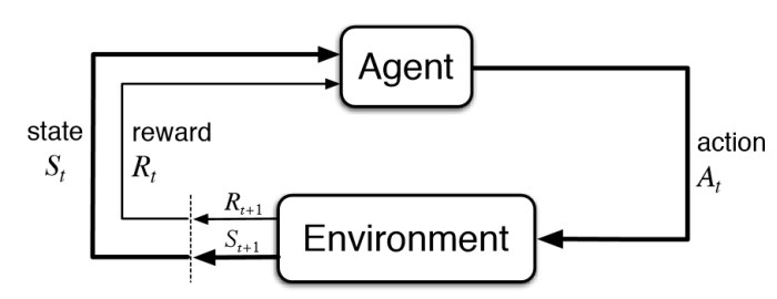
Figure 1: Basic reinforcement learning routine

The basic elements involved in reinforcement learning appears on Figure 1.

• An agent is something which interacts with the environment by executing certain actions, taking observations, and receiving eventual rewards for this. In most practical RL scenarios, it’s our piece of software that is supposed to solve some problem in an efficient way.

• The environment is external to an agent, and its communication with the environment is limited by rewards (obtained from the environment), actions (executed by the agent and given to the environment), and observations (some information besides the rewards that the agent receives from the environment and that defines a state).

  • An environment is said deterministic when any action has a single guaranteed effect, and no failure or uncertainty. On the contrary it is said non-deterministic. In this environment, the same task performed twice may produce different results or may even fail completely.

  • An environment is said episodic when each agent’s performance is the result of a series of independent tasks performed (episodes). There is no link between the agent’s performance and other different episodes.

  • A discrete environment has fixed locations or time intervals, while a continuous environment could be measured quantitatively to any level of precision.

• Actions are things that an agent can do in the environment. In RL, there are two types of actions: discrete or continuous. Discrete actions form a discrete set of mutually exclusive things an agent could do at one step, such as move left or right. But many real-world problems require the agent to take actions belonging to a continuous set, for instance choosing an angle or an acceleration when controlling a car.

• A reward is a scalar value agent obtains periodically from the environment. It can be positive or negative, large or small. The purpose of reward is to tell our agent how well it has behaved.

• Observations of the environment is the second information channel for an agent, with the first being the reward. As shown by $\textnormal{Figure }2$ & $3$ below, states and observations may not be the same. The environment state $S_{t}^{e}$ is the environment’s private representation, i.e. whatever data the environment uses to pick the next observation/reward. The environment state is not usually visible to the agent and may contain irrelevant information. The agent state $S^{a}_{t}$ is the agent’s internal representation, i.e. it is the information used by reinforcement learning algorithms. It can be any function of history $H_{t}=O_{1},R_{1},A_{1},...O_{t},R_{t}$: $S^{a}_{t}=f(H_{t})$

  

  Figure 2: Environment state

  

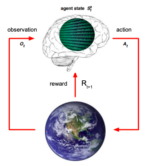
  Figure 3: Agent state

  We can then talk of Fully Observable Environments when the agent directly observes environment state: $O_{t}=S^{a}_{t}=S^{e}_{t}$. In this case we can use Markov decision process (MDP) model.

  When the environment is only partially observable by the agent (e.g. poker playing agent only observes public cards) we talk of Partially Observable Environments and use Partially observable Markov decision process (POMDP) model.

Figure 1 shows that in Fully Observable Environments, at each time step, the agent, knowing the current state, picks an action that modifies its environment. The agent receives an instantaneous reward depending on the action it chose, and receives information from the environment about the new state. Problems with these characteristics are best described in the framework of Markovian Decision Processes (MDPs).

2.1.2 Markov decision processes

Markov decision processes (MDP) formally describes an environment for reinforcement learning when the environment is fully observable. A MDP is a tuple $\left\langle\mathcal{S},\mathcal{A},P,R,\gamma\right\rangle$, where :

• $\mathcal{S}$ is the state space.

• $\mathcal{A}$ is the action space.

• $P$ is the state transition probability kernel

• $R$ is the reward function, $R:\mathcal{S}\times\mathcal{A}\to\mathbb{R}$

• $\gamma\in(0,1)$ is an optional discount factor.

In this work, we assume that $\mathcal{S}$ is finite and $\mathcal{A}$ is continuous. The markovian dynamics of the system is captured by $P$, since $P(s_{t+1}|s_{t},a_{t})$ is a stationary transition dynamics distribution with conditional probability verifying the Markov property: $P(s_{t+1}|s_{0},a_{0},\dots,s_{t},a_{t})=P(s_{t+1}|s_{t},a_{t})$.

As the agent selects an action $a_{t}$ at each step $t$ based on the current state $s_{t}$ and receives a reward $r_{t+1}$ (whose expectency is given by $R(s_{t},a_{t})$), there is a random state-action-reward sequence $\left(s_{t},a_{t},r_{t+1}\right)_{t\geq 0}$ corresponding to the agent’s behavior. A rule describing the way the actions are selected is called a policy. In the general case, an agent’s policy is stochastic and associates to each state $\mathcal{S}$ a distribution over $\mathcal{A}$. A particular case that we will further explore is the use of a deterministic policy, i.e., policy matching an action to each state. Dealing with such policy can be useful when the action space is very large or continuous.

Reinforcement learning methods specify how the agent’s policy should change to maximize an objective function. Let $\pi$ be the agent’s policy, then there are two classical ways of formulating the agent’s objective. One is the long-run average reward formulation, in which policies are ranked according to their long-term expected reward per step, $J(\pi)$ as:

$$J(\pi)=\underset{T}{\textnormal{ lim }}\frac{1}{T}\mathbb{E}\left[\sum_{t=0}^{T-1}\bar{r}_{t+1}\right]=\mathbb{E}_{s\sim d^{\pi},a\sim\pi(\cdot|s)}\left[R(s,a)\right]$$ (1)

where $d^{\pi}$ is the stationary distribution over states induced by $P^{\pi}$ giving the probability of transitioning from state $s$ to state $s^{\prime}$ following $\pi$: $P^{\pi}_{s,s^{\prime}}=\int_{\mathcal{A}}\pi(a|s)P(s^{\prime}|s,a)\textnormal{d}a$ (where $\pi$ can be viewed as a Dirac distribution if it is deterministic). We will make assumptions to ensure that $d^{\pi}$ is properly defined and does not depend on the initial state.

The second formulation requires to set a start state $s_{0}$ (or an initial state distribution $d_{0}$), and to care only about the discounted long-term reward obtained from it:

$$J(\pi)=\mathbb{E}_{a_{t}\sim\pi(\cdot|s_{t})}\left[\sum_{t=1}^{+\infty}\gamma^{t-1}r_{t}|s_{0}\right]$$

where $\gamma$ is a discount rate ($\gamma=1$ is allowed only in episodic tasks) granting less importance to rewards far in the future. This can be interpreted as a depreciation due to uncertainty of future rewards.

It could be tempting to view the average reward problem as a discounted reward problem in which the discounting factor tends to $1$ (when renormalizing by $(1-\gamma))$. However, it has been shown in Puterman:1994:MDP p. $165$ that for some converging algorithms the convergence rates can become very small as the discounting factor approaches $1$, therefore it makes sense to develop the theory of average reward algorithms separately. Thus, following Bhatnagar:2009:NaturalActorCritic; Prabuchandran:2016:A-C_Online_Feature_Adapt; FDMARL; Zhang:2018:ContinuousFDMARL, we will only consider the average reward setting in our theoretical developments.

Adopting this setting, we can introduce the differential action-value function $Q_{\pi}:\mathcal{S}\times\mathcal{A}\to\mathbb{R}$ Puterman:1994:MDP that gives the relative advantage of being in a state $s$ and taking an action $a$ when following a policy $\pi$:

$$Q_{\pi}(s,a)=\sum_{t=0}^{\infty}\mathbb{E}_{a\sim\pi(\cdot|s)}\left(r(s_{t},a_{t})-J(\pi)|s_{0}=s,a_{0}=a\right)$$

Similarly, the differential value-function $V_{\pi}:\mathcal{S}\to\mathbb{R}$ giving the relative advantage of being in a state $s$ when following a policy $\pi$ is defined as:

$$V_{\pi}(s,a)=\sum_{t=0}^{\infty}\mathbb{E}_{a\sim\pi(\cdot|s)}\left(r(s_{t},a_{t})-J(\pi)|s_{0}=s\right)$$

For simplicity, we will hereafter refer to $Q_{\pi}$ and $V_{\pi}$ as respectively value function and state-value function.

Since in many problems of interest, the number of states is very large (for example, in games such as Backgammon, Chess, and $19\times 19$ computer Go, there are roughly 1028, 1047 and 10170 states, respectively) and since here the action space is continuous, we cannot hope to compute value functions exactly and instead use approximation techniques. We will approximate $Q_{\pi}$ by some parametrized functions $\hat{Q}^{\pi}_{\omega}$ with parameter $\omega$. For notational convenience we write $\hat{Q}_{\omega}$ when there is no ambiguity on the underlying policy. Similarly, a policy $\pi$ can also be parametrized as $\pi_{\theta}$ (one can think of a standard Gaussian policy with mean $\theta$), in which case the reinforcement learning algorithm’s goal is to find the best admissible $\theta$ maximizing $J(\pi_{\theta})$. This is a model free problem given that we don’t have a direct access to the environment’s dynamics characterized by $P$. One of the most important information on $Q_{\pi}$ is that it verifies the Bellman equation (also known as the Poisson equation) Puterman:1994:MDP:

$$Q_{\pi}(s,a)=R(s,a)+\sum_{s^{\prime}\in\mathcal{S}}P^{\pi_{\theta}}(s^{\prime}|s)V_{\pi}(s^{\prime})$$ (2)

Therefore a classical idea to find a good approximation of the value function is to choose $\omega$ by minimizing at each step $t$, the temporal-difference error

$$\delta_{t}=|(r_{t+1}-J(\pi_{\theta})+\hat{Q}_{\omega}(s_{t+1},a_{t+1}))-\hat{Q}_{\omega}(s_{t},a_{t})|$$ (3)

is small.

Now that the main elements of single-agent RL machinery are introduced, we can straightforwardly extend them to the decentralized multi-agent setting.

2.2 Decentralized Multi-Agent Reinforcement Learning

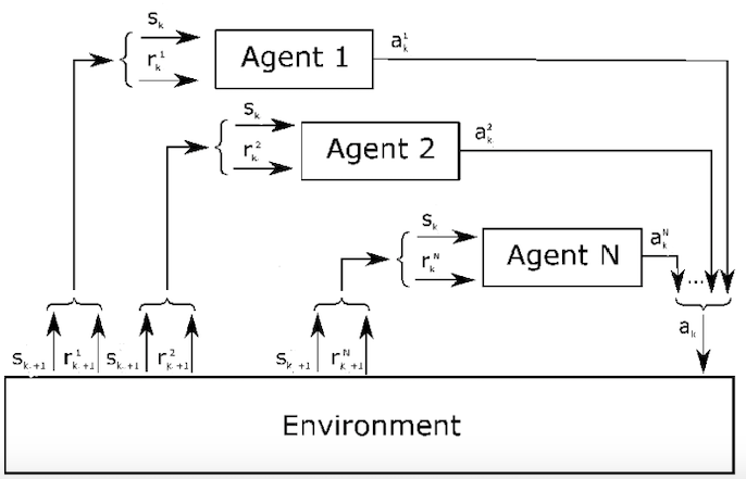
Figure 4: Decentralized MARL routine

We consider now a system of $N$ agents denoted by $\mathcal{N}=\left\llbracket 1,n\right\rrbracket$ operating in a common environment. As in FDMARL; Suttle:2019:MA-OFF-Policy-AC, we model multi-agent reinforcement learning problem as a networked multi-agent MDP described by a tuple $\left\langle\mathcal{S},\mathcal{A},P,\left\{R^{i}\right\}_{i\in\mathcal{N}},\left\{\mathcal{G}_{t}\right\}_{t\geq 0}\right\rangle$ where

• $\mathcal{S}$ is a finite state space.

• $\mathcal{A}=\prod_{i\in\mathcal{N}}\mathcal{A}^{i}$ is a joint action space (where $\mathcal{A}^{i}$ is the continuous action space associated to agent $i$).

• $P$ is the same as in the single agent setting.

• $\left\{R^{i}\right\}_{i\in\mathcal{N}}$ is the set of local reward functions $R^{i}:\mathcal{S}\times\mathcal{A}\to\mathbb{R}$

• $\left\{\mathcal{G}_{t}\right\}_{t}=\left\{\left(\mathcal{N},\mathcal{E}_{t}\right)\right\}_{t}$ is a sequence of time-varying communication networks

Throughout this report, it is assumed that states and actions are globally observed but that rewards are only locally observed, i.e., $r^{i}_{t}$ is only known by agent $i$. The process is thus decentralized in the sense that no central controller either collects local rewards or takes actions on behalf of the agents. The communication network is modelled as a time-varying graph $\mathcal{G}_{t}=\left(\mathcal{N},\mathcal{E}_{t}\right)$ where $\mathcal{E}_{t}$ denotes the edge set of $\mathcal{G}_{t}$. Agents $i$ and $j$ can share some information at time $t$ if and only if $(i,j)$ is in $\mathcal{E}_{t}$.

As action selection is performed locally by each agent, we can assume that this selection is conditionally independent given the current state. So with this decentralized setting, we can express a joint policy $\pi$ as a product of the local policies $\pi^{i}$: $\pi(a|s)=\prod_{i\in\mathcal{N}}\pi^{i}(a^{i}|s)$ where $a=(a_{1},\dots,a_{N})\in\mathcal{A}$ and $\pi^{i}(a^{i}|s)$ is the conditional probability density of $a^{i}$ associated with the policy $\pi^{i}$ of agent $i$. At step $t$, given the global state $s_{t}$, agents select $a_{t}=(a^{1}_{t},\dots,a^{N}_{t})$ according to their own policy, and as a result, each agent receives a specific reward $r^{i}_{t+1}$ whose expected value is given by $R^{i}(s_{t},a_{t})$ (the local reward depends on the state and the global action). Thus decentralized setting allows to handle the case of multi-tasks RL Macua:2017:Dec_multi-task_deep-RL as local rewards can be totally unrelated to one another.

We now assume that each agent follows a deterministic policy $\mu^{i}_{\theta^{i}}:\mathcal{S}\to\mathcal{A}$ parametrized by $\theta^{i}\in\Theta^{i}$, with $\Theta^{i}$ a compact subset of $\mathbb{R}^{m_{i}}$. Then $\mu_{\theta}:\mathcal{S}\to\mathcal{A}$ defined as $\mu_{\theta}(s)=\left(\mu_{\theta}^{1}(s),\dots,\mu_{\theta}^{N}(s)\right)=\left(\mu_{\theta^{1}}^{1}(s),\dots,\mu_{\theta^{N}}^{N}(s)\right)$, with $\theta=\big{[}\left(\theta^{1}\right)^{\top},\dots,\left(\theta^{N}\right)^{\top}]^{\top}\in\mathbb{R}^{m}$ is the joint policy of all agents and we have $a_{t}=\mu_{\theta}(s_{t})$. We note $\bar{r}_{t}$ the reward averaged over all agents, i.e., $\bar{r}_{t}=\frac{1}{N}\sum_{i\in\mathcal{N}}r^{i}_{t}$, and similarly, we note $\bar{R}(s,a)=\frac{1}{N}\sum_{i\in\mathcal{N}}R^{i}(s,a)$.

The following is a regularity assumption on the networked MDP and policy function that is standard in existing work on actor-critic algorithms using function approximation Konda:Tsitsiklis:actor-criticalgorithms; Bhatnagar:2009:NaturalActorCritic.

Assumption 2.1.

For any $i\in\mathcal{N},s\in\mathcal{S},\mu^{i}_{\theta^{i}}(s)$ is twice continuously differentiable with respect to the parameter $\theta^{i}$ over $\Theta^{i}$. Moreover, for any $\theta\in\Theta$, let $P^{\theta}$ be the transition matrix of the Markov chain $\{s_{t}\}_{t\geq 0}$ induced by policy $\mu_{\theta}$, that is

$$P^{\mu_{\theta}}(s^{\prime}|s)=P(s^{\prime}|s,\mu_{\theta}(s)),\quad\forall s,s^{\prime}\in\mathcal{S}$$

We assume that the Markov chain $\{s_{t}\}_{t\geq 0}$ is irreducible and aperiodic under any $\mu_{\theta}$, $\theta\in\Theta$ and denote by $d^{\mu}_{\theta}$ its stationary distribution. Furthermore, we assume that $r^{i}(s,a)$ is uniformly bounded for all $i\in\mathcal{N},s\in\mathcal{S},a\in\mathcal{A}$.

In addition we make another standard assumption regarding the regularity of the expected reward $R^{i}$ and the state transition probability kernel $P$.

Assumption 2.2.

For any $s,s^{\prime}\in\mathcal{S},i\in\mathcal{N}$, $P(s^{\prime}|s,a)$ and $R^{i}(s,a)$ are bounded, twice differentiable, and have bounded first and second derivatives.

This assumption will allows to justify the existence and differentiability of the cooperative objective function that the agents aim at maximizing. In the multi-agent setting, this objective function is the long-run average reward given by $J(\mu_{\theta})$:

$$J(\mu_{\theta}) =\underset{T}{\textnormal{ lim }}\frac{1}{T}\mathbb{E}\left[\sum_{t=0}^{T-1}\bar{r}_{t+1}\right]=\mathbb{E}_{s\sim d^{\theta}}\left[\bar{R}(s,\mu_{\theta}(s))\right]$$ (4)

Similar to the single-agent case, we define the action-value function $Q_{\mu_{\theta}}:\mathcal{S}\times\mathcal{A}\to\mathbb{R}$ and value function $V_{\mu_{\theta}}:\mathcal{S}\to\mathbb{R}$ as follow:

$$Q_{\mu_{\theta}}(s,a)=\sum_{t=0}^{\infty}\mathbb{E}\left(\bar{r}(s_{t},a_{t})-J(\mu_{\theta})|s_{0}=s,a_{0}=a,\mu_{\theta}\right)$$ (5)

$$V_{\mu_{\theta}}(s)=\sum_{t=0}^{\infty}\mathbb{E}\left(\bar{r}(s_{t},a_{t})-J(\mu_{\theta})|s_{0}=s,\mu_{\theta}\right)$$ (6)

Note that, for deterministic policy $\mu_{\theta}$, there is a simple relation between $V_{\mu_{\theta}}$ and $Q_{\mu_{\theta}}$:

$$V_{\theta}(s)=Q_{\theta}(s,\mu_{\theta}(s))$$ (7)

and the Poisson equation (2) becomes:

$$Q_{\mu_{\theta}}(s,a)=\bar{R}(s,a)-J(\mu_{\theta})+\sum_{s^{\prime}\in\mathcal{S}}P(s^{\prime}|s,\mu_{\theta}(s))Q(s^{\prime},\mu_{\theta}(s^{\prime}))$$ (8)

Now that the RL formalism has been introduced, we can try to solve our RL problem by adapting a popular algorithm called Actor-Critic (AC) to our deterministic multi-agent setting.

3 Actor-Critic algorithm

We first present Actor-Critic principle for the single-agent case before naturally extending it to the multi-agent setting.

3.1 Principle

Given a parametrized policy $\mu_{\theta}$, Actor-only methods Marbach:2001 consist in estimating the gradient of the objective function $J(\mu_{\theta})$ with respect to the actor parameter $\theta$, and to update this parameter following a gradient-ascent direction. As this estimation is done after each iteration of $\theta$, theoretical and empirical studies emphasized an important drawback of these methods, which is the high variance of their gradient estimators, which can lead to slower convergence and sample inefficiency. On the other hand, a Critic-only method aims at learning an approximate solution to the Bellman equation associated to $Q_{\mu_{\theta}}$ or $V_{\mu_{\theta}}$. There is no update of $\theta$, so the goal of these methods is not to improve the policy but to have a good estimation of its performance.

Combining the strengths of both methods, Actor-Critic algorithm has been proposed in Konda:Tsitsiklis:actor-criticalgorithms to find the optimal policy following a gradient ascent strategy based on a better estimation of the value functions.

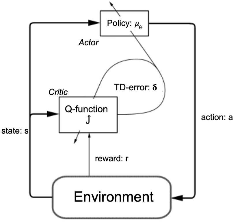
Figure 5: Actor-Critic routine

Figure 5 shows the algorithm routine with a single agent:

• In the critic step, based on the observation of $s_{t},a_{t},r_{t+1}$ and $s_{t+1}$ the $Q$-function parameter $\omega$ is updated based on a Temporal-Difference scheme (3) requiring the estimation of the long-run average reward $\hat{J}$, which is updated as well.

• In the actor step, the policy parameter $\theta$ is updated following the estimation of the gradient of $J$.

Updating $\theta$, $\hat{J}$, $\omega$ by directly interacting with the environment following the current policy (i.e. in an on-line fashion), we can hope to get eventually a good estimate parameter for $Q_{\mu_{\theta}}$ where $\theta$ is close to to a local optimizer of the true objective function $J(\mu_{\theta})$.

3.2 Critic step: Temporal Difference learning (TD)

Part of the RL literature has focused on the estimation of the objective function, state value function or action value function associated to a stationary policy. This problem arises as a subroutine of generalized policy iteration and is generally thought to be an important step in developing algorithms that can learn good control policies in reinforcement learning. Considering a stationary policy $\mu_{\theta}$, estimate the objective function $J(\mu_{\theta})=\mathbb{E}_{s\sim d^{\mu_{\theta}}}\left[R(s,\mu_{\theta}(s))\right]$ by some $\hat{J}_{t}$ relies on a classical stochastic approximation approach Robbins&Monro:1951:

$$\hat{J}_{t+1}=\hat{J}_{t}+\beta_{J,t}(r_{t+1}-\hat{J}_{t})$$ (9)

where $\beta_{J,t}$ belongs to a family of vanishing step-sizes characterized in Assumption 4.8. Note that, with $\beta_{J,t}=\frac{1}{t+1}$ we have

$$\hat{J}_{t}=\frac{1}{t}\hat{J}_{0}+\frac{1}{t}\sum_{k=0}^{t-1}r_{k+1}\to J(\mu_{\theta})\quad\textnormal{a.s.}$$

For the action value function estimation, we consider the simpler TD learning version, called TD($0$) (generalized as TD($\lambda$) with $\lambda\in\left[0,1\right]$ Sutton:1988:RL_TD), which is based on the one-step error signal (3). This method somehow has the flavor of supervised learning, as the goal is to minimize an error measure with respect to some set of values that parameterizes the function making the prediction. Here, the predicting function is the parametrized value-function $\hat{Q}_{\omega_{t}}$, and, given the sequence $s_{t},a_{t},r_{t+1},s_{t+1}anda_{t+1}$, the predicted value $\hat{Q}_{\omega}(s_{t},a_{t})$ is compared to the target value $r_{t+1}-\hat{J}_{t}+\hat{Q}_{\omega_{t}}(s_{t+1},a_{t+1})$ (Owing to the Poisson equation (2)). As the predicting function is also used to define the target value, TD($0$) is called a bootstrapping method. Nonetheless, as in supervised learning, the one-step gradient descent is performed considering the target value fixed, which gives $\omega_{t}$ update:

$$\omega_{t+1}=\omega_{t}+\beta_{\omega,t}\cdot\left(r_{t+1}-\hat{J}_{t}+\hat{Q}_{\omega_{t}}(s_{t+1},a_{t+1})-\hat{Q}_{\omega_{t}}(s_{t},a_{t})\right)\cdot\left.\nabla_{\omega}\hat{Q}_{\omega}(s_{t},a_{t})\right|_{\omega=\omega_{t}}$$ (10)

It is classical to set $\beta_{J,t}=\beta_{\omega,t}$, so finally we have the following critic recursion

$$\hat{J}_{t+1}=\hat{J}_{t}+\beta_{\omega,t}(r_{t+1}-\hat{J}_{t})$$ (11)

$$\omega_{t+1}=\omega_{t}+\beta_{\omega,t}\cdot\delta_{t}\cdot\left.\nabla_{\omega}\hat{Q}_{\omega}(s_{t},a_{t})\right|_{\omega=\omega_{t}}$$ (12)

with $\delta_{t}=r_{t+1}-\hat{J}_{t}+\hat{Q}_{\omega_{t}}(s_{t+1},a_{t+1})-\hat{Q}_{\omega_{t}}(s_{t},a_{t})$.

We now need to focus on the actor step, which is a gradient ascent method, requiring an estimation of the gradient of $J(\mu_{\theta})$. In RL literature, this is referred to as a policy gradient problem.

3.3 Actor step: Policy Gradient (PG)

The fundamental result underlying the actor step of an AC algorithm is the policy gradient theorem Sutton:2000:Policy_grad_meth_RL_fct_appr giving a simple expression of the gradient of the objective function $J(\pi_{\theta})$ for a parametrized stochastic policy $\pi_{\theta}$ in the case of both discounted and undiscounted MDP (specific assumptions will be made when giving our policy gradient result in theorem 3.1):

$$\nabla_{\theta}J(\pi_{\theta})=\sum_{s\in\mathcal{S}}\int_{\mathcal{A}}\nabla_{\theta}\pi_{\theta}(a|s)Q_{\pi}(s,a)\textnormal{d}a=\mathbb{E}_{s\sim d^{\pi_{\theta}},a\sim\pi_{\theta}}\left[\nabla_{\theta}\log\pi_{\theta}(a|s)Q_{\pi}(s,a)\right]$$ (13)

An interesting aspect of this formula comes from the fact that even though $J(\pi_{\theta})$ depends on the stationary distribution $d^{\pi_{\theta}}$, its gradient with respect to $\theta$ does not involve the gradient of this distribution, which is a good thing since it might be hard to approximate. In the discounted setting, there is a useful extension of this PG result to the case of a deterministic policy $\mu_{\theta}$ Silver:2014:DeterministicPolicyGradient:

$$\nabla_{\theta}J(\mu_{\theta})=\sum_{s\in\mathcal{S}}\nabla_{\theta}\mu_{\theta}(s)\left.\nabla_{a}Q_{\mu_{\theta}}(s,a)\right|_{a=\mu_{\theta}(s)}=\mathbb{E}_{s\sim d^{\mu_{\theta}}}\left[\nabla_{\theta}\mu_{\theta}(s)\left.\nabla_{a}Q_{\mu_{\theta}}(s,a)\right|_{a=\mu_{\theta}(s)}\right]$$ (14)

Similar to (13), gradient of $J$ with respect to $\theta$ is again independent of $\nabla_{\theta}d^{\pi_{\theta}}$.

To the best of our knowledge, no such expression for deterministic policy gradient has been provided in the undiscounted setting. As it is the case we want to handle, we show that (14) is still true in the long-run average reward setting (1):

Theorem 3.1 (Deterministic Policy Gradient Theorem).

For any $\theta\in\Theta$, under Assumptions 2.1 and 2.2 (here for $N=1$), $\nabla_{\theta}J(\mu_{\theta})$ exists and is given by

$$\nabla_{\theta}J(\mu_{\theta})=\mathbb{E}_{s\sim d^{\mu_{\theta}}}\left[\nabla_{\theta}\mu_{\theta}(s)\left.\nabla_{a}Q_{\mu_{\theta}}(s,a)\right|_{a=\mu_{\theta}(s)}\right]$$

Proof.

The proof follows the same scheme as Sutton:2000:Policy_grad_meth_RL_fct_appr, naturally extending their results for a deterministic policy $\mu_{\theta}$ and a continuous action space $\mathcal{A}$. Within this proof $J(\theta)$ (resp. $d^{\theta},Q_{\theta},V_{\theta}$) stands for $J_{\mu_{\theta}}$ (resp. $d^{\mu_{\theta}},Q_{\mu_{\theta}},V_{\mu_{\theta}}$).

Note that assumptions 2.1 and 2.2 ensures that, for any $s\in\mathcal{S}$, $V_{\theta}(s)$, $\nabla_{\theta}V_{\theta}(s)$, $J(\theta)$, $\nabla_{\theta}J(\theta)$, $d^{\theta}$(s) are Lipschitz-continuous functions of $\theta$, and that $Q_{\theta}(s,a)$ and $\nabla_{a}Q_{\theta}(s,a)$ are Lipschitz-continuous functions of $a$ (Marbach:2001). Taking the gradient on both sides of (7),

$$\nabla_{\theta}V_{\theta}(s) =\nabla_{\theta}Q_{\theta}(s,\mu_{\theta}(s))$$

$$=\nabla_{\theta}\big{[}\bar{R}(s,\mu_{\theta}(s))-J(\theta)+\sum_{s^{\prime}\in\mathcal{S}}P(s^{\prime}|s,\mu_{\theta}(s))V_{\theta}(s^{\prime})\big{]}$$

$$=\nabla_{\theta}\mu_{\theta}(s)\left.\nabla_{a}\bar{R}(s,a)\right|_{a=\mu_{\theta}(s)}-\nabla_{\theta}J(\theta)+\nabla_{\theta}\sum_{s^{\prime}\in\mathcal{S}}P(s^{\prime}|s,\mu_{\theta}(s))V_{\theta}(s^{\prime})$$

$$\begin{split}&=\nabla_{\theta}\mu_{\theta}(s)\left.\nabla_{a}\bar{R}(s,a)\right|_{a=\mu_{\theta}(s)}-\nabla_{\theta}J(\theta)\\ &\qquad+\sum_{s^{\prime}\in\mathcal{S}}\nabla_{\theta}\mu_{\theta}(s)\left.\nabla_{a}P(s^{\prime}|s,a)\right|_{a=\mu_{\theta}(s)}V_{\theta}(s^{\prime})+\sum_{s^{\prime}\in\mathcal{S}}P(s^{\prime}|s,\mu_{\theta}(s))\nabla_{\theta}V_{\theta}(s^{\prime})\end{split}$$

$$\begin{split}&=\nabla_{\theta}\mu_{\theta}(s)\nabla_{a}\left.\Big{[}\bar{R}(s,a)+\sum_{s^{\prime}\in\mathcal{S}}P(s|s^{\prime},a)V_{\theta}(s^{\prime})\Big{]}\right|_{a=\mu_{\theta}(s)}\\ &\qquad-\nabla_{\theta}J(\theta)+\sum_{s^{\prime}\in\mathcal{S}}P(s^{\prime}|s,a)\nabla_{\theta}V_{\theta}(s^{\prime})\end{split}$$

$$=\nabla_{\theta}\mu_{\theta}(s)\nabla_{a}\left.Q_{\theta}(s,a)\right|_{a=\mu_{\theta}(s)}+\sum_{s^{\prime}\in\mathcal{S}}P(s^{\prime}|s,\mu_{\theta}(s))\nabla_{\theta}V_{\theta}(s^{\prime})-\nabla_{\theta}J(\theta)$$

Hence,

$$\nabla_{\theta}J(\theta) =\nabla_{\theta}\mu_{\theta}(s)\nabla_{a}\left.Q_{\theta}(s,a)\right|_{a=\mu_{\theta}(s)}+\sum_{s^{\prime}\in\mathcal{S}}P(s^{\prime}|s,\mu_{\theta}(s))\nabla_{\theta}V_{\theta}(s^{\prime})-\nabla_{\theta}V_{\theta}(s)$$

$$\begin{split}\sum_{s\in\mathcal{S}}d^{\theta}(s)\nabla_{\theta}J(\theta)&=\sum_{s\in\mathcal{S}}d^{\theta}(s)\nabla_{\theta}\mu_{\theta}(s)\nabla_{a}\left.Q_{\theta}(s,a)\right|_{a=\mu_{\theta}(s)}\\ &\qquad+\sum_{s\in\mathcal{S}}d^{\theta}(s)\sum_{s^{\prime}\in\mathcal{S}}P(s^{\prime}|s,\mu_{\theta}(s))\nabla_{\theta}V_{\theta}(s^{\prime})-\sum_{s\in\mathcal{S}}d^{\theta}(s)\nabla_{\theta}V_{\theta}(s)\end{split}$$

Using stationarity property of $d^{\theta}$, we get

$$\sum_{s\in\mathcal{S}}\sum_{s^{\prime}\in\mathcal{S}}d^{\theta}(s)P(s^{\prime}|s,\mu_{\theta}(s))\nabla_{\theta}V_{\theta}(s^{\prime})=\sum_{s^{\prime}\in\mathcal{S}}d^{\theta}(s^{\prime})\nabla_{\theta}V_{\theta}(s^{\prime})$$

Thus

$$\nabla_{\theta}J(\theta)=\sum_{s\in\mathcal{S}}d^{\theta}(s)\nabla_{\theta}\mu_{\theta}(s)\left.\nabla_{a}Q_{\theta}(s,a)\right|_{a=\mu_{\theta}(s)}=\mathbb{E}_{s\sim d^{\theta}}\big{[}\nabla_{\theta}\mu_{\theta}(s)\left.\nabla_{a}Q_{\theta}(s,a)\right|_{a=\mu_{\theta}(s)}]$$

∎

Even though stochastic (13) and deterministic (14) policy gradients may not look alike at first glance, it has been established in Silver:2014:DeterministicPolicyGradient, that for a wide class of stochastic policies, the deterministic policy gradient is a limiting case of the stochastic policy gradient. The claim is that, in a discounted setting, if we consider parametrized stochastic policies $\pi_{\mu,\sigma}$ associated to deterministic policies $\mu_{\theta}$ where $\sigma$ is a variance parameter and such that, when $\sigma\to 0$, we have $\pi_{\theta,\sigma\downarrow 0}\equiv\mu_{\theta}$ then the stochastic policy gradient converges to the deterministic gradient. We prove that this limit still holds under the long-run average setting:

Theorem 3.2.

Let $\pi_{\theta,\sigma}$ stochastic policy such that $\pi_{\theta,\sigma}(a|s)=\nu_{\sigma}(\mu_{\theta}(s),a)$, where $\sigma$ is a parameter controlling the variance, and $\nu_{\sigma}$ satisfy conditions A.1. Suppose further that the Assumptions 2.1 and 2.2 on the MDP hold. Then,

$$\underset{\sigma\downarrow 0}{\textnormal{lim }}\nabla_{\theta}J_{\pi_{\theta,\sigma}}(\pi_{\theta,\sigma})=\nabla_{\theta}J_{\mu_{\theta}}(\mu_{\theta})$$ (15)

where on the l.h.s the gradient is the standard stochastic policy gradient (13) and on the r.h.s. the gradient is the deterministic policy gradient given in Theorem 3.1.

The proof does not rely on the expressions of the policy gradient given by (13) and (15), but by directly applying gradient operator to the definition of $J$ (which, for the deterministic case (1), gives:

$$\nabla_{\theta}J(\mu_{\theta})=\sum_{s\in\mathcal{S}}\nabla_{\theta}d^{\mu_{\theta}}(s)\bar{R}(s,\mu_{\theta}(s))+\sum_{s\in\mathcal{S}}d^{\mu_{\theta}}(s)\nabla_{\theta}\mu_{\theta}(s)\left.\nabla_{a}\bar{R}(s,a)\right|_{a=\mu_{\theta}(s)}$$

by simple differentiation of a product). We then use that the gradient of $d^{\pi_{\theta,\sigma}}$ converges towards the gradient of $d^{\mu_{\theta}}$ as $\sigma\downarrow 0$ under some technical conditions and exploit properties of $\nu_{\sigma}$. A rigorous statement of this theorem and details of the proof are provided in Appendix A.1.

It has been emphasized in Silver:2014:DeterministicPolicyGradient that the fact that deterministic gradient is a limit case of the stochastic gradient makes it likely that standard machinery of policy gradient, such as compatible-function approximation Sutton:2000:Policy_grad_meth_RL_fct_appr, natural gradients Kakade:2001:NPG, on-line feature adaptation Prabuchandran:2016:A-C_Online_Feature_Adapt, and also actor-critic Konda:2002:Actor-Critic could be still applicable when having deterministic policy. That is why it was important to show that this convergence held in the long-run average setting.

Having an expression for the deterministic policy gradient (15), we can use it to design the actor step of our actor-critic algorithm as follows:

$$\theta_{t+1}=\theta_{t}+\beta_{\theta,t}\cdot\nabla_{\theta}\mu_{\theta_{t}}(s_{t})\cdot\left.\nabla_{a}Q_{\omega_{t}}(s_{t},a_{t})\right|_{a=\mu_{\theta_{t}(s_{t})}}$$ (16)

We get an actor-critic algorithm by iterating $(\ref{algo:critic-step-single-agent})$ and (16) on a sequence of states $s_{t}$, actions $\mu_{\theta_{t}}(s_{t})$ and rewards $r_{t+1}$ generated by interacting with the environment.

3.4 Actor-Critic algorithm for Decentralized-MARL

In this section, we adapt the actor-critic algorithm presented above for the multi-agent MDP with networked agents. Each agent follows a parametrized deterministic policy $\mu^{i}_{\theta^{i}}$.

3.4.1 Critic step

As in FDMARL, we assume that each agent $i$ maintains its own parameter $\omega^{i}$ and uses $Q_{\omega^{i}}$ as a local estimate of the global value function $Q_{\mu_{\theta}}$ defined as (5). Parameters $\omega^{i}$ is a column vector of $\mathbb{R}^{K}$ that will be updated at each time-step during the critic step. Since in the multi-agent setting the Bellman equation involves the globally averaged reward $\bar{r}_{t+1}$, estimation of $Q_{\mu_{\theta}}$ requires aggregation of local information, as if agents share no information then they won’t be able to learn anything apart from maximizing their own rewards which may lead to a bad averaged reward. Thus, the communication network is used by each agent $i$ to share its local parameter $\omega^{i}$ with its neighbors, so that a consensus can be reached upon the parameter $\omega$ that provides the best approximation of $Q_{\mu_{\theta}}$. Note that this communication does not compromise agent’s confidentiality, as it is not possible to infer either $r^{i}$ or $\theta^{i}$ from the sharing of $\omega^{i}$.

The critic update is comprised of two steps: an update similar to the single-agent critic step based on TD($0$) for the action value function and classical stochastic approximation for the local long-run expected reward, and a consensus step during which each agent updates its local parameter $\omega$ by taking a linear combination of its neighbors parameter estimates. Weights associated to this combination is governed by $C_{t}=(c_{t}^{ij})_{ij}\in\mathbb{R}_{+}^{N\times N}$ where $c_{t}^{ij}$ denotes the weight on the message transmitted from $i$ to $j$ at time $t$. This weight matrix depends on $\mathcal{G}_{t}$ in a way that is described in assumption 4.7. Thus, the critic step is as follows,

$$\hat{J}_{t+1}^{i}=(1-\beta_{\omega,t})\cdot\hat{J}_{t}^{i}+\beta_{\omega,t}\cdot r_{t+1}^{i}\hskip 20.00003pt \widetilde{\omega}^{i}_{t}=\omega_{t}^{i}+\beta_{\omega,t}\cdot\delta_{t}^{i}\cdot\left.\nabla_{\omega}\hat{Q}_{\omega^{i}}(s_{t},a_{t})\right|_{\omega=\omega^{i}_{t}}\hskip 10.00002pt \omega_{t+1}^{i}=\sum_{j\in\mathcal{N}}c_{t}^{ij}\cdot\widetilde{\omega}^{j}_{t}$$ (17)

with

$$\delta_{t}^{i}=r_{t+1}^{i}-\hat{J}_{t}^{i}+\hat{Q}_{\omega_{t}^{i}}(s_{t+1},a_{t+1})-\hat{Q}_{\omega_{t}^{i}}(s_{t},a_{t})$$

where $\hat{J}^{i}$ is updated with the same learning rate as $\omega^{i}$ Konda:2002:Actor-Critic. $\tilde{\omega}$ is an auxiliary parameter updated according to TD($0$), and then $\omega^{i}$ is updated through consensus step.

3.4.2 Actor step

As done in FDMARL, we derive a multi-agent policy gradient directly from the single agent expression (15).

Theorem 3.3 (Local Deterministic Policy Gradient Theorem - On Policy).

For any $\theta\in\Theta$, $i\in\mathcal{N}$, under Assumptions 2.1 and 2.2, $\nabla_{\theta^{i}}J(\theta)$ exists and is given by

$$\nabla_{\theta^{i}}J(\theta)=\mathbb{E}_{s\sim d^{\theta}}\left[\nabla_{\theta^{i}}\mu^{i}_{\theta^{i}}(s)\nabla_{a^{i}}\left.Q_{\theta}(s,\mu^{-i}_{\theta^{-i}}(s),a^{i})\right|_{a^{i}=\mu^{i}_{\theta^{i}}(s)}\right]$$ (18)

Proof.

Having $\mu_{\theta}(s)=\left(\mu_{\theta}^{1}(s),\dots,\mu_{\theta}^{N}(s)\right)=\left(\mu_{\theta^{1}}^{1}(s),\dots,\mu_{\theta^{N}}^{N}(s)\right)$, with $\theta=\big{[}\left(\theta^{1}\right)^{\top},\dots,\left(\theta^{N}\right)^{\top}]^{\top}$, we have from the single-agent policy gradient (15):

$$\nabla_{\theta}J(\mu_{\theta})=.\mathbb{E}_{s\sim d^{\mu_{\theta}}}\left[\nabla_{\theta}\mu_{\theta}(s)\cdot\left.\nabla_{a}Q(s,a)\right|_{a=\mu_{\theta}(s)}\right]$$

Given that $\nabla_{\theta^{i}}\mu_{\theta}^{j}(s)=0$ if $i\neq j$, we have $\nabla_{\theta}\mu_{\theta}(s)=\textnormal{Diag}(\nabla_{\theta^{1}}\mu_{\theta_{1}}^{1}(s),\dots,\nabla_{\theta^{N}}\mu_{\theta_{N}}^{N}(s))$, and (18) directly follows. ∎

This shows, that the gradient of the objective function with respect to the local parameter $\theta^{i}$ can be obtained locally as it depends on the local gradient $\nabla_{\theta^{i}}\mu^{\theta^{i}}_{\theta^{i}}$ and on the global action-value function that can be approximated locally by $\hat{Q}_{\omega^{i}}$. This property is one of the key aspects of decentralized actor critic algorithm FDMARL; Zhang:2018:ContinuousFDMARL; Suttle:2019:MA-OFF-Policy-AC. Thus, we have the following actor step motivated by (18):

$$\theta^{i}_{t+1}=\theta_{t}^{i}+\beta_{\theta,t}\cdot\nabla_{\theta^{i}}\mu_{\theta^{i}_{t}}^{i}(s_{t})\cdot\left.\nabla_{a^{i}}\hat{Q}_{\omega^{i}_{t}}(s_{t},a^{-i}_{t},a^{i})\right|_{a^{i}=a^{i}_{t}}$$ (19)

Each agent $i$ updates its policy in direction of the estimated ascending gradient $\nabla_{\theta^{i}}J$ with learning rate $\beta_{\theta,t}$ smaller than $\beta_{\omega,t}$, as discussed below.

3.4.3 Pseudocode of Decentralized Actor-Critic

Having a critic and an actor step, we give in Algorithm 1 the pseudocode of the Decentralized Deterministic Multi-Agent Actor Critic we designed . Parts in red refer to the use of compatible function, as discussed in section 5.1.

Algorithm 1 Networked deterministic on-policy actor-critic algorithm based on action-value function

  Input: Initial values $\hat{J}_{0}^{i},\omega^{i}_{0},\widetilde{\omega}^{i}_{0},\theta_{0}^{i},\forall i\in\mathcal{N}$; $s_{0}$ initial state of the MDP, stepsizes $\{\beta_{\omega,t}\}_{t\geq 0},\{\beta_{\theta,t}\}_{t\geq 0}$

  Draw $a^{i}_{0}=\mu^{i}_{\theta^{i}_{0}}(s_{0})$ and compute $\widetilde{a}_{0}^{i}=\nabla_{\theta^{i}}\mu^{i}_{\theta^{i}_{0}}(s_{0})$

  Observe joint action $a_{0}=(a^{1}_{0},\dots,a^{N}_{0})$ and $\widetilde{a}_{0}=\left(\widetilde{a}^{1}_{0},\dots,\widetilde{a}^{N}_{0}\right)$

  repeat

     for $i\in\mathcal{N}$ do

        Observe $s_{t+1}$ and reward $r_{t+1}^{i}=r^{i}(s_{t},a_{t})$

        Update $\hat{J}^{i}_{t+1}\leftarrow(1-\beta_{\omega,t})\cdot\hat{J}_{t}^{i}+\beta_{\omega,t}\cdot r_{t+1}^{i}$

        Draw action $a_{t+1}=\mu^{i}_{\theta^{i}_{t}}(s_{t+1})$ and compute $\widetilde{a}_{t+1}^{i}=\nabla_{\theta^{i}}\mu^{i}_{\theta^{i}_{t}}(s_{t+1})$

     end for

     Observe joint action $a_{t+1}=(a^{1}_{t+1},\dots,a^{N}_{t+1})$ and $\widetilde{a}_{t+1}=\left(\widetilde{a}^{1}_{t+1},\dots,\widetilde{a}^{N}_{t+1}\right)$

     for $i\in\mathcal{N}$ do

        Update: $\delta_{t}^{i}\leftarrow r_{t+1}^{i}-\hat{J}_{t}^{i}+\hat{Q}_{\omega_{t}^{i}}(s_{t+1},a_{t+1})-\hat{Q}_{\omega_{t}^{i}}(s_{t},a_{t})$

        Critic step: $\widetilde{\omega}^{i}_{t}\leftarrow\omega_{t}^{i}+\beta_{\omega,t}\cdot\delta_{t}^{i}\cdot\left.\nabla_{\omega}\hat{Q}_{\omega^{i}}(s_{t},a_{t})\right|_{\omega=\omega^{i}_{t}}$

        Actor step: $\theta^{i}_{t+1}=\theta_{t}^{i}+\beta_{\theta,t}\cdot\nabla_{\theta^{i}}\mu_{\theta^{i}_{t}}^{i}(s_{t})\left.\nabla_{a^{i}}\hat{Q}_{\omega^{i}_{t}}(s_{t},a^{-i}_{t},a^{i})\right|_{a^{i}=a^{i}_{t}}$

        Send $\widetilde{\omega}^{i}_{t}$ to the neighbors $\{j\in\mathcal{N}:(i,j)\in\mathcal{E}_{t}\}$ over $\mathcal{G}_{t}$

        Consensus step: $\omega^{i}_{t+1}\leftarrow\sum_{j\in\mathcal{N}}c^{ij}_{t}\cdot\widetilde{\omega}^{j}_{t}$

     end for

  until convergence

This algorithm can be applied in an on-line fashion, at each time step, the agents interact with the environment based on their knowledge of the system and, receiving information from the environment (reward) and from its neighbors (consensus step) tries to improve its estimates $\hat{J}$ and $\hat{Q}$ as well as its policy $\mu^{i}_{\theta^{i}}$. Moreover, we show in the next section that this algorithm has similar convergence guarantees as its stochastic counterparts FDMARL; Zhang:2018:ContinuousFDMARL; Suttle:2019:MA-OFF-Policy-AC when using linear function approximation for $\hat{Q}_{\omega}$.

4 Convergence results

By convergence of an actor-critic algorithm, one means that critic parameters $\omega$ and $\hat{J}$ on the one hand, and critic parameter $\theta$ on the other hand converges. Most of the existing convergence results on Actor-Critic algorithms require linear function approximation or tabular representation of the value function (meaning that the agent updates a table which has as many entries as $|\mathcal{S}|\times|\mathcal{A}|$, which becomes intractable as state and action spaces become large or even continuous). Many converging variants of Actor-Critic algorithms exist, they can differ in the critic update (based on TD($\lambda$) in Konda:2003:On-Actor-Critics with stronger convergence guarantees for $\lambda=1$, while we use TD($0$) signal), in the type of gradient considered (we use standard policy gradient while the Natural gradient is used for the actor update in Bhatnagar:2009:NaturalActorCritic and convergence proof is provided), in the fact that the actor step is based on data generated by the current policy (on-line) or by following another policy (off-policy actor critic convergence is studied in degris:2012:offPol_AC in the tabular case and under linear function approximation in Maei:2018:Convergent_AC_OffPol), or in the existence of a single or several cooperating agents (we study decentralized multi-agent with function approximation as in FDMARL; Zhang-Y:2019:Distrib_Off-Pol_A-C for discrete state and action spaces, and in Zhang:2018:ContinuousFDMARL for continuous state and action spaces). A common feature among these algorithms is the use of two different time-scales in the actor and the critic step. The use of a smaller learning rate for the actor update (inducing slower convergence) stems from the fact that we need the critic to give an accurate enough estimate of the value function, which is valid in a small neighborhood of the current actor parameter, so that the direction provided by gradient estimation is accurate as well. In what follows we provide some insights into two timescale stochastic approximation machinery and state a standard result that can be adapted to study the convergence of our Actor-Critic algorithm.

4.1 Two-Timescale Stochastic Approximation

4.1.1 Basic stochastic approximation

Stochastic approximation methods are a family of iterative methods typically used for root-finding problems or for optimization problems. It is used for approximating extreme values of functions which cannot be computed directly, but only estimated via noisy observations. Stochastic approximation algorithms typically deal with a function $f$ of the form $f(\theta)=\mathbb{E}_{X}\left[F(\theta,X)\right]$ with $X$ a random variable. The goal can then be to find a zero of such a function $f$ without evaluating it directly but instead using random samples of $F(\theta,X)$. The algorithm proposed in Robbins&Monro:1951 to find the unique root of a function $f$ for which it is only possible to get observations of the form $f(\theta)+\epsilon$ with $\epsilon$ a $0$-mean noise, is of the form:

$$\theta_{t+1}=\theta_{t}-\beta_{t}(f(\theta_{t})+\epsilon_{t+1})$$

Where $\beta_{t}$ is some vanishing step-size. Under some assumptions on $f$, $\left\{\beta_{t}\right\}_{t}$ and $\left\{\epsilon\right\}_{t}$, $\theta_{t}$ is guaranteed to converge to $\theta^{*}$ verifying $f(\theta^{*})=0$. Furthermore, it has been established in Borkar:2000:ODE-SA that the asymptotic behaviour of such sequence $\left\{\theta_{t}\right\}_{t}$ is captured by the ODE

$$\dot{\theta}=-f(\theta(t))$$

4.1.2 Two-timescale stochastic approximation Theorem

Two-timescale stochastic approximation algorithms are characterized by coupled stochastic recursions that are driven by two step-size parameters decreasing to $0$ at a different rate. The standard simple example of such algorithms involves two parameter sequences $\left\{x_{t}\right\}_{t\geq 0}$, $\left\{y_{t}\right\}_{t\geq 0}$ governed by

$$x_{t+1}=x_{t}+\beta_{x,t}(f(x_{t},y_{t})+N^{1}_{t+1})$$ (20)

$$y_{t+1}=y_{t}+\beta_{y,t}(g(x_{t},y_{t})+N^{2}_{t+1})$$ (21)

where $f$, $g$ are Lipschitz continuous functions and $\left\{N^{1}_{t}\right\}_{t}$, $\left\{N^{2}_{t}\right\}_{t}$ are martingale difference sequences with respect to the $\sigma$-field $\mathcal{F}=\sigma\left(x_{n},y_{n},N^{1}_{n},N^{2}_{n},n\leq t\right)$ satisfying, for each $t\geq 0$, $i=1,2$ and some constant $K<\infty$:

$$\mathbb{E}\left[\left\lVert N^{i}_{t+1}\right\lVert^{2}|\mathcal{F}_{t}\right]\leq K(1+\left\lVert x_{t}\right\lVert^{2}+\left\lVert y_{t}\right\lVert^{2})$$

This limits the intensity of the noise surrounding estimations of $f$ and $g$. Also, the step-size schedule $\left\{\beta_{x,t}\right\}$ and $\left\{\beta_{y,t}\right\}$ satisfies

$$\sum_{t}\beta_{x,t}=\sum_{t}\beta_{y,t}=\infty,\qquad\sum_{t}\beta_{x,t}^{2}=\sum_{t}\beta_{y,t}^{2}<\infty,\qquad\beta_{t}=o(\alpha_{t})$$

Thus, asymptotically, (20) has uniformly higher increments than $(\ref{eq:y-recursion})$, inducing a ’faster’ convergence. Hence, as $\left\{y_{t}\right\}$ is almost ’static’ from the perspective of $\left\{x_{t}\right\}$, we consider the ODEs

$$\dot{x}=f(x(t),y(t))$$ (22)

$$\dot{y}=0$$ (23)

and, as a consequence of (23), for a constant $y$:

$$\dot{x}=f(x(t),y)$$ (24)

To be able to characterize the asymptotic behaviour of $\left\{x_{t}\right\}$ and $\left\{y_{t}\right\}$, we suppose the two following assumptions to hold.

Assumption 4.1.

$\underset{t}{\textnormal{ sup }}\left\lVert x_{t}\right\lVert,\underset{t}{\textnormal{ sup }}\left\lVert y_{t}\right\lVert<\infty$

Assumption 4.2.

The ODE (24) has a globally asymptotically stable equilibrium $\xi(y)$ where $\xi(\cdot)$ is a Lipschitz-continuous function.

Under these assumptions, we can expect that the behaviour of $\left\{y_{t}\right\}$ will be captured by the following ODE, replacing $x_{t}$ by $\xi(y_{t})$ in (21), as $x_{t}$ converges on the faster time-scale:

$$\dot{y}=g(\xi(y(t)),y(t))$$ (25)

We make an additional assumption before stating the main result Borkar:1997:SA-two-timescale.

Assumption 4.3.

The ODE (25) has a globally asymptotically stable equilibrium $y^{*}$

Theorem 4.4.

Under Assumptions 4.1, 4.2, 4.3, $\underset{t\to\infty}{\textnormal{ lim }}(x_{t},y_{t})=(\xi(y^{*}),y^{*})$ with probability one.

4.2 Critic convergence

We can now apply the two-timescale technique to our actor-critic algorithm for which the actor step, updating deterministic policy parameter $\theta^{i}$, occurs at a slower pace than the update of $\omega^{i}$ and $\hat{J}^{i}$ during the critic step. Thus, we first focus on the ODE capturing the asymptotic behaviour of the critic parameters by freezing the joint policy $\mu_{\theta}$ (24), and then we study the behaviour of $\theta_{t}$ upon the convergence of the critic parameters (25). But before that, we state some standard assumptions, that are taken or adapted from FDMARL, which are needed for the convergence proof.

We use $\{\mathcal{F}_{t}\}$ to denote the filtration with $\mathcal{F}_{t}=\sigma(s_{\tau},C_{\tau-1},a_{\tau-1},r_{\tau-1},\tau\leq t)$, and $J(\theta)$ (resp. $d^{\theta},Q_{\theta}$) stands for $J_{\mu_{\theta}}$ (resp. $d^{\mu_{\theta}},Q_{\mu_{\theta}}$).

As it is necessary to ensure the stability of the policy parameters updates (Assumption 4.1 in the two-timescale theorem), projection is often used since, as discussed in Bhatnagar:2009:NaturalActorCritic p23, it is not clear how boundedness of $\left\{\theta_{t}^{i}\right\}$ can be otherwise ensured. However this projection step is often not applied in practise Bhatnagar:2009:NaturalActorCritic; degris:2012:offPol_AC; Prabuchandran:2016:A-C_Online_Feature_Adapt; FDMARL; Suttle:2019:MA-OFF-Policy-AC without hampering empirical convergence, so sometimes Zhang-Y:2019:Distrib_Off-Pol_A-C the boundedness of the actor parameter is directly assumed without resorting to projection.

Assumption 4.5.

The update of the policy parameter $\theta^{i}$ includes a local projection by $\Gamma^{i}:\mathbb{R}^{m_{i}}\to\Theta^{i}\subset\mathbb{R}^{m_{i}}$ that projects any $\theta^{i}_{t}$ onto a compact set $\Theta^{i}$. We also assume that $\Theta=\prod_{i=1}^{N}\Theta^{i}$ is large enough to include at least one local minimum of $J(\theta)$.

The following assumption on value function approximation is adapted from FDMARL for continuous action space.

Assumption 4.6.

For each agent $i$, the action-value function is parametrized by the class of linear functions, i.e., $\hat{Q}_{\omega^{i}}(s,a)=\phi(s,a)\cdot\omega^{i}$ where $\phi(s,a)=\big{[}\phi_{1}(s,a),\dots,{\phi_{K}(s,a)\big{]}}\in\mathbb{R}^{K}$ is the feature associated with the state-action pair $(s,a)\in\mathcal{S}\times\mathcal{A}$. The feature vectors $\phi(s,a)$, as well as $\nabla_{a}\phi_{k}(s,a)$ are uniformly bounded for any $s\in\mathcal{S}$, $a\in\mathcal{A},k\in\{1,\dots,K\}$. Furthermore, we assume that for any $\theta\in\Theta$, the feature matrix $\Phi_{\theta}\in\mathbb{R}^{|\mathcal{S}|\times K}$ has full column rank, where the $k$-th column of $\Phi_{\theta}$ is $\big{[}\phi_{k}(s,\mu_{\theta}(s)),s\in\mathcal{S}\big{]}$ for any $k\in\llbracket 1,K\rrbracket$. Also, for any $u\in\mathbb{R}^{K}$, $\Phi_{\theta}u\neq\textbf{1}$.

Linear approximation is widely used in Actor-Critic convergence analysis, as TD-learning-based policy evaluation with nonlinear function approximation may fail to converge (such as TD($0$) Tsitsiklis:1997:TD-learning).

The following assumption on the matrix $\left\{C_{t}\right\}$ for the consensus updates is the same as Assumption $4.3.$ in FDMARL and is classical in consensus optimization literature bianchi:2013:CV-multi-non-convex.

Assumption 4.7.

The sequence of non-negative random matrices $\{C_{t}=(c_{t}^{ij})_{ij}\}$ satisfies:

1. $C_{t}$ is row stochastic and $\mathbb{E}(C_{t}|\mathcal{F}_{t})$ is almost surely (a.s.) column stochastic for each $t$, i.e., $C_{t}\textbf{1}=\textbf{1}$ and $\textbf{1}^{\top}\mathbb{E}(C_{t}|\mathcal{F}_{t})=\textbf{1}^{\top}$ a.s. . Furthermore, there exists a constant $\eta\in(0,1)$ such that, for any $c_{t}^{ij}>0$, we have $c_{t}^{ij}\geq\eta$

2. $C_{t}$ respects the communication graph $\mathcal{G}_{t}$, i.e., $c_{t}^{ij}=0$ if $(i,j)\notin\mathcal{E}_{t}$.

3. The spectral norm of $\mathbb{E}\big{[}C_{t}^{\top}\cdot(I-\textbf{1}\textbf{1}^{\top}/N)\cdot C_{t}\big{]}$ is smaller than one.

4. Given the $\sigma$-algebra generated by the random variables before time $t$, $C_{t}$, is conditionally independent of $s_{t},a_{t}$ and $r^{i}_{t+1}$ for any $i\in\mathcal{N}$.

There can be several sources of randomness for $C_{t}$ such as random link failures in a communication networks or the intrinsic randomness of the underlying time-varying graph $\mathcal{G}_{t}$ (point 2 ensures that $\mathcal{G}_{t}$ is connected). A standard choice for $C_{t}$ in a decentralized context is based on Metropolis weights Xiao:2005:metropolis:

$$c^{ij}_{t}=\left[1+\textnormal{max}(d_{t}(i),d_{t}(j))\right]^{-1},\forall(i,j)\in\mathcal{E}_{t}\qquad c_{t}^{ii}=1-\sum_{j\in\mathcal{N}_{t}(i)}c_{t}^{ij},\forall i\in\mathcal{N}$$ (26)

where $\mathcal{N}_{t}(i)$ denotes the set of neighbors of agent $i$ at time $t$, and $d_{t}(i)=|\mathcal{N}_{t}(i)|$ is the degree of agent $i$.

The following assumption on the actor and critic time-steps is standard in two-timescale stochastic approximation analysis.

Assumption 4.8.

The stepsizes $\beta_{\omega,t},\beta_{\theta,t}$ satisfy:

$$\sum_{t}\beta_{\omega,t}=\sum_{t}\beta_{\theta,t}=\infty$$

$$\sum_{t}(\beta_{\omega,t}^{2}+\beta_{\theta,t}^{2})<\infty$$

In addition, $\beta_{\theta,t}=o(\beta_{\omega,t})$ and $\textnormal{lim}_{t\to\infty}\beta_{\omega,t+1}/\beta_{\omega,t}=1$.

To state our convergence result regarding the critic parameters, we define $D^{s}_{\theta}=\textnormal{Diag}\big{[}d^{\theta}(s),s\in\mathcal{S}\big{]}$, $\bar{R}_{\theta}=\big{[}\bar{R}(s,\mu_{\theta}(s)),s\in\mathcal{S}\big{]}^{\top}\in\mathbb{R}^{|\mathcal{S}|}$. Also, we define operator $T^{Q}_{\theta}:\mathbb{R}^{|\mathcal{S}|}\to\mathbb{R}^{|\mathcal{S}|}$ for any action-value vector $Q^{\prime}\in\mathbb{R}^{|\mathcal{S}|}$ (and not $\mathbb{R}^{|\mathcal{S}|\cdot|\mathcal{A}|}$ as in FDMARL since there is a mapping associating an action to each state) as:

$$T_{\theta}^{Q}(Q^{\prime})=\bar{R}_{\theta}-J(\theta)\cdot\textbf{1}+P^{\theta}Q^{\prime}$$ (27)

Note that, owing to Poisson equation 8, we have for any $\theta\in\Theta$, $T^{Q}_{\theta}(Q_{\theta})=Q_{\theta}$. So our critic step (17) is sort of a fix-point-like iterate in a sense that is made clear in the following theorem establishing the convergence of the critic step for a fixed policy parameter $\theta$ (converging on the slower time-scale).

Theorem 4.9.

Under Assumptions 2.1, 2.2 and 4.5-4.8, for any given deterministic policy $\mu_{\theta}$, with $\{\hat{J}_{t}\}$ and $\{\omega_{t}\}$ generated from (17), we have $\textnormal{ lim }_{t\to\infty}\frac{1}{N}\sum_{i\in\mathcal{N}}\hat{J}_{t}^{i}=J(\theta)$ and $\textnormal{lim}_{t\to\infty}\omega_{t}^{i}=\omega_{\theta}$ a.s. for any $i\in\mathcal{N}$, where

$$J(\theta)=\sum_{s\in\mathcal{S}}d^{\theta}(s)\bar{R}(s,\mu_{\theta}(s))$$

is the long-run average return under $\mu_{\theta}$, and $\omega_{\theta}$ is the unique solution to

$${\Phi_{\theta}}^{\top}D_{\theta}^{s}\big{[}T_{\theta}^{Q}(\Phi_{\theta}\omega_{\theta})-\Phi_{\theta}\omega_{\theta}\big{]}=0$$ (28)

$\omega_{\theta}$ is also the minimizer of the Mean Square Projected Bellman Error (MSPBE), i.e., the solution to

$$\underset{\omega}{\textnormal{minimize }}\lVert\Phi_{\theta}\omega-\Pi T_{\theta}^{Q}(\Phi_{\theta}\omega)\lVert^{2}_{D_{\theta}^{s}},$$

where $\Pi$ is the operator that projects a vector to the space spanned by the columns of $\Phi_{\theta}$,and $\lVert\cdot\lVert^{2}_{D_{\theta}^{s}}$ denotes the euclidean norm weighted by the matrix $D_{\theta}^{s}$.

Owing to the consensus step, only accessing local signal and some information from random neighbors, each agent manages to asymptotically get a copy of the best approximation of the global value function available with the given features $\phi$ in the sense of MSPBE minimization. The policy gradient for each agent involves this approximation of the global value function.

To state our convergence result for the actor step, we define quantities $\psi_{t,\theta}^{i}$, $\xi_{t}^{i}$ and $\xi_{t,\theta}^{i}$ as

$$\psi_{t,\theta}^{i}=\nabla_{\theta^{i}}\mu_{\theta^{i}}^{i}(s_{t})$$

$$\psi_{t}^{i}=\psi_{t,\theta_{t}}^{i}=\nabla_{\theta^{i}}\mu_{\theta^{i}_{t}}^{i}(s_{t})$$

$$\xi_{t,\theta}^{i}=\left.\nabla_{a_{i}}\hat{Q}_{\omega_{\theta}}(s_{t},a_{t}^{-i},a_{i})\right|_{a_{i}=a_{i}=\mu^{i}_{\theta^{i}_{t}}(s_{t})}=\left.\nabla_{a_{i}}\phi(s_{t},a_{t}^{-i},a_{i})\right|_{a_{i}=a_{i}=\mu^{i}_{\theta^{i}_{t}}(s_{t})}\omega_{\theta}$$

$$\xi_{t}^{i}=\left.\nabla_{a_{i}}\hat{Q}_{\omega^{i}_{t}}(s_{t},a_{t}^{-i},a_{i})\right|_{a_{i}=\mu^{i}_{\theta^{i}}(s_{t})}=\left.\nabla_{a_{i}}\phi(s_{t},a_{t}^{-i},a_{i})\right|_{a_{i}=\mu^{i}_{\theta^{i}}(s_{t})}\omega_{t}^{i}$$

and we denote by $\psi_{t,\theta},\psi_{t},\xi_{t,\theta}$ and $\xi_{t}$ their joint counterparts. As we use projection in the actor step, we introduce the operator $\hat{\Gamma}(\cdot)$ as

$$\hat{\Gamma}\left[g(\theta)\right]=\underset{0<\eta\to 0}{lim}\frac{\Gamma\left[\theta+\eta\cdot g(\theta)\right]-\theta}{\eta}$$ (29)

for any $\theta\in\Theta$ and $g:\Theta\to\mathbb{R}^{m}$ a continuous function. In case the limit above is not unique we take $\hat{\Gamma}\left[g(\theta)\right]$ to be the set of all possible limit points of (29) ((see p.$191$ of Kushner_Clark)). We consider the following ODE associated to the actor step with the projection (19)

$$\dot{\theta}=\hat{\Gamma}\left[h(\theta)\right]$$ (30)

where $h(\theta)=\mathbb{E}_{s_{t}\sim d^{\theta},\mu_{\theta}}\left[\psi_{t,\theta}\cdot\xi_{t,\theta}\right]$. Finally, let

$$\mathcal{K}=\left\{\theta\in\Theta|\hat{\Gamma}(h(\theta))=0\right\}$$ (31)

denote the set of all fixed points of 30. Now we can present our convergence theorem for the joint policy sequence $\left\{\theta_{t}\right\}$ based on Theorem $5.3.1.$ pp. 191–196 of Kushner and Clark Kushner_Clark that we restate in Appendix B.

Theorem 4.10.

Under Assumptions 2.1, 2.2 and 4.5-4.8, the joint policy parameter sequence $\left\{\theta_{t}\right\}$ obtained from (19) is such that,

$$\theta_{t}\to\mathcal{K}\textnormal{ as }t\to\infty\textnormal{ almost surely}$$ (32)

Analysis of such stochastic problem has been provided in FDMARL for a decentralized stochastic multi-agent actor-critic, and for the critic step, our deterministic policy setting can be handled as a special case of the stochastic policy one. As for the actor step analysis, difficulties arise from the projection on the one hand (handled using Kushner-Clark Lemma Kushner_Clark given in appendix B), and from the presence of a state-dependent noise (that will vanish due to ”natural” timescale averaging BorkarStochasticApprDynamicalSysViewpoint (Theorem 7-Corollary 8, Theorem 9 pp. 74-75)). A detailed proof is provided in the appendix C.

5 Limits and possible extensions

In this section, we discuss the results presented in the previous section in the light of related works

5.1 Function approximation features

Let’s first comment on the convergence of the actor parameters. Similar to FDMARL, it can be noted that with arbitrary linear function approximators for $Q_{\theta}$, $\psi_{t,\theta}\cdot\xi_{t,\theta}=\nabla_{\theta}\mu_{\theta}(s_{t})\left.\nabla_{a}\hat{Q}_{\omega_{\theta}}(s_{t},a)\right|_{a=\mu_{\theta}(s_{t})}$ may not be an unbiased estimate of $\nabla_{\theta}J(\theta)$:

$$\mathbb{E}_{s\sim d^{\theta}}\big{[}\psi_{t,\theta}\cdot\xi_{t,\theta}\big{]}=\nabla_{\theta}J(\theta)+\mathbb{E}_{s\sim d^{\theta}}\left[\nabla_{\theta}\mu_{\theta}(s)\cdot\left(\left.\nabla_{a}\hat{Q}_{\omega_{\theta}}(s,a)\right|_{a=\mu_{\theta}(s)}-\left.\nabla_{a}Q_{\omega_{\theta}}(s,a)\right|_{a=\mu_{\theta}(s)}\right)\right]$$

Hence, distance between a convergence point of sequence $\left\{\theta_{t}\right\}$ (i.e. generally a zero of $\mathbb{E}_{s\sim d^{\theta}}\left[\psi_{t,\theta}\cdot\xi_{t,\theta}\right]$) and a zero of $\nabla_{\theta}J(\mu_{\theta})$ depends on the quality of the function approximation. Besides, even when converging directly to a zero of $\nabla_{\theta}J(\mu_{\theta})$, in principle there is no guarantee for this zero to be a stable equilibria of the objective function, i.e. a local minimum of $J(\mu_{\theta})$. Nevertheless, under additional assumptions on the noise (some of them presented in chapter 4 of BorkarStochasticApprDynamicalSysViewpoint), one can ensure non-convergence to unstable points, and in practice, the intrinsic noise induced by the simulation routine often prevents such convergence to unstable points, without considering any additional noise conditions.

A traditional way to overcome this approximation issue consists in using ”compatible” feature vectors $\phi$ for $Q_{\omega}$. Such features have been proposed in Sutton:2000:Policy_grad_meth_RL_fct_appr and adopted in Bhatnagar:2009:NaturalActorCritic in the context of stochastic policy gradient. Such features ensure that replacing real $Q_{\theta}$ by a linear approximation $Q_{\omega}$ will not affect the gradient estimation if $\omega$ is well chosen, i.e. for this good parameter $\omega^{*}$ we have

$$\nabla_{\theta}J(\pi_{\theta})=\mathbb{E}_{s\sim d^{\theta},a\sim\pi_{\theta}}\left[\nabla_{\theta}\log(\pi_{\theta}(s,a))Q_{\theta}(s,a)\right]=\mathbb{E}_{s\sim d^{\theta},a\sim\pi_{\theta}}\left[\nabla_{\theta}\log(\pi_{\theta}(s,a))Q_{\omega^{*}}(s,a)\right]$$

Moreover, $\omega^{*}$ is such that

$$\omega^{*}=\underset{\omega}{\textnormal{minimize}}\textnormal{ MSE}(\theta,\omega)=\mathbb{E}_{s\sim d^{\theta},a\sim\pi_{\theta}}\left[|Q_{\theta}(s,a)-Q_{\omega}(s,a)|^{2}\right]$$

So with a good critic step, there is hope that $\omega_{t}$ would converge to an $\tilde{\omega}$ lying in a small neighborhood of $\omega^{*}$ and thus that $Q_{\tilde{\omega}}$ will induce a good estimation for the policy gradient.

In Silver:2014:DeterministicPolicyGradient compatible features are extended to the case of deterministic policy gradient. They are given by $\phi(s,a)=a\cdot\nabla_{\theta}\mu_{\theta}(s)^{\top}$. Then for $\omega^{*}$ such that,

$$\omega^{*}=\underset{\omega}{\textnormal{minimize}}\textnormal{ MSE}(\theta,\omega)=\mathbb{E}_{s\sim d^{\theta}}\left[\left\lVert\left.\nabla_{a}Q_{\theta}(s,a)\right|_{a=\mu_{\theta}(s)}-\left.\nabla_{a}Q_{\omega}(s,a)\right|_{a=\mu_{\theta}(s)}\right\lVert^{2}\right]$$ (33)

we have $\nabla_{\theta}J(\theta)=\mathbb{E}_{s\sim d^{\theta}}\left[\nabla_{\theta}\mu_{\theta}(s)\cdot\left.\nabla_{a}Q_{\theta}(s,a)\right|_{a=\mu_{\theta}(s)}\right]=\mathbb{E}_{s\sim d^{\theta}}\left[\nabla_{\theta}\mu_{\theta}(s)\cdot\left.\nabla_{a}Q_{\omega^{*}}(s,a)\right|_{a=\mu_{\theta}(s)}\right]$. However, contrary to the stochastic case, Theorem 4.9 on critic convergence offers a constraint on the distance between $Q_{\omega_{\theta}}$ and $Q_{\theta}$ when in condition (33) it is the distance between the gradients of these quantities that are involved. As formulated in Silver:2014:DeterministicPolicyGradient, one can only hope that since the critic will find a solution $Q_{\omega}(s,a)\approx Q_{\theta}(s,a)$, therefore this solution will also satisfy (for smooth function approximators) $\left.\nabla_{a}Q_{\theta}(s,a)\right|_{a=\mu_{\theta}(s)}\approx\left.\nabla_{a}Q_{\omega}(s,a)\right|_{a=\mu_{\theta}(s)}$. So even in a deterministic policy setting, we could consider using compatible features $\phi(s,a)$, giving, for $\omega\in\mathbb{R}^{m}$,

$$\hat{Q}_{\omega}(s,a)=a\cdot\nabla_{\theta}\mu_{\theta}(s)^{\top}\omega=(a-\mu_{\theta}(s))\cdot\nabla_{\theta}\mu_{\theta}(s)^{\top}\omega+\hat{V}_{\omega}(s),$$

$$\qquad\text{with }\hat{V}_{\omega}(s)=\hat{Q}_{\omega}(s,\mu_{\theta}(s))$$

$$\left.\nabla_{a}\hat{Q}_{\omega}(s,a)\right|_{a=\mu_{\theta}(s)}=\nabla_{\theta}\mu_{\theta}(s)^{\top}\omega$$

Using compatible features, it can then be hoped that the convergent point of 4.10 would correspond to a small neighborhood of a local optimum of $J(\theta)$, provided that the error for the gradient of the action-value function $\left.\nabla_{a}\hat{Q}_{\omega}(s,a)\right|_{a=\mu_{\theta}(s)}-\left.\nabla_{a}Q_{\theta}(s,a)\right|_{a=\mu_{\theta}(s)}$ is small.

Nevertheless, using compatible features requires to be able to compute, at each step $t$, $\phi(s_{t},a_{t})=a_{t}\cdot\nabla_{\theta}\mu_{\theta}(s_{t})^{\top}$. To do so, it should be added to Algorithm 1 (it appears in red) that each agent observes not only joint action $a_{t+1}=(a_{t+1}^{1},\dots,a_{t+1}^{N})$ but also the joint policy gradient $(\nabla_{\theta^{1}}\mu^{1}_{\theta^{1}_{t}}(s_{t+1}),\dots,\nabla_{\theta^{N}}\mu^{N}_{\theta^{N}_{t}}(s_{t+1}))$. Broadcasting this information would be detrimental to the algorithm complexity (each agent should store a copy of the gradient of $\mu$) and would weaken agent’s confidentiality which goes against the principle of decentralized setting with communication network. Note that despise the use of a decentralized deterministic multi-agent setting, this problem does not occur in Zhang-Y:2019:Distrib_Off-Pol_A-C as the consensus step is done in the actor step (agents share with their neighbors their local estimate of the global optimal policy) and not in the critic step (as each agent has a local approximation of its own local value function associated to their own task). The main drawback is that there is no confidentiality regarding agents’ policies, which is not allowed in our setting. Besides, we note that in the recent works building up on Silver:2014:DeterministicPolicyGradient using deterministic policy gradient with deep-neural-network as value function approximators (DDPG), achieve empirical convergence without compatible features Lillicrap:2015:DDPG; lowe:2017:multi_AC_Mixed; Fujimoto:2018:TD3. This motivates us not to use compatible features as it is, to some extent, incompatible with our requirements.

5.2 Exploration

5.2.1 Deterministic policy

The advantage of using deterministic policies when compared to stochastic ones is that quantities estimated in the critic step does not involve estimation of a problematic integral over the action space. Empirically this can induce a lower variance of the critic estimates and a faster convergence. On the other hand, deterministic policy gradient methods are exposed to a major issue: the lack of exploration. Indeed, in Reinforcement learning, there is a trade-off between exploration and exploitation: an agent may spend too much time exploring the environment looking for better rewards but never converges or gets trapped in a local minimum, or it may stop exploring its environment always selecting at each step the action assumed to induce the best reward, even though there may be a better one that has never been tried which would yield even better immediate or future rewards.

Q-learning Sutton:barto1998 is a popular RL technique uniquely based on the estimation of the $Q$-function. Applying this algorithm, there is a simple exploration strategy called $\epsilon$-greedy: at each step, agent selects with a probability $(1-\epsilon))$, the action maximizing the current estimate of the $Q$ function for the current state, and selects with a probability $\epsilon$ a uniformly sampled action. Usually the parameter $\epsilon$ is large at the beginning of the training and slowly decreases until it reaches a fixed minimal value. Most of the exploration techniques rely on the same principle, allowing the agent to explore at the beginning of the process and then exploiting its knowledge of the environment by selecting a promising action. This can be done naturally using a stochastic policy with a possibly controllable variance parameter that would decrease as the learning goes. This is not possible with our algorithm which thus may be strongly dependant on its parameter initialization or be more prone to converge to local minima. Nonetheless, the agent’s policy is not the only source of exploration, the environment’s intrinsic stochasticity (depending on its state transition kernel $P$) can ease exploration of a deterministic agent as a same action can lead it to different states. Thus, for noisy environment, our algorithm may show better performance than its stochastic counterparts by providing better estimates of the value function.

5.2.2 Off-policy

Another approach to the exploration problem is the off-policy learning. It refers to learning about one way of behaving, called the target policy, from data generated by another way of selecting actions, called the behavior policy. The behavior policy can be totally unrelated to the target policy, which is typically the case when an agent trains using data generated by unrelated controllers, including manual human control, and from previously collected data. Alternatively, the behavior policy can be a stochastic version of a (generally) deterministic target policy in order to allow exploration (in the case of $Q$-learning with $\epsilon$-greedy exploration, the behavior policy is a kind of noisy version of the deterministic target policy). An off-policy version of the deterministic policy gradient is presented in Silver:2014:DeterministicPolicyGradient for a stochastic behavior policy $\beta$ and an independent deterministic target policy $\mu_{\theta}$ parametrized by $\theta$. Following the stochastic off-policy actor-critic proposed in degris:2012:offPol_AC, the objective function $J_{\beta}(\mu_{\theta})$ is defined, in the discounted version, as

$$J_{\beta}(\mu_{\theta})=\mathbb{E}_{s\sim d^{\beta}}\left[Q_{\theta}(s,\mu_{\theta})\right]$$ (34)

which boils down to considering the value associated to policy $\pi_{\theta}$ when the state distribution is given by $d^{\beta}$, and not $d^{\theta}$ (hence it is called excursion setting Sutton:2016:EmphaticAP). Our own version of undiscounted deterministic off-policy multi-agent actor-critic following the excursion setting is only presented in Appendix as we believe it has very limited applications.

As it happens, the excursion setting suffers from two major problems that recent works endeavored to tackle:

• Even when finding an optimal parameter $\theta^{*}$ for the objective function (34), without additional assumptions on behavior policy $\beta$, there is no guarantee that applying $\theta^{*}$ would be interesting. Indeed, it could happen that when following this target policy, the stationary distribution over states $d^{\theta^{*}}$ may give more weights to states on which $\pi_{\theta^{*}}$ performs poorly.

• It may be difficult to learn good estimations of the value functions associated to $\pi_{\theta}$ when only data generated from $\beta$ are available. In the on-policy case, simple temporal-difference learning TD($\lambda$) is known to converge when used with linear function approximators only in the on-policy setting. Off-policy learning can cause the parameters of the function approximator to diverge when trained with TD methods (e.g. $\theta\to 2\theta$ configuration in Tsitsiklis:1997:TD-learning).

The first issue has been notably handled empirically in Silver:2014:DeterministicPolicyGradient; Lillicrap:2015:DDPG; Fujimoto:2018:TD3 by taking for $\beta$ on old version of $\pi_{\theta}$ (experience replay in Deep Deterministic policy gradient). Doing this, $\beta$ is not strictly unrelated to $\pi_{\theta}$, but it is hoped (and the successful experiments tend to strengthen this hope) that the deterministic policy gradient given for a stationary and independent behavior policy $\beta$ Silver:2014:DeterministicPolicyGradient

$$\nabla_{\theta}J_{\beta}(\mu_{\theta})=\mathbb{E}_{s\sim d^{\beta}}\left[\nabla_{\theta}\mu_{\theta}(s)\cdot\left.\nabla_{a}Q_{\theta}(s,a)\right|_{a=\mu_{\theta}(s)}\right]$$ (35)

will still hold when these constraints on $\beta$ are weakened.

On a theoretical side, one-step importance sampling factor $\rho_{t}=\pi_{\theta}(a_{t}|s_{t})/\beta(a_{t}|s_{t})$ has been added to improve the stochastic off-policy policy gradient estimation degris:2012:offPol_AC by correcting the bias induced, for a given state $s$, by the difference of the distribution over actions, between $\pi(\cdot|s)$ and $\beta(\cdot|s)$. This technique, though, does not cope with the state-distribution discrepancy, sometimes called the curse of horizon. So to bridge the gap between behaviour and target limiting state distribution, a new technique to estimate the state distribution ratio $w(s)=d^{\pi_{\theta}}(s)/d^{\beta}(s)$ has been proposed in Liu:2018:infinite-horizon-off-pol and a converging actor critic algorithm has been presented in Liu:2019:Off_Pol_Distribution_correction that uses this state distribution correction as well as the one-step importance sampling in both discounted and undiscounted case. This way, excursion estimation is by-passed by using a counterfactual objective function adapted to the target policy,

$$J_{\beta}(\theta)=\mathbb{E}_{d^{\beta}}\left[w(s)\frac{\pi_{\theta}(a|s))}{\beta(a|s))}Q_{\theta}(s,a)\right]=\mathbb{E}_{s\sim d^{\theta},a\sim\pi_{\theta}}\left[Q_{\pi}(s,a)\right]$$ (36)

Thus, the Off-policy policy optimisation with state distribution correction (OPPOSD) proposed in Liu:2019:Off_Pol_Distribution_correction outperforms the Off-policy Actor-Critc (Off-PAC) of degris:2012:offPol_AC when trained off-policy and evaluated on-policy. To the best of our knowledgre, no multi-agent version of (OPPOSD) has been proposed so far.

To deal with the second issue of diverging vanilla TD-learning with linear function approximation, gradient-temporal-difference (GTD) learning has been explored in Maei:GQ-lambda. Gradient-TD methods are of linear complexity and guaranteed to converge under off-policy setting for appropriately chosen step-size parameters but are more complex than TD($\lambda$) because they require a second auxiliary set of parameters with a second step size (on top of the one for function approximation) that must be set in a problem-dependent way for good performance, and their analyses require the use of two-timescales stochastic approximation machinery. More recently, a simpler technique has been introduced called emphatic TD-learning Sutton:2016:EmphaticAP. While it provides similar convergence guarantees as GTD Yu:2015:cv:emphatic; Yu:2016:WEAK_CV_EMPHATIC_TD, emphatic-TD only requires one set of parameter (for the linear function approximation) and one time-step update. An Off-policy Gradient-Actor-Critic and Emphatic-Actor-Critic using excursion setting (34), linear function approximations and GTD or Emphatic-TD in the critic step was presented in Maei:2018:Convergent_AC_OffPol with a convergence proof based on classical two-timescale analysis. Off-policy Emphatic-Actor-Critic has then been adapted to a discounted decentralized multi-agent setting in Suttle:2019:MA-OFF-Policy-AC in which a convergence proof is provided. This is a promising result as this MARL algorithm enjoy from the decentralized setting (inducing low communication overhead and allowing privacy) and learns off-policy (which can speed-up learning or allows to learn from existing data-batch). Nonetheless, at each time step, a broadcast of local importance sampling factor estimators has to be performed until consensus is reached among all the agents, which mitigates the advantage induced by decentralization.

5.3 Potential extensions

5.3.1 Continuous states

It could be interesting to analyse the convergence of our actor-critic algorithm when not only the action space but also the state space $\mathcal{S}$ is continuous, as many continuous action environment also have continuous state space. We are confident that convergence would still hold with little additional assumptions (e.g. geometric ergodicity of the stationary state distribution induced by the deterministic policies) and adaptation from the finite state space setting we worked on, as two-timescale stochastic approximation techniques can be applied to the continuous case (Chap. $6$ BorkarStochasticApprDynamicalSysViewpoint). Such analysis has been carried out in Zhang:2018:ContinuousFDMARL to show convergence of a stochastic multi-agent actor-critic algorithm with continuous state and action spaces when linear function approximation is employed. Interestingly, the actor update relies on the recently proposed expected policy gradient (EPG) Ciosek:2018:ExpectedPG presented as an hybrid version between stochastic and deterministic policy gradient, designed to reduce the variance of the policy gradient estimate. This setting is supposed to induce a lower variance than the classical stochastic PG without suffering from the lack of exploration induced by deterministic policies and thus can be naturally trained in both decentralized and on-policy way.

5.3.2 Partial observability

Another interesting extension, on a more practical side would be to weaken the assumption that state and actions are both fully observable. Indeed, many real-world problems, such as supply-chain management, do not comply with this setting, and involve agents which cannot observe other’s actions, at least in real time. Full observability is also detrimental to scalability as the number of actions registered in the system tend to grow quadratically with the number of agents, whereas it would grow linearly supposing for instance that each agent only observes the actions of some ”close” neighbors. If more realistic, Decentralized Partially Observable problems are also more difficult to solve since, in general, the updates of agent’s policies induce non-stationarity of the part of the environment observed by each agent. This is why such problems belong to the class of NEXP-complete problems. The Multi-Agent Deep Deterministic Policy Gradient algorithm (MADDPG) designed in lowe:2017:multi_AC_Mixed is a model-free actor-critic MARL algorithm to the problem in which agent $i$ at time step $t$ of execution has only access to its own local observation, local actions, and local rewards. Nonetheless, full observability of the joint state and action is assumed to allow the critic to learn in a stationary setting. This is a more stringent setting than ours since we assumed that both local critic and local actor steps are performed observing the global state. On the other hand, no convergence guarantees have been provided for the MADDPG, though simulations demonstrates its ability to learn in a predator-pray multi-agent environment.

6 Conclusion

We propose a new Decentralized-Multi-Agent Actor-Critic algorithm with deterministic policies for finite state space and continuous action space environments. The critic step is based on a classic TD(0) update, while the direction of the actor’s parameter update is given by a Deterministic Policy Gradient that can be computed locally. We show that many strategies applied for stochastic PG should still hold in the deterministic setting, as the deterministic PG is the limit of the stochastic one, even in the undiscounted setting we consider.

We give convergence guarantees for our algorithm which are theoretically as good as those provided in recent papers using stochastic policies. Nonetheless we have doubts on the ability of a multi-agent actor-critic with deterministic policies to train on-policy, as it is likely to suffer from a lack of exploration. Designing multi-agent actor-critic that can be trained on policy with a low variance policy gradient estimate, or that can learn off-policy while maintaining an effective decentralized setting are ongoing research topics.

As we need to consolidate our experimental results, the presentation of trainings on the OpenAi Gym environment that we designed to model an easily customizable supply-chain problem known as the Beer Game, supporting MARL with both continuous state and action spaces, is deferred to the defense.

Acknowledgements: The work produced so far has been done with the support of the École polytechnique and IBM Research. I am grateful to Laura WYNTER who made this internship possible. I am especially thankful to Desmond CAI, my tutor throughout this very exciting research internship. His insights in Reinforcement Learning and his way of approaching research challenges have been very precious to me.

Appendix A Proof of Policy Gradient Theorems

A.1 Proof of Theorem 3.2

In this section, we use the following notations for the reward function $J$: let $\beta$ be a fixed policy under which $\{s_{t}\}_{t\geq 0}$ is irreducible and aperiodic and $d^{\beta}$ its corresponding stationary distribution. For a stochastic policy $\pi:\mathcal{S}\mapsto\mathcal{P}(\mathcal{A)}$, we define $J_{\beta}(\pi)$ as:

$$J_{\beta}(\pi)=\sum_{s\in\mathcal{S}}d^{\beta}(s)\int_{\mathcal{A}}\pi(a|s)\bar{R}(s,a)\textnormal{d}a$$ (37)

and for a deterministic policy $\mu:\mathcal{S}\mapsto\mathcal{A}$, we have:

$$J_{\beta}(\mu)=\sum_{s\in\mathcal{S}}d^{\beta}(s)\bar{R}(s,\mu(s))$$ (38)

Note that this is correspond to the excursion setting discussed in section 5.2.2 with behavior policy $\beta$ and target policy $\pi$ or $\mu$.

We reproduce Conditions B1 from [Silver:2014:DeterministicPolicyGradient] and add two additional conditions:

Conditions A.1.

Functions $\nu_{\sigma}$ parametrized by $\sigma$ are said to be regular delta-approximation on $\mathcal{R}\subset\mathcal{A}$ if they satisfy the following conditions:

1. The distributions $\nu_{\sigma}$ converge to a delta distribution: $\textnormal{lim}_{\sigma\downarrow 0}\int_{\mathcal{A}}\nu_{\sigma}(a^{\prime},a)f(a)\textnormal{d}a=f(a^{\prime})$ for $a^{\prime}\in\mathcal{R}$ and suitably smooth $f$. Specifically we require that this convergence is uniform in $a^{\prime}$ and over any class $\mathcal{F}$ of $L$-Lipschitz and bounded functions, $\lVert\nabla_{a}f(a)\lVert<L<\infty$, $\textnormal{sup}_{a}f(a)<b<\infty$, i.e.:

   $$\underset{\sigma\downarrow 0}{\textnormal{lim }}\underset{f\in\mathcal{F},a^{\prime}\in\mathcal{R}}{\textnormal{sup }}\left|\int_{\mathcal{A}}\nu_{\sigma}(a^{\prime},a)f(a)\textnormal{d}a-f(a^{\prime})\right|=0$$

2. For each $a^{\prime}\in\mathcal{R}$, $\nu_{\sigma}(a^{\prime},\cdot)$ is supported on some compact $\mathcal{C}_{a^{\prime}}\subseteq\mathcal{A}$ with Lipschitz boundary $\textnormal{bd}(\mathcal{C}_{a^{\prime}})$, vanishes on the boundary and is continuously differentiable on $\mathcal{C}_{a^{\prime}}$.

3. For each $a^{\prime}\in\mathcal{R}$, for each $a\in\mathcal{A}$, the gradient $\nabla_{a^{\prime}}\nu_{\sigma}(a^{\prime},a)$ exists.

4. Translation invariance: for all $a\in\mathcal{A},a^{\prime}\in\mathcal{R}$, and any $\delta\in\mathbb{R}^{n}$ such that $a+\delta\in\mathcal{A}$, $a^{\prime}+\delta\in\mathcal{A}$, $\nu_{\sigma}(a^{\prime},a)=\nu_{\sigma}(a^{\prime}+\delta,a+\delta)$.

Moreover, we state the following lemma that is an immediate corollary of Lemma 1 from [Silver:2014:DeterministicPolicyGradient] (Supplementary Material)

Lemma A.2.

Let $\nu_{\sigma}$ be a regular delta-approximation on $\mathcal{R}\subseteq\mathcal{A}$. Then, wherever the gradients exist

$$\nabla_{a^{\prime}}\nu_{\sigma}(a^{\prime},a)=-\nabla_{a}\nu_{\sigma}(a^{\prime},a)$$

We restate Theorem 3.2.

Theorem.

Let $\mu_{\theta}:\mathcal{S}\to\mathcal{A}$. Denote the range of $\mu_{\theta}$ by $\mathcal{R}_{\theta}\subseteq\mathcal{A}$, and $\mathcal{R}=\cup_{\theta}\mathcal{R}_{\theta}$. For each $\theta$, consider $\pi_{\theta,\sigma}$ a stochastic policy such that $\pi_{\theta,\sigma}(a|s)=\nu_{\sigma}(\mu_{\theta}(s),a)$, where $\nu_{\sigma}$ satisfy Conditions A.1 on $\mathcal{R}$. Suppose further that the Assumptions 2.1 and 2.2 on the MDP hold. Then, there exists $r>0$ such that, for each $\theta\in\Theta$, $\sigma\mapsto J_{\pi_{\theta,\sigma}}(\pi_{\theta,\sigma})$, $\sigma\mapsto J_{\pi_{\theta,\sigma}}(\mu_{\theta})$, $\sigma\mapsto\nabla_{\theta}J_{\pi_{\theta,\sigma}}(\pi_{\theta,\sigma})$, and $\sigma\mapsto\nabla_{\theta}J_{\pi_{\theta,\sigma}}(\mu_{\theta})$ are properly defined on $\big{[}0,r\big{]}$ (with $J_{\pi_{\theta,0}}(\pi_{\theta,0})=J_{\pi_{\theta,0}}(\mu_{\theta})=J_{\mu_{\theta}}(\mu_{\theta})$ and $\nabla_{\theta}J_{\pi_{\theta,0}}(\pi_{\theta,0})=\nabla_{\theta}J_{\pi_{\theta,0}}(\mu_{\theta})=\nabla_{\theta}J_{\mu_{\theta}}(\mu_{\theta})$), and we have:

$$\underset{\sigma\downarrow 0}{\textnormal{lim }}\nabla_{\theta}J_{\pi_{\theta,\sigma}}(\pi_{\theta,\sigma})=\underset{\sigma\downarrow 0}{\textnormal{lim }}\nabla_{\theta}J_{\pi_{\theta,\sigma}}(\mu_{\theta})=\nabla_{\theta}J_{\mu_{\theta}}(\mu_{\theta})$$

Proof of Theorem 3.2.

We first state and prove the following Lemma.

Lemma A.3.

There exists $r>0$ such that, for all $\theta\in\Theta$ and $\sigma\in\big{[}0,r\big{]}$, stationary distribution $d^{\pi_{\theta,\sigma}}$ exists and is unique. Moreover, for each $\theta\in\Theta$, $\sigma\mapsto d^{\pi_{\theta,\sigma}}$ and $\sigma\mapsto\nabla_{\theta}d^{\pi_{\theta,\sigma}}$ are properly defined on $\big{[}0,r\big{]}$ and both are continuous at $0$.

Proof of Lemma A.3.

For any policy $\beta$, we let $\left(P^{\beta}_{s,s^{\prime}}\right)_{s,s^{\prime}\in\mathcal{S}}$ be the transition matrix associated to the Markov chain $\{s_{t}\}_{t\geq 0}$ induced by $\beta$. In particular, for each $\theta\in\Theta$, $\sigma>0$, $s,s^{\prime}\in\mathcal{S}$, we have:

$$P^{\mu_{\theta}}_{s,s^{\prime}}=P(s^{\prime}|s,\mu_{\theta}(s))$$

$$P^{\pi_{\theta,\sigma}}_{s,s^{\prime}}=\int_{\mathcal{A}}\pi_{\theta,\sigma}(a|s)P(s^{\prime}|s,a)\textnormal{d}a=\int_{\mathcal{A}}\nu_{\sigma}(\mu_{\theta}(s),a)P(s^{\prime}|s,a)\textnormal{d}a$$

Let $\theta\in\Theta$, $s,s^{\prime}\in\mathcal{S}$, $\left(\theta_{n}\right)\in\Theta^{\mathbb{N}}$ such that $\theta_{n}\rightarrow\theta$ and $\left(\sigma_{n}\right)_{n\in\mathbb{N}}\in{\mathbb{R}^{+}}^{\mathbb{N}}$, $\sigma_{n}\downarrow 0$:

$$\left|P^{\pi_{\theta_{n},\sigma_{n}}}_{s,s^{\prime}}-P^{\mu_{\theta}}_{s,s^{\prime}}\right|\leq\left|P^{\pi_{\theta_{n},\sigma_{n}}}_{s,s^{\prime}}-P^{\mu_{\theta_{n}}}_{s,s^{\prime}}\right|+\left|P^{\mu_{\theta_{n}}}_{s,s^{\prime}}-P^{\mu_{\theta}}_{s,s^{\prime}}\right|\\$$

Applying the first condition of Conditions A.1 with $f:a\mapsto P(s^{\prime}|s,a)$ belonging to $\mathcal{F}$ (by Assumption 2.2):

$$\left|P^{\pi_{\theta_{n},\sigma_{n}}}_{s,s^{\prime}}-P^{\mu_{\theta_{n}}}_{s,s^{\prime}}\right| =\left|\int_{\mathcal{A}}\nu_{\sigma_{n}}(\mu_{\theta_{n}}(s),a)P(s^{\prime}|s,a)\textnormal{d}a-P(s^{\prime}|s,\mu_{\theta_{n}}(s))\right|$$

$$\leq\underset{f\in\mathcal{F},a^{\prime}\in\mathcal{A}}{\sup}\left|\int_{\mathcal{A}}\nu_{\sigma_{n}}(a^{\prime},a)f(a)\textnormal{d}a-f(a^{\prime})\right|$$

$$\underset{n\rightarrow\infty}{\longrightarrow}0$$

By regularity assumptions on $\theta\mapsto\mu_{\theta}(s)$ (2.1) and $P(s^{\prime}|s,\cdot)$ (2.2), we have

$$\left|P^{\mu_{\theta_{n}}}_{s,s^{\prime}}-P^{\mu_{\theta}}_{s,s^{\prime}}\right|=\left|P(s^{\prime}|s,\mu_{\theta_{n}}(s))-P(s^{\prime}|s,\mu_{\theta}(s))\right|\underset{n\rightarrow\infty}{\longrightarrow}0$$

Hence

$$\left|P^{\pi_{\theta_{n},\sigma_{n}}}_{s,s^{\prime}}-P^{\mu_{\theta}}_{s,s^{\prime}}\right|\underset{n\rightarrow\infty}{\longrightarrow}0$$

Therefore, for each $s,s^{\prime}\in\mathcal{S}$, $(\theta,\sigma)\mapsto P^{\pi_{\theta,\sigma}}_{s,s^{\prime}}$, with $P^{\pi_{\theta,0}}_{s,s^{\prime}}=P^{\mu_{\theta}}_{s,s^{\prime}}$, is continuous on $\Theta\times\{0\}$. Note that, for each $n\in\mathbb{N}$, $P\mapsto\prod_{s,s^{\prime}}\left(P^{n}\right)_{s,s^{\prime}}$ is a polynomial function of the entries of $P$. Thus, for each $n\in\mathbb{N}$, $f_{n}:(\theta,\sigma)\mapsto\prod_{s,s^{\prime}}\left({P^{\pi_{\theta,\sigma}}}^{n}\right)_{s,s^{\prime}}$, with $f_{n}(\theta,0)=\prod_{s,s^{\prime}}\left({P^{\mu_{\theta}}}^{n}\right)_{s,s^{\prime}}$ is continuous on $\Theta\times\{0\}$. Moreover, for each $\theta\in\Theta,\sigma\geq 0$, from structure of $P^{\pi_{\theta,\sigma}}$, if there is some $n^{*}\in\mathbb{N}$ such that $f_{n^{*}}(\theta,\sigma)>0$ then, for all $n\geq n^{*}$, $f_{n}(\theta,\sigma)>0$.

Now let suppose that there exists $\left(\theta_{n}\right)\in\Theta^{\mathbb{N^{*}}}$ such that, for each $n>0$ there is a $\sigma_{n}\leq n^{-1}$ such that $f_{n}(\theta_{n},\sigma_{n})=0$. By compacity of $\Theta$, we can take $\left(\theta_{n}\right)$ converging to some $\theta\in\Theta$. For each $n^{*}\in\mathbb{N}$, by continuity we have $f_{n^{*}}(\theta,0)=\underset{n\to\infty}{\lim}f_{n^{*}}(\theta_{n},\sigma_{n})=0$. Besides, by Assumption 2.1, $P^{\mu_{\theta}}$ is irreducible and aperiodic, thus, there is some $n\in\mathbb{N}$ such that for all $s,s^{\prime}\in\mathcal{S}$ and for all $n^{*}\geq n$, $\left({P^{\mu_{\theta}}}^{n^{*}}\right)_{s,s^{\prime}}>0$, i.e. $f_{n^{*}}(\theta,0)>0$. This leads to a contradiction.

Hence, there exists $n^{*}>0$ such that for all $\theta\in\Theta$ and $\sigma\leq{n^{*}}^{-1}$, $f_{n}(\theta,\sigma)>0$. We let $r={n^{*}}^{-1}$. It follows that, for all $\theta\in\Theta$ and $\sigma\in\big{[}0,r\big{]}$, $P^{\pi_{\theta,\sigma}}$ is a transition matrix associated to an irreducible and aperiodic Markov Chain, thus $d^{\pi_{\theta,\sigma}}$ is well defined as the unique stationary probability distribution associated to $P^{\pi_{\theta,\sigma}}$. We fix $\theta\in\Theta$ in the remaining of the proof.

Let $\beta$ a policy for which the Markov Chain corresponding to $P^{\beta}$ is irreducible and aperiodic. Let $s_{*}\in\mathcal{S}$, as asserted in [Marbach:2001], considering stationary distribution $d^{\beta}$ as a vector $\left(d^{\beta}_{s}\right)_{s\in\mathcal{S}}\in\mathbb{R}^{|\mathcal{S}|}$, $d^{\beta}$ is the unique solution of the balance equations:

$$\sum_{s^{\prime}\in\mathcal{S}}d^{\beta}_{s}P^{\beta}_{s,s^{\prime}} =d^{\beta}_{s^{\prime}}\hskip 40.00006pts^{\prime}\in\mathcal{S}\backslash\{s_{*}\}$$

$$\sum_{s\in\mathcal{S}}d^{\beta}_{s} =1$$

Hence, we have $A^{\beta}$ an $|\mathcal{S}|\times|\mathcal{S}|$ matrix and $a\neq 0$ a constant vector of $\mathbb{R}^{|\mathcal{S}|}$ such that the balance equations is of the form

$$A^{\beta}d^{\beta}=a$$ (39)

with $A^{\beta}_{s,s^{\prime}}$ depending on $P^{\beta}_{s^{\prime},s}$ in an affine way, for each $s,s^{\prime}\in\mathcal{S}$. Moreover, $A^{\beta}$ is invertible, thus $d^{\beta}$ is given by

$$d^{\beta}=\frac{1}{\det(A^{\beta})}\textnormal{adj}(A^{\beta})^{\top}a$$

Entries of $\textnormal{adj}(A^{\beta})$ and $\det(A^{\beta})$ are polynomial functions of the entries of $P^{\beta}$.

Thus, $\sigma\mapsto d^{\pi_{\theta,\sigma}}=\frac{1}{\det(A^{\pi_{\theta,\sigma}})}\textnormal{adj}(A^{\pi_{\theta,\sigma}})^{\top}a$ is defined on $\big{[}0,r\big{]}$ and is continuous at 0.

Conditions A.1, Lemma A.2 and integration by parts implies that, for $s,s^{\prime}\in\mathcal{S}$, $\sigma\in\big{[}0,r\big{]}$:

$$\int_{\mathcal{A}}\left.\nabla_{a^{\prime}}\nu_{\sigma}(a^{\prime},a)\right|_{a^{\prime}=\mu_{\theta}(s)}P(s^{\prime}|s,a)\textnormal{d}a =-\int_{\mathcal{A}}\nabla_{a}\nu_{\sigma}(\mu_{\theta}(s),a)P(s^{\prime}|s,a)\textnormal{d}a$$

$$=\int_{\mathcal{C}_{\mu_{\theta}(s)}}\nu_{\sigma}(\mu_{\theta}(s),a)\nabla_{a}P(s^{\prime}|s,a)\textnormal{d}a+\textnormal{boundary terms}$$

$$=\int_{\mathcal{C}_{\mu_{\theta}(s)}}\nu_{\sigma}(\mu_{\theta}(s),a)\nabla_{a}P(s^{\prime}|s,a)\textnormal{d}a$$

where the boundary terms are zero since $\nu_{\sigma}$ vanishes on the boundary.

Thus, for $s,s^{\prime}\in\mathcal{S}$, $\sigma\in\big{[}0,r\big{]}$:

$$\nabla_{\theta}P^{\pi_{\theta,\sigma}}_{s,s^{\prime}} =\nabla_{\theta}\int_{\mathcal{A}}\pi_{\theta,\sigma}(a|s)P(s^{\prime}|s,a)\textnormal{d}a$$

$$=\int_{\mathcal{A}}\nabla_{\theta}\pi_{\theta,\sigma}(a|s)P(s^{\prime}|s,a)\textnormal{d}a$$ (40)

$$=\int_{\mathcal{A}}\nabla_{\theta}\mu_{\theta}(s)\left.\nabla_{a^{\prime}}\nu_{\sigma}(a^{\prime},a)\right|_{a^{\prime}=\mu_{\theta}(s)}P(s^{\prime}|s,a)\textnormal{d}a$$

$$=\nabla_{\theta}\mu_{\theta}(s)\int_{\mathcal{C}_{\mu_{\theta}(s)}}\nu_{\sigma}(\mu_{\theta}(s),a)\nabla_{a}P(s^{\prime}|s,a)\textnormal{d}a$$

where exchange of derivation and integral in (40) follows by application of Leibniz rule with:

• $\forall a\in\mathcal{A}$, $\theta\mapsto\pi_{\theta,\sigma}(a|s)P(s^{\prime}|s,a)$ is differentiable, and $\nabla_{\theta}\pi_{\theta,\sigma}(a|s)P(s^{\prime}|s,a)=\nabla_{\theta}\mu_{\theta}(s)\left.\nabla_{a^{\prime}}\nu_{\sigma}(a^{\prime},a)\right|_{a^{\prime}=\mu_{\theta}(s)}$.
  

• Let $a^{*}\in\mathcal{R}$, $\forall\theta\in\Theta$,

  $$\left\lVert\nabla_{\theta}\pi_{\theta,\sigma}(a|s)P(s^{\prime}|s,a)\right\lVert =\left\lVert\nabla_{\theta}\mu_{\theta}(s)\left.\nabla_{a^{\prime}}\nu_{\sigma}(a^{\prime},a)\right|_{a^{\prime}=\mu_{\theta}(s)}\right\lVert$$

  $$\leq\left\lVert\nabla_{\theta}\mu_{\theta}(s)\right\lVert_{\textnormal{op}}\left\lVert\left.\nabla_{a^{\prime}}\nu_{\sigma}(a^{\prime},a)\right|_{a^{\prime}=\mu_{\theta}(s)}\right\lVert$$

  $$\leq\underset{\theta\in\Theta}{\sup}\left\lVert\nabla_{\theta}\mu_{\theta}(s)\right\lVert_{\textnormal{op}}\left\lVert\nabla_{a}\nu_{\sigma}(\mu_{\theta}(s),a)\right\lVert$$

  $$=\underset{\theta\in\Theta}{\sup}\left\lVert\nabla_{\theta}\mu_{\theta}(s)\right\lVert_{\textnormal{op}}\left\lVert\nabla_{a}\nu_{\sigma}(a^{*},a-\mu_{\theta}(s)+a^{*})\right\lVert$$ (41)

  $$\leq\underset{\theta\in\Theta}{\sup}\left\lVert\nabla_{\theta}\mu_{\theta}(s)\right\lVert_{\textnormal{op}}\underset{a\in\mathcal{C}_{a^{*}}}{\sup}\left\lVert\nabla_{a}\nu_{\sigma}(a^{*},a)\right\lVert\textbf{1}_{a\in\mathcal{C}_{a^{*}}}$$

  where $\lVert\cdot\lVert_{\textnormal{op}}$ denotes the operator norm, and (41) comes from translation invariance (we take $\nabla_{a}\nu_{\sigma}(a^{*},a)=0$ for $a\in\mathbb{R}^{n}\backslash\mathcal{C}_{a^{*}}$). $a\mapsto\underset{\theta\in\Theta}{\sup}\left\lVert\nabla_{\theta}\mu_{\theta}(s)\right\lVert_{\textnormal{op}}\underset{a\in\mathcal{C}_{a^{*}}}{\sup}\left\lVert\nabla_{a}\nu_{\sigma}(a^{*},a)\right\lVert\textbf{1}_{a\in\mathcal{C}_{a^{*}}}$ is measurable, bounded and supported on $\mathcal{C}_{a^{*}}$, so it is integrable on $\mathcal{A}$.

• Dominated convergence ensures that, for each $k\in\llbracket 1,m\rrbracket$, partial derivative

  $$g_{k}(\theta)=\partial_{\theta_{k}}\int_{\mathcal{A}}\nabla_{\theta}\pi_{\theta,\sigma}(a|s)P(s^{\prime}|s,a)\textnormal{d}a$$

  is continuous: let $\theta_{n}\downarrow\theta$

  $$g_{k}(\theta_{n}) =\partial_{\theta_{k}}\int_{\mathcal{A}}\nabla_{\theta}\pi_{\theta_{n},\sigma}(a|s)P(s^{\prime}|s,a)\textnormal{d}a$$

  $$=\partial_{\theta_{k}}\mu_{\theta_{n}}(s)\int_{\mathcal{C}_{a^{*}}}\nu_{\sigma}(a^{*},a-\mu_{\theta_{n}}(s)+a^{*})\nabla_{a}P(s^{\prime}|s,a)\textnormal{d}a$$

  $$\partial_{\theta_{k}}\mu_{\theta}(s)\underset{n\to\infty}{\longrightarrow}\int_{\mathcal{C}_{a^{*}}}\nu_{\sigma}(a^{*},a-\mu_{\theta}(s)+a^{*})\nabla_{a}P(s^{\prime}|s,a)\textnormal{d}a=g_{k}(\theta)$$

  with the dominating function $a\mapsto\underset{a\in\mathcal{C}_{a^{*}}}{\sup}|\nu_{\sigma}(a^{*},a)|\underset{a\in\mathcal{A}}{\sup}\left\lVert\nabla_{a}P(s^{\prime}|s,a)\right\lVert\textbf{1}_{a\in\mathcal{C}_{a^{*}}}$.

Thus $\sigma\mapsto\nabla_{\theta}P^{\pi_{\theta,\sigma}}_{s,s^{\prime}}$ is defined for $\sigma\in\big{[}0,r\big{]}$ and is continuous at 0, with

$$\nabla_{\theta}P^{\pi_{\theta,0}}_{s,s^{\prime}}=\nabla_{\theta}\mu_{\theta}(s)\left.\nabla_{a}P(s^{\prime}|s,a)\right|_{a=\mu_{\theta}(s)}$$

Indeed, let $\left(\sigma_{n}\right)_{n\in\mathbb{N}}\in{\big{[}0,r\big{]}^{+}}^{\mathbb{N}}$, $\sigma_{n}\downarrow 0$, then, applying the first condition of Conditions A.1 with $f:a\mapsto\nabla_{a}P(s^{\prime}|s,a)$ belonging to $\mathcal{F}$ (Assumption 2.2):

$$\left\lVert\nabla_{\theta}P^{\pi_{\theta,\sigma_{n}}}_{s,s^{\prime}}-\nabla_{\theta}P^{\mu_{\theta}}_{s,s^{\prime}}\right\lVert=\left\lVert\nabla_{\theta}\mu_{\theta}(s)\right\lVert_{\textnormal{op}}\left\lVert\int_{\mathcal{C}_{\mu_{\theta}(s)}}\nu_{\sigma_{n}}(\mu_{\theta}(s),a)\nabla_{a}P(s^{\prime}|s,a)\textnormal{d}a-\left.\nabla_{a}P(s^{\prime}|s,a)\right|_{a=\mu_{\theta}(s)}\right\lVert\underset{n\rightarrow\infty}{\longrightarrow}0$$

Since $d^{\pi_{\theta,\sigma}}=\frac{1}{\det\left(A^{\pi_{\theta,\sigma}}\right)}\textnormal{adj}\left(A^{\pi_{\theta,\sigma}}\right)^{\top}a$ with $|\det\left(A^{\pi_{\theta,\sigma}}\right)|>0$ for all $\sigma\in\big{[}0,r\big{]}$ and since entries of $\textnormal{adj}\left(A^{\pi_{\theta,\sigma}}\right)$ and $\det\left(A^{\pi_{\theta,\sigma}}\right)$ are polynomial functions of the entries of $P^{\pi_{\theta,\sigma}}$, it follows that $\sigma\mapsto\nabla_{\theta}d^{\pi_{\theta,\sigma}}$ is properly defined on $\big{[}0,r\big{]}$ and is continue in 0, which concludes the proof of Lemma A.3. ∎

Let $\theta\in\Theta$, $\pi_{\theta}$ as in Theorem 3.2, and $r>0$ such that $\sigma\mapsto d^{\pi_{\theta,\sigma}}$, $\sigma\mapsto\nabla_{\theta}d^{\pi_{\theta,\sigma}}$ are well defined on $\big{[}0,r\big{]}$ and are continuous at 0. Then,

$$\sigma\mapsto J_{\pi_{\theta,\sigma}}({\pi_{\theta,\sigma}})=\sum_{s\in\mathcal{S}}d^{\pi_{\theta,\sigma}}(s)\int_{\mathcal{A}}{\pi_{\theta,\sigma}}(a|s)\bar{R}(s,a)\textnormal{d}a\hskip 20.00003pt\textnormal{and}$$ (42)

$$\sigma\mapsto J_{\pi_{\theta,\sigma}}(\mu_{\theta})=\sum_{s\in\mathcal{S}}d^{\pi_{\theta,\sigma}}(s)\bar{R}(s,\mu_{\theta}(s))$$ (43)

are properly defined on $\big{[}0,r\big{]}$ (with $J_{\pi_{\theta,0}}(\pi_{\theta,0})=J_{\pi_{\theta,0}}(\mu_{\theta})=J_{\mu_{\theta}}(\mu_{\theta})$). Let $s\in\mathcal{S}$, from same arguments as developed in the proof of Lemma A.3, we have

$$\nabla_{\theta}\int_{\mathcal{A}}\pi_{\theta,\sigma}(a|s)\bar{R}(s,a)\textnormal{d}a =\int_{\mathcal{A}}\nabla_{\theta}\pi_{\theta,\sigma}(a,s)\bar{R}(s,a)\textnormal{d}a$$

$$=\nabla_{\theta}\mu_{\theta}(s)\int_{\mathcal{C}_{\mu_{\theta}(s)}}\nu_{\sigma}(\mu_{\theta}(s),a)\nabla_{a}\bar{R}(s,a)\textnormal{d}a$$

Thus, $\sigma\mapsto\nabla_{\theta}J_{\pi_{\theta,\sigma}}(\pi_{\theta,\sigma})$ is properly defined on $\big{[}0,r\big{]}$ and

$$\nabla_{\theta}J_{\pi_{\theta,\sigma}}(\pi_{\theta,\sigma}) =\sum_{s\in\mathcal{S}}\nabla_{\theta}d^{\pi_{\theta,\sigma}}(s)\int_{\mathcal{A}}\pi_{\theta,\sigma}(a|s)\bar{R}(s,a)\textnormal{d}a+\sum_{s\in\mathcal{S}}d^{\pi_{\theta,\sigma}}(s)\nabla_{\theta}\int_{\mathcal{A}}\pi_{\theta,\sigma}(a|s)\bar{R}(s,a)\textnormal{d}a$$

$$=\sum_{s\in\mathcal{S}}\nabla_{\theta}d^{\pi_{\theta,\sigma}}(s)\int_{\mathcal{A}}\nu_{\sigma}(\mu_{\theta}(s),a)\bar{R}(s,a)\textnormal{d}a+\sum_{s\in\mathcal{S}}d^{\pi_{\theta,\sigma}}(s)\nabla_{\theta}\mu_{\theta}(s)\int_{\mathcal{C}_{\mu_{\theta}(s)}}\nu_{\sigma}(\mu_{\theta}(s),a)\nabla_{a}\bar{R}(s,a)\textnormal{d}a$$

Similarly, $\sigma\mapsto\nabla_{\theta}J_{\pi_{\theta,\sigma}}(\mu_{\theta})$ is properly defined on $\big{[}0,r\big{]}$ and

$$\nabla_{\theta}J_{\pi_{\theta,\sigma}}(\mu_{\theta})=\sum_{s\in\mathcal{S}}\nabla_{\theta}d^{\pi_{\theta,\sigma}}(s)\bar{R}(s,\mu_{\theta}(s))+\sum_{s\in\mathcal{S}}d^{\pi_{\theta,\sigma}}(s)\nabla_{\theta}\mu_{\theta}(s)\left.\nabla_{a}\bar{R}(s,a)\right|_{a=\mu_{\theta}(s)}$$

To prove continuity at $0$ of both $\sigma\mapsto\nabla_{\theta}J_{\pi_{\theta,\sigma}}(\pi_{\theta,\sigma})$ and $\sigma\mapsto\nabla_{\theta}J_{\pi_{\theta,\sigma}}(\mu_{\theta})$ (with $\nabla_{\theta}J_{\pi_{\theta,0}}(\pi_{\theta,0})=\nabla_{\theta}J_{\pi_{\theta,0}}(\mu_{\theta})=\nabla_{\theta}J_{\mu_{\theta}}(\mu_{\theta})$), let $\left(\sigma_{n}\right)_{n\geq 0}\downarrow 0$:

$$\left\lVert\nabla_{\theta}J_{\pi_{\theta,\sigma_{n}}}(\pi_{\theta,\sigma_{n}})-\nabla_{\theta}J_{\pi_{\theta,0}}(\pi_{\theta,0})\right\lVert\leq\left\lVert\nabla_{\theta}J_{\pi_{\theta,\sigma_{n}}}(\pi_{\theta,\sigma_{n}})-\nabla_{\theta}J_{\pi_{\theta,\sigma_{n}}}(\mu_{\theta})\right\lVert+\left\lVert\nabla_{\theta}J_{\pi_{\theta,\sigma_{n}}}(\mu_{\theta})-\nabla_{\theta}J_{\mu_{\theta}}(\mu_{\theta})\right\lVert$$ (44)

For the first term of the r.h.s we have

$$\left\lVert\nabla_{\theta}J_{\pi_{\theta,\sigma_{n}}}(\pi_{\theta,\sigma_{n}})-\nabla_{\theta}J_{\pi_{\theta,\sigma_{n}}}(\mu_{\theta})\right\lVert \leq\sum_{s\in\mathcal{S}}\lVert\nabla_{\theta}d^{\pi_{\theta,\sigma_{n}}}(s)\lVert\left|\int_{\mathcal{A}}\nu_{\sigma_{n}}(\mu_{\theta}(s),a)\bar{R}(s,a)\textnormal{d}a-\bar{R}(s,\mu_{\theta}(s))\right|$$

$$+\sum_{s\in\mathcal{S}}d^{\pi_{\theta,\sigma_{n}}}(s)\lVert\nabla_{\theta}\mu_{\theta}(s)\lVert_{\textnormal{op}}\left\lVert\int_{\mathcal{A}}\nu_{\sigma_{n}}(\mu_{\theta}(s),a)\nabla_{a}\bar{R}(s,a)\textnormal{d}a-\left.\nabla_{a}\bar{R}(s,a)\right|_{a=\mu_{\theta}(s)}\right\lVert$$

applying the first condition of Conditions A.1 with $f:a\mapsto\bar{R}(s,a)$ and $f:a\mapsto\nabla_{a}\bar{R}(s,a)$ belonging to $\mathcal{F}$ (by Assumption 2.2) we have, for each $s\in\mathcal{S}$:

$$\left|\int_{\mathcal{A}}\nu_{\sigma_{n}}(\mu_{\theta}(s),a)\bar{R}(s,a)\textnormal{d}a-\bar{R}(s,\mu_{\theta}(s))\right|\underset{n\to\infty}{\longrightarrow}0\quad\textnormal{and}$$

$$\left\lVert\int_{\mathcal{A}}\nu_{\sigma_{n}}(\mu_{\theta}(s),a)\nabla_{a}\bar{R}(s,a)\textnormal{d}a-\left.\nabla_{a}\bar{R}(s,a)\right|_{a=\mu_{\theta}(s)}\right\lVert\underset{n\to\infty}{\longrightarrow}0$$

Moreover, for each $s\in\mathcal{S}$, $d^{\pi_{\theta,\sigma_{n}}}(s)\underset{n\to\infty}{\longrightarrow}d^{\mu_{\theta}}(s)$ and $\nabla_{\theta}d^{\pi_{\theta,\sigma_{n}}}(s)\underset{n\to\infty}{\longrightarrow}\nabla_{\theta}d^{\mu_{\theta}}(s)$ (by Lemma A.3), and $\lVert\nabla_{\theta}\mu_{\theta}(s)\lVert_{\textnormal{op}}<\infty$ (by Assumption 2.2), so

$$\left\lVert\nabla_{\theta}J_{\pi_{\theta,\sigma_{n}}}(\pi_{\theta,\sigma_{n}})-\nabla_{\theta}J_{\pi_{\theta,\sigma_{n}}}(\mu_{\theta})\right\lVert\underset{n\to\infty}{\longrightarrow}0$$

For the second term of the r.h.s of (44), we have

$$\left\lVert\nabla_{\theta}J_{\pi_{\theta,\sigma_{n}}}(\mu_{\theta})-\nabla_{\theta}J_{\mu_{\theta}}(\mu_{\theta})\right\lVert \leq\sum_{s\in\mathcal{S}}\left\lVert\nabla_{\theta}d^{\pi_{\theta,\sigma_{n}}}(s)-\nabla_{\theta}d^{\mu_{\theta}}(s)\right\lVert\left|\bar{R}(s,\mu_{\theta}(s))\right|$$

$$\qquad+\sum_{s\in\mathcal{S}}\left|d^{\pi_{\theta,\sigma_{n}}}(s)-d^{\mu_{\theta}}(s)\right|\left\lVert\nabla_{\theta}\mu_{\theta}(s)\right\lVert_{\textnormal{op}}\left\lVert\left.\nabla_{a}\bar{R}(s,a)\right|_{a=\mu_{\theta}(s)}\right\lVert$$

Continuity at 0 of $\sigma\mapsto d^{\pi_{\theta,\sigma}}(s)$ and $\sigma\mapsto\nabla_{\theta}d^{\pi_{\theta,\sigma}}(s)$ for each $s\in\mathcal{S}$, boundedness of $\bar{R}(s,\cdot)$, $\nabla_{a}\bar{R}(s,\cdot)$ and $\nabla_{\theta}\mu_{\theta}(s)$ implies that

$$\left\lVert\nabla_{\theta}J_{\pi_{\theta,\sigma_{n}}}(\mu_{\theta})-\nabla_{\theta}J_{\mu_{\theta}}(\mu_{\theta})\right\lVert\underset{n\to\infty}{\longrightarrow}0$$

Hence

$$\left\lVert\nabla_{\theta}J_{\pi_{\theta,\sigma_{n}}}(\pi_{\theta,\sigma_{n}})-\nabla_{\theta}J_{\pi_{\theta,0}}(\pi_{\theta,0})\right\lVert\underset{n\to\infty}{\longrightarrow}0$$ (45)

So, $\sigma\mapsto\nabla_{\theta}J_{\pi_{\theta,\sigma}}(\pi_{\theta,\sigma})$ and $\nabla_{\theta}J_{\pi_{\theta,\sigma}}(\mu_{\theta})$ are continuous at $0$:

$$\underset{\sigma\downarrow 0}{\textnormal{lim }}\nabla_{\theta}J_{\pi_{\theta,\sigma}}(\pi_{\theta,\sigma})=\underset{\sigma\downarrow 0}{\textnormal{lim }}\nabla_{\theta}J_{\pi_{\theta,\sigma}}(\mu_{\theta})=\nabla_{\theta}J_{\mu_{\theta}}(\mu_{\theta})$$ (46)

∎

Appendix B Kushner-Clark Lemma

Our convergence result for the actor step relies on the Kushner-Clark lemma (pp191-196 [Kushner_Clark]), which we state here.

Consider the following $\mathbb{R}^{l}$-dimensional stochastic recursion:

$$x_{t+1}=\Gamma\left[x_{t}+\beta_{t}\left(f(x_{t})+M_{t}+\epsilon_{t}\right)\right]$$ (47)

where $\Gamma:\mathbb{R}^{l}\to C$ is a projection map, and $C\subset\mathbb{R}^{l}$. Consider also the following ODE associated with equation (47):

$$\dot{x}=\hat{\Gamma}\left[f(x(t))\right]$$ (48)

where, for any continuous function $w:\mathbb{R}^{l}\to\mathbb{R}^{l}$,

$$\hat{\Gamma}\left[w(x)\right]=\underset{0<\eta\to 0}{\textnormal{ lim }}\left(\frac{\Gamma{(x+\eta\cdot w(x))-x}}{\eta}\right)$$ (49)

Let $\mathcal{B}=\left\{x\in\mathbb{R}^{l}|\hat{\Gamma}\left[w(x)\right]=0\right\}$ denote the set of all fixed points of (48). We now state the following conditions concerning (47):

1. The function $f:\mathbb{R}^{l}\to\mathbb{R}^{l}$ is continuous

2. The step-sizes $\beta_{t},t\geq 0$ satisfy

   $$\beta_{t}\geq 0,\qquad\sum_{t}\beta_{t}=\infty,\qquad\beta_{t}\to 0\text{ as }t\to\infty$$ (50)

3. The sequence $\left\{\epsilon_{t}\right\}_{t\geq 0}$ is a bounded random sequence with $\epsilon_{t}\to 0$ a.s. as $t\to\infty$.

4. $\forall\delta>0$

   $$\underset{t\to\infty}{\textnormal{ lim }}\mathbb{P}\left(\underset{n\geq t}{\text{ sup }}\left\lVert\sum_{i=t}^{n}\beta_{t}M_{t}\right\lVert\geq\delta\right)=0$$ (51)

5. The set $C$ is compact.

Then Theorem $5.3.1$ [Kushner_Clark] in this setting says the following:

Theorem B.1.

Under conditions $1.$ to $5.$, $x_{t}\to\mathcal{B}$ as $t\to\infty$ a.s. .

Appendix C Proof of Decentralized Deterministic Multi-Agent Actor-Critic convergence

We use the two-time-scale stochastic approximation analysis [Borkar:1997:SA-two-timescale]. We let the policy parameter $\theta_{t}$ fixed as $\theta_{t}\equiv\theta$ when analysing the convergence of the critic step. Thus we can show the convergence of $\omega_{t}$ towards an $\omega_{\theta}$ depending on $\theta$, which will then be used to prove the convergence for the slow time-scale.

C.1 Proof of Theorem 4.9

Lemma C.1.

Under Assumptions 2.1 and 4.5 - 4.8, the sequence ${\omega_{t}^{i}}$ generated from (LABEL:alg:On_Policy_AC_critic_step) is bounded a.s., i.e., $\textnormal{sup}_{t}\lVert\omega^{i}_{t}\lVert<\infty$ a.s., for any $i\in\mathcal{N}$.

Proof.

The proof is exactly the same as in [FDMARL] (Proof of Lemma $5.1.$ in Appendix A) since deterministic policy can here be considered as a special case of stochastic policy. ∎

Lemma C.2.

Under Assumptions 2.1 and 4.8, the sequence $\{\hat{J}^{i}_{t}\}$ generated as in LABEL:alg:On_Policy_AC_critic_step is bounded a.s, i.e., $\textnormal{sup}_{t}|\hat{J}^{i}_{t}|<\infty$ a.s., for any $i\in\mathcal{N}$.

Proof.

The proof is exactly the same as in [FDMARL] (Proof of Lemma $5.2.$) since deterministic policy can here be considered as a special case of stochastic policy. ∎

Step 1 and Step 2 of the proof in [FDMARL] (Section 5.1) holds with deterministic policy.

C.2 Proof of Theorem 4.10

Let $\mathcal{F}_{t,2}=\sigma(\theta_{\tau},s_{\tau-1},\tau\leq t)$ a filtration. In addition, we define

$$H(\theta,s,\omega)=\nabla_{\theta}\mu_{\theta}(s)\cdot\left.\nabla_{a}Q_{\omega}(s,a)\right|_{a=\mu_{\theta}(s)}\hskip 30.00005pt H(\theta,s)=H(\theta,s,\omega_{\theta})\hskip 30.00005pt h(\theta)=\mathbb{E}_{s\sim d^{\theta}}\left[H(\theta,s)\right]$$

With projection, actor update (19) becomes

$$\theta_{t+1} =\Gamma\left[\theta_{t}+\beta_{\theta,t}H(\theta_{t},s_{t},\omega_{t})\right]$$ (52)

$$=\Gamma\left[\theta_{t}+\beta_{\theta,t}h(\theta_{t})+\beta_{\theta,t}\left(h(\theta_{t})-H(\theta_{t},s_{t})\right)+\beta_{\theta,t}\left(H(\theta_{t},s_{t})-H(\theta_{t},s_{t},\omega_{t})\right)\right]$$

$$\begin{split}&=\Gamma\Big{[}\theta_{t}+\beta_{\theta,t}h(\theta_{t})\\ &\hskip 30.00005pt+\beta_{\theta,t}\left(h(\theta_{t})-\mathbb{E}\left[H(\theta_{t},s_{t})|\mathcal{F}_{t,2}\right]\right)\\ &\hskip 30.00005pt+\beta_{\theta,t}\left(\mathbb{E}\left[H(\theta_{t},s_{t})|\mathcal{F}_{t,2}\right]-H(\theta_{t},s_{t})\right)\\ &\hskip 30.00005pt+\beta_{\theta,t}\left(H(\theta_{t},s_{t})-H(\theta_{t},s_{t},\omega_{t})\right)\Big{]}\end{split}$$

$$=\Gamma\left[\theta_{t}+\beta_{\theta,t}\left(h(\theta_{t})+A^{1}_{t}+A^{2}_{t}+A^{3}_{t}\right)\right]$$ (53)

where

$$A^{1}_{t}=h(\theta_{t})-\mathbb{E}\left[H(\theta_{t},s_{t})|\mathcal{F}_{t,2}\right],\qquad A^{2}_{t}=\mathbb{E}\left[H(\theta_{t},s_{t})|\mathcal{F}_{t,2}\right]-H(\theta_{t},s_{t}),\qquad A^{3}_{t}=H(\theta_{t},s_{t})-H(\theta_{t},s_{t},\omega_{t})$$

Since $\{\nabla_{a}\phi_{k}(s,a)\}_{s,k,a}$, and $\{\nabla_{\theta}\mu_{\theta}(s)\}_{s}$ are uniformly bounded (Assumptions 4.6 and 2.1), there exists $K^{1}>0$ such that, $\forall\theta\in\Theta,s\in\mathcal{S}$, $\omega,\omega^{\prime}\in\mathbb{R}^{K}$

$$\left\lVert H(\theta,s,\omega)-H(\theta,s,\omega^{\prime})\right\lVert\leq K^{1}\left\lVert\omega-\omega^{\prime}\right\lVert$$ (54)

Thus, by critic faster convergence, we have that the term $A^{3}_{t}=H(\theta_{t},s_{t})-H(\theta_{t},s_{t},\omega_{t})$ in $(\ref{eq:AAA})$ is $o(1)$ a.s. because of critic faster convergence.

Let $M_{t+1}=\sum_{\tau=0}^{t}\beta_{\theta,\tau}A^{2}_{\tau}$. ${M_{t}}$ is a martingale sequence with respect to $\mathcal{F}_{t,2}$. Since $\{\omega_{t}\}_{t},\{\nabla_{a}\phi_{k}(s,a)\}_{s,k}$, and $\{\nabla_{\theta}\mu_{\theta}(s)\}_{s}$ are bounded (Lemma C.1, Assumptions 4.6 and 2.1), it follows that the sequence $\left\{A^{2}_{t}\right\}$ is bounded. Thus, by Assumption 4.8, $\sum_{t}\mathbb{E}\left[\left\lVert M_{t+1}-M_{t}\right\lVert^{2}|\mathcal{F}_{t,2}\right]=\sum_{t}\left\lVert\beta_{\theta,t}A^{2}{t}\right\lVert^{2}<\infty$ a.s. The martingale convergence theorem ensures that $\left\{M_{t}\right\}$ converges a.s. Thus, for any $\epsilon>0$,

$$\underset{t}{\textnormal{lim }}\mathbb{P}\left(\underset{n\geq t}{\textnormal{sup }}\left\lVert\sum_{\tau=t}^{n}\beta_{\theta,\tau}A_{\tau}^{2}\right\lVert\geq\epsilon\right)=0$$

Finally, using Theorem 7-Corollary 8 (p.74) and Theorem 9 (p. 75) of [BorkarStochasticApprDynamicalSysViewpoint], we have $\underset{t\to\infty}{\textnormal{ lim }}A^{1}_{t}=0$ a.s., owing to the ”natural timescale” averaging.

The proof can thus be concluded by applying Kushner-Clark lemma [Kushner_Clark] (pp 191-196) to the actor recursion in (52).

Appendix D Off-policy Decentralized-Multi-Agent Actor-Criic Algorithm

We can propose an alternative off-policy actor-critic algorithm whose goal is to maximize $J_{\pi}(\mu_{\theta})=\sum_{s\in\mathcal{S}d^{\pi}(s)\bar{R}(s,\mu_{\theta}(s))}$ where $\pi$ is the behavior policy and $\mu_{\theta}$ the target policy. To do so, the globally averaged reward function $\bar{R}(s,a)$ is approximated using a family of functions $\hat{\bar{R}}_{\lambda}:\mathcal{S}\times\mathcal{A}\to\mathbb{R}$ that are parametrized by $\lambda$ column vector in $\mathbb{R}^{K}$. Each agent $i$ maintains its own parameter $\lambda^{i}$ and it uses $\hat{\bar{R}}_{\lambda^{i}}$ as its local estimate of $\bar{R}$. Based on the straightforward expression for the off-policy gradient

$$\nabla_{\theta^{i}}J_{\pi}(\mu_{\theta})=\mathbb{E}_{s\sim d^{\pi}}\left[\nabla_{\theta^{i}}\mu^{i}_{\theta^{i}}(s)\nabla_{a^{i}}\left.\bar{R}(s,\mu^{-i}_{\theta^{-i}}(s),a^{i})\right|_{a^{i}=\mu^{i}_{\theta^{i}}(s)}\right]$$ (55)

the actor updates via:

$$\theta^{i}_{t+1}=\theta^{i}_{t}+\beta_{\theta,t}\cdot\nabla_{\theta^{i}}\mu_{\theta^{i}_{t}}^{i}(s_{t})\cdot\left.\nabla_{a^{i}}\hat{\bar{R}}_{\lambda^{i}_{t}}(s_{t},\mu_{\theta_{t}^{-i}}^{-i}(s_{t}),a^{i})\right|_{a^{i}=\mu_{\theta^{i}_{t}}(s_{t})}$$ (56)

which requires each agent $i$ to have access to $\mu_{\theta_{t}^{j}}^{j}(s_{t})$ for $j\in\mathcal{N}$, which is not convenient or realistic in practice.

The critic update via:

$$\widetilde{\lambda}^{i}_{t}=\lambda_{t}^{i}+\beta_{\lambda,t}\cdot\delta_{t}^{i}\cdot\left.\nabla_{\lambda}\hat{\bar{R}}_{\lambda^{i}}(s_{t},a_{t})\right|_{\lambda=\lambda^{i}_{t}}$$ (57)

$$\lambda_{t+1}^{i}=\sum_{j\in\mathcal{N}}c_{t}^{ij}\widetilde{\lambda}^{j}_{t},$$ (58)

with

$$\delta_{t}^{i}=r^{i}(s_{t},a_{t})-\hat{\bar{R}}_{\lambda^{i}_{t}}(s_{t},a_{t})$$ (59)

In this case, $\delta_{t}^{i}$ was motivated by distributed optimization results, and it is not related to the local TD-error (as there is no ”temporal” relationship for $R$), it is simply the difference between the sample reward and the bootstrap estimate.

Algorithm 2 Networked deterministic off-policy actor-critic algorithm based on average-reward function

  Input: Initial values $\lambda^{i}_{0},\widetilde{\lambda}^{i}_{0},\theta_{0}^{i},\forall i\in\mathcal{N}$; $s_{0}$ initial state of the MDP, stepsizes $\{\beta_{\lambda,t}\}_{t\geq 0},\{\beta_{\theta,t}\}_{t\geq 0}$

  Draw $a^{i}_{0}\sim\pi^{i}(s_{0})$ , compute $\dot{a}^{i}_{0}=\mu^{i}_{\theta^{i}_{0}}(s_{0})$ and $\widetilde{a}_{0}^{i}=\nabla_{\theta^{i}}\mu^{i}_{\theta^{i}_{0}}(s_{0})$

  Observe joint action $a_{0}=(a^{1}_{0},\dots,a^{N}_{0})$, $\dot{a}_{0}=(\dot{a}^{1}_{0},\dots,\dot{a}^{N}_{0})$ and $\widetilde{a}_{0}=\left(\widetilde{a}^{1}_{0},\dots,\widetilde{a}^{N}_{0}\right)$

  repeat

     for $i\in\mathcal{N}$ do

        Observe $s_{t+1}$ and reward $r^{i}_{t+1}=r^{i}(s_{t},a_{t})$

     end for

     for $i\in\mathcal{N}$ do

        Update: $\delta_{t}^{i}\leftarrow r_{t+1}^{i}-\hat{\bar{R}}_{\lambda^{i}_{t}}(s_{t},a_{t})$

        Critic step: $\widetilde{\lambda}^{i}_{t}\leftarrow\lambda_{t}^{i}+\beta_{\lambda,t}\cdot\delta_{t}^{i}\cdot\left.\nabla_{\lambda}\hat{\bar{R}}_{\lambda^{i}}(s_{t},a_{t})\right|_{\lambda=\lambda^{i}_{t}}$

        Actor step: $\theta^{i}_{t+1}=\theta^{i}_{t}+\beta_{\theta,t}\cdot\nabla_{\theta^{i}}\mu_{\theta^{i}_{t}}^{i}(s_{t})\cdot\left.\nabla_{a^{i}}\hat{\bar{R}}_{\lambda^{i}_{t}}(s_{t},\mu_{\theta^{-i}_{t}}^{-i}(s_{t}),a^{i})\right|_{a^{i}=\mu_{\theta^{i}_{t}}(s_{t})}$

        Send $\widetilde{\lambda}^{i}_{t}$ to the neighbors $\{j\in\mathcal{N}:(i,j)\in\mathcal{E}_{t}\}$ over $\mathcal{G}_{t}$

     end for

     for $i\in\mathcal{N}$ do

        Consensus step: $\lambda^{i}_{t+1}\leftarrow\sum_{j\in\mathcal{N}}c^{ij}_{t}\cdot\widetilde{\lambda}^{j}_{t}$

        Draw action $a_{t+1}\sim\pi(s_{t+1})$, compute $\dot{a}^{i}_{t+1}=\mu^{i}_{\theta^{i}_{t+1}}(s_{t+1})$ and compute $\widetilde{a}_{t+1}^{i}=\nabla_{\theta^{i}}\mu^{i}_{\theta^{i}_{t+1}}(s_{t+1})$

     end for

     Observe joint action $a_{t+1}=(a^{1}_{t+1},\dots,a^{N}_{t+1})$, $\dot{a}_{t+1}=(\dot{a}^{1}_{t+1},\dots,\dot{a}^{N}_{t+1})$ and $\widetilde{a}_{t+1}=\left(\widetilde{a}^{1}_{t+1},\dots,\widetilde{a}^{N}_{t+1}\right)$;

  until end

As for the on-policy algorithm, we make the following assumption:

Assumption D.1.

For each agent $i$, the average-reward function $\bar{R}$ is parametrized by the class of linear functions, i.e., $\hat{\bar{R}}_{\lambda^{i}}(s,a)=w(s,a)\cdot\lambda^{i}$ where $w(s,a)=\big{[}\psi_{1}(s,a),\dots,{\psi_{K}(s,a)\big{]}}\in\mathbb{R}^{K}$ is the feature associated with the state-action pair $(s,a)$. The feature vectors $w(s,a)$, as well as $\nabla_{a}\psi_{k}(s,a)$ are uniformly bounded for any $s\in\mathcal{S}$, $a\in\mathcal{A},k\in\{1,\dots,K\}$. Furthermore, we assume that the feature matrix $W_{\pi}\in\mathbb{R}^{|S|\times K}$ has full column rank, where the $k$-th column of $W_{\pi}$ is $\big{[}\int_{\mathcal{A}}\pi(a|s)w_{k}(s,a)\textnormal{d}a,s\in\mathcal{S}\big{]}$ for any $k\in\llbracket 1,K\rrbracket$.

Furthermore, we can define compatible features for average-reward function analogous to those defined for action-value function: $w_{\theta}(s,a)=(a-\mu_{\theta}(s))\cdot\nabla_{\theta}\mu_{\theta}(s)^{\top}$. For $\lambda\in\mathbb{R}^{m}$

$$\hat{\bar{R}}_{\lambda,\theta}(s,a)=(a-\mu_{\theta}(s))\cdot\nabla_{\theta}\mu_{\theta}(s)^{\top}\cdot\lambda$$

$$\nabla_{a}\hat{\bar{R}}_{\lambda,\theta}(s,a)=\nabla_{\theta}\mu_{\theta}(s)^{\top}\cdot\lambda$$

and we have that, for $\lambda^{*}=\underset{\lambda}{\textnormal{argmin }}\mathbb{E}_{s\sim d^{\pi}}\big{[}\lVert\nabla_{a}\hat{\bar{R}}_{\lambda,\theta}(s,\mu_{\theta}(s))-\nabla_{a}\bar{R}(s,\mu_{\theta}(s))\lVert^{2}\big{]}$:

$$\nabla_{\theta}J_{\pi}(\theta)=\mathbb{E}_{s\sim d^{\pi}}\big{[}\nabla_{\theta}\mu_{\theta}(s)\cdot\left.\nabla_{a}\bar{R}(s,a)\right|_{a=\mu_{\theta}(s)}\big{]}=\mathbb{E}_{s\sim d^{\pi}}\big{[}\nabla_{\theta}\mu_{\theta}(s)\cdot\left.\nabla_{a}\hat{\bar{R}}_{\lambda^{*},\theta}(s,a)\right|_{a=\mu_{\theta}(s)}\big{]}$$

Remark D.2.

Use of compatible features requires each agent to observe not only joint taken action $a_{t+1}=(a_{t+1}^{1},\dots,a_{t+1}^{N})$ and ”on-policy action” $\dot{a}_{t+1}=(\dot{a}_{t+1}^{1},\dots,\dot{a}_{t+1}^{N})$ but also $\widetilde{a}_{t+1}=(\nabla_{\theta^{1}}\mu^{1}_{\theta^{1}_{t}}(s_{t+1}),\dots,\nabla_{\theta^{N}}\mu^{N}_{\theta^{N}_{t}}(s_{t+1}))$.

Assumption D.3.

For each agent $i$, the average-reward function $\bar{R}$ is parametrized by the class of linear functions, i.e., $\hat{\bar{R}}_{\lambda^{i},\theta}(s,a)=w_{\theta}(s,a)\cdot\lambda^{i}$ where $w_{\theta}(s,a)=\big{[}w_{\theta,1}(s,a),\dots,w_{\theta,K}(s,a)\big{]}\in\mathbb{R}^{K}$ is the feature associated with the state-action pair $(s,a)$. The feature vectors $w_{\theta}(s,a)$, as well as $\nabla_{a}w_{\theta,k}(s,a)$ are uniformly bounded for any $s\in\mathcal{S}$, $a\in\mathcal{A},k\in\left\llbracket 1,K\right\rrbracket$. Furthermore, we assume that the feature matrix $W_{\pi}\in\mathbb{R}^{|S|\times K}$ has full column rank, where the $k$-th column of $W_{\pi,\theta}$ is $\big{[}\int_{\mathcal{A}}\pi(a|s)w_{\theta,k}(s,a)\textnormal{d}a,s\in\mathcal{S}\big{]}$ for any $k\in\llbracket 1,K\rrbracket$.

Assumption D.4.

The step-sizes $\beta_{\lambda,t}$, $\beta_{\theta,t}$ satisfy:

$$\sum_{t}\beta_{\lambda,t}=\sum_{t}\beta_{\theta,t}=\infty,\hskip 40.00006pt \sum_{t}\beta_{\lambda,t}^{2}+\beta_{\theta,t}^{2}<\infty$$

$$\beta_{\theta,t}=o(\beta_{\lambda,t}), \underset{t\to\infty}{\textnormal{lim}}\beta_{\lambda,t+1}/\beta_{\lambda,t}=1$$

Theorem D.5.

Under Assumptions 2.1, 2.2, 4.7, D.3 and D.4, for any given behavior policy $\pi$ and any $\theta\in\Theta$, with $\{\lambda_{t}^{i}\}$ generated from (57) we have $\textnormal{lim}_{t\to\infty}\lambda^{i}_{t}=\lambda_{\theta}$ a.s. for any $i\in\mathcal{N}$, where $\lambda_{\theta}$ is the unique solution to

$$B_{\pi,\theta}\cdot\lambda_{\theta}=A_{\pi,\theta}\cdot d_{\pi}^{s}$$ (60)

where we have $d_{\pi}^{s}=\big{[}d^{\pi}(s),s\in\mathcal{S}\big{]}^{\top}$, $A_{\pi,\theta}=\big{[}\int_{\mathcal{A}}\pi(a|s)\bar{R}(s,a)w(s,a)^{\top}\textnormal{d}a,s\in\mathcal{S}\big{]}\in\mathbb{R}^{K\times|\mathcal{S}|}$ and $B_{\pi,\theta}=\big{[}\sum_{s\in\mathcal{S}}d^{\pi}(s)\int_{\mathcal{A}}\pi(a|s)w_{i}(s,a)\cdot w(s,a)^{\top}\textnormal{d}a,1\leq i\leq K\big{]}\in\mathbb{R}^{K\times K}$.

From here on we let

$$\xi_{t,\theta}^{i}=\left.\nabla_{a_{i}}\hat{\bar{R}}_{\lambda_{\theta}}(s_{t},\mu_{\theta_{t}^{-i}}^{-i}(s_{t}),a_{i})\right|_{a_{i}=\mu^{i}_{\theta^{i}_{t}}(s_{t})}=\left.\nabla_{a_{i}}w(s_{t},\mu_{\theta_{t}^{-i}}^{-i}(s_{t}),a_{i})\right|_{a_{i}=\mu^{i}_{\theta^{i}_{t}}(s_{t})}\lambda_{\theta}$$

$$\xi_{t}^{i}=\left.\nabla_{a_{i}}\hat{\bar{R}}_{\lambda^{i}_{t}}(s_{t},\mu_{\theta_{t}^{-i}}^{-i}(s_{t}),a_{i})\right|_{a_{i}=\mu^{i}_{\theta^{i}_{t}}(s_{t})}=\left.\nabla_{a_{i}}w(s_{t},\mu_{\theta^{-i}}^{-i}(s_{t}),a_{i})\right|_{a_{i}=\mu^{i}_{\theta^{i}}(s_{t})}\lambda_{t}^{i}$$

and we keep

$$\psi_{t,\theta}^{i}=\nabla_{\theta^{i}}\mu_{\theta^{i}}^{i}(s_{t})$$

$$\psi_{t}^{i}=\psi_{t,\theta_{t}}^{i}=\nabla_{\theta^{i}}\mu_{\theta^{i}_{t}}^{i}(s_{t})$$

We consider the following ODE associated to the actor step with the projection (LABEL:algo2_actor_update_proj)

$$\dot{\theta}=\hat{\Gamma}\left[h(\theta)\right]$$ (61)

where $h(\theta)=\mathbb{E}_{s_{t}\sim d^{\pi}}\left[\psi_{t,\theta}\cdot\xi_{t,\theta}\right]$. Finally, let

$$\mathcal{K}_{\text{off}}=\left\{\theta\in\Theta|\hat{\Gamma}(h(\theta))=0\right\}$$ (62)

denote the set of all fixed points of 61. Now we can present our convergence theorem for the joint policy sequence $\left\{\theta_{t}\right\}$ similar to the on-policy one.

Theorem D.6.

Under Assumptions 2.1, 2.2, 4.5, 4.7, D.3 and D.4, the joint policy parameter $\theta_{t}$ obtained from (56) is such that,

$$\theta_{t}\to\mathcal{K}_{\text{off}}\textnormal{ as }t\to\infty\textnormal{ almost surely}$$ (63)

D.1 Convergence proof

Proof of Theorem D.5.

We use the two-time scale technique: since critic updates at a faster rate than the actor, we let the policy parameter $\theta_{t}$ to be fixed as $\theta$ when analysing the convergence of the critic update. As it cannot be directly consider as a special case of [FDMARL], we present a complete proof for the critic step.

Lemma D.7.

Under Assumptions 2.1, 2.2, 4.7, D.3 and D.4, for any $i\in\mathcal{N}$, sequence $\{\lambda_{t}^{i}\}$ generated from (57) is bounded almost surely.

To prove this lemma we verify the conditions for Theorem A.2 of [FDMARL] to hold. We use $\{\mathcal{F}_{t,1}\}$ to denote the filtration with $\mathcal{F}_{t,1}=\sigma(s_{\tau},C_{\tau-1},a_{\tau-1},r_{\tau},\lambda_{\tau},\tau\leq t)$. With $\lambda_{t}=\big{[}(\lambda^{1}_{t})^{\top},\dots,(\lambda^{N}_{t})^{\top}\big{]}^{\top}$, critic step (57) has the form:

$$\lambda_{t+1}=(C_{t}\otimes I)\left(\lambda_{t}+\beta_{\lambda,t}\cdot y_{t+1}\right)$$ (64)

with $y_{t+1}=\left(\delta_{t}^{1}w(s_{t},a_{t})^{\top},\dots,\delta_{t}^{N}w(s_{t},a_{t})^{\top}\right)^{\top}\in\mathbb{R}^{KN}$, $\otimes$ denotes Kronecker product and $I$ is the identity matrix. Using the same notation as in Assumption A.1 from [FDMARL], we have:

$$h^{i}(\lambda_{t}^{i},s_{t})=\mathbb{E}_{a\sim\pi}\big{[}\delta_{t}^{i}w(s_{t},a)^{\top}|\mathcal{F}_{t,1}\big{]}=\int_{\mathcal{A}}\pi(a|s_{t})(R^{i}(s_{t},a)-w(s_{t},a)\cdot\lambda_{t}^{i})w(s_{t},a)^{\top}\textnormal{d}a$$

$$M^{i}_{t+1}=\delta_{t}^{i}w(s_{t},a_{t})^{\top}-\mathbb{E}_{a\sim\pi}\big{[}\delta_{t}^{i}w(s_{t},a)^{\top}|\mathcal{F}_{t,1}\big{]}$$

$$\bar{h}^{i}(\lambda_{t})=A_{\pi,\theta}^{i}\cdot d_{\pi}^{s}-B_{\pi,\theta}\cdot\lambda_{t},\qquad\textnormal{where }A_{\pi,\theta}^{i}=\left[\int_{\mathcal{A}}\pi(a|s)R^{i}(s,a)w(s,a)^{\top}\textnormal{d}a,s\in\mathcal{S}\right]$$

Since feature vectors are uniformly bounded for any $s\in\mathcal{S}$ and $a\in\mathcal{A}$, $h^{i}$ is Lipschitz continuous in its first argument. Since, for $i\in\mathcal{N}$, the $r^{i}$ are also uniformly bounded, $\mathbb{E}\big{[}\lVert M_{t+1}\lVert^{2}|\mathcal{F}_{t,1}\big{]}\leq K\cdot(1+\lVert\lambda_{t}\lVert^{2})$ for some $K>0$. Furthermore, finiteness of $|\mathcal{S}|$ ensures that, a.s., $\lVert\bar{h}(\lambda_{t})-h(\lambda_{t},s_{t})\lVert^{2}\leq K^{\prime}\cdot(1+\lVert\lambda_{t}\lVert^{2})$. Finally, $h_{\infty}(y)$ exists and has the form

$$h_{\infty}(y)=-B_{\pi,\theta}\cdot y$$

From Assumption D.3, we have that $-B_{\pi,\theta}$ is a Hurwitcz matrix, thus the origin is a globally asymptotically stable attractor of the ODE $\dot{y}=h_{\infty}(y)$. Hence Theorem A.2 of [FDMARL] applies, which concludes the proof of Lemma D.7.

We introduce the following operators as in [FDMARL]:

• $\langle\cdot\rangle:\mathbb{R}^{KN}\to\mathbb{R}^{K}$

  $$\langle\lambda\rangle=\frac{1}{N}(\textbf{1}^{\top}\otimes I)\lambda=\frac{1}{N}\sum_{i\in\mathcal{N}}\lambda^{i}$$

• $\mathcal{J}=\left(\frac{1}{N}\textbf{1}\textbf{1}^{\top}\otimes I\right):\mathbb{R}^{KN}\to\mathbb{R}^{KN}$ such that $\mathcal{J}\lambda=\textbf{1}\otimes\langle\lambda\rangle$

• $\mathcal{J}_{\bot}=I-\mathcal{J}:\mathbb{R}^{KN}\to\mathbb{R}^{KN}$ and we note $\lambda_{\bot}=\mathcal{J}_{\bot}\lambda=\lambda-\textbf{1}\otimes\langle\lambda\rangle$

We then proceed in two steps as in [FDMARL], firstly by showing the convergence a.s. of the disagreement vector sequence $\{\lambda_{\bot,t}\}$ to zero, secondly showing that the consensus vector sequence $\{\langle\lambda_{t}\rangle\}$ converges to the equilibrium such that $\langle\lambda_{t}\rangle$ is solution to (60).

Lemma D.8.

Under Assumptions 2.1, 2.2, 4.7, D.3 and D.4, for any $M>0$, we have

$$\underset{t}{\textnormal{sup }}\mathbb{E}\Big{[}\lVert\beta_{\lambda,t}^{-1}\lambda_{\bot,t}\lVert^{2}\mathbbm{1}_{\{\sup_{t}\lVert\lambda_{t}\lVert\leq M\}}\Big{]}<\infty$$

Since dynamic of $\{\lambda_{t}\}$ described by (64) is similar to (5.2) in [FDMARL] we have

$$\mathbb{E}\Big{[}\lVert\beta_{\lambda,t+1}^{-1}\lambda_{\bot,t+1}\lVert^{2}|\mathcal{F}_{t,1}\Big{]}=\frac{\beta_{\lambda,t}^{2}}{\beta_{\lambda,t+1}^{2}}\rho\left(\lVert\beta_{\lambda,t}^{-1}\lambda_{\bot,t}\lVert^{2}+2\cdot\lVert\beta_{\lambda,t}^{-1}\lambda_{\bot,t}\lVert\cdot\mathbb{E}(\lVert y_{t+1}\lVert^{2}|\mathcal{F}_{t,1})^{\frac{1}{2}}+\mathbb{E}(\lVert y_{t+1}\lVert^{2}|\mathcal{F}_{t,1})\right)$$ (65)

where $\rho$ represents the spectral norm of $\mathbb{E}\big{[}C_{t}^{\top}\cdot(I-\textbf{1}\textbf{1}^{\top}/N)\cdot C_{t}\big{]}$, with $\rho\in\left[0,1\right)$ by Assumption 4.7. Since $y_{t+1}^{i}=\delta_{t}^{i}\cdot w(s_{t},a_{t})^{\top}$ we have

$$\mathbb{E}\Big{[}\lVert y_{t+1}\lVert^{2}|\mathcal{F}_{t,1}\Big{]} =\mathbb{E}\Big{[}\sum_{i\in\mathcal{N}}\lVert(r^{i}(s_{t},a_{t})-w(s_{t},a_{t})\lambda_{t}^{i})\cdot w(s_{t},a_{t})^{\top}\lVert^{2}|\mathcal{F}_{t,1}\Big{]}$$

$$\leq 2\cdot\mathbb{E}\Big{[}\sum_{i\in\mathcal{N}}\lVert r^{i}(s_{t},a_{t})w(s_{t},a_{t})^{\top}\lVert^{2}+\lVert w(s_{t},a_{t})^{\top}\lVert^{4}\cdot\lVert\lambda_{t}^{i}\lVert^{2}|\mathcal{F}_{t,1}\Big{]}$$

By uniform boundedness of $r(s,\cdot)$ and $w(s,\cdot)$ (Assumptions 2.2 and D.3) and finiteness of $\mathcal{S}$, there exists $K_{1}>0$ such that

$$\mathbb{E}\Big{[}\lVert y_{t+1}\lVert^{2}|\mathcal{F}_{t,1}\Big{]}\leq K_{1}(1+\lVert\lambda_{t}\lVert^{2})$$

Thus, for any $M>0$ there exists $K_{2}>0$ such that, on the set $\{\sup_{\tau\leq t}\lVert\lambda_{\tau}\lVert<M\}$,

$$\mathbb{E}\Big{[}\lVert y_{t+1}\lVert^{2}\mathbbm{1}_{\{\sup_{\tau\leq t}\lVert\lambda_{\tau}\lVert<M\}}|\mathcal{F}_{t,1}\Big{]}\leq K_{2}$$ (66)

We let $v_{t}=\lVert\beta_{\lambda,t}^{-1}\lambda_{\bot,t}\lVert^{2}\mathbbm{1}_{\{\sup_{\tau\leq t}\lVert\lambda_{\tau}\lVert<M\}}$. Taking expectation over (65), noting that $\mathbbm{1}_{\{\sup_{\tau\leq t+1}\lVert\lambda_{\tau}\lVert<M\}}\leq\mathbbm{1}_{\{\sup_{\tau\leq t}\lVert\lambda_{\tau}\lVert<M\}}$ we get

$$\mathbb{E}(v_{t+1})\leq\frac{\beta_{\lambda,t}^{2}}{\beta_{\lambda,t+1}^{2}}\rho\left(\mathbb{E}(v_{t})+2\sqrt{\mathbb{E}(v_{t})}\cdot\sqrt{K_{2}}+K_{2}\right)$$

which is the same expression as (5.10) in [FDMARL]. So similar conclusions to the ones of Step 1 of [FDMARL] holds:

$$\underset{t}{\textnormal{sup }}\mathbb{E}\Big{[}\lVert\beta_{\lambda,t}^{-1}\lambda_{\bot,t}\lVert^{2}\mathbbm{1}_{\{\sup_{t}\lVert\lambda_{t}\lVert\leq M\}}\Big{]}<\infty$$ (67)

and $$\underset{t}{\textnormal{lim }}\lambda_{\bot,t}=0\textnormal{ a.s.}$$ (68)

We now show convergence of the consensus vector $\textbf{1}\otimes\langle\lambda_{t}\rangle$. Based on (64) we have

$$\langle\lambda_{t+1}\rangle =\langle(C_{t}\otimes I)(\textbf{1}\otimes\langle\lambda_{t}\rangle+\lambda_{\bot,t}+\beta_{\lambda,t}y_{t+1})\rangle$$

$$=\langle\lambda_{t}\rangle+\langle\lambda_{\bot,t}\rangle+\beta_{\lambda,t}\langle(C_{t}\otimes I)(y_{t+1}+\beta_{\lambda,t}^{-1}\lambda_{\bot,t})\rangle$$

$$=\langle\lambda_{t}\rangle+\beta_{\lambda,t}(h(\lambda_{t},s_{t})+M_{t+1})$$

where $h(\lambda_{t},s_{t})=\mathbb{E}_{a_{t}\sim\pi}\big{[}\langle y_{t+1}\rangle|\mathcal{F}_{t}\big{]}$ and $M_{t+1}=\langle(C_{t}\otimes I)(y_{t+1}+\beta_{\lambda,t}^{-1}\lambda_{\bot,t})\rangle-\mathbb{E}_{a_{t}\sim\pi}\big{[}\langle y_{t+1}\rangle|\mathcal{F}_{t}\big{]}$. Since $\langle\delta_{t}\rangle=\bar{r}(s_{t},a_{t})-w(s_{t},a_{t})\langle\lambda_{t}\rangle$, we have

$$h(\lambda_{t},s_{t})=\mathbb{E}_{a_{t}\sim\pi}(\bar{r}(s_{t},a_{t})w(s_{t},a_{t})^{\top}|\mathcal{F}_{t})+\mathbb{E}_{a_{t}\sim\pi}(w(s_{t},a_{t})\langle\lambda_{t}\rangle\cdot w(s_{t},a_{t})^{\top}|\mathcal{F}_{t,1})$$

so $h$ is Lipschitz-continuous in its first argument. Moreover, since $\langle\lambda_{\bot,t}\rangle=0$ and $\textbf{1}^{\top}\mathbb{E}(C_{t}|\mathcal{F}_{t,1})=\textbf{1}^{\top}$ a.s.:

$$\mathbb{E}_{a_{t}\sim\pi}\big{[}\langle(C_{t}\otimes I)(y_{t+1}+\beta_{\lambda,t}^{-1}\lambda_{\bot,t})\rangle|\mathcal{F}_{t,1}\big{]} =\mathbb{E}_{a_{t}\sim\pi}\Big{[}\frac{1}{N}(\textbf{1}^{\top}\otimes I)(C_{t}\otimes I)(y_{t+1}+\beta_{\lambda,t}^{-1}\lambda_{\bot,t})|\mathcal{F}_{t,1}\Big{]}$$

$$=\frac{1}{N}(\textbf{1}^{\top}\otimes I)(\mathbb{E}(C_{t}|\mathcal{F}_{t,1})\otimes I)\mathbb{E}_{a_{t}\sim\pi}\big{[}y_{t+1}+\beta_{\lambda,t}^{-1}\lambda_{\bot,t}|\mathcal{F}_{t,1}\big{]}$$

$$=\frac{1}{N}(\textbf{1}^{\top}\mathbb{E}(C_{t}|\mathcal{F}_{t,1})\otimes I)\mathbb{E}_{a_{t}\sim\pi}\big{[}y_{t+1}+\beta_{\lambda,t}^{-1}\lambda_{\bot,t}|\mathcal{F}_{t,1}\big{]}$$

$$=\mathbb{E}_{a_{t}\sim\pi}\big{[}\langle y_{t+1}\rangle|\mathcal{F}_{t,1}\big{]}\textnormal{ a.s.}$$

So $\{M_{t}\}$ is a martingale difference sequence. Additionally we have

$$\mathbb{E}\big{[}\lVert M_{t+1}\lVert^{2}|\mathcal{F}_{t,1}\big{]}\leq 2\cdot\mathbb{E}\big{[}\lVert y_{t+1}+\beta^{-1}_{\lambda,t}\lambda_{\bot,t}\lVert^{2}_{G_{t}}|\mathcal{F}_{t,1}\big{]}+2\cdot\lVert\mathbb{E}\big{[}\langle y_{t+1}\rangle|\mathcal{F}_{t,1}\big{]}\lVert^{2}$$

with $G_{t}=N^{-2}\cdot C_{t}^{\top}\textbf{1}\textbf{1}^{\top}C_{t}\otimes I$ whose spectral norm is bounded for $C_{t}$ is stochastic. From (66) and (67) we have that, for any $M>0$, over the set $\{\sup_{t}\lVert\lambda_{t}\lVert\leq M\}$, there exists $K_{3},K_{4}<\infty$ such that

$$\mathbb{E}\big{[}\lVert y_{t+1}+\beta^{-1}_{\lambda,t}\lambda_{\bot,t}\lVert^{2}_{G_{t}}|\mathcal{F}_{t,1}\big{]}\mathbbm{1}_{\{\sup_{t}\lVert\lambda_{t}\lVert\leq M\}}\leq K_{3}\cdot\mathbb{E}\big{[}\lVert y_{t+1}\lVert^{2}+\lVert\beta^{-1}_{\lambda,t}\lambda_{\bot,t}\lVert^{2}|\mathcal{F}_{t,1}\big{]}\mathbbm{1}_{\{\sup_{t}\lVert\lambda_{t}\lVert\leq M\}}\leq K_{4}$$

Besides, since $r^{i}_{t+1}$ and $w$ are uniformly bounded, there exists $K_{5}<\infty$ such that $\lVert\mathbb{E}\big{[}\langle y_{t+1}\rangle|\mathcal{F}_{t,1}\big{]}\lVert^{2}\leq K_{5}\cdot(1+\lVert\langle\lambda_{t}\rangle\lVert^{2})$. Thus, for any $M>0$, there exists some $K_{6}<\infty$ such that over the set $\{\sup_{t}\lVert\lambda_{t}\lVert\leq M\}$

$$\mathbb{E}\big{[}\lVert M_{t+1}\lVert^{2}|\mathcal{F}_{t,1}\big{]}\leq K_{6}\cdot(1+\lVert\langle\lambda_{t}\rangle\lVert^{2})$$

Hence, for any $M>0$, assumptions (a.1) - (a.5) of B.1. from [FDMARL] are verified on the set $\{\sup_{t}\lVert\lambda_{t}\lVert\leq M\}$. Finally, we consider the ODE asymptotically followed by $\langle\lambda_{t}\rangle$:

$$\dot{\langle\lambda_{t}\rangle}=-B_{\pi,\theta}\cdot\langle\lambda_{t}\rangle+A_{\pi,\theta}\cdot d^{\pi}$$

which has a single globally asymptotically stable equilibrium $\lambda^{*}\in\mathbb{R}^{K}$, since $B_{\pi,\theta}$ is positive definite: $\lambda^{*}=B_{\pi,\theta}^{-1}\cdot A_{\pi,\theta}\cdot d^{\pi}$. By Lemma D.7, $\sup_{t}\lVert\langle\lambda_{t}\rangle\lVert<\infty$ a.s., all conditions to apply Theorem B.2. of [FDMARL] hold a.s., which means that $\langle\lambda_{t}\rangle\underset{t\to\infty}{\longrightarrow}\lambda^{*}$ a.s. As $\lambda_{t}=\textbf{1}\otimes\langle\lambda_{t}\rangle+\lambda_{\bot,t}$ and $\lambda_{\bot,t}\underset{t\to\infty}{\longrightarrow}0$ a.s., we have for each $i\in\mathcal{N}$, a.s.,

$$\lambda^{i}_{t}\underset{t\to\infty}{\longrightarrow}B_{\pi,\theta}^{-1}\cdot A_{\pi,\theta}\cdot d^{\pi}$$

∎

Proof of Theorem D.6.

Same arguments as the one used in our on-policy actor step convergence proof still apply in the off-policy setting. The proof is even simpler since there is no need to consider a ”Natural” timescale averaging, since we have a stationary behavior policy. ∎