Three-Dimensional Reconstruction of Weak-Lensing Mass Maps
with a Sparsity Prior. I. Cluster Detection

Abstract

We propose a novel method to reconstruct high-resolution three-dimensional mass maps using data from photometric weak-lensing surveys. We apply an adaptive LASSO algorithm to perform a sparsity-based reconstruction on the assumption that the underlying cosmic density field is represented by a sum of Navarro–Frenk–White halos. We generate realistic mock galaxy shear catalogs by considering the shear distortions from isolated halos for the configurations matched to the Subaru Hyper Suprime-Cam Survey with its photometric redshift estimates. We show that the adaptive method significantly reduces line of sight smearing that is caused by the correlation between the lensing kernels at different redshifts. Lensing clusters with lower mass limits of $10^{14.0}\text{h}^{-1}M_{\odot}$, $10^{14.7}\text{h}^{-1}M_{\odot}$, $10^{15.0}\text{h}^{-1}M_{\odot}$ can be detected with 1.5-$\sigma$ confidence at the low ($z<0.3$), median ($0.3\leq z<0.6$) and high ($0.6\leq z<0.85$) redshifts, respectively, with an average false detection rate of 0.022 deg^-2. The estimated redshifts of the detected clusters are systematically lower than the true values by $\Delta z\sim 0.03$ for halos at $z\leq 0.4$, but the relative redshift bias is below $0.5\%$ for clusters at $0.4<z\leq 0.85$. The standard deviation of the redshift estimation is $0.092$. Our method enables direct three-dimensional cluster detection with accurate redshift estimates.

1 Introduction

Weak gravitational lensing causes small, coherent distortion of the shapes of distant galaxies. Information on the foreground mass distribution is imprinted in the distorted galaxy images, and thus weak-lensing offers a direct physical probe into the mass distribution in our universe, including both visible matter and invisible dark matter (see Kilbinger, 2015; Mandelbaum, 2018, for recent reviews). Ongoing and future observational programs such as the Subaru Hyper Suprime-Cam survey (HSC; Aihara et al., 2018), the Kilo-Degree Survey (KiDS; de Jong et al., 2013), the Dark Energy Survey (DES; The Dark Energy Survey Collaboration, 2005), Vera C. Rubin Observatory’s Legacy Survey of Space and Time (LSST; Ivezić et al., 2019), Euclid (Laureijs et al., 2011), and the Nancy Grace Roman Space Telescope (Spergel et al., 2015) are aimed at studying large-scale mass distribution with high precision.

Statistics of density peaks in two-dimensional ($2$D) and three-dimensional ($3$D) mass maps can be used as a powerful cosmological probe (Jain & Van Waerbeke, 2000; Fan et al., 2010; Lin et al., 2016). One can detect massive clusters of galaxies by identifying high signal-to-noise (S/N) peaks in a mass map without any reference to the mass-to-light ratio (Schneider, 1996; Hamana et al., 2004).

$2$D density reconstruction techniques recover integration of the projected mass along the line of sight, and have been extensively studied so far (Kaiser & Squires, 1993; Lanusse et al., 2016; Price et al., 2020) and applied to large-scale surveys (Oguri et al., 2018; Chang et al., 2018; Jeffrey et al., 2018). Cluster detection and identification from $2$D mass maps has been applied to wide-field weak-lensing surveys (Shan et al., 2012; Miyazaki et al., 2018a; Hamana et al., 2020). Cross-matching with another cluster catalogs (e.g., an optically selected one) is usually needed to infer physical quantities such as mass and to estimate redshift for individual clusters located in $2$D mass maps.

In principle, one can directly reconstruct $3$D mass distributions by using photometric redshift (photo-$z$) information of the source galaxies (Hu & Keeton, 2002; Bacon & Taylor, 2003; Massey et al., 2007; Simon et al., 2009; VanderPlas et al., 2011). Unfortunately, these methods either do not have enough spatial resolution to identify individual clusters, or suffer from smearing along the line of sight. These are critical obstacles that need to be overcome for practical searches of clusters in $3$D mass maps. Alternatively, Hennawi & Spergel (2005) propose to perform a maximum-likelihood detection of clusters, by convolving tomographic shear measurements with $3$D filters that match the tangential shears induced by multiscale Navarro–Frenk–White (NFW) halos. Their method can be used effectively to detect clusters, but does not fully reconstruct wide-field mass distributions.

In the present paper, we develop a novel method for high-resolution $3$D reconstruction. We model a given $3$D density field as a sum of the NFW (Navarro et al., 1997) basis ‘atoms’ that are setup in comoving coordinates. A basis atom is defined by a $2$D NFW surface density profile on the transverse plane and one-dimensional Dirac delta function in the line of sight direction. We apply the adaptive LASSO algorithm (Zou, 2006) to find a sparse solution for a pixelized map. We examine the performance of cluster detection using the reconstructed mass maps. To this end, we apply shear distortions generated by isolated halos using realistic HSC-like galaxy shapes with photo-$z$ estimates.

The rest of the paper is organized as follows. In Section 2, we propose the new method for $3$-D density map reconstruction. In Section 3, we study the cluster detection from the reconstructed mass map using isolated halo simulations with the HSC observational condition. In Section 4, we summarize and discuss the future development of the method.

Throughout the present paper, we adopt the $\Lambda$CDM cosmology of the final full-mission Planck observation of the cosmic microwave background with $H_{0}=67.4~{}\rm{km~{}s^{-1}Mpc^{-1}}$, $\Omega_{m}=0.315$, $\Omega_{\Lambda}=0.685$, and $\sigma_{8}=0.811$, $n_{s}=0.965$ (Planck Collaboration et al., 2020).

2 Method

The lensing shear field $\gamma$ observed from background galaxy images is related to the foreground density contrast field $\delta=\rho/\bar{\rho}-1$ through a linear transform:

$$\gamma=\mathbf{T}\cdot\delta+\epsilon,$$ (1)

where $\epsilon$ is the shear measurement error due to the random orientation of galaxy shapes (shape noise) and the sky variance (photon noise). The matrix operator $\mathbf{T}=\mathbf{P}\cdot\mathbf{Q}$ includes the physical lensing effect denoted by a matrix operator $\mathbf{Q}$ and the systematic effects in observations represented by a matrix operator $\mathbf{P}$. The latter includes smoothing of the shear field in the transverse plane and photometric redshift uncertainties.

In this section, we first introduce the NFW dictionary to model the density contrast field (Section 2.1). Then we explain the weak-lensing operator $\mathbf{Q}$ in Section 2.2, whereas the systematics operator $\mathbf{P}$ is introduced in Section 2.3. Reconstruction of the density contrast field is performed by solving a linear problem of Equation (1) or of the equivalent Equation (10) in its practical form introduced later in this section. To this end, we devise an adaptive LASSO algorithm that achieves high-resolution reconstruction in Section 2.4.

2.1 Model dictionary

Figure 1: The normalized $2$D profiles of the smoothed basis “atoms”. The pixel size is $1\arcmin$. The leftmost column is the point-mass atom, and the other columns show the NFW atoms with different scale radii (in pixels) as indicated. The upper (lower) panels show the basis atoms in Fourier (configuration) space. We smooth the $2$D profiles using a Gaussian kernel with a $1.5$ pixel width.

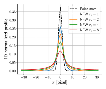
Figure 2: The normalized one-dimensional ($1$D) profiles of smoothed basis atoms, which are slices of the corresponding $2$D profiles (shown in Figure 1) at $y=0$. The scale radii are in pixels.

In order to reconstruct high-resolution, high-S/N mass maps, we incorporate prior information on the density contrast field into the reconstruction by modeling the density field as a sum of basis atoms in a “dictionary”:

$$\delta=\mathbf{\Phi}\cdot x,$$ (2)

where $\mathbf{\Phi}$ is the matrix operator transforming from the projection coefficient vector $x$ to the density contrast field $\delta$. The column vectors of $\mathbf{\Phi}$ are the basis “atoms” of the model dictionary and denoted as $\phi_{s}$.

There have been a few studies that adopt different dictionaries for $3$D weak-lensing map reconstructions: (i) Simon et al. (2009) perform a reconstruction in Fourier space, which is equivalent to representing the density contrast field with sinusoidal functions. However, sinusoidal functions are not localized in configuration space, and the density contrast field is not sparse in Fourier space. Therefore, sparsity priors cannot be directly applied to this model dictionary for high-resolution mass map reconstructions. (ii) Leonard et al. (2014) model the density contrast field with starlets (Starck et al., 2015). However, the starlet dictionary does not account for the angular scale difference at different lens redshifts, and is not specifically designed to model the clumpy mass distribution in the universe. It is worth exploring other dictionaries for our purpose of weak-lensing mass reconstruction.

In the standard cosmological model, dark matter is concentrated in roughly spherical “halos”, which have the NFW density profile (Navarro et al., 1997). Motivated by this fact, we generate a model dictionary using NFW atoms with $N$ typical scale radii $r_{s}~{}(s=1,...,N)$ in comoving coordinates. An atom has the NFW surface density profile on the transverse plane (Takada & Jain, 2003) and the Dirac $\delta$ function in the line of sight direction. Following Leonard et al. (2014), we neglect the size of halos along the line of sight since the resolution scale of the reconstruction is much larger than the halos.

The multiscale NFW atom is defined as

$$\phi_{s}(\vec{r}_{\theta},z)=\frac{f}{2\pi r_{s}^{2}}\,F(|\vec{r}_{\theta}|/r_{s})\,\delta_{D}(z),$$ (3)

where $\vec{r}_{\theta}$ is the projection of the comoving position on the transverse plane,

$$F(x)=\begin{cases}-\frac{\sqrt{c^{2}-x^{2}}}{(1-x^{2})(1+c)}+\frac{\operatorname{arccosh}\left(\frac{x^{2}+c}{x(1+c)}\right)}{(1-x^{2})^{3/2}}&(x<1),\\ \frac{\sqrt{c^{2}-1}}{3(1+c)}(1+\frac{1}{c+1})&(x=1),\\ -\frac{\sqrt{c^{2}-x^{2}}}{(1-x^{2})(1+c)}+\frac{\arccos\left(\frac{x^{2}+c}{x(1+c)}\right)}{(x^{2}-1)^{3/2}}&(1<x\leq c),\\ 0&(x>c)\,.\end{cases}$$ (4)

$f=1/[\ln(1+c)-c/(1+c)]$, and $c$ is the halo concentration. For simplicity, we fix $c=4$ for the NFW atoms in our dictionary. In the present paper, we adopt a hard truncation on the NFW profile at a radius equals $cr_{s}$. Studying the influence of different truncation forms (Oguri & Hamana, 2011) on the mass map reconstruction is left to our future work.

Compared to other model dictionaries, our NFW dictionary is motivated by a physical consideration on the clumpy mass distribution in the universe. Furthermore, the multiscale NFW atoms are set up in comoving coordinates, with an account of the scale difference in the angular coordinates for halos at different lens redshifts. The corresponding NFW atom in the angular separation coordinates is

$$\begin{split}\phi_{s}(\vec{\theta},z)=\frac{f\chi^{2}(z)}{2\pi r_{s}^{2}}\,F(|\vec{\theta}|\chi(z)/r_{s})\,\delta_{D}(z),\end{split}$$ (5)

where $\chi(z)$ is the comoving distance to redshift $z$.

For the NFW dictionary, the transform from the projection coefficient vector to the density contrast field of Equation (2) is written as

$$\delta(\vec{r})=\sum_{s=1}^{N}\int d^{3}r^{\prime}\phi_{s}(\vec{r}-\vec{r^{\prime}})x_{s}(\vec{r^{\prime}})\,.$$ (6)

To simplify the notation, we compress the projection coefficient vectors on the basis atoms with multiple scales into a single column vector:

$$x=\begin{pmatrix}x_{0}\\ x_{1}\\ ...\\ x_{N}\end{pmatrix},$$ (7)

and write the dictionary transform operator into a row vector:

$$\mathbf{\Phi}=\begin{pmatrix}\int{\rm d}^{3}r\,\phi_{0}(\vec{r})~{}\int{\rm d}^{3}r\,\phi_{1}(\vec{r})~{}...~{}\int{\rm d}^{3}r\,\phi_{N}(\vec{r})\end{pmatrix}.$$ (8)

For an additional test and comparison, we also construct a dictionary with the point-mass atoms which are represented by the $3$D Dirac function as

$$\phi_{\rm{PM}}(\vec{\theta},z)=\delta_{\rm D}(\theta_{1})\,\,\delta_{\rm D}(\theta_{2})\,\,\delta_{\rm D}(z)\,.$$ (9)

The $2$D profiles of the NFW atoms and the point-mass atom on the transverse plane are shown in Figure 1. The corresponding $1$D profiles are plotted in Figure 2. The profiles are smoothed with a Gaussian kernel and pixelized on linearly spaced grids. Details on the smoothing and pixelizing operations are described in Section 2.3.2.

We define the forward transform operator $\mathbf{A}=\mathbf{P}\cdot\mathbf{Q}\cdot\mathbf{\Phi}$ where $\mathbf{P}$ represents systematic effects and $\mathbf{Q}$ represents the physical lensing effect. With Equations (1) and (2), we write the transform from the coefficient vector $x$ to the observed lensing shear field as

$$\gamma=\mathbf{A}\cdot x+\epsilon\,.$$ (10)

2.2 Weak gravitational lensing

Figure 3: Top panel: Normalized lensing kernels as a function of source redshift with lens redshifts fixed. The solid lines are the kernels for the source galaxies with precise spectroscopic redshifts, whereas the dashed lines are for source redshifts with HSC-like photometric redshift errors. Bottom panel: Correlation matrix between the lensing kernels of different lens redshifts. We normalize the diagonal terms to $1\,$. The color map is the correlation matrix for spectroscopic redshift. We also compare the result for the lensing kernel of spectroscopic (photometric) redshift by solid (dashed) contours at levels $0.7$, $0.85$, and $0.98\,$.

The lensing transform operator can be expressed as

$$\mathbf{Q}=\int_{0}^{z_{s}}dz_{l}\,K(z_{l},z_{s})\int d^{2}\theta^{\prime}\,D(\vec{\theta}-\vec{\theta^{\prime}})\,.$$ (11)

$K(z_{l},z_{s})$ is the lensing kernel between lens redshift $z_{l}$ and source redshift $z_{s}$ (Bartelmann & Schneider, 2001), which is given by

$$K(z_{l},z_{s})=\begin{cases}\frac{3H_{0}\Omega_{\rm m}}{2c}\frac{\chi_{l}\chi_{sl}(1+z_{l})}{\chi_{s}E\left(z_{l}\right)}&(z_{s}>z_{l}),\\ 0&(z_{s}\leq z_{l}),\end{cases}$$ (12)

where $E(z)$ is the Hubble parameter as a function of redshift, in units of $H_{0}$.

$$D(\vec{\theta})=-\frac{1}{\pi}(\theta_{1}-i\theta_{2})^{-2}$$ (13)

is the Kaiser-Squares kernel (Kaiser & Squires, 1993), which decays proportional to the inverse-square of the distance. Here $\theta_{1,2}$ are the two components of the angular position vector $\vec{\theta}$.

The top panel of Figure 3 shows the lensing kernels as a function of source redshift for lenses at different lens redshifts. The bottom panel of Figure 3 shows the correlation between the lensing kernels. Each lensing kernel is highly nonlocal, and the lensing kernels of different lens redshifts are strongly correlated as can be seen in the bottom panel. These inherent properties of the lensing kernels result in strong correlation between the column vectors that constitute the forward transform matrix $\mathbf{A}$. As will be discussed in Section 2.4, the strong correlation makes it challenging to reconstruct mass maps with high-resolution in the line of sight direction.

2.3 Systematics

Shear measurement deviates from the true, physical shear owing to a variety of systematic effects in real observations. In this section, we discuss the influence of several major systematics on the lensing shear measurement, and describe the corresponding transform operator by decomposing into three parts of $\mathbf{R}$ (photometric redshift uncertainties), $\mathbf{W}$ (smoothing), and $\mathbf{M}$ (masking).

2.3.1 Photometric redshift Uncertainty

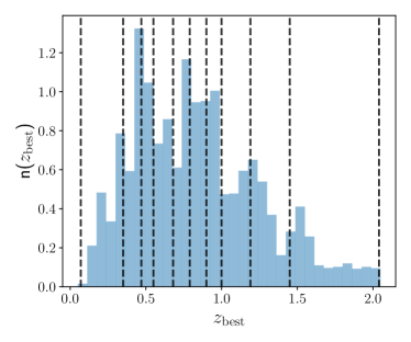
Figure 4: The blue histogram shows the normalized number distribution of the best-fit photo-$z$ (MLZ) estimates from tract $9347$ of the first-year HSC data. We use an equal-number binning scheme to divide the source galaxies into a total of $10$ redshift bins that are indicated by the vertical dashed lines.

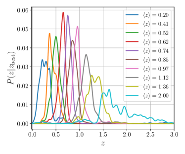
Figure 5: The average PDF of MLZ in $10$ source redshift bins with boundaries defined by the vertical dashed lines in Figure 4.

Photometric redshifts (photo-$z$) are estimated with a limited number of broad optical and near-infrared bands in the current generation weak-lensing surveys. For example, $9$ bands are used for KIDS$+$VIKING survey (Hildebrandt et al., 2020), $5$ bands for DES survey and HSC survey. Unlike the high-precision spectroscopic redshift (spect-$z$) estimation, the photo-$z$ estimation suffers from considerable statistical uncertainties.

Figure 4 shows the histogram of the best-fit estimates of the Machine Learning for photo-Z (MLZ; Carrasco Kind & Brunner, 2013) algorithm for galaxies in tract $9347$ from the photo-$z$ catalog (Tanaka et al., 2018) of the first-year HSC data release (Aihara et al., 2018). The galaxies are divided into ten bins according to the photo-$z$ best-fit estimates. Figure 5 shows the average probability density function (PDF) for galaxies in each redshift bin.

In the presence of photo-$z$ uncertainties, a source galaxy with a best-fit photo-$z$ estimate $z_{s}$ has a posterior probability $P(z|z_{s})$ of being actually located at redshift $z$. This means that there is a possibility $P(z|z_{s})$ that the galaxy image is actually distorted by the shear at redshift $z$. Therefore, the photo-$z$ uncertainty smears the lensing kernel statistically, which we model by a smearing operator

$$\mathbf{R}=\int dzP(z|z_{s})\,.$$ (14)

Figure 3 shows the lensing kernels and their correlations for source redshifts with photo-$z$ uncertainties demonstrated in Figure 5. Compared to the lensing kernels of spect-$z$ that converge to zero at source redshifts lower than the lens redshift, the lensing kernels of photo-$z$ do not converge to zero at the low source redshifts. This is simply because the galaxies with photo-$z$ estimated lower than the lens redshifts may actually be located at higher redshifts. In addition, the photo-$z$ uncertainty only slightly increases the correlations between lensing kernels at different lens plane.

2.3.2 Smoothing

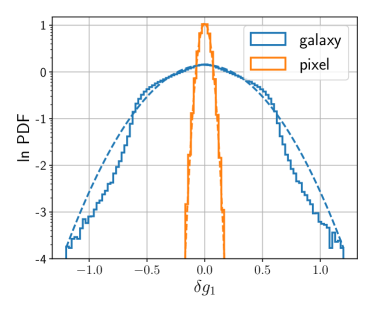
Figure 6: The solid blue (orange) line shows the histogram of the HSC-like shear measurement error on the first component of shear $g_{1}$ on individual galaxy (pixel) level. The dashed lines are the best-fit Gaussian distributions to the corresponding histograms.

The source galaxies are not uniformly distributed in the sky, with substantial fluctuations in the number density. We first smooth the lensing shear measurements, and pixelize the smoothed shear field onto a regular grid. After these procedures, the fast Fourier transform (FFT) can be directly conducted on the transverse plane in each redshift bin to compute the convolution operation in Equation (1). Another benefit of smoothing is that it reduces bias arising from the aliasing effect in the pixelization process since the smoothing kernel reduces the amplitude of the shear signal at high frequency.

We convolve the lensing shear measured from galaxy images with a $3$D smoothing kernel $W(\vec{\theta},z)$. The expectation of the lensing shear field after smoothing is

$$\gamma_{\rm{sm}}(\vec{\theta},z)=\frac{\sum_{i}W(\vec{\theta}-\vec{{\theta}}_{i},z-z_{i})\gamma_{L}(\vec{\theta}_{i},z_{i})}{\sum_{i}W(\vec{\theta}-\vec{{\theta}}_{i},z-z_{i})},$$ (15)

where $z_{i}$ and $\theta_{i}$ refer to the photometric redshift, and transverse position of the $i$th galaxy in the galaxy sample, respectively. $\gamma_{L}$ refers to the shear field before the smoothing.

The smoothing kernel $W(\vec{\theta},z)$ can be decomposed into a transverse component $W_{t}(\vec{\theta})$ and a line of sight component $W_{l}(z)$ as

$$W(\vec{\theta},z)=W_{t}(\vec{\theta})\,W_{l}(z)\,.$$ (16)

We use an isotropic $2$D Gaussian kernel and a $1$D top-hat kernel to smooth the shear field in the transverse plane and in the line of sight direction, respectively. These components are given by

$$\begin{split}W_{t}(\vec{\theta})&=\frac{1}{2\pi\beta^{2}}\exp(-\frac{|\vec{\theta}|}{2\beta^{2}}),\\ W_{l}(z)&=\begin{cases}1/\Delta z&(|z|<\Delta z/2),\\ 0&{\rm othewise},\end{cases}\end{split}$$ (17)

where we set $\beta=1.5$ arcmin in this paper. By definition, the smoothing kernel is normalized as

$$\int{\rm d}^{3}r\,W(\vec{r})=1\,.$$ (18)

Assuming that the galaxy number distribution varies slowly at the smoothing scale, the smoothed shear can be written into

$$\gamma_{\rm{sm}}=\mathbf{W}\cdot\gamma_{L},$$ (19)

where $\mathbf{W}$ is the smoothing operator defined as

$$\mathbf{W}=\int{\rm d}^{3}r^{\prime}\,W(\vec{r}-\vec{r^{\prime}})\,.$$ (20)

We note that another widely used scheme is to average the shear measurements in each pixel. Such a scenario is equivalent to resampling the shear field smoothed with a $3$D top-hat kernel with the same scale as the pixels.

After smoothing, we pixelize the shear field on $N_{x}\times N_{y}\times N_{z}$ grids, where $N_{x}$ and $N_{y}$ are the number of pixels of the two orthogonal axes of the transverse plane, and $N_{z}$ is the number of pixels in the line of sight direction. We denote by $\gamma_{\alpha}$ the smoothed shear measurements recorded on the pixel with index $\alpha$, where $1\leq\alpha\leq N_{x}\times N_{y}\times N_{z}$. The grids on the transverse planes are equally spaced with a pixel size of $1\arcmin$. In the line of sight direction, we set binning with equal galaxy number as shown in Figure 4.

Similarly, we pixelize the projection coefficient vector $x$ onto an $N_{x}\times N_{y}\times N_{l}$ grid. In this paper, the projection coefficient vector is pixelized in equal spacing ranging from redshift $0.01$ to redshift $0.85$. Here, we use $N_{l}$ to denote the number of the lens planes and $x_{\beta}$ to denote the projection field element with index $1\leq\beta\leq N_{x}\times N_{y}\times N_{l}\times N$, where the last $N$ is the number of NFW dictionary frames representing different physical scale radii. The corresponding pixelized elements of the forward transform matrix $\mathbf{A}$ is denoted as $A_{\alpha\beta}$.

In order to see the effect of smoothing clearly, we plot the histograms of the statistical shear measurement errors due to shape noise and sky variance for the galaxies in tract $9347$ of the first-year HSC shear catalog (Mandelbaum et al., 2018). In Figure 6, we compare the error on an individual galaxy basis and that of individual pixels after the smoothing and pixelization procedures described in this section. The standard deviation of the individual pixel errors is much smaller than for the galaxies owing to the smoothing. We also note that, even though the shear measurement error for the galaxies does not follow a Gaussian distribution, the error after smoothing and pixelization is well described by a Gaussian distribution, which is simply explained by the central limit theorem.

2.3.3 Masking

In real observations, shear measurements can be performed in a finite region of the sky, and the boundaries often have complicated geometries. Moreover, many isolated sub-regions near the bright stars are masked out.

We define the masking window function as

$$M(\vec{r})=\begin{cases}1&n_{\rm{sm}}\geq 1,\\ 0&\rm{otherwise},\end{cases}$$ (21)

where $n_{\rm{sm}}$ is the smoothed galaxy number density. We define the masking operator as

$$\mathbf{M}=\int{\rm d}^{3}r^{\prime}\,M(\vec{r^{\prime}})\delta_{D}(\vec{r}-\vec{r^{\prime}}),$$ (22)

where $\delta_{D}(\vec{r})$ is $3$D Dirac delta function.

Taking into account the systematics discussed in previous Sections 2.3.1–2.3.3, the systematic operator is

$$\mathbf{P}=\mathbf{M}\cdot\mathbf{W}\cdot\mathbf{R}\,.$$ (23)

2.4 Density map reconstruction

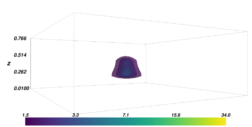
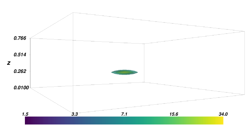
Figure 7: The density map reconstruction with LASSO (left) and with our adaptive LASSO (right) algorithm. The $z$-axes are for redshift. The mass of halo is $M_{200}=10^{15}~{}\text{h}^{-1}M_{\odot}$, and its redshift is $z=0.35$. The color bars indicate the values of reconstructed density contrast. Note that our adaptive LASSO mitigates elongation in the $z$-direction (along line of sight) and suppresses the shrinkage in LASSO, and thus the reconstructed density values are large, compared to the LASSO result shown in the left. Shear measurement errors and photo-$z$ uncertainties are not considered in this test simulation.

The projection coefficients can be estimated by optimizing a penalized loss function. An estimator is generally defined as

$$\hat{x}=\mathop{\rm arg~{}min}\limits_{x}\left\{\frac{1}{2}{}_{\Sigma}\mathinner{\!\left\lVert(\gamma-\mathbf{A}x)\right\rVert}_{2}^{2}+\lambda C(x)\right\},$$ (24)

where ${}_{\Sigma}\mathinner{\!\left\lVert(\gamma-\mathbf{A}x)\right\rVert}_{2}^{2}$ is the $l^{2}$ norm of residuals weighted by the inverse of the covariance matrix $\Sigma$ of the shear measurement error, which measures the difference between the prediction and the data. $C(x)$ is the penalty term measuring the deviation of the coefficient estimate $x$ from the prior assumption. The estimation with the “penalty” term prefers parameters that are able to describe the observation with a specified prior information. The penalty parameter $\lambda$ adjusts the relative weight between the data and the prior assumption in the optimization process.

There have been a few studies that adopt different penalties for $3$D weak-lensing map reconstructions: (i) Simon et al. (2009) propose to use the Wiener filter, which is also known as $l^{2}$ ridge penalty ($C=\mathinner{\!\left\lVert x\right\rVert}^{2}_{2}$), to find a penalized solution in Fourier space. Oguri et al. (2018) apply the method of Simon et al. (2009) to the first-year data of the Hyper Suprime-Cam Survey (Aihara et al., 2018). It is found that the density maps reconstructed by the method suffer from significant line of sight smearing with standard deviation of $\sigma_{z}=0.2-0.3$. (ii) Leonard et al. (2014) use GLIMPSE algorithm, which adopts a derivative version of the $l^{1}$ LASSO penalty ($C=\mathinner{\!\left\lVert x\right\rVert}^{1}_{1}$) to find a sparse solution in the starlet dictionary (Starck et al., 2015). GLIMPSE reduces the smearing by adopting a “greedy” coordinate descent algorithm that forces the structure to grow only on the most related lens redshift plane.

In this paper, we use another derivative version of the LASSO penalty – the adaptive LASSO penalty. We first normalize the column vectors of the forward transform matrix in Section 2.5. We then introduce the loss function with the adaptive LASSO penalty in Section 2.5.1. Finally, we find the minimum of the loss function in Section 2.5.2 with the FISTA algorithm (Beck & Teboulle, 2009).

2.5 Normalization

The $l^{2}$ norm of the $i$th column vector of $\mathbf{A}$ weighted by the inverse of the noise covariance matrix is defined as

$$\mathcal{N}_{i}=(\Sigma^{-1})_{\alpha\beta}A_{i\alpha}A_{i\beta}\,.$$ (25)

The column vectors have different weighted $l^{2}$ norms. Since the gradient descent algorithm, which will be used to solve Equation (24) in Section 2.5.2, takes each column vector equally, we normalize the column vectors before performing the density map reconstruction to boost the convergence speed of the gradient descent iteration. The normalized forward transform matrix and projection parameters are given by

$$\begin{split}A^{\prime}_{\alpha\beta}&=A_{\alpha\beta}/\mathcal{N}_{\alpha}^{\frac{1}{2}},\\ x^{\prime}_{\beta}&=x_{\beta}\mathcal{N}_{\beta}^{\frac{1}{2}}\,.\end{split}$$ (26)

2.5.1 Adaptive LASSO

The LASSO algorithm uses $l^{1}$ norm of the projection coefficient vector to regularize the modeling. The estimator is defined as

$$\hat{x^{\prime}}^{\rm{LASSO}}=\mathop{\rm arg~{}min}\limits_{x}\left\{\frac{1}{2}{}_{\Sigma}\mathinner{\!\left\lVert(\gamma-\mathbf{A^{\prime}}\cdot x^{\prime})\right\rVert}_{2}^{2}+\lambda\mathinner{\!\left\lVert x^{\prime}\right\rVert}^{1}_{1}\right\},$$ (27)

where $\mathinner{\!\left\lVert\mathchoice{\mathbin{\vbox{\hbox{\scalebox{0.5}{$\displaystyle\bullet$}}}}}{\mathbin{\vbox{\hbox{\scalebox{0.5}{$\textstyle\bullet$}}}}}{\mathbin{\vbox{\hbox{\scalebox{0.5}{$\scriptstyle\bullet$}}}}}{\mathbin{\vbox{\hbox{\scalebox{0.5}{$\scriptscriptstyle\bullet$}}}}}\right\rVert}_{1}^{1}$ and $\mathinner{\!\left\lVert\mathchoice{\mathbin{\vbox{\hbox{\scalebox{0.5}{$\displaystyle\bullet$}}}}}{\mathbin{\vbox{\hbox{\scalebox{0.5}{$\textstyle\bullet$}}}}}{\mathbin{\vbox{\hbox{\scalebox{0.5}{$\scriptstyle\bullet$}}}}}{\mathbin{\vbox{\hbox{\scalebox{0.5}{$\scriptscriptstyle\bullet$}}}}}\right\rVert}_{2}^{2}$ refer to the $l^{1}$ norm and $l^{2}$ norm, respectively, and $\lambda$ is the penalty parameter for the LASSO estimation.

The LASSO algorithm searches and selects the parameters that are relevant to the measurements, and simultaneously estimates the values of the selected parameters. It has been shown by Zou (2006) that when the column vectors of the forward transform matrix $\mathbf{A^{\prime}}$ are highly correlated, the algorithm cannot select the relevant atoms from the dictionary consistently. In addition, the estimated parameters are often biased owing to the shrinkage in the LASSO regression. We note that, for the density map reconstruction problem here, the column vectors are highly correlated even in the absence of photo-$z$ uncertainties since the lensing kernels for lenses at different redshifts overlap significantly, i.e. highly correlated as shown in Figure 3. Therefore, the LASSO algorithm cannot precisely determine the consistent mass distribution in redshift, and the reconstructed map suffers from smearing in the line of sight direction even in the absence of noises.

Figure 7 shows an example reconstruction results for a single halo with mass $M_{200}=10^{15}~{}\text{h}^{-1}M_{\odot}$ at redshift $0.35$. The shear measurement and photo-$z$ uncertainties are not included in this simulation. We find significant smearing of the mass distribution with the LASSO algorithm (left panel of Figure 7).

To overcome the problem, Zou (2006) proposes the adaptive LASSO algorithm, which uses adaptive weights to penalize different projection coefficients in the $l^{1}$ penalty. The adaptive LASSO algorithm performs a two-step process. In the first step, the standard (nonadaptive) LASSO is used to estimate the parameters. Let us denote the preliminary estimation as $\hat{x^{\prime}}_{\rm{LASSO}}$. In the second step, the preliminary estimate is used to calculate the nonnegative weight vector for penalization as

$$\hat{w}=\frac{1}{\mathinner{\!\left\lvert\hat{x^{\prime}}_{\rm{LASSO}}\right\rvert}^{\tau}},$$ (28)

where we set the hyperparameter $\tau$ to $2\,$. The adaptive LASSO estimator is then given by

$$\hat{x^{\prime}}=\mathop{\rm arg~{}min}\limits_{x^{\prime}}\left\{\frac{1}{2}{}_{\Sigma}\mathinner{\!\left\lVert(\gamma-\mathbf{A^{\prime}}\cdot x^{\prime})\right\rVert}^{2}_{2}+\lambda_{\rm{ada}}\mathinner{\!\left\lVert\hat{w}\circ x^{\prime}\right\rVert}^{1}_{1}\right\},$$ (29)

where “$\circ$” refers to the element-wise product. $\lambda_{\rm{ada}}$ is the penalty parameter for the adaptive LASSO, which does not need to be the same as the penalty parameter for the preliminary LASSO estimation $\lambda$. The adaptive weights enhance the shrinkage in the soft thresholding for the coefficients with smaller amplitudes, whereas the weights suppress the shrinkage for the coefficients with larger amplitudes.

To simplify the equations in the following, we rewrite the loss function with the Einstein notation as

$$\begin{split}L(x^{\prime})&=\frac{1}{2}(\Sigma^{-1})_{\alpha\beta}(\gamma^{*}_{\alpha}-A^{\prime*}_{\alpha i}x^{\prime}_{i})(\gamma_{\beta}-A^{\prime}_{\beta j}x^{\prime}_{j})\\ &+\lambda_{\rm{ada}}\hat{w_{\beta}}\mathinner{\!\left\lvert x^{\prime}_{\beta}\right\rvert},\end{split}$$ (30)

and the quadruple term in the loss function as

$$G(x^{\prime})=\frac{1}{2}\Sigma^{-1}_{\alpha\beta}(\gamma^{*}_{\alpha}-A^{\prime*}_{\alpha i}x^{\prime}_{i})(\gamma_{\beta}-A^{\prime}_{\beta j}x^{\prime}_{j})\,.$$ (31)

2.5.2 FISTA

Beck & Teboulle (2009) propose the Fast Iterative Soft Thresholding Algorithm (FISTA) to solve the LASSO problem. Since the loss functions of the LASSO and the adaptive LASSO differ only in their penalty terms, FISTA is also applicable to solve the adaptive LASSO problem in a straightforward manner. In this paper, we apply FISTA to solve both the preliminary LASSO estimation and the adaptive LASSO estimation.

We first explain the LASSO preliminary estimation. The coefficients are initialized as $x_{i}^{(1)}=0$. According to FISTA, we iteratively update the projection coefficient vector $x$. Taking the $n$th iteration as an example, a temporary update is first calculated as

$$x^{\prime(n+1)}_{i}=\mathrm{ST}_{\lambda}\left(x^{\prime(n)}_{i}-\mu\partial_{i}G(x^{\prime(n)})\right),$$ (32)

where $\mathrm{ST}$ is the soft thresholding function defined as

$$\mathrm{ST}_{\lambda}\left(x^{\prime}\right)=\mathrm{sign}(x^{\prime})\max\left\{\mathinner{\!\left\lvert x^{\prime}\right\rvert}-\lambda,0\right\}\,.$$ (33)

The soft thresholding is a part of the LASSO algorithm, which selects the modes with amplitude greater than $\lambda$, and shrinks the selected estimation by $\lambda$. The coefficient $\mu$ is the step size of the gradient descent iteration, and $\partial_{i}G(x^{\prime(n)})$ is the $i$th element of the gradient vector of $G$ at point $x^{\prime(n)}$:

$$\partial_{i}G(x^{\prime(n)})=\Sigma^{-1}_{\alpha\beta}\real\left\{A^{\prime*}_{\alpha i}(\gamma_{\beta}-A^{\prime}_{\beta j}x^{\prime}_{j})\right\},$$ (34)

where $\real\left\{\bullet\right\}$ returns the real part of the input vector. FISTA requires an additional update using a weighted average between $x^{\prime(n+1)}$ and $x^{\prime(n)}$ as

$$\begin{split}t^{(n+1)}&=\frac{1+\sqrt{1+4(t^{(n)})^{2}}}{2},\\ x^{\prime(n+1)}&\leftarrow x^{\prime(x+1)}+\frac{t^{(n)}-1}{t^{(n+1)}}(x^{\prime(n+1)}-x^{\prime(n)}),\end{split}$$ (35)

where the relative weight is initialized as $t^{(1)}=1$.

FISTA converges as long as the gradient descent step size $\mu$ satisfies

$$0<\mu<\frac{1}{\mathinner{\!\left\lVert\mathbf{A^{\dagger}}\cdot\mathbf{\Sigma}^{-1}\cdot\mathbf{A}\right\rVert}},$$ (36)

where the operation $\mathinner{\!\left\lVert\bullet\right\rVert}$ returns the spectrum norm of the input matrix. The spectral norm is estimated by simulating a large number of random vectors with $l^{2}$ norms equal one with different realizations. The matrix operator $\mathbf{A^{\dagger}}\cdot\mathbf{\Sigma}^{-1}\cdot\mathbf{A}$ is subsequently applied to each random vector to yield a corresponding transformed vector. The spectral norm is determined as the maximum $l^{2}$ norm of the transformed vectors.

As summarized in the below, we first initialize the projection coefficients as zero, and use FISTA to find the global minimum of the LASSO loss function. Thus-obtained global minimum is the preliminary one. We then use the preliminary LASSO estimation to weight the coefficients and calculate the adaptive LASSO loss function. Finally, we set the preliminary LASSO estimation as the “warm” start of the adaptive LASSO estimation, and FISTA again to find the global minimum of the adaptive LASSO loss function, which is our final solution.

Algorithm Our Algorithm

1:$\gamma$: Pixelized complex $3$D shear field

2:$\delta$: $3$D array of density contrast

3:Normalize column vectors of $\mathbf{A}$

4:Estimate step size $\mu$ and $\mathbf{\Sigma}$

5:Initialization:

6:$x^{\prime(1)}=0$

7:$\hat{w}=1$

8:$t^{(1)}=1$,$i=1$, $j=1$

9:while $j\leq 2$ do

10:   while $i\leq N_{\rm{iter}}$ do

11:      # soft thresholding

12:      $x^{\prime(n+1)}_{i}=\mathrm{ST}_{\hat{w}\lambda}\left(x^{\prime(n)}_{i}-\mu\partial_{i}G(x^{\prime(n)})\right)$

13:      # FISTA algorithm

14:      $t^{(n+1)}=\frac{1+\sqrt{1+4(t^{(n)})^{2}}}{2}$

15:      $x^{\prime(n+1)}\leftarrow x^{\prime(x+1)}+\frac{t^{(n)}-1}{t^{(n+1)}}(x^{\prime(n+1)}-x^{\prime(n)})$

16:      $i=i+1$

17:   end while

18:   Re-initialization:

19:   $\hat{w}=\mathinner{\!\left\lvert\hat{x^{\prime}}_{\rm{LASSO}}\right\rvert}^{-2}$, $\lambda\leftarrow\lambda_{\rm{ada}}$

20:   $\hat{x^{\prime}}^{(1)}=x^{\prime(N_{\rm{iter}})}$

21:   $t^{(1)}=1$, $i=1$

22:   $j=j+1$

23:end while

24:$\delta=\mathbf{\Phi}\mathcal{N}^{-\frac{1}{2}}x^{\prime(N_{\rm{iter}})}$

3 Cluster Detection

We simulate weak-lensing shear induced by NFW halos with various masses and redshifts. The generated shear fields are used to distort the HSC mock galaxy shapes with different realizations of shear measurement and photo-$z$ uncertainties (Section 3.1).

We then test our algorithm using the mock catalogs with varying the penalty parameter in our model (Section 3.2). We also compare our method that uses the NFW dictionary with one using the point mass dictionary (Section 3.3).

3.1 Simulations

We use halos with a variety of masses and redshifts in the range $10^{14}\text{h}^{-1}M_{\odot}<M<10^{15}\text{h}^{-1}M_{\odot}$, and $0.05<z<0.85$, respectively. We divide the parameter space into eight redshift bins and eight mass bins with equal separation. We randomly shift the input halo redshift and halo mass from the bin center by a small amount in order to avoid repeatedly sampling at the exact same halo mass and redshift.

The concentration parameter $c_{\rm h}$ of a NFW halo is determined as a function of the halo mass ($M_{200}$) and redshift ($z_{\rm h}$) according to Ragagnin et al. (2019):

$$c_{\rm h}=6.02\times\left(\frac{M_{200}}{10^{13}M_{\odot}}\right)^{-0.12}\left(\frac{1.47}{1.+z_{\rm h}}\right)^{0.16}\,.$$ (37)

The weak-lensing shear fields of the NFW halos are calculated according to Takada & Jain (2003). The shear distortions are applied to one hundred realizations of galaxy catalogs with the HSC-like shear measurement error and photo-$z$ uncertainty.

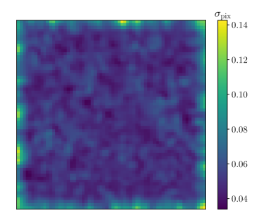
Figure 8: The standard deviation pixel map of the HSC-like shear measurement error for the fifth source galaxy bin ($0.69\leq z<0.80$).

The mock galaxy catalogs are generated using the HSC S16A shear catalog (Mandelbaum et al., 2018). We use the galaxies in a 1 square degree field at the center of tract 9347 (Aihara et al., 2018). The average galaxy number density in this region is $22.94~{}\rm{arcmin}^{-2}$. The positions of galaxies are randomized to distribute homogeneously in the one-square degree stamp. We randomly assign redshift for each galaxy following the MLZ photo-$z$ probability distribution function (Tanaka et al., 2018).

We simulate the HSC-like shear measurement error due to shape noise and sky variance with different realizations by randomly rotating the galaxies in the shear catalog. The shear measurement error on individual galaxy level and individual pixel level are demonstrated in Figure 6. The standard deviation map of the noise is demonstrated in Figure 8.

3.2 NFW atoms

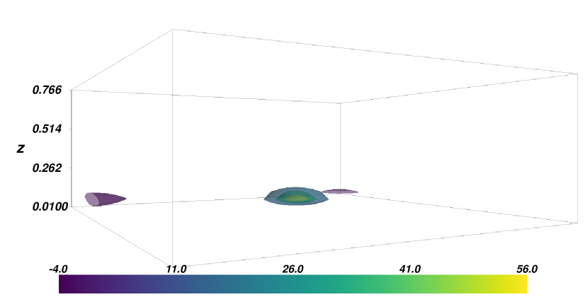
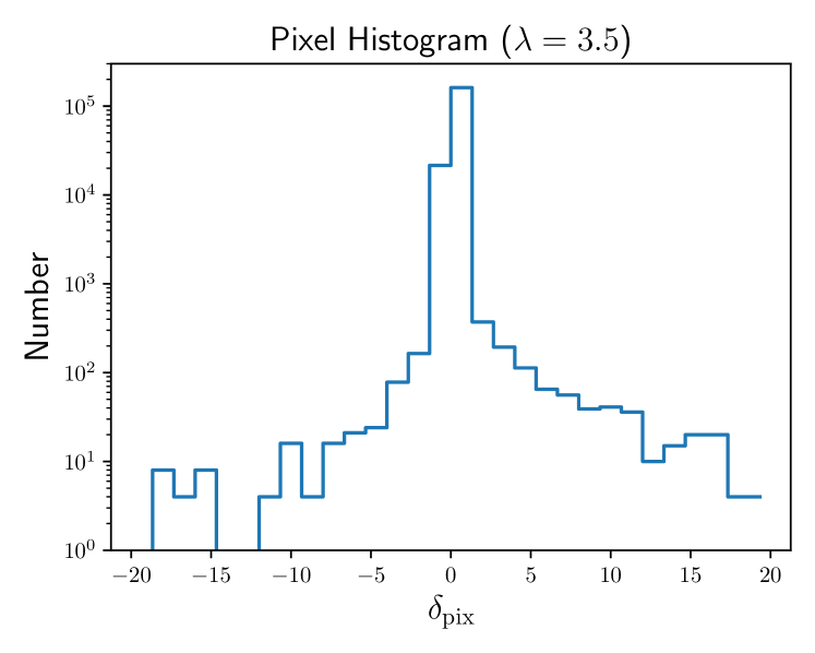
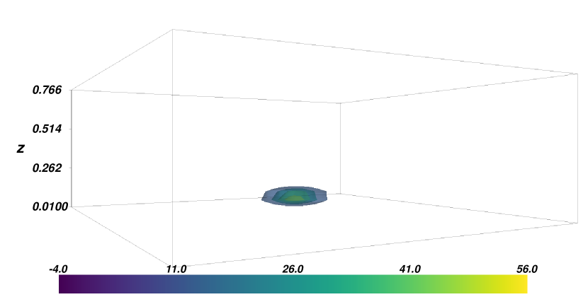
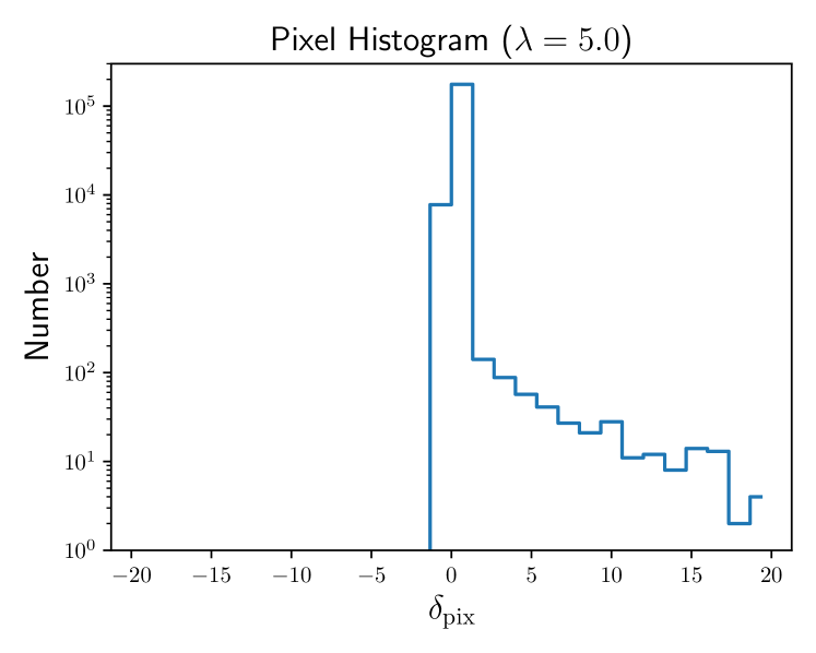
Figure 9: The upper panels show the density maps reconstructed from a mock galaxy shear catalog, which includes shear measurement and photo-$z$ uncertainties, using our algorithm with penalty parameters $\lambda=3.5$ (left) and $\lambda=5.0$ (right). The axes and color maps have the same meanings as Figure 7. The lower panels show the corresponding number histograms of pixel values. The input halo mass is $M_{200}=10^{15.02}~{}\text{h}^{-1}M_{\odot}$, and its redshift is $z=0.164\,$.

In this section, we test the performance of our algorithm by adopting models where the matter density field is represented by multiscale NFW atoms. The dictionary is constructed with three frames of different NFW scale radii in comoving coordinate: $0.12~{}\text{h}^{-1}$ Mpc, $0.24~{}\text{h}^{-1}$ Mpc, and $0.36~{}\text{h}^{-1}$ Mpc. The truncation radii are set to four times the scale radii for the atoms in the dictionary, i.e., we assume $c_{\rm h}=4$. Note that each frame of our dictionary fixes the scale radius in comoving coordinates and thus the NFW atoms have different angular sizes when placed at different redshift.

We test the algorithm with varying the penalty parameter for the LASSO estimation with $\lambda=3.5$, $4.0$, and $5.0$. The corresponding penalty parameters for the final adaptive LASSO estimations are set to $\lambda_{\rm{ad}}=\lambda^{\tau+1}$. Here, both the LASSO estimation and our adaptive LASSO estimation select the pixels with signal-to-noise ratios greater than $\lambda$ in each gradient descent iteration, and the local density is estimated for the selected pixels with a shrinkage of the estimation amplitude. The LASSO estimation shrinks the density amplitudes by $\lambda$ for every selected pixels, whereas the adaptive LASSO estimation suppresses the shrinkage if the preliminary estimation for the pixel is greater than $\lambda$, by down-weighting their penalties, and otherwise it enhances the shrinkage.

We’d like to reconstruct with the resolution limit set by the Gaussian smoothing kernel with a standard deviation of $1\farcm 5$ and the $1\arcmin$ pixel scale as described in Sections 2.3.2. In addition, we smooth the reconstructed density field with the same Gaussian kernel in each lens redshift plane.

Figure 9 shows the $3$D density maps reconstructed with different penalty parameters for a halo with $M_{200}=10^{15.02}~{}\text{h}^{-1}M_{\odot}$ at redshift $0.164$. The corresponding pixel value histograms are shown in Figure 9. Our adaptive LASSO algorithm assigns zero to a fraction of the reconstructed pixels that are mostly noises, while retaining strong signals. The right panels demonstrate a case where almost all of the pixels with pure noise are set to zero when a large penalty parameteris adopted. It is important to note that the reconstructed density maps are not compromised by line of sight smearing, i.e. the reconstructed lens is localized in redshift.

Following Leonard et al. (2014), we normalize the detected peaks in the $l$th ($l=1...20$) lens redshift plane to account for the peak amplitude difference arising from the difference in the norm of the lensing kernels in different redshift bins:

$$\delta^{\rm{n}}_{\rm{peak}}(\vec{\theta},z_{l})=\delta_{\rm{peak}}(\vec{\theta},z_{l})/\mathcal{R}_{l}^{\frac{1}{2}},$$ (38)

where the normalization matrix is defined as

$$\mathcal{R}_{l}=\sum_{s}K^{2}(z_{l},z_{s})\,,$$ (39)

where $K(z_{l},z_{s})$ is the lensing kernel. In Figure 10, we show the histograms of the normalized peaks with different penalty parameters. There, we stack the histograms from $100$ realizations of all the halos sampled in the redshift-mass plane. In addition, we generate $1000$ realizations of pure noise catalogs and perform the reconstruction using the noise catalogs in order to examine the noise properties. The histograms of the normalized peaks detected from the pure noise catalogs are shown in Figure 10 along with the best-fit Gaussian functions of the noise peak histograms.

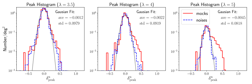
Figure 10: The peak counts as a function of peak overdensity for maps reconstructed with different setups. We plot the peak number density per square-degree. The solid red histograms show the results of the reconstructions from the mock shear catalogs with penalty parameters: $\lambda=3.5,4.0,5.0$, from left to right. The dashed blue histograms are the corresponding results of the reconstruction from $1000$ realizations of pure noise catalogs. The gray lines are the best-fit Gaussian distributions to the noise peak histograms.

We find that the number counts including both true and false peaks decrease as the penalty parameter $\lambda$ increases. In addition, the standard deviation of noise peaks decreases as $\lambda$ increases. As a result, with $\lambda=5.0$, we find a clearer excess in the positive peak counts compared with the noise peak histograms, especially at the high density contrast. This is expected because a higher penalty parameter prefers a sparser solution; more peaks originating from the noise are removed than those from real clusters at the high density contrast.

We demonstrate the position offsets of the detected halos compared to the input positions in Figure 11. The left panel shows the $2$D number histograms stacked over all the simulations as a function of the angular distance and the redshift offsets. We see clear clustering of the peaks close to the position of the input halo on the stacked number histogram. For each simulation, we identify positive peaks closest to the input position (in the pixel unit). If a closest peak is located inside the region denoted with the dashed box in the left panel of Figure 11, we regard it as a “true” peak detection. Other identified peaks, which include both positive and negative peaks, are judged to be false detection.

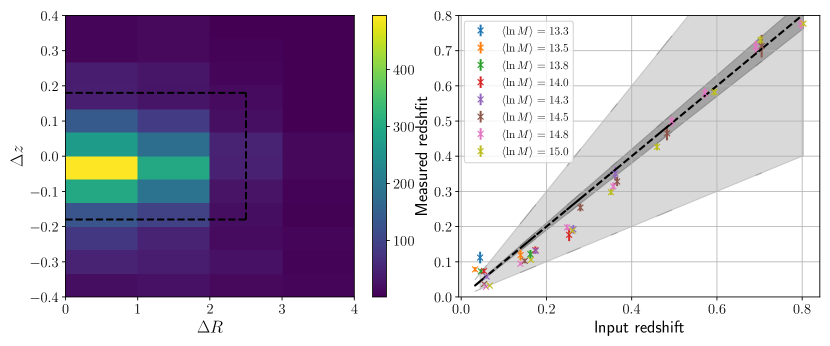
Figure 11: The left panel shows the stacked $2$D distribution of the deviations of detected peak positions from the centers of the corresponding input halos. The $x$-axis is for the deviated distance in the transverse plane, and the $y$-axis is for the deviation in redshift. In each simulation, the positive peak inside the dashed black box with the minimal offset (in the pixel unit) from the position of the input halo is taken as “true” detection. The right panel shows the redshift deviation of detected peaks. The $x$-axis is the input halo redshifts, and the $y$-axis is the redshift of the detected peak. The cross-points denote the average of the detected peaks for each halo over different noise realizations, and the error-bars indicate the uncertainties of the averages. The deep gray area indicates relative redshift bias less than $0.05$, and the light gray area for relative redshift bias less than $0.5$. These results are based on our reconstruction with the NFW dictionary with $\lambda=3.5\,$.

The right panel of Figure 11 shows the estimated redshift of the “true” detections averaged over the simulations (with different noise realizations) for each halo as a function of the input redshift. As shown, the estimated redshifts are slightly lower than the ground truth by $\Delta z\sim 0.03$ for halos in the low-redshift range ($z\leq 0.4$). For halos at $0.4<z\leq 0.85$, the relative redshift bias is below $0.5\%$. The standard deviation of the redshift estimation is $0.092$.

In order to reduce the number of false detections, we select peaks as galaxy clusters if the peak values are greater than an empirically determined threshold. The threshold is set in units of the standard deviation of the noise peaks. We use different detection thresholds ($1.5\sigma$ and $3.0\sigma$) to detect galaxy clusters from the mass maps reconstructed with different penalty parameters. Figures 12 and 13 show the detection rates for halos in the redshift-mass plane for different penalty parameters ($\lambda=3.5$ and $\lambda=5.0$). The corresponding number of false detections per square degree as a function of detection threshold are also demonstrated in the figures.

As shown, the false peak density is successfully reduced for relatively large detection threshold, but the detection rate of halo also decreases. After a few experiments, we have decided to set the detection threshold to $1.5\sigma$ and set the penalty parameter $\lambda$ to $5.0$ since the combination suppresses the false detection to $0.022$ while keeping a high halo detection rate. In summary, our method is able to detect halos with minimal mass of $10^{14.0}\text{h}^{-1}M_{\odot}$, $10^{14.7}\text{h}^{-1}M_{\odot}$, $10^{15.0}\text{h}^{-1}M_{\odot}$ for the low ($z<0.3$), median ($0.3\leq z<0.6$) and high ($0.6\leq z<0.85$) redshift ranges, respectively.

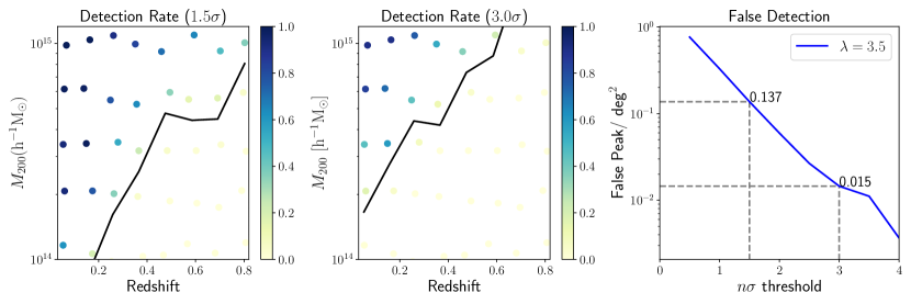
Figure 12: The detection rates and false peak densities for different detection thresholds. The left (middle) panel shows the halo detection rates for detection threshold that equals $1.5\sigma$ ($3.0\sigma$). The black lines indicate the contours for detection rate $0.1\,$. The right panel shows the density of false peaks as a function of detection threshold. The penalty parameter is set to $\lambda=3.5\,$.

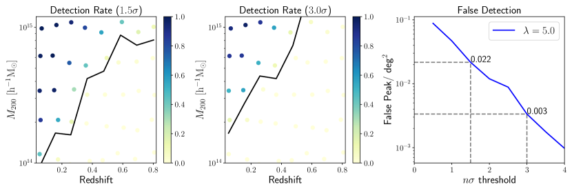
Figure 13: As for Figure 12, but for the penalty parameter $\lambda=5.0\,$.

Using the detection rate measured from our simulations, we are able to predict the number density of detected clusters by assuming the halo mass function of Tinker et al. (2008). We use HMF (Murray et al., 2013), an open-source package, to calculate the halo mass function. The predicted halo detection number density for the setup $\lambda=5$ and $1.5\sigma$ detection threshold is shown in Figure 14. The resulting cluster number density is $0.49$ $\deg^{-2}$, which is much higher than the false detection rate of 0.022 deg^-2. This cluster number density corresponds to $78.4$ clusters for the first-year HSC shear catalog (Mandelbaum et al., 2018) with a survey area of $\sim 160\deg^{2}$. The expected number of detection is slightly higher than the number of $2$D cluster detections ($63$ detected clusters) for the first year HSC shear catalog (Miyazaki et al., 2018b). Furthermore, our $3$D detection method provides an accurate redshift estimation for individual clusters. In contrast, the redshift information is not provided from the $2$D mass map reconstruction.

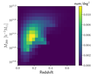
Figure 14: The expected number density of detected clusters per square degree as a function of halo redshift ($x$-axis) and halo mass ($y$-axis). The number density in total is $0.49~{}\deg^{-2}\,$.

3.3 Point mass atoms

We perform an additional test by substituting the default NFW dictionary with point-mass. This test may indicate some certain limitation of our method when applied to a case with very compact (point) objects, which however is unlikely to happen in actual lensing observations.

We set the penalty parameter for the preliminary LASSO to $\lambda=3.5$ and $5.0$. Pramanik & Zhang (2020) propose to incorporate group information into different adaptive LASSO penalty weights by setting the weights for projection coefficients in a group to the average of the adaptive weights in the same group. We assume that the neighboring pixels in the same redshift plane belong to the same structural group (e.g., galaxy cluster and void), and smooth the amplitude of the preliminary LASSO estimation in each lens redshift plane with a top-hat filter of comoving diameter $r_{\rm c}=0.25~{}\text{h}^{-1}$ Mpc. Let us denote the amplitude of the preliminary LASSO estimation with the smoothing as $\mathinner{\!\left\lvert\hat{x}^{\rm{LASSO}}\right\rvert}_{\rm{sm}}$, and adopt the penalty weights given by $\hat{w}=1/\mathinner{\!\left\lvert\hat{x}^{\rm{LASSO}}\right\rvert}_{\rm{sm}}^{\tau}$.

Figure 15 shows the reconstruction result with the point-mass dictionary. Interestingly, several “discrete” masses are assigned to at different redshift bins in the neighboring region of the true halo center. In contrast, as we have seen in Figure 9, the NFW dictionary manages to recover a consistent mass distribution. The problem of the point-mass dictionary originates from the fact that the profile of the point-mass atom in the transverse plane is much more compact than the profile of the input halo, especially when placed at low redshifts.

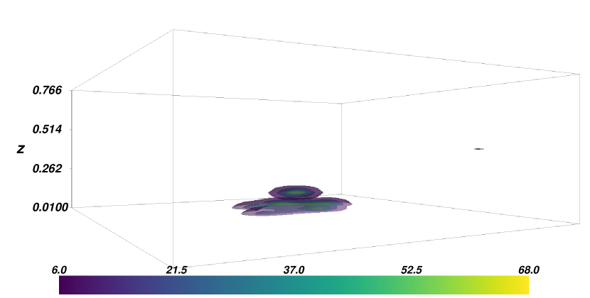
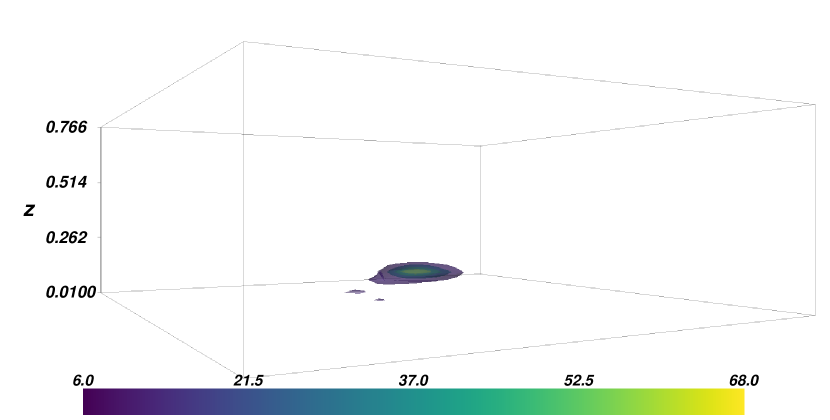
Figure 15: The density maps reconstructed from the mock galaxy shape catalog with the point-mass dictionary. The penalty parameter is $\lambda=3.5$ (left) and $\lambda=5.0$ (right). The axes and color maps have the same meanings as Figure 7. The input halo mass is $M_{200}=10^{15.02}~{}\text{h}^{-1}M_{\odot}$, and its redshift is $z=0.164$.

4 Summary

We have developed a novel method to generate high-resolution $3$D density maps from weak-lensing shear measurement with photometric redshift information. A key improvement over previous similar methods is that we represent a $3$D density field by a collection of NFW atoms with different physical sizes. With a prior assumption that the clumpy mass distribution is sparse in $3$D, we reconstruct the density map using the adaptive LASSO algorithm (Zou, 2006). We show that adopting the standard LASSO algorithm results in significant smearing of structure in the line of sight direction even in the absence of galaxy shape noise and photometric redshift uncertainties. Our adaptive LASSO algorithm efficiently reduces the smearing of structure.

We have examined the performance of cluster detection with the reconstructed $3$D mass maps using mock catalogs that apply shear distortions from isolated halos to galaxies with HSC-like shapes and photo-$z$ uncertainties. Under the realistic conditions, our method is able to detect halo with minimal mass limits of $10^{14.0}\text{h}^{-1}M_{\odot}$, $10^{14.7}\text{h}^{-1}M_{\odot}$, $10^{15.0}\text{h}^{-1}M_{\odot}$ at low ($z<0.3$), median ($0.3\leq z<0.6$) and high ($0.6\leq z<0.85$) redshifts, respectively, with an average false detection of 0.022 deg^-2. The estimated redshifts of the clusters detected in the reconstructed mass maps are slightly lower than the true redshift by $\Delta z\sim 0.03$ for halos at low redshifts ($z\leq 0.4$). The relative redshift bias is below $0.5\%$ for halos at $0.4<z\leq 0.85$, and the standard deviation of the redshift estimation is $0.092$.

We will apply the newly developed $3$D mass map reconstruction technique to the wide-field data from HSC survey (e.g., Mandelbaum et al., 2018; Li et al., 2020) and perform galaxy cluster detection in our future work.

References

- Aihara et al. (2018) Aihara, H., Armstrong, R., Bickerton, S., et al. 2018, PASJ, 70, S8, doi: 10.1093/pasj/psx081
- Bacon & Taylor (2003) Bacon, D. J., & Taylor, A. N. 2003, MNRAS, 344, 1307, doi: 10.1046/j.1365-8711.2003.06922.x
- Bartelmann & Schneider (2001) Bartelmann, M., & Schneider, P. 2001, Physics Reports, 340, 291 , doi: https://doi.org/10.1016/S0370-1573(00)00082-X
- Beck & Teboulle (2009) Beck, A., & Teboulle, M. 2009, SIAM Journal on Imaging Sciences, 2, 183
- Carrasco Kind & Brunner (2013) Carrasco Kind, M., & Brunner, R. J. 2013, MNRAS, 432, 1483, doi: 10.1093/mnras/stt574
- Chang et al. (2018) Chang, C., Pujol, A., Mawdsley, B., et al. 2018, MNRAS, 475, 3165, doi: 10.1093/mnras/stx3363
- de Jong et al. (2013) de Jong, J. T. A., Verdoes Kleijn, G. A., Kuijken, K. H., & Valentijn, E. A. 2013, Experimental Astronomy, 35, 25, doi: 10.1007/s10686-012-9306-1
- Fan et al. (2010) Fan, Z., Shan, H., & Liu, J. 2010, ApJ, 719, 1408, doi: 10.1088/0004-637X/719/2/1408
- Hamana et al. (2020) Hamana, T., Shirasaki, M., & Lin, Y.-T. 2020, PASJ, 72, 78, doi: 10.1093/pasj/psaa068
- Hamana et al. (2004) Hamana, T., Takada, M., & Yoshida, N. 2004, MNRAS, 350, 893, doi: 10.1111/j.1365-2966.2004.07691.x
- Hennawi & Spergel (2005) Hennawi, J. F., & Spergel, D. N. 2005, ApJ, 624, 59, doi: 10.1086/428749
- Hildebrandt et al. (2020) Hildebrandt, H., Köhlinger, F., van den Busch, J. L., et al. 2020, ApJ, 633, A69, doi: 10.1051/0004-6361/201834878
- Hu & Keeton (2002) Hu, W., & Keeton, C. R. 2002, Phys. Rev. D, 66, 063506, doi: 10.1103/PhysRevD.66.063506
- Ivezić et al. (2019) Ivezić, Ž., Kahn, S. M., Tyson, J. A., et al. 2019, ApJ, 873, 111, doi: 10.3847/1538-4357/ab042c
- Jain & Van Waerbeke (2000) Jain, B., & Van Waerbeke, L. 2000, ApJ, 530, L1, doi: 10.1086/312480
- Jeffrey et al. (2018) Jeffrey, N., Abdalla, F. B., Lahav, O., et al. 2018, MNRAS, 479, 2871, doi: 10.1093/mnras/sty1252
- Kaiser & Squires (1993) Kaiser, N., & Squires, G. 1993, ApJ, 404, 441, doi: 10.1086/172297
- Kilbinger (2015) Kilbinger, M. 2015, Reports on Progress in Physics, 78, 086901, doi: 10.1088/0034-4885/78/8/086901
- Lanusse et al. (2016) Lanusse, F., Starck, J. L., Leonard, A., & Pires, S. 2016, ApJ, 591, A2, doi: 10.1051/0004-6361/201628278
- Laureijs et al. (2011) Laureijs, R., Amiaux, J., Arduini, S., et al. 2011, ArXiv e-prints. https://arxiv.org/abs/1110.3193
- Leonard et al. (2014) Leonard, A., Lanusse, F., & Starck, J.-L. 2014, MNRAS, 440, 1281, doi: 10.1093/mnras/stu273
- Li et al. (2020) Li, X., Oguri, M., Katayama, N., et al. 2020, The Astrophysical Journal Supplement Series, 251, 19, doi: 10.3847/1538-4365/abbad1
- Lin et al. (2016) Lin, C.-A., Kilbinger, M., & Pires, S. 2016, A&A, 593, A88, doi: 10.1051/0004-6361/201628565
- Mandelbaum (2018) Mandelbaum, R. 2018, ARA&A, 56, 393, doi: 10.1146/annurev-astro-081817-051928
- Mandelbaum et al. (2018) Mandelbaum, R., Miyatake, H., Hamana, T., et al. 2018, PASJ, 70, S25, doi: 10.1093/pasj/psx130
- Massey et al. (2007) Massey, R., Rhodes, J., Ellis, R., et al. 2007, at, 445, 286, doi: 10.1038/nature05497
- Miyazaki et al. (2018a) Miyazaki, S., Oguri, M., Hamana, T., et al. 2018a, PASJ, 70, S27, doi: 10.1093/pasj/psx120
- Miyazaki et al. (2018b) —. 2018b, PASJ, 70, S27, doi: 10.1093/pasj/psx120
- Murray et al. (2013) Murray, S. G., Power, C., & Robotham, A. S. G. 2013, Astronomy and Computing, 3, 23, doi: 10.1016/j.ascom.2013.11.001
- Navarro et al. (1997) Navarro, J. F., Frenk, C. S., & White, S. D. M. 1997, ApJ, 490, 493, doi: 10.1086/304888
- Oguri & Hamana (2011) Oguri, M., & Hamana, T. 2011, MNRAS, 414, 1851, doi: 10.1111/j.1365-2966.2011.18481.x
- Oguri et al. (2018) Oguri, M., Miyazaki, S., Hikage, C., et al. 2018, PASJ, 70, S26, doi: 10.1093/pasj/psx070
- Planck Collaboration et al. (2020) Planck Collaboration, Aghanim, N., Akrami, Y., et al. 2020, ApJ, 641, A6, doi: 10.1051/0004-6361/201833910
- Pramanik & Zhang (2020) Pramanik, S., & Zhang, X. 2020, arXiv e-prints, arXiv:2006.02041. https://arxiv.org/abs/2006.02041
- Price et al. (2020) Price, M. A., Cai, X., McEwen, J. D., et al. 2020, MNRAS, 492, 394, doi: 10.1093/mnras/stz3453
- Ragagnin et al. (2019) Ragagnin, A., Dolag, K., Moscardini, L., Biviano, A., & D’Onofrio, M. 2019, MNRAS, 486, 4001, doi: 10.1093/mnras/stz1103
- Schneider (1996) Schneider, P. 1996, MNRAS, 283, 837, doi: 10.1093/mnras/283.3.837
- Shan et al. (2012) Shan, H., Kneib, J.-P., Tao, C., et al. 2012, ApJ, 748, 56, doi: 10.1088/0004-637X/748/1/56
- Simon et al. (2009) Simon, P., Taylor, A. N., & Hartlap, J. 2009, MNRAS, 399, 48, doi: 10.1111/j.1365-2966.2009.15246.x
- Spergel et al. (2015) Spergel, D., Gehrels, N., Baltay, C., et al. 2015, ArXiv e-prints. https://arxiv.org/abs/1503.03757
- Starck et al. (2015) Starck, J., Murtagh, F., & Bertero, M. 2015, Starlet transform in astronomical data processing, Vol. 1 (United States: Springer New York), 2053–2098
- Takada & Jain (2003) Takada, M., & Jain, B. 2003, MNRAS, 340, 580, doi: 10.1046/j.1365-8711.2003.06321.x
- Tanaka et al. (2018) Tanaka, M., Coupon, J., Hsieh, B.-C., et al. 2018, Publications of the Astronomical Society of Japan, 70, S9, doi: 10.1093/pasj/psx077
- The Dark Energy Survey Collaboration (2005) The Dark Energy Survey Collaboration. 2005, ArXiv Astrophysics e-prints
- Tinker et al. (2008) Tinker, J., Kravtsov, A. V., Klypin, A., et al. 2008, ApJ, 688, 709, doi: 10.1086/591439
- VanderPlas et al. (2011) VanderPlas, J. T., Connolly, A. J., Jain, B., & Jarvis, M. 2011, ApJ, 727, 118, doi: 10.1088/0004-637X/727/2/118
- Zou (2006) Zou, H. 2006, Journal of the American Statistical Association, 101, 1418, doi: 10.1198/016214506000000735