Do NHL goalies get hot in the playoffs?
A multilevel logistic regression analysis

Abstract

The hot-hand theory posits that an athlete who has performed well in the recent past will perform better in the present. We use multilevel logistic regression to test this theory for National Hockey League playoff goaltenders, controlling for a variety of shot-related and game-related characteristics. Our data consists of 48,431 shots for 93 goaltenders in the 2008-2016 playoffs. Using a wide range of shot-based and time-based windows to quantify recent save performance, we consistently find that good recent save performance has a negative effect on the next-shot save probability, which contradicts the hot-hand theory.

Keywords: Hot hand, ice hockey, goaltenders, National Hockey League, time-based window, shot-based window.

1 Introduction

The hot-hand phenomenon generally refers to an athlete who has performed well in the recent past performing better in the present. Having a “hot goalie” is seen as crucial to success in the National Hockey League (NHL) playoffs. A goaltender who keeps all pucks out of the net for 16 games (4 series of 4 wins) will win his team the Stanley Cup—obviously. In this paper, we use data from the NHL playoffs to investigate whether goaltenders get hot, in the sense that if a goaltender has had a high recent save probability, then that goaltender will have a high save probability for the next shot that he faces.

NHL fans, coaches, and players appear to believe that goaltenders can get hot. A famous example is Scotty Bowman using backup Mike Vernon as the starting goaltender for the Detroit Red Wings during the 1997 playoffs, despite Chris Osgood having started in goal during most of the regular season, because Bowman believed Vernon was the hot goaltender [17]. The Red Wings won the Stanley Cup that year for the first time in 42 years.

NHL goaltenders let in roughly one in ten shots. More precisely, during the 2018-19 regular season, 93 goaltenders playing for 31 teams faced a total of 79,540 shots, which resulted in 7,169 goals, for an average save percentage of 91.0%. Among goaltenders who played at least 20 games, the season-long save percentage varied from a high of 93.7% (Ben Bishop, Dallas Stars) to a low of 89.7% (Joonas Korpisalo, Columbus Blue Jackets)—a range from 1.3 percentage points (pps) below to 2.7 pps above the overall average save percentage. In the playoffs of the same year, the overall average save percentage was 91.6%. Among goaltenders who played in two or more playoff games, the save percentage varied from 93.6% (Robin Lehner, New York Islanders) to 85.6% (Andrei Vasilevskiy, Tampa Bay Lightning)—–a range from 6 pps below to 2 pps above the overall average save percentage.

It is crucial to determine whether the hot-hand phenomenon is real, for NHL goaltenders, in order to understand whether coaches are justified in making decisions about which of a team’s two goaltenders should start a particular game based on perceptions or estimates of whether that goaltender is hot. If the hot hand is real, then appropriate statistical models could potentially be used to predict the likely performance of a team’s two goaltenders in an upcoming game, or even in the remainder of a game that is in progress, during which the goaltender currently on the ice has performed poorly.

Our major finding is statistically significant negative slope coefficients for the variable of interest measuring the influence of the recent save performance on the probability of saving the next shot on goal; in other words, we have demonstrated that contrary to the hot-hand theory, better past performance usually results in worse future performance. This negative impact of recent good performance is robust, according to our analysis, to both varying window sizes and defining the window size based on either time or number of shots.

The remainder of the paper is organized as follows: in Section 2, we review related literature; in Section 3, we describe our data set; in Section 4, we specify our regression models; and in Section 5, we present our results. Section 6 concludes.

2 Literature review

We summarize five streams of related work addressing the following: (1) whether the hot hand is a real phenomenon or a fallacy, (2) whether statistical methods have sufficient power to detect a hot hand, (3) whether offensive and defensive adjustments reduce the impact of a hot hand, (4) estimation of a hot-hand effect for different positions in a variety of sports, and (5) specification of statistical models to estimate the hot hand.

(1) Is the hot hand a real phenomenon or a fallacy? The hot hand was originally studied in the 1980s in the context of basketball shooting percentages [9, 22, 21]. These studies concluded that even though players, coaches, and fans all believed strongly in a hot-hand phenomenon, there was no convincing statistical evidence to support its existence. Instead, [9] attributed beliefs in a hot hand to a psychological tendency to see patterns in random data; an explanation that has also been proposed for behavioral anomalies in various non-sports contexts, such as financial markets and gambling [15]. Contrary to these findings, recent papers by [15, 16] demonstrate that the statistical methods used in the original studies were biased, and when their data is re-analyzed after correcting for the bias, strong evidence for a hot hand emerges.

(2) Do statistical methods have sufficient power to detect a hot hand? The [9] study analyzed players individually. This approach may lack sufficient statistical power to detect a hot hand, even if it exists [24, 25]. Multivariate approaches that pool data for multiple players have been proposed to increase power [2]. We follow this approach, by pooling data for multiple NHL goaltenders over multiple playoffs.

(3) Do offensive and defensive adjustments reduce the impact of a hot hand? A hot hand, even if it is real, might not result in measurable improvement in performance if the hot player adapts by making riskier moves or if the opposing team adapts by defending the hot player more intensively. For example, a hot basketball player might attempt riskier shots and the opposing team might guard a player they believe to be hot more closely. The extent to which such adjustments can be made varies by sport, by position, and by the game situation. For example, there is little opportunity for such adjustments for basketball free throws [9] and there is less opportunity to shift defensive resources towards a single player in baseball than in basketball [10], because the fielding team defends against a single batting team player at a time. An NHL goaltender must face the shots that are directed at him and thus has limited opportunities to make riskier moves if he feels that he is hot. Furthermore, the opposing team faces a single goaltender and therefore has limited opportunities to shift offensive resources away from other tasks and towards scoring on the goaltender. Therefore, NHL goaltenders provide an ideal setting in which to measure whether the hot-hand phenomenon occurs.

(4) Estimation of a hot-hand effect for different positions in a variety of sports. In addition to basketball shooters, the list of sports positions for which hot-hand effects have been investigated includes baseball batters and pitchers [10], soccer penalty shooters [18], dart players [19], and golfers [14].

In ice hockey, a momentum effect has been investigated at the team level [13]. A hot-hand effect has been investigated for ice hockey shooters [23], but not for goaltenders, except for the study by [17]. The latter study focused on the duration of NHL playoff series, noted a higher-than-expected number of short series, and proposed a goaltender hot-hand effect as a possible explanation. This study did not analyze shot-level data for goaltenders, as we do.

(5) Specification of statistical models to estimate the hot hand. Hot-hand researchers have used two main approaches in specifying their statistical models: (1) Analyze success rates, conditional on outcomes of previous attempts [1, 10] or (2) incorporate a latent variable or “state” that quantifies “hotness” [10, 18]. We follow the former approach. With that approach, the history of past performance is typically summarized over a “window” that is defined in terms of a fixed number of past attempts—the “window size.” It is not clear how to choose the window size. We vary the window size over a range that covers the window sizes used in past work. Furthermore, in addition to shot-based windows, we also use time-based windows—an approach that complicates data preparation and has not been used by other investigators.

We contribute to the hot-hand literature by investigating NHL goaltenders, a position that has not been studied previously, and which provides a setting in which there are limited opportunities for either team to adapt their strategies in reaction to a perception that a goaltender is hot. In terms of methodology, we use multilevel logistic regression, which allows us to pool data across goaltender-seasons to increase statistical power, and we use a wide range of both shot-based and time-based windows to quantify a goaltender’s recent save performance.

3 Data and variables

Our data set consists of information about all shots on goal in the NHL playoffs from 2008 to 2016. The season-level data is from www.hockey-reference.com [11] and the shot-level data is from corsica.hockey [20]. We have data for 48,431 shots, faced by 93 goaltenders, over 9 playoff seasons, with 91.64% of the shots resulting in a save. We divided the data into 224 groups, containing from 2 to 849 shot observations, based on combinations of goaltender and playoff season. The data set includes 1,662 shot observations for which one or more variables have missing values. Removing those observations changes the average save proportion from 91.64% to 91.61% and the number of groups from 224 to 223. We exclude observations with missing values from our regression analysis but we include these observations when computing the variable of interest (recent save performance), as discussed in Subsection 3.2.

3.1 Dependent variable: Shot outcome

The dependent variable, $y_{ij}$, equals 1 if shot $i$ in group $j$ resulted in a save and 0 if the shot resulted in a goal for the opposing team. A shot that hits the crossbar or one of the goalposts is not counted as a shot on goal and is not included in our data set.

3.2 Variable of interest: Recent save performance

The primary independent variable of interest, $x_{ij}$, is the recent save performance, immediately before shot $i$, in goaltender-season group $j$. It is not obvious how to quantify this variable and therefore we investigate several possibilities. In all cases, we define the recent save performance as the ratio of the number of saves to the number of shots faced by the goaltender, over some “window”. We compare shot-based windows, over the last 5, 10, 15, 30, 60, 90, 120, and 150 shots faced by the goaltender and time-based windows, over the last 10, 20, 30, 60, 120, 180, 240, and 300 minutes played by the goaltender. We chose these window sizes to make the shot-based and time-based window sizes comparable, given that a goaltender in the NHL playoffs faces an average of $30$ shots on goal per 60 minutes of playing time. The largest window sizes (150 shots and 300 minutes) correspond, roughly, to 5 games, an interval length that [10] suggested was needed to determine whether a baseball player was hot.

A window could include one or more intervals during which the group $j$ goaltender was replaced by a backup goaltender. Shots faced by the backup goaltender are excluded from the computation of $x_{ij}$. A window could include time periods between consecutive games, which could last several days.

For a given window, we exclude shot observations for which the number of shots or the time elapsed prior to the time of the shot is less than the window size. This reduces the number of shots used in the analysis by $20\%$ to $50\%$, depending on the window size. As stated previously, we included shots with missing values in the other independent variables in the computation of $x_{ij}$ but we excluded those shots from the regression analysis that we describe in Section 4.

3.3 Control variables: Other influential factors

We include a vector, $Z_{ij}$, of six control variables for shot $i$ of group $j$ that we expect could have an impact on the shot outcome. The control variables are: Game score, Position, Home, Rebound, Strength, and Shot type. All of these variables are categorical, except Position, which can be expressed either as one categorical variable or as two numerical variables. In what follows, we elaborate on each of the control variables.

Game score indicates whether the goaltender’s team is Leading (base case), Tied, or Trailing in the game. Home is a binary variable indicating whether the goaltender was playing on home ice or not (base case). Rebound is a binary variable indicating whether the shot occurred within 2 seconds of uninterrupted game time of another shot from the same team [20] or not (base case). Strength represents the difference between the number of players from the goaltender’s team on the ice and the number of players from the other team on the ice. Strength can take values of $+2,+1,0,-1,$ and $-2$ (base case), and we treat this variable as categorical, to allow for nonlinear effects. Shot type denotes the shot type: Backhand (base case), Deflected, Slap, Snap, Tip-in, Wrap-around, or Wrist.

The numerical specification for Position is based on a line from the shot origin to the midpoint of the crossbar of the goal. We use $d$ (distance) for the length in feet of this line and $\alpha$ for the angle that this line makes with a line connecting the midpoints of the crossbars of the two goals (Figure 1a). A limitation of this specification is that the save probability could depend on $d$ and $\alpha$ in a highly nonlinear manner. Rather than introduce nonlinear terms, we also investigate a categorical specification, which we describe next.

For the categorical specification of Position, we divide the ice surface into three regions: Top, Slot, and Corner (base case) (Figure 1(b)), and categorize each shot based on the region from which the shot originated. We expect the save probability to be lower for shots from the Slot region than from the Top or Corner regions.

A limitation of both specifications for Position is that we do not have data on whether the shot originated from the left or right side of the ice.

Figure 1: Numerical and categorical specifications for Position of shot origin.

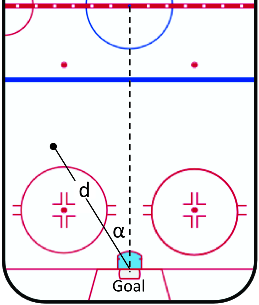
(a) Numerical specification

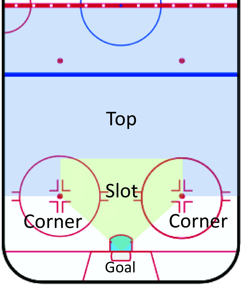
(b) Categorical specification

4 Regression models

We used multilevel logistic regression, with partial pooling, also referred to as mixed effects modelling. We center the variable of interest [6, 12] by subtracting the group mean, that is, we set $x_{ij}^{\ast}=x_{ij}-\bar{x}_{j}$, where $\bar{x}_{j}$ is the average of $x_{ij}$ in group $j$. The centered variable $x_{ij}^{\ast}$ represents the deviation in performance of the goaltender-season group $j$ from his average performance for the current playoffs. Our interest is in whether such deviations persist over time.

We allow the intercepts and the slope coefficients of the variables of interest to vary by group, but the control variable slope coefficients are the same for all groups, as shown in the following partial pooling specification:

$$\Pr(y_{ij}=1)=\mbox{logit}^{-1}(\alpha_{j}+\beta_{j}x_{ij}^{\ast}+\gamma Z_{ij}),$$ (1)

where $\mbox{logit}(p)\equiv\ln(p/(1-p))$, $\alpha_{j}$ is the intercept for group $j$, $\beta_{j}$ is the slope for group $j$, and $\gamma$ is the global vector of coefficients for the control variables. We represent the intercept and slope of the variable of interest as the sum of a fixed effect and a random effect, that is: $\alpha_{j}=\bar{\alpha}+\alpha_{j}^{\ast}$ and $\beta_{j}=\bar{\beta}+\beta_{j}^{\ast}$.

All results that we report in Section 5 were obtained using Markov chain Monte Carlo (MCMC), using the rstan and rstanarm R packages. We used the default prior distributions for the rstanarm package. The default distributions are weakly informative—Normal distributions with mean $0$ and scale $2.5$ (for the coefficients) and $10$ (for the intercepts) [7]. We used default values for the number of chains ($4$), the number of iterations (2,000), and the warm-up period (1,000 iterations).

We also used maximum likelihood (ML), using the lme4 R package, and found the MCMC and ML estimates to be nearly identical, except for a few instances where the ML estimation algorithm did not converge. The lack of ML estimation convergence in some instances is consistent with the findings in [5]. MCMC is considered a good surrogate in situations where an ML estimation algorithm has not been established [26].

5 Results

In this section, we first provide detailed results for the longest window sizes, using the categorical specification for Position. Second, we investigate the robustness of our main finding to the window size, window type, individual goaltender-seasons, and which specification was used for Position. Third, we illustrate the estimated impact of the control variables on the save probability for the next shot. Fourth, we provide diagnostics for the MCMC estimation.

5.1 Baseline results

Table 1 provides means and 95% credible intervals for the intercept and slope fixed effects and for the control variable coefficients, for our baseline models: the models with 150-shot and 300-minute windows, and a categorical specification for Position. The window sizes for the baseline models are comparable to those used by [10].

Table 1: Regression results for the 150-shot model and the 300-minute model

	$k=150$ shots			$t=300$ minutes
Variable	Mean	2.5%	97.5%	Mean	2.5%	97.5%
Intercept fixed effect	$2.10$	$1.64$	$2.57$	$2.13$	$1.67$	$2.62$
Recent save performance ($x_{ij}^{\ast}$) fixed effect	$-8.45$	$-11.64$	$-5.31$	$-8.59$	$-11.49$	$-5.53$
Game score: Tied	$-0.05$	$-0.16$	$0.06$	$-0.03$	$-0.15$	$0.08$
Game score: Trailing	$-0.12$	$-0.25$	$0.00$	$-0.11$	$-0.23$	$0.02$
Home	$-0.02$	$-0.12$	$0.09$	$0.02$	$-0.08$	$0.12$
Rebound	$-1.09$	$-1.25$	$-0.94$	$-1.10$	$-1.26$	$-0.93$
Strength: $+2$	$1.86$	$-1.22$	$5.61$	$1.82$	$-1.09$	$5.68$
Strength: $+1$	$0.76$	$0.24$	$1.28$	$0.73$	$0.22$	$1.22$
Strength: $0$	$0.94$	$0.51$	$1.36$	$0.94$	$0.52$	$1.33$
Strength: $-1$	$0.45$	$0.00$	$0.87$	$0.45$	$0.03$	$0.85$
Shot type: Deflected	$-0.98$	$-1.34$	$-0.63$	$-1.07$	$-1.41$	$-0.72$
Shot type: Slap	$-0.03$	$-0.24$	$0.18$	$-0.12$	$-0.34$	$0.09$
Shot type: Snap	$-0.05$	$-0.25$	$0.15$	$-0.11$	$-0.32$	$0.10$
Shot type: Tip-in	$-0.56$	$-0.78$	$-0.34$	$-0.62$	$-0.85$	$-0.40$
Shot type: Wrap-around	$0.40$	$-0.10$	$0.93$	$0.31$	$-0.19$	$0.83$
Shot type: Wrist	$0.02$	$-0.15$	$0.19$	$-0.04$	$-0.21$	$0.13$
Position: Top	$0.70$	$0.51$	$0.89$	$0.68$	$0.49$	$0.86$
Position: Slot	$-0.82$	$-0.94$	$-0.69$	$-0.84$	$-0.97$	$-0.71$

Our main finding from the baseline models is that a goaltender’s recent save performance has a negative and a statistically significant fixed effect value for both window sizes, which is contrary to the hot-hand theory.

The two baseline models give consistent results for the control variables. The only two control variable coefficients that disagree in sign, Home and Shot type: Wrist, have 95% credible intervals that contain zero. The posterior mean values for the significant control variables have the same sign, have similar magnitude, and are in the direction we expect, for both window types. Specifically, the posterior mean values indicate that a goaltender performs better when his team has more skaters on the ice, when facing a wrap-around shot, and when facing a shot from the top region. A goaltender performs worse when facing a rebound shot, a deflected shot, a slap shot, a snap shot, a tip-in shot, or a shot from the slot region.

5.2 Robustness of main finding

Our main finding, that recent save performance has a negative fixed effect value, holds for all window sizes and types (Figure 2). (Although not shown in the figure, all of the fixed effects are statistically significant.) The fixed effect magnitude increases with the window size.

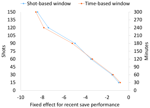
Figure 2: Recent save performance fixed effects, for all window types and sizes.

The fact that the slope fixed effects, $\hat{\bar{\beta}}$, are negative leaves open the possibility that the slopes for some individual goaltender-seasons are positive, but Figures 3-4 show that this is not the case. These figures show that all of the individual-group slope coefficients, $\hat{\beta}_{j}$, for both the longest window sizes (Figure 3) and the shortest window sizes (Figure 4), are strongly negative. Figures 3-4 also show positive correlation between the slope estimates from the shot-based vs. the time-based window models.

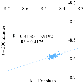
Figure 3: Estimated slopes ($\hat{\beta}_{j}$s) for all groups, for $k=150$ window vs. $t=300$ window.

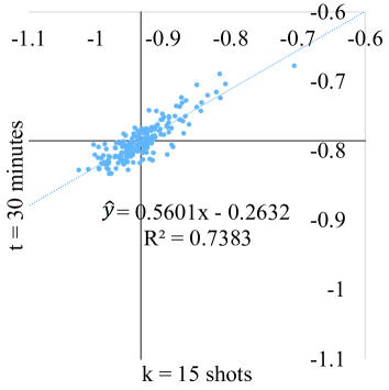
Figure 4: Estimated slopes ($\hat{\beta}_{j}$s) for all groups, for $k=15$ window vs. $t=30$ window.

The coefficients of the significant control variables remained consistent in sign and similar in magnitude across all window sizes and types (Figure 5). The control variable point estimates for all window types and sizes are within a $95\%$ Bayesian confidence interval (or a credible interval) for the 300-minute baseline model. Furthermore, changing the specification for Position from categorical to numerical, for the $t=300$ baseline model, resulted in a slope fixed effect that remained negative and was similar in magnitude. The signs of the coefficients for all statistically significant control variables in this model variant agreed with the $t=300$ baseline model.

Figure 5: Control variable slope coefficient estimates, for all window types and sizes. The point estimates are represented by small circles. $95\%$ Bayesian confidence intervals from the $t=300$-minute baseline model are included for comparison.

5.3 Magnitude of the impact of the independent variables on the save probability

Figures 6–7 illustrate the impact of recent save performance and the control variables on the estimated save probability for the next shot, using the $t$ = 300-minute baseline model. In creating Figure 6, we set all control variables to their baseline values. In creating Figure 7, for each panel, we set $x_{ij}^{\ast}=0$ and we set all control variables except the one being varied in the panel to their baseline values.

From Figure 6, we see that as the deviation of a goaltender’s recent save performance from his current-playoff average increases from the 2.5th to the 97.5th percentile, his estimated save probability for the next shot decreases by 5 pps. For comparison, this range is larger than the 3.7 pp range of average save percentages during the 2018-19 regular season (as discussed in Section 1) but smaller than the 8 pp range of average save percentages during the playoffs of the same season.

Given that we define $x_{ij}^{\ast}$ to be the deviation in performance of the goaltender-season group $j$ from his average performance for the current playoffs, the percentiles for $x_{ij}^{\ast}$ correspond to different recent save performances for different groups. To illustrate the effect in more concrete terms, consider the largest group: The 699 shots faced by Tim Thomas during the 2011 playoffs. The group average was $\bar{x}_{j}=94$%. We set each control variable category equal to its sample proportion in the group $j$ data. For shots where Thomas’ recent save performance was at the 2.5th percentile, corresponding to $x_{ij}=91.3$%, his estimated save probability for the next shot was 95.2%—a 3.9 pp increase. At the other extreme, for shots where the recent save performance was at the 97.5th percentile, corresponding to $x_{ij}=97.2$%, the estimated save probability for the next shot was 92.4%—a 4.8 pp decrease.

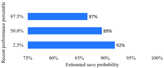
Figure 6: Estimated save probability against $2.5\rm{th}$, $50\rm{th}$ and $97.5\rm{th}$ percentile of $x_{ij}^{\ast}$, the recent save performance.

Figure 7 depicts the save probability against different values for the control variables. Home and Game score have minimal impact on the estimated save probability. Different values for Position, Rebound, Strength, and Shot type, in contrast, have a substantial impact on estimated save probability: a shot from the Slot is 16 pps less likely to be saved than a shot from the Top; a rebound shot is 15 pps less likely to be saved than a non-rebound shot; and a shot from a team that has a 2-man advantage is 9 pps less likely to be saved than shot from a team that is 2 men short. For Shot type, the save probability decreases by 18 pps when moving from wrap-around (the shot type least likely to result in a goal) to a deflected shot (the type most likely to result in a goal).

Figure 7: Control Variables versus estimated save Probability

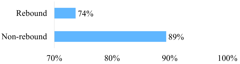
(a) Rebound

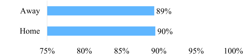
(b) Home

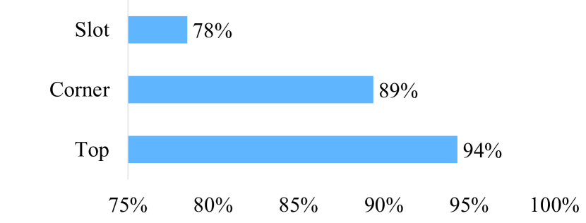
(c) Position

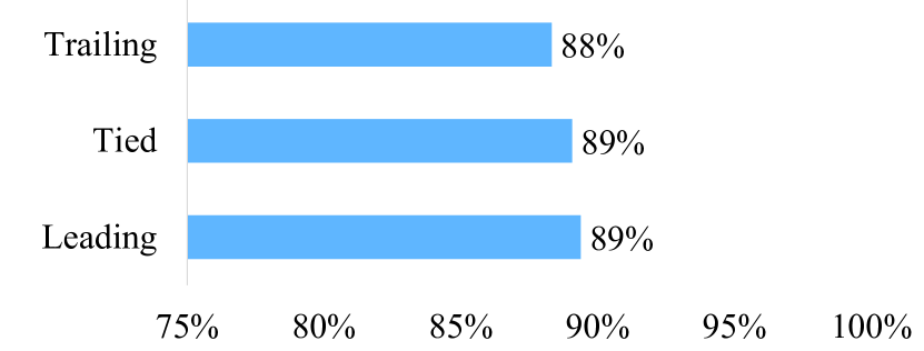
(d) Game score

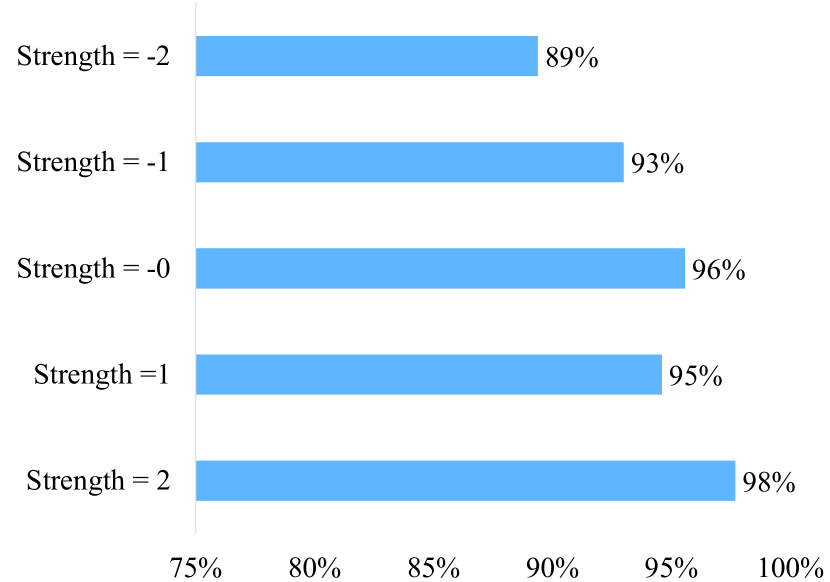
(e) Strength

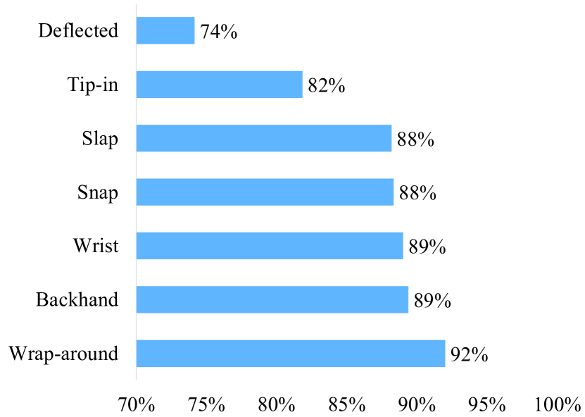
(f) Shot type

5.4 MCMC diagnostics

We computed two diagnostic statistics: $\hat{R}$ and $n_{\rm{eff}}$. To check whether a chain has converged to the equilibrium distribution we can compare the chain’s behavior to other randomly initialized chains. The potential scale reduction statistic, $\hat{R}$, allows us to perform this comparison, by computing the ratio of the average variance of draws within each chain to the variance of the pooled draws across chains; if all chains are at equilibrium, the two variances are equal and $\hat{R}=1$, and this is what we found for all of our models.

The effective sample size, $n_{\rm{eff}}$, is an estimate of the number of independent draws from the posterior distribution for the estimate of interest. The $n_{\rm{eff}}$ metric computed by the rstan package is based on the ability of the draws to estimate the true mean value of the parameter. As the draws from a Markov chain are dependent, $n_{\rm{eff}}$ is usually smaller than the total number of draws. [8] recommend running the simulation until $n_{\rm eff}$ is at least 5 times the number of chains, or $5\times 4=20$. This requirement is met for all parameters in all of our models.

6 Discussion and conclusion

We used multilevel logistic regression to investigate whether the performance of NHL goaltenders during the playoffs is consistent with a hot-hand effect. We used data from the 2008–2016 NHL playoffs. We measured past performance using both shot-based windows (as has been done in past research) and time-based windows (which has not been done before). Our window sizes spanned a wide range: from, roughly, half a game to 5 games. We allowed the intercept and the slope with respect to recent save performance to vary across goaltender-season combinations.

We found a significant negative impact of recent save performance on the next-shot save probability. This finding was consistent across all window types, window sizes, and goaltender-season combinations. This finding is inconsistent with a hot-hand effect and contrary to the findings for baseball in [10], who used a similar window size and hypothesized that skilled activity would generally demonstrate a hot-hand effect.

If a goaltender’s performance, after controlling for observable factors, was completely random, then we would expect a period of above-average or below-average recent save performance to be likely to be followed by a period of save performance that is closer to the average, because of regression to the mean. As we increase the sample size used to measure recent save performance (that is, increase the window size), we would expect the average amount by which performance moves toward the average to decrease. We observe the opposite (see Figure 2), which argues against our finding being driven by regression to the mean.

A motivation effect provides one possible explanation for our finding. That is, if a goaltender’s recent save performance has been below his average for the current playoffs, then his motivation increases, resulting in increased effort and focus, causing the next-shot save probability to be higher. Conversely, if the recent save performance has been above average, then the goaltender’s motivation, effort, and focus could decrease, leading to a lower next-shot save probability. [3] find support for the first of these effects (greater performance after failure) for “obsessively passionate individuals” but did not find support for the second effect (worse performance after success) for such individuals. The study found support for neither effect for “harmoniously passionate individuals.” These findings are consistent with Hall-of-Fame goaltender Ken Dryden’s (dryden2019life) sentiment that “if a shot beats you, make sure you stop the next one, even if it is harder to stop than the one before.” The psychological mechanisms underlying our finding could benefit from further study.

Although the estimated recent save performance coefficient is consistently negative, its magnitude varies and in particular, the magnitude increases sharply with the window size. We expect to see more reliable estimates with longer window sizes, but the increase in magnitude is surprising, given that we define the recent save performance as a scale-free save percentage.

One limitation of our study is that, in defining windows, we ignore the time that passes between games. Past research, such as [10], shares this limitation. This limitation could be particularly serious for backup goaltenders, for whom the interval between two successive appearances could be several days long.

References

- [1] S. Christian Albright “A Statistical Analysis of Hitting Streaks in Baseball” In Journal of the American Statistical Association 88.424, 1993, pp. 1175–1183
- [2] Jeremy Arkes “Revisiting the Hot Hand Theory with Free Throw Data in a Multivariate Framework” In Journal of Quantitative Analysis in Sports 6.1 De Gruyter, 2010
- [3] Jocelyn J Bélanger, Marc-André K Lafreniere, Robert J Vallerand and Arie W Kruglanski “Driven by Fear: The Effect of Success and Failure Information on Passionate Individuals’ Performance.” In Journal of Personality and Social Psychology 104.1, 2013, pp. 180–195 DOI: 10.1037/a0029585
- [4] Ken Dryden “Scotty: A Hockey Life Like No Other” McLelland & Stewart, 2019
- [5] Christopher Eager and Joseph Roy “Mixed Effects Models are Sometimes Terrible”, 2017 arXiv:1701.04858 [stat.AP]
- [6] Craig K. Enders and Davood Tofighi “Centering Predictor Variables in Cross-Sectional Multilevel Models: A New Look at an Old Issue.” In Psychological Methods 12.2, 2007, pp. 121
- [7] Jonah Gabry and Ben Goodrich “Prior Distributions for rstanarm Models”, https://cran.r-project.org/web/packages/rstanarm/vignettes/priors.html, 2019
- [8] Andrew Gelman et al. “Bayesian Data Analysis” Chapman and Hall/CRC, 2013
- [9] Thomas Gilovich, Robert Vallone and Amos Tversky “The Hot Hand in Basketball: On the Misperception of Random Sequences” In Cognitive Psychology 17.3 Elsevier, 1985, pp. 295–314
- [10] Brett Green and Jeffrey Zwiebel “The Hot-Hand Fallacy: Cognitive Mistakes or Equilibrium Adjustments? Evidence from Major League Baseball” In Management Science 64.11, 2017, pp. 5315–5348
- [11] Hockey Reference “Season Data”, http://www.hockey-reference.com/, 2017
- [12] Joop Hox and J. Kyle Roberts “Handbook of Advanced Multilevel Analysis” Psychology Press, 2011
- [13] Kevin M. Kniffin and Vince Mihalek “Within-Series Momentum in Hockey: No Returns for Running up the Score” In Economics Letters 122.3, 2014, pp. 400–402
- [14] Jeffrey A Livingston “The Hot Hand and the Cold Hand in Professional Golf” In Journal of Economic Behavior & Organization 81.1 Elsevier, 2012, pp. 172–184
- [15] Joshua B. Miller and Adam Sanjurjo “Surprised by the Hot Hand Fallacy? A Truth in the Law of Small Numbers” In Econometrica 86.6, 2018, pp. 2019–2047
- [16] Joshua B. Miller and Adam Sanjurjo “A Bridge from Monty Hall to the Hot Hand: The Principle of Restricted Choice” In Journal of Economic Perspectives 33.3, 2019, pp. 144–62
- [17] Donald G. Morrison and David C. Schmittlein “It Takes a Hot Goalie to Raise the Stanley Cup” In Chance 11.1, 1998, pp. 3–7
- [18] Marius Ötting and Andreas Groll “A Regularized Hidden Markov Model for Analyzing the ‘Hot Shoe’ in Football” In arXiv preprint arXiv:1911.08138, 2019
- [19] Marius Ötting, Roland Langrock, Christian Deutscher and Vianey Leos-Barajas “The Hot Hand in Professional Darts” In Journal of the Royal Statistical Society: Series A (Statistics in Society) 183.2, 2020, pp. 565–580
- [20] Emmanuel Perry “Corsica Play-by-Play Data”, http://www.corsica.hockey/data/, 2017
- [21] Amos Tversky and Thomas Gilovich “The Cold Facts about the ‘Hot Hand’ in Basketball” In Chance 2.1, 1989, pp. 16–21
- [22] Amos Tversky and Thomas Gilovich “The ‘Hot Hand’: Statistical Reality or Cognitive Illusion?” In Chance 2.4, 1989, pp. 31–34
- [23] Andrew Vesper “Putting the ‘Hot Hand’ on Ice” In Chance 28.2, 2015, pp. 13–18
- [24] Robert L Wardrop “Simpson’s Paradox and the Hot Hand in Basketball” In The American Statistician 49.1, 1995, pp. 24–28 DOI: 10.1080/00031305.1995.10476107
- [25] Robert L Wardrop “Statistical Tests for the Hot-Hand in Basketball in a Controlled Setting” In Unpublished manuscript 1, 1999, pp. 1–20
- [26] James A. Wollack, Daniel M. Bolt, Allan S. Cohen and Young-Sun Lee “Recovery of Item Parameters in the Nominal Response Model: A Comparison of Marginal Maximum Likelihood Estimation and Markov Chain Monte Carlo Estimation” In Applied Psychological Measurement 26.3, 2002, pp. 339–352