Community Structure Recovery
and Interaction Probability Estimation
for Gossip Opinion Dynamics

Abstract

We study how to jointly recover the community structure and estimate the interaction probabilities of gossip opinion dynamics. In this process, agents randomly interact pairwise, and there are stubborn agents never changing their states. Such a model illustrates how disagreement and opinion fluctuation arise in a social network. It is assumed that each agent is assigned with one of two community labels, and the agents interact with probabilities depending on their labels. The considered problem is to jointly recover the community labels of the agents and estimate interaction probabilities between the agents, based on a single trajectory of the model. We first study stability and limit theorems of the model, and then propose a joint recovery and estimation algorithm based on a trajectory. It is verified that the community recovery can be achieved in finite time, and the interaction estimator converges almost surely. We derive a sample-complexity result for the recovery, and analyze the estimator’s convergence rate. Simulations are presented for illustration of the performance of the proposed algorithm.

, , [cor1]Corresponding author. ,

1 Introduction

Networks appear across domains from biology to sociology. Real networks often exhibit community structures, where subsets of nodes have dense connections locally but sparse connections globally [1]. Community detection is to partition nodes according to the network topology. There is a growing interest in studying community detection based on state observations of dynamics [2, 3, 4, 5, 6, 7]. Lacking topology data makes the problem harder than classic ones. Particularly, it is unclear how to recover communities out of a single trajectory of opinion dynamics [8].

1.1 Related work

In this subsection, we first review key community definitions and detection approaches [1], then discuss recovering communities based on state observations, and finally clarify our motivation.

Traditional community detection methods apply classic clustering techniques to node pairs assigned with certain weights [9]. In [10], the authors introduce the concept of modularity to measure the quality of a graph partition. A famous algorithm based on optimizing modularity is the Louvain method [11], which assigns nodes to one of the communities iteratively to achieve the largest modularity gain. Another approach to community detection is based on statistical inference, which introduces generative network models and considers an observed network as a sample. A canonical model is the stochastic block model (SBM). The paper [12] reviews results on detectability of the SBM and performance of algorithms. Besides optimization and statistical approaches, another method is based on dynamical processes (e.g., [13]). The paper [14] proposes a bounded-confidence model, where agents converge to several clusters corresponding to communities.

Recently, the study of community detection for networked dynamics has emerged. The problem is to recover communities only based on state observations of a dynamical process. The main difference between this problem and the classic ones, especially the dynamic-based methods, is that the network is not available. The papers [2, 7] apply maximum likelihood methods to cascade data. The paper [2] also proposes a two-step procedure, first constructing a network and then clustering agents based on the network. The authors of [4, 5, 6] introduce the blind community detection method, using sample covariance matrices of agent states for recovery. The author in [3] investigates simultaneously reconstructing the topology and the community structure for epidemics and the Ising model. The paper [15] studies recovery for an Ising blockmodel.

We study how to jointly recover the community structure and estimate the interaction probabilities of gossip opinion dynamics. The problem arises from recent investigation of learning interpersonal influence from dynamics [8]. Network data is useful for decision making, but directly collecting such data can be hard, due to topic specificity [16], consistency issues [17], and privacy concern [18]. Learning large-scale networks may be computationally expensive, so recovering communities as a coarse description is a good option. The gossip update rule captures the random nature of individual interactions. It is a fundamental element of many opinion models [19], and has also been extensively studied [20]. Stubborn agents, such as media and opinion leaders, play a crucial role in opinion formation [21]. The paper [22] shows that the existence of stubborn agents can explain opinion oscillation. A generalization of stubborn agents is to assume that each agent has some level of stubbornness with respect to its initial belief. This generalization is considered by the Friedkin–Johnsen model and its extensions [23, 24].

1.2 Contributions

We consider jointly recovering communities and estimating interaction probabilities for gossip opinion dynamics. Each agent is assigned with one of the two community labels, and the agents interact with probabilities depending on their labels. Our contributions are as follows:

1. We study properties of the model by leveraging results on Markov chains and stochastic approximation (SA) (Theorem 8). It is shown that regular-agent states converge in distribution to a unique stationary distribution, and the time average of the agent states converge almost surely. An explicit expression for the mean of the stationary distribution is given (Proposition 10).
2. We develop a joint algorithm (Algorithm 1) to recover the community structure and to estimate the interaction probabilities, based on Polyak averaging and SA techniques. The algorithm is able to recover the communities in finite time, and then able to estimate the interaction probabilities consistently (Theorem 16).
3. We show how to theoretically analyze the developed joint algorithm. A concentration inequality for Markov chains (Lemma 18) is obtained, and it is used in the sample-complexity analysis of the recovery step (Theorem 20). The obtained result shows that the probability of unsuccessful recovery decays exponentially over time. Additionally, we analyze convergence rate of the interaction estimator from an SA argument (Theorem 22).

The obtained results indicate that a Polyak averaging technique can be useful for recovering communities based on a single trajectory. In addition, we establish a sample-complexity result for successful recovery (recovering all community labels correctly), providing a quantitative dependence of the successful recovery probability on model parameters. These two points make our paper different from [4, 5, 6], which use covariance matrices of samples from several trajectories, and different from [25], which considers learning a sparse characterization of the network from the gossip model. The considered problem is different from classic system identification (e.g., [26]), because stubborn agents normally have fixed states, which does not satisfy input conditions required for system identification, and also because community recovery cannot be obtained directly from parameter estimates. The major differences between this paper and its conference version [27] are that we clarify our assumptions in more detail, characterize the sample complexity and the convergence rate of the algorithm, and add more numerical experiments to illustrate its performance.

1.3 Outline

The rest of the paper is organized as follows. Section 2 formulates the problem. Analysis of the model is given in Section 3, and a joint recovery and estimation algorithm is proposed in Section 4. Section 5 presents convergence results of the algorithm, and Section 6 provides several numerical experiments. Finally, Section 7 concludes the paper. Some proofs are postponed to appendices.

Notation. Denote the $n$-dimensional Euclidean space by $\mathbb{R}^{n}$, the set of $n\times m$ real matrices by $\mathbb{R}^{n\times m}$, the set of nonnegative integers by $\mathbb{N}$, and the set of positive integers by $\mathbb{N}^{+}$. Let $\mathbf{1}_{n}$ be the all-one vector with dimension $n$, $\textbf{e}_{i}$ be the unit vector with $i$-th entry being one, $I_{n}$ be the $n\times n$ identity matrix, and $\mathbf{0}_{n,m}$ be the $n\times m$ all-zero matrix. Define $\mathbf{1}_{n_{1},n_{2}}:=\mathbf{1}_{n_{1}}\mathbf{1}_{n_{2}}^{T}$, where $A^{T}$ represents the transpose of a matrix $A$. Denote the Euclidean norm of a vector by $\|\cdot\|$, and denote the maximum absolute column sum norm, spectral norm, and maximum absolute row sum norm of a square matrix by $\|\cdot\|_{1}$, $\|\cdot\|$, and $\|\cdot\|_{\infty}$. Denote the diagonal matrix with the elements of a vector $x$ on the main diagonal by $\text{diag}\{x\}$.

For a vector $x\in\mathbb{R}^{n}$, denote its $i$-th component by $x_{i}$, and for a matrix $A=[a_{ij}]_{1\leq i,j\leq n}\in\mathbb{R}^{n\times n}$, denote its $(i,j)$-th entry by $a_{ij}$ or $[A]_{ij}$. The matrix $A$ is said to be row stochastic if $a_{ij}\geq 0$ and $A\mathbf{1}=\mathbf{1}$, and to be substochastic if $a_{ij}\geq 0$ and the row sums of $A$ are not larger than one. Denote the spectral radius of $A$ by $\rho(A)$. The cardinality of a set $\Omega$ is denoted by $|\Omega|$. The function $\mathbb{I}_{[\textup{property}]}$ is the indicator function equal to one if the property in the bracket holds, and equal to zero otherwise. For two sequences $\{a_{k}\}$ and $\{b_{k}\}$ with $a_{k}\in\mathbb{R}^{n}$ and $0\not=b_{k}\in\mathbb{R}$, $k\geq 1$, $a_{k}=O(b_{k})$ means that $\|a_{k}/b_{k}\|\leq C$ for all $k$ and some $C>0$, and $a_{k}=o(b_{k})$ means that $\lim_{k\to\infty}\|a_{k}/b_{k}\|=0$. An event happens almost surely (a.s.) if it happens with probability one. $\mathbb{E}\{X\}$ is the expectation of the random vector $X$. The notation $\overset{\textup{d}}{\to}$ represents convergence in distribution.

To define a Markov chain taking values on $(\mathbb{R}^{n},\mathcal{B}(\mathbb{R}^{n}))$, where $\mathcal{B}(\mathbb{R}^{n})$ is the Borel $\sigma$-field, we first define the transition probability kernel $P(x,A)$, $x\in\mathbb{R}^{n}$, $A\in\mathcal{B}(\mathbb{R}^{n})$, satisfying that for each $A\in\mathcal{B}(\mathbb{R}^{n})$, $P(\cdot,A)$ is a non-negative measurable function on $\mathbb{R}^{n}$, and for each $x\in\mathbb{R}^{n}$, $P(x,\cdot)$ is a probability measure on $\mathcal{B}(\mathbb{R}^{n})$. A (homogeneous) Markov chain $\{X(t),t\in\mathbb{N}\}$ on $\mathbb{R}^{n}$ satisfies that for all $t\in\mathbb{N}$, $A\in\mathcal{B}(\mathbb{R}^{n})$, and $x\in\mathbb{R}^{n}$,

$$\mathbb{P}\{X(t+1)\in A|X(t)=x,X(t-1)\dots,X(0)\}$$

$$=\mathbb{P}\{X(t+1)\in A|X(t)=x\}=P(x,A).$$

Using transition probability kernel $P(\cdot,\cdot)$, we can define $n$-step transition probability of $\{X(t)\}$ inductively by

$$P^{t}(x,A)=\int_{\mathbb{R}^{n}}P(x,dy)P^{t-1}(y,A),~{}t\in\mathbb{N}^{+},$$

and $P^{0}(x,A)=\mathbb{I}_{[x\in A]}$, for all $x\in\mathbb{R}^{n}$ and $A\in\mathcal{B}(\mathbb{R}^{n})$. A stationary distribution of a Markov chain $\{X(t)\}$ with transition probability kernel $P(\cdot,\cdot)$ is a probability measure $\pi$ on $\mathcal{B}(\mathbb{R}^{n})$ such that

$$\pi(A)=\int_{\mathbb{R}^{n}}\pi(dx)P(x,A),\quad A\in\mathcal{B}(\mathbb{R}^{n}).$$

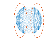
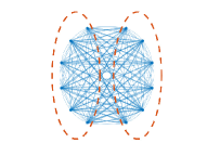
(a) The left (right) graph demonstrates the case where $w_{s}>w_{d}$ ($w_{s}<w_{d}$), in which agents within the same community interacting more (less) often than agents between communities. The width of edges is proportional to the number of interactions.

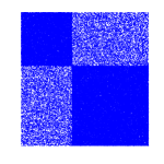
(b) The adjacency matrix of a graph generated from $\textup{SBM}(n,\nu_{1},\nu_{2},p_{s},p_{d})$ with $n=5000$, $\nu_{1}=0.4$, $\nu_{2}=0.6$, $p_{s}=5\log n/n$, $p_{d}=\log n/n$. Dots represent nonzero entries, so the block structure of the matrix is clearly visible.

Figure 1: Illustration of the interaction model (4) and an adjacency matrix generated from an SBM.

2 Problem Formulation

This section introduces the considered model and the definition of communities, and formulates the problem.

2.1 Gossip Model with Stubborn Agents

The gossip model is a random process over an undirected graph $\mathcal{G}=(\mathcal{V},\mathcal{E})$ with the agent set $\mathcal{V}$, the edge set $\mathcal{E}$, and no self-loops. The agents have two types, regular and stubborn, denoted by $\mathcal{V}_{r}$ and $\mathcal{V}_{s}$, respectively ($\mathcal{V}=\mathcal{V}_{r}\cup\mathcal{V}_{s}$, $\mathcal{V}_{r}\cap\mathcal{V}_{s}=\emptyset$). Each agent $i$ has a state $X_{i}(t)\in\mathbb{R}$, and the state vector at time $t\in\mathbb{N}$ is $X(t)\in\mathbb{R}^{n}$. Stubborn agents do not change their states during the process.

An interaction probability matrix $W=[w_{ij}]\in\mathbb{R}^{n\times n}$ captures agent interactions, where $w_{ij}=w_{ji}\geq 0$, $w_{ij}>0\Leftrightarrow\{i,j\}\in\mathcal{E}$, $i,j\in\mathcal{V}$, and $\mathbf{1}^{T}W\mathbf{1}/2=$ $1$. At time $t$, edge $\{i,j\}$ is selected with probability $w_{ij}$ independently of previous updates, and agents update as follows, with the averaging weight $q\in[0,1)$,

$$X_{k}(t+1)=\begin{cases}qX_{k}(t)+(1-q)X_{l}(t),&\text{if }k\in\mathcal{V}_{r}\cap\{i,j\},\\ &l\in\{i,j\}\setminus k,\\ X_{k}(t),&\text{otherwise}.\end{cases}$$ (1)

For $1\leq i<j\leq n$, define

$$R^{ij}=$$

$$\begin{cases}I-(1-q)(\textbf{e}_{i}-\textbf{e}_{j})(\textbf{e}_{i}-\textbf{e}_{j})^{T},&\text{if }i,j\in\mathcal{V}_{r},\\ I-(1-q)\textbf{e}_{i}(\textbf{e}_{i}-\textbf{e}_{j})^{T},&\text{if }i\in\mathcal{V}_{r},j\in\mathcal{V}_{s},\\ I-(1-q)\textbf{e}_{j}(\textbf{e}_{j}-\textbf{e}_{i})^{T},&\text{if }i\in\mathcal{V}_{s},j\in\mathcal{V}_{r},\\ I,&\text{if }i,j\in\mathcal{V}_{s},\end{cases}$$

and a sequence of independent and identically distributed (i.i.d.) $n$-dimensional random matrices $\{R(t),$ $t\in\mathbb{N}\}$ such that $\mathbb{P}\{R(t)=R^{ij}\}=w_{ij}$, $1\leq i<j\leq n.$ The update rule (1) can then be written as

$$X(t+1)=R(t)X(t).$$ (2)

Since stubborn agents never change their states, we rewrite (2) to end up with the following compact form of the gossip model with stubborn agents:

$$X^{r}(t+1)=A(t)X^{r}(t)+B(t)X^{s}(t),$$ (3)

where $X^{r}(t)$ and $X^{s}(t)$ are the state vectors obtained from stacking the states of regular and stubborn agents, respectively, $X^{s}(t)\equiv X^{s}(0)$, and $[A(t)~{}B(t)]$ is the matrix obtained from stacking rows of $R(t)$ corresponding to regular agents. So $\{[A(t)~{}B(t)],t\in\mathbb{N}\}$ is a sequence of i.i.d. random matrices. Assume that the initial vector $X(0)$ is fixed, for simplicity. If $X(0)$ is random, we can study the model by conditioning on realizations of $X(0)$.

2.2 Communities

We follow the framework of SBMs [12] and Ising blockmodels [15], and assume that agents have pre-assigned community labels. We define a community as the set of agents that have the same label.

In particular, we consider the scenario where the network has two disjoint communities, $\mathcal{V}_{1}$ and $\mathcal{V}_{2}$. Denote the community label of $i$ by $\mathcal{C}(i)$, so $\mathcal{C}(i)=k$ for $i\in\mathcal{V}_{k}$, $k=1,2$. We call $\mathcal{C}$ the community structure of the network. We further assume that the interaction probability of the agents $i$ and $j$ with $i\not=j$ is

$$w_{ij}=\begin{cases}w_{s},&\text{ if }\mathcal{C}(i)=\mathcal{C}(j),\\ w_{d},&\text{ if }\mathcal{C}(i)\not=\mathcal{C}(j),\end{cases}$$ (4)

where $w_{s},w_{d}\in(0,1)$ and $w_{s}\not=w_{d}$. Thus agents in the same community (different communities) interact with probability $w_{s}$ ($w_{d}$). Fig. 1(a) illustrates two different interaction models, via a simulation where a gossip model defined by (4) is run for $2000$ iterations and the number of interactions between agents is counted. To ease notation, we assume that $\mathcal{V}_{1}=\{1,\dots,n_{1}\}$ and $\mathcal{V}_{2}=\{n_{1}+1,\dots,n_{1}+n_{2}\}$ with $n_{k}:=|\mathcal{V}_{k}|$, $k=1,2$, and $n_{1}+n_{2}=n$. Thus the interaction probability matrix is

$$W=\begin{bmatrix}w_{s}\mathbf{1}_{n_{1},n_{1}}-\text{diag}\{w_{s}\mathbf{1}_{n_{1}}\}&w_{d}\mathbf{1}_{n_{1},n_{2}}\\ w_{d}\mathbf{1}_{n_{2},n_{1}}&w_{s}\mathbf{1}_{n_{2},n_{2}}-\text{diag}\{w_{s}\mathbf{1}_{n_{2}}\}\end{bmatrix}$$ (5)

It has a block structure corresponding to the community structure of the network.

The following example illustrates how the preceding assumption arises naturally from an SBM. It shows that a graph generated from an SBM defines an interaction probability matrix close to an averaged version with the same structure as (5).

Example 1.

Consider an SBM with two communities, commonly studied in community detection [12]. Such an SBM is a random graph, denoted by $\textup{SBM}(n,\nu_{1},\nu_{2},p_{s},p_{d})$. Here $n$ is the number of agents, $\nu_{1}\in(0,1)$ (resp. $\nu_{2}\in(0,1)$) is the portion of agents with community label $1$ (resp. label $2$), where $\nu_{1}+\nu_{2}=1$ and $\nu_{1}n$ and $\nu_{2}n$ are integers, and $p_{s},p_{d}\in(0,1)$ are the link probabilities between agents in the same and in different communities. We assume $\mathcal{C}(i)=1$, $1\leq i\leq\nu_{1}n$, and $\mathcal{C}(i)=2$, $\nu_{1}n+1\leq i\leq n$.

The $\textup{SBM}(n,\nu_{1},\nu_{2},p_{s},p_{d})$ randomly generates an undirected graph $\mathcal{G}=(\mathcal{V},\mathcal{E},\mathcal{A})$: for $i\not=j$, $\{i,j\}\in\mathcal{E}$ with probability $p_{s}$ if $\mathcal{C}(i)=\mathcal{C}(j)$ and with probability $p_{d}$ if $\mathcal{C}(i)\not=\mathcal{C}(j)$, independently of other edges. Here $A=[a_{ij}]$ is the adjacency matrix. The graph $\mathcal{G}$ defines a gossip model with the interaction matrix $\tilde{W}=\mathcal{A}/\alpha$ and $\alpha=\sum_{i=1}^{n}\sum_{j=i+1}^{n}a_{ij}=|\mathcal{E}|$. The inequality

$$\bigg{\|}\tilde{W}-\frac{\mathbb{E}\{\mathcal{A}\}}{\mathbb{E}\{\alpha\}}\bigg{\|}\leq\frac{C}{n}$$

holds with a constant $C$, except for a probability vanishing as $n\to\infty$, if $\log n/n=O(\min\{p_{s},p_{d}\})$ (see Appendix A for a proof). This result implies that, if the network of the gossip model is generated from the SBM, then the interaction probability matrix of the gossip model is close to $\mathbb{E}\{\mathcal{A}\}/\mathbb{E}\{\alpha\}$ when $n$ is large. Note that $\mathbb{E}\{\mathcal{A}\}/\mathbb{E}\{\alpha\}$ has exactly the same structure as $W$ in (5) with $n_{k}=\nu_{k}n$, $k=1,2$, $w_{s}=p_{s}/\mathbb{E}\{\alpha\}$, and $w_{d}=p_{d}/\mathbb{E}\{\alpha\}$. Fig. 1(b) demonstrates this concentration phenomenon with an obvious two-block structure. The concentration indicates that behavior of the gossip model over a graph generated from the SBM may not deviate too far from the gossip model over the averaged graph, when $n$ is large. In fact, in [28] we show that the expected stationary states of the two models are close, if $\log n/n=o(\min\{p_{s},p_{d}\})$. This result indicates that the gossip model over the averaged graph can be considered as an approximation of the model over the SBM, and results for the former model can be extended to the latter model.

Remark 2.

A general assumption for community labels in the SBM is that each agent gets a label $k$ with probability $\nu_{k}$ independently of each other, $k=1,2$. This is essentially equivalent to the label assignment with deterministic node portions when $n\to\infty$ (Remark 3 of [12]). Note that it is possible to extend the fixed-label assumption considered in Example 1 to the deterministic-portion assumption, by conditioning on each assignment and using the law of total probability. The condition $\log n/n=O(\min\{p_{s},p_{d}\})$ implies that the expected agent degree is at least $O(\log n)$. In this case, the SBM generates connected graphs with high probability. The difference between $p_{s}$ and $p_{d}$ has to be large enough to make exact recovery possible [12]. Here we consider the dynamics over the averaged graph, so the detectability only requires $w_{s}\not=w_{d}$ (Assumption 4 (ii)). Future work will study detectability in the SBM case.

2.3 Community Recovery and Interaction Estimation

The considered problem is to recover the community structure and to estimate the interaction probabilities based on state observations, as follows.

Problem. Given a trajectory of the gossip model with the interaction matrix (5), develop an algorithm to jointly recover the community structure $\mathcal{C}$ and estimate the interaction probabilities $w_{s}$ and $w_{d}$.

Remark 3.

In the preceding problem, we assume that the developed algorithm uses data coming from the gossip model over the averaged graph. A natural question is how this algorithm performs if it uses a trajectory of the gossip model over a graph sampled from an SBM. In Section 6, we illustrate through simulation that the algorithm performs well also in the SBM case. Such performance is guaranteed by that these two processes behave similarly in terms of their stationary states, as explained in Example 1. We use “community recovery” instead of “community detection” to avoid ambiguity, following the terminology of [15], because here agent behavior depends directly on the community structure.

Recall $\mathcal{V}_{1}=\{1,\dots,n_{1}\}$ and $\mathcal{V}_{2}=\{n_{1}+1,\dots,n_{1}+n_{2}\}$. We further sort the agents as follows: $\mathcal{V}_{r1}=\{1,\dots,n_{r1}\}$, $\mathcal{V}_{s1}=\{n_{r1}+1,\dots,n_{1}\}$, $\mathcal{V}_{r2}=\{n_{1}+1,\dots,n_{1}+n_{r2}\}$, and $\mathcal{V}_{s2}=\{n_{1}+n_{r2}+1,\dots,n\}$. Here, $\mathcal{V}_{rk}$ (resp. $\mathcal{V}_{sk}$) is the set of regular (resp. stubborn) agents in the community $k$, $k=1,2$. Denote $n_{rk}:=|\mathcal{V}_{rk}|$, $n_{sk}:=|\mathcal{V}_{sk}|$, $n_{r}:=|\mathcal{V}_{r}|$, and $n_{s}:=|\mathcal{V}_{s}|$. In the considered problem, the total number of agents is known in advance, the network has two communities, and the stubborn-agent states are observable. But difficulty still remains since $n_{k}$, $n_{rk}$, $n_{sk}$, $k=1,2$, and interaction information are unknown. The interaction information cannot be obtained in general situations (e.g., agent states are only observed at some time steps, or observations are corrupted by noise, as discussed in Remark 17).

3 Model analysis

This section studies model behavior, and provides an explicit expression for the mean of the stationary distribution. Assumptions are summarized as follows.

Assumption 4.

(i.1) The agent set $\mathcal{V}$ consists of two communities, $\mathcal{V}_{1}=\{1,\dots,n_{1}\}$ and $\mathcal{V}_{2}=\{n_{1}+1,\dots,n_{1}+n_{2}\}$ with $n_{1},n_{2}>0$ and $n_{1}+n_{2}=n$.
(i.2) Both communities have regular agents, namely, $1\leq n_{r1}\leq n_{1}$, $1\leq n_{r2}\leq n_{2}$.
(ii) The interaction probability matrix $W$ has a block structure (5) with $w_{s},w_{d}>0$, $w_{s}\not=w_{d}$, and

$$(n_{1}(n_{1}-1)+n_{2}(n_{2}-1))w_{s}+2n_{1}n_{2}w_{d}=2.$$ (6)

(iii) $X(0)$ is deterministic. It holds that $X^{r}(0)\in\mathcal{S}$ with

$$\mathcal{S}:=\{x^{r}\in\mathbb{R}^{n_{r}}:x_{i}^{r}\in[\underline{s},\overline{s}],1\leq i\leq n_{r}\},$$ (7)

where $\underline{s}:=\min_{1\leq i\leq n_{s}}\{\mathbf{x}_{i}^{s}\}$, $\overline{s}:=\max_{1\leq i\leq n_{s}}\{\mathbf{x}_{i}^{s}\}$, $\mathbf{x}^{s}:=X^{s}(0)=[(\mathbf{x}^{s1})^{T}~{}(\mathbf{x}^{s2})^{T}]^{T}$ is the stubborn state vector, and $\mathbf{x}^{sk}$ is the vector for the community $k$, $k=1,2$.

$$\bar{A} =I_{n_{r}}-(1-q)\begin{bmatrix}a_{1}I_{n_{r1}}-w_{s}\mathbf{1}_{n_{r1},n_{r1}}&-w_{d}\mathbf{1}_{n_{r1},n_{r2}}\\ -w_{d}\mathbf{1}_{n_{r2},n_{r1}}&a_{2}I_{n_{r2}}-w_{s}\mathbf{1}_{n_{r2},n_{r2}}\end{bmatrix},\quad\bar{B}=(1-q)\begin{bmatrix}w_{s}\mathbf{1}_{n_{r1},n_{s1}}&w_{d}\mathbf{1}_{n_{r1},n_{s2}}\\ w_{d}\mathbf{1}_{n_{r2},n_{s1}}&w_{s}\mathbf{1}_{n_{r2},n_{s2}}\end{bmatrix},$$ (8)

$$a_{k} =w_{s}n_{k}+w_{d}n_{3-k},~{}k=1,2.$$

Remark 5.

In Assumption 4 (i.1), the order of agents is sorted for convenience, but we do not know which group each agent belongs to, before community recovery. It is necessary to assume $w_{s}\not=w_{d}$. Otherwise, $W$ has no block structure. Regular agents are assumed to start from $\mathcal{S}$, which is reasonable and intuitively means that regular states lie between the extreme stubborn states.

Before studying model behavior, we explicitly write the block structures of $\bar{A}:=\mathbb{E}\{A(t)\}$ and $\bar{B}:=\mathbb{E}\{B(t)\}$ in the following proposition, which says that the block structure of $W$ results in similar agent updates in the same community.

Proposition 6.

Suppose Assumption 4 holds. Then $\bar{A}$ and $\bar{B}$ have block structures given in (8).

For $i<j$, $i,j\in\mathcal{V}_{r}$, $R(t)=R^{ij}=I-(1-q)(\textbf{e}_{i}-\textbf{e}_{j})(\textbf{e}_{i}-\textbf{e}_{j})^{T}$ with probability $w_{ij}$, so $\bar{r}_{ij}=(1-q)w_{ij}$, where $\bar{r}_{ij}$ (resp. $w_{ij}$) is the $(i,j)$-th entry of $\bar{R}$ (resp. $W$). If $i$ and $j$ are in the same community, then $w_{ij}=w_{s}$. Otherwise, $w_{ij}=w_{d}$. The values of other off-diagonal entries of $\bar{R}$ can be obtained by following the same argument and the definition of $R^{ij}$. For the diagonal entries of $\bar{R}$, note that $R(t)$ is row stochastic a.s., so $\bar{r}_{ii}=1-\sum_{j\not=i}\bar{r}_{ij}$. By comparing $R(t)$ with $A(t)$ and $B(t)$ in the gossip model, we can obtain (8). $\Box$

Corollary 7.

If Assumption 4 holds and there exists at least one stubborn agent in the network (i.e., $n_{r}<n$), then $\bar{A}$ is Schur stable, namely, $\rho(\bar{A})<1$.

We know from Proposition 6 that $\bar{A}$ has the form (8). If there exists at least one row of $\bar{A}$ with row sum less than one. So from Lemma 31 in Appendix D, the corollary follows. $\Box$

Now we provide the stability and limit theorems of the gossip model.

Theorem 8.

(Stability and limit theorems) Suppose that Assumption 4 holds and there exists at least one stubborn agent in the network (i.e., $n_{r}<n$). The following results hold for the gossip model with stubborn agents.
(i) The model has a unique stationary distribution $\pi$ with mean $\mathbf{x}^{r}$, and $X^{r}(t)\overset{\textup{d}}{\to}\pi$, as $t\to\infty$.

(ii) The expectation of the state vector converges to $\mathbf{x}^{r}$:

$$\mathbf{x}^{r}=\lim_{t\to\infty}\mathbb{E}\{X^{r}(t)\}=(I-\bar{A})^{-1}\bar{B}\mathbf{x}^{s}.$$ (9)

(iii) Denote $S^{r}(t):=\frac{1}{t}\sum_{i=0}^{t-1}X^{r}(i)$, then

$$\lim_{t\to\infty}S^{r}(t) =\mathbf{x}^{r}\quad\text{a.s.,}$$ (10)

See Appendix D. $\Box$

Remark 9.

The first two results show that the agent states, although may not converge a.s., converge in distribution to a unique stationary distribution, and their expectations converge to the mean of the stationary distribution. The third result indicates that we can obtain the value of $\mathbf{x}^{r}$ by computing the state time average.

The next proposition shows that $\mathbf{x}^{r}$ also has a block structure, indicating that regular agents in the same community behave similarly on average.

Proposition 10.

Under the conditions of Theorem 8,

$$(I-\bar{A})^{-1}=(1-q)^{-1}$$

$$\begin{bmatrix}\frac{1}{a_{1}}(I_{n_{r1}}+\tilde{w}_{s1}\mathbf{1}_{n_{r1},n_{r1}})&\tilde{w}_{d}\mathbf{1}_{n_{r1},n_{r2}}\\ \tilde{w}_{d}\mathbf{1}_{n_{r2},n_{r1}}&\frac{1}{a_{2}}(I_{n_{r2}}+\tilde{w}_{s2}\mathbf{1}_{n_{r2},n_{r2}})\end{bmatrix},$$

where for $k=1,2$, $a_{k}=w_{s}n_{k}+w_{d}n_{3-k}$, $\tilde{w}_{d}=w_{d}/\delta$,

$$\tilde{w}_{sk} =(w_{s}^{2}n_{s,3-k}+w_{s}w_{d}n_{k}+w_{d}^{2}n_{r,3-k})/\delta,$$

$$\delta =w_{s}^{2}n_{s1}n_{s2}+w_{s}w_{d}(n_{1}n_{s1}+n_{2}n_{s2})$$

$$\quad+w_{d}^{2}(n_{1}n_{2}-n_{r1}n_{r2}).$$ (11)

As a result,

$$\mathbf{x}^{r} =\frac{1}{\delta}[(\gamma_{11}\mathbf{1}_{n_{s1}}^{T}\mathbf{x}^{s1}+\gamma_{12}\mathbf{1}_{n_{s2}}^{T}\mathbf{x}^{s2})\mathbf{1}_{n_{r1}}^{T},$$

$$\quad(\gamma_{21}\mathbf{1}_{n_{s1}}^{T}\mathbf{x}^{s1}+\gamma_{22}\mathbf{1}_{n_{s2}}^{T}\mathbf{x}^{s2})\mathbf{1}_{n_{r2}}^{T}]^{T}$$

$$:=[\chi_{1}\mathbf{1}_{n_{r1}}^{T},~{}\chi_{2}\mathbf{1}_{n_{r2}}^{T}]^{T},$$ (12)

where $\mathbf{x}^{r}$ is given in (9),

$$\gamma_{kk} =w_{s}^{2}n_{s,3-k}+w_{s}w_{d}n_{k}+w_{d}^{2}n_{r,3-k},$$

$$\gamma_{k,3-k} =w_{d}(w_{s}n_{3-k}+w_{d}n_{k}),$$

and $\mathbf{1}_{n_{sk}}^{T}\mathbf{x}^{sk}$ is defined to be zero if $n_{sk}=0$, $k=1,2$.

From (8), we have that

$$I-\bar{A}=$$

$$(1-q)\begin{bmatrix}a_{1}I_{n_{r1}}-w_{s}\mathbf{1}_{n_{r1},n_{r1}}&-w_{d}\mathbf{1}_{n_{r1},n_{r2}}\\ -w_{d}\mathbf{1}_{n_{r2},n_{r1}}&a_{2}I_{n_{r2}}-w_{s}\mathbf{1}_{n_{r2},n_{r2}}\end{bmatrix}.$$

By Corollary 7, $(I-\bar{A})^{-1}$ exists, and direct computation implies the first conclusion. Hence,

$$(I-\bar{A})^{-1}\bar{B}=\begin{bmatrix}\tilde{w}_{s1}\mathbf{1}_{n_{r1},n_{s1}}&a_{2}\tilde{w}_{d}\mathbf{1}_{n_{r1},n_{s2}}\\ a_{1}\tilde{w}_{d}\mathbf{1}_{n_{r2},n_{s1}}&\tilde{w}_{s2}\mathbf{1}_{n_{r2},n_{s2}}\end{bmatrix}.$$

Then under Assumption 4, (12) is obtained from (9). $\Box$

Remark 11.

In Appendix B, we study the block structure of $\mathbf{x}^{r}$ in a multiple-community case, as a generalization of Proposition 10.

The above proposition means that regular agents in the same community have the same limit, which is a weighted average of stubborn states. Hence it is possible to split regular agents by computing the state time average. However, we are unable to do so if only one community has stubborn agents, or the stubborn states are similar. The following condition rules out these cases.

Assumption 12.

Both communities have stubborn agents (i.e., $n_{s1}n_{s2}>0$), and $\mathbf{x}^{s}=[(\mathbf{x}^{s1})^{T}~{}(\mathbf{x}^{s2})^{T}]^{T}$ satisfies that $\mathbf{1}_{n_{s1}}^{T}\mathbf{x}^{s1}/n_{s1}\not=\mathbf{1}_{n_{s2}}^{T}\mathbf{x}^{s2}/n_{s2}$.

This assumption has a practical meaning: stubborn agents are distributed among communities, and agents from different communities are more likely to have distinct opinions. Under Assumption 12, we have the following result, indicating that the presence of stubborn agents enhances the separation of regular agents.

Proposition 13.

Under the conditions of Theorem 8, $\chi_{1}\not=\chi_{2}$ if and only if Assumption 12 holds.

It suffices to note from Proposition 10,

$$\chi_{1}-\chi_{2} =\frac{1}{\delta}((\gamma_{11}-\gamma_{21})\mathbf{1}_{n_{s1}}^{T}\mathbf{x}^{s1}+(\gamma_{12}-\gamma_{22})\mathbf{1}_{n_{s2}}^{T}\mathbf{x}^{s2})$$

$$=\frac{1}{\delta}(w_{s}^{2}-w_{d}^{2})(n_{s2}\mathbf{1}_{n_{s1}}^{T}\mathbf{x}^{s1}-n_{s1}\mathbf{1}_{n_{s2}}^{T}\mathbf{x}^{s2}).\quad\hfill\Box$$

This result shows that Assumption 12 is a necessary and sufficient condition for regular agents from different communities having nonidentical expected stationary states. Note that $\mathbf{1}_{n_{s1}}^{T}\mathbf{x}^{s1}/n_{s1}\not=\mathbf{1}_{n_{s2}}^{T}\mathbf{x}^{s2}/n_{s2}$ is generic (i.e., it holds for almost all $\mathbf{x}^{s}\in\mathbb{R}^{n_{s}}$).

4 Joint Recovery and Estimation Algorithm

In this section, we design a joint recovery and estimation algorithm (Algorithm 1) to address the considered problem. We assume the following connections between stubborn and regular agents are known. The information means that we have prior knowledge about stubborn agents, which may be gathered from other sources in practice.

Assumption 14.

For every stubborn agent $i\in\mathcal{V}_{s}$, it is known for Algorithm 1 that there exists a regular agent $j_{i}\in\mathcal{V}_{r}$ such that $i$ and $j_{i}$ are in the same community (i.e, $\mathcal{C}(i)=\mathcal{C}(j_{i})$).

Now we are ready to introduce Algorithm 1, in which we denote the estimates at time $t$ of community label $\mathcal{C}(i)$, interaction probabilities $w_{s}$ and $w_{d}$, by $\hat{\mathcal{C}}(i,t)$, $\hat{w}_{s}(t)$, and $\hat{w}_{d}(t)$, respectively. In addition, we use $S^{r}_{i}(t)$ to represent the $(i-n_{1}+n_{r1})$-th entry of $S^{r}(t)$, $i\in\mathcal{V}_{2}=\{n_{1}+1,\dots,n_{1}+n_{r2}\}$ for simplicity. Note that both $n_{1}$ and $n_{r1}$ are unknown in the algorithm. In the gossip model, agents randomly interact and update states. Algorithm 1 partitions the agents and estimates interaction strength between agents, out of these state observations, without interaction information.

Algorithm 1 (Joint Recovery and Estimation)

Input: $\{X^{r}(t),t=0,1,2,\dots\}$, $X^{s}(0)$, step-size parameter $a$ of the interaction estimator with $a>0$.
Output: $\{\hat{\mathcal{C}}(i,t)\}$, $\hat{w}_{s}(t)$, $\hat{w}_{d}(t)$.

1:  Randomize $\hat{\mathcal{C}}(i,0)$, $\hat{w}_{s}(0)$, $\hat{w}_{d}(0)$, set $S^{r}(0)=X^{r}(0)$.

2:  for $t=1,\dots$ do

3:     Compute

$$S^{r}(t) =\frac{t}{t+1}S^{r}(t-1)+\frac{1}{t+1}X^{r}(t),$$

$$\bar{s}^{r}(t) =\frac{1}{n_{r}}\mathbf{1}_{n_{r}}^{T}S^{r}(t).$$

4:     Community recovery:

$$\hat{\mathcal{C}}(i,t) =2-\mathbb{I}_{[S^{r}_{i}(t)>\bar{s}^{r}(t)]},~{}i\in\mathcal{V}_{r},$$

$$\hat{\mathcal{C}}(i,t) =\hat{\mathcal{C}}(j_{i},t),~{}i\in\mathcal{V}_{s},$$

where $j_{i}$ is defined in Assumption 14.

5:     Interaction estimation:

$$\hat{w}_{s}(t) =\hat{w}_{s}(t-1)-\frac{a}{t}\text{sgn}(g(t))\Big{(}g(t)\hat{w}_{s}(t-1)$$

$$\quad+\frac{h_{2}(t)}{\hat{n}_{1}(t)\hat{n}_{2}(t)}\Big{)},$$

$$\hat{w}_{d}(t) =\frac{2-\hat{w}_{s}(t)(\hat{n}_{1}^{2}(t)+\hat{n}_{2}^{2}(t)-\hat{n}_{1}(t)-\hat{n}_{2}(t))}{2\hat{n}_{1}(t)\hat{n}_{2}(t)},$$

where

$$g(t)=h_{1}(t)-\frac{\hat{n}_{1}^{2}(t)+\hat{n}_{2}^{2}(t)-\hat{n}_{1}(t)-\hat{n}_{2}(t)}{2\hat{n}_{1}(t)\hat{n}_{2}(t)}h_{2}(t),$$

$$h_{1}(t)=\frac{|\hat{\mathcal{V}}_{s1}(t)|}{|\hat{\mathcal{V}}_{r1}(t)|}\textstyle\sum_{i\in\hat{\mathcal{V}}_{r1}(t)}S^{r}_{i}(t)-\textstyle\sum_{i\in\hat{\mathcal{V}}_{s1}(t)}X^{s}_{i}(0),$$

$$h_{2}(t)=\frac{\hat{n}_{2}(t)}{|\hat{\mathcal{V}}_{r1}(t)|}\textstyle\sum_{i\in\hat{\mathcal{V}}_{r1}(t)}S^{r}_{i}(t)$$

$$\qquad\qquad-\textstyle\sum_{i\in\hat{\mathcal{V}}_{r2}(t)}S^{r}_{i}(t)-\textstyle\sum_{i\in\hat{\mathcal{V}}_{s2}(t)}X^{s}_{i}(0),$$

$$\hat{n}_{k}(t)=\textstyle\sum_{i\in\mathcal{V}}\mathbb{I}_{[\hat{\mathcal{C}}(i,t)=k]},$$

$$\hat{\mathcal{V}}_{rk}(t)=\{i\in\mathcal{V}_{r}:\hat{\mathcal{C}}(i,t)=k\},$$

$$\hat{\mathcal{V}}_{sk}(t)=\{i\in\mathcal{V}_{s}:\hat{\mathcal{C}}(i,t)=k\},~{}k=1,2.$$

6:  end for

Remark 15.

The difficulty of recovery is to find a quantity revealing the community structure. Algorithm 1 exploits the trajectory data by using $S^{r}(t)$. From Proposition 10 we know that the entries of $S^{r}(t)$ converge to two distinct values corresponding to the communities. Hence clustering methods (Line 4 of Algorithm 1, or other methods such as $k$-means) can be used. For estimation of interaction probabilities, the key is to find consistent parameter equations. Here we use the property of stationary states. Note that, from (9), it follows that $\mathbf{x}^{r}$ satisfies the following equation,

$$\mathbf{x}^{r}=\bar{A}\mathbf{x}^{r}+\bar{B}\mathbf{x}^{s},$$

which implies that

$$w_{s}(n_{s1}\chi_{1}-\mathbf{1}_{n_{s1}}^{T}\mathbf{x}^{s1})+w_{d}(n_{2}\chi_{1}-n_{r2}\chi_{2}-\mathbf{1}_{n_{s2}}^{T}\mathbf{x}^{s2})=0.$$

Assumption 12 ensures $n_{s1}\chi_{1}-\mathbf{1}_{n_{s1}}^{T}\mathbf{x}^{s1}\not=0$. Hence, $(n_{s1}\chi_{1}-\mathbf{1}_{n_{s1}}^{T}\mathbf{x}^{s1})(n_{2}\chi_{1}-n_{r2}\chi_{2}-\mathbf{1}_{n_{s2}}^{T}\mathbf{x}^{s2})<0$ from $w_{s}w_{d}>0$, under Assumptions 4 and 12. From the definition of $W$, $w_{s}$ and $w_{d}$ also satisfy the relation given in Assumption 4 (ii). Therefore, the following system of linear equations for $(x~{}y)^{T}$

$$\begin{cases}(n_{s1}\chi_{1}-\mathbf{1}_{n_{s1}}^{T}\mathbf{x}^{s1})x+(n_{2}\chi_{1}-n_{r2}\chi_{2}-\mathbf{1}_{n_{s2}}^{T}\mathbf{x}^{s2})y=0\\ (n_{1}(n_{1}-1)+n_{2}(n_{2}-1))x+2n_{1}n_{2}y=2\end{cases}$$ (13)

has a unique solution $(w_{s}~{}w_{d})$, under Assumptions 4 and 12, for fixed $n_{k}$, $n_{rk}$, and $n_{sk}$. But these quantities are unknown, so we leverage SA techniques to estimate them, as presented in Line 5 of Algorithm 1. Note that the algorithm does not need to know the averaging weight $q$.

5 Convergence Analysis

This section studies the performance of Algorithm 1. The following result means that communities can be recovered in finite time, and the interaction probability estimates are convergent.

Theorem 16.

(Convergence of Algorithm 1) 
Under Assumptions 4-14, the following holds.
(i) The community recovery is achieved in finite time: there exists a positive integer-valued random variable $T$ such that $\hat{\mathcal{C}}(i,t)=\mathcal{C}(i)$, for all $i\in\mathcal{V}$ and $t>T$.
(ii) The interaction estimator converges a.s., namely,

$$\mathbb{P}\left\{\lim_{t\to\infty}(\hat{w}_{s}(t),\hat{w}_{d}(t))=(w_{s},w_{d})\right\}=1.$$

See Appendix E. $\Box$

Remark 17.

Since Algorithm 1 uses the property (10), it can also deal with situations where state observations are corrupted. For example, one cannot observe the whole trajectory but can only sample the states at some time steps. Ergodic property ensures that the time average of the sampled states still converges, if the sampling process is independent of the update, and the number of samples tends to infinity [25, 29]. Another situation is that the observations are disturbed by i.i.d. zero-mean noise independent of the process. The law of large numbers guarantees that the influence of noise vanishes over time.

Now we investigate the sample complexity of the community recovery, and the convergence rate of the interaction estimator. The following result is useful for studying the sample complexity of the community recovery.

Lemma 18.

Consider a Markov chain $\{X(t)\}$ taking values on a compact state space $\mathcal{X}$ and having a unique stationary distribution $\pi$. For a function $f:\mathcal{X}\to\mathbb{R}$ and $\alpha:=\int_{\mathcal{X}}f(x)\pi(dx)$, denote $g(x):=\sum_{t=0}^{\infty}\mathbb{E}\{f(X(t))-\alpha|X(0)=x\}$, and the supremum of $|g|$ on $\mathcal{X}$ by $\|g\|_{s}:=\sup\{|g(x)|:x\in\mathcal{X}\}$. If $\|g\|_{s}<\infty$, then, for all $\varepsilon>0$ and $t>2\|g\|_{s}/\varepsilon$, it holds for $S_{f}(t):=\frac{1}{t}\sum_{i=0}^{t-1}f(X(i))$ that

$$\mathbb{P}\{|S_{f}(t)-\alpha|\geq\varepsilon\}\leq 2\exp\left\{-\frac{(t\varepsilon-2\|g\|_{s})^{2}}{2t\|g\|_{s}^{2}}\right\}.$$

See Appendix F.

Remark 19.

Similar concentration results to Lemma 18 have been obtained in the literature for other models. One class of results leverage Markov chain approaches and normally require stability such as uniform ergodicity [30, 31] or explicit bounds of the derivative of the initial measure with respect to the stationary measure [32]. It is hard to derive these properties for Markov chains without continuous distributions [33], as in our case. Another line of research studies concentration of Polyak averages, and contains step-size conditions [34], which cannot be applied to our problem either.

Using the preceding lemma, we are able to compute when the differences between entries of $S^{r}(t)$ and $\mathbf{x}^{r}$ are small enough, such that agents in different communities have distinct state time averages. As a result, we obtain a sample-complexity result for the community recovery. The next theorem shows that the probability of recovering communities successfully depends on the network, the interaction probabilities, and the stubborn-agent states. The probability tends to one as $t$ goes to infinity.

Theorem 20.

(Sample complexity) 
Under the conditions of Theorem 16, for the community recovery step of Algorithm 1, it holds that, for $t>t_{0}$,

$$\mathbb{P}\big{\{}\hat{\mathcal{C}}(i,t)=\mathcal{C}(i),\forall i\in\mathcal{V}\big{\}}\geq 1-2n_{r}\exp\bigg{\{}\frac{-2(t-t_{0})^{2}}{t_{0}^{2}t}\bigg{\}},$$

with $t_{0}=4\delta c_{\bar{A}}c_{n_{r}}c_{s}/c_{w}$, where $c_{\bar{A}}=1/$$(1-\rho(\bar{A}))$, $c_{n_{r}}=n_{r}^{3/2}(n_{r}+1)$, $c_{s}=\max\{|\underline{s}|,|\bar{s}|\}/|n_{s1}\mathbf{1}^{T}_{n_{s2}}\mathbf{x}^{s2}-n_{s2}\mathbf{1}^{T}_{n_{s1}}\mathbf{x}^{s1}|$, $c_{w}=|w_{s}^{2}-w_{d}^{2}|$, $\delta$ is given in Proposition 10, and $\underline{s}$ and $\bar{s}$ are given in (7).

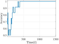
(a) Finite-time community recovery. The recovery is achieved after $t=383$.

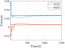
(b) Convergence of the interaction estimator. The solid (dashed) lines are true values (estimates).

Figure 2: Performance of Algorithm 1.

See Appendix G. $\Box$

Remark 21.

This result provides a sample complexity characterization for recovering community from a single trajectory. Multiple-trajectory sample complexity is investigated by [4, 5, 6]. The parameter $\delta$ reflects the combined effect of the cardinality of stubborn and regular agents and the interaction probabilities. $c_{\bar{A}}$ captures the “speed” of information diffusion, and increases with $\rho(\bar{A})$. $c_{n_{r}}$ depends on the number of regular agents. $c_{s}$ increases with the range of the states and decreases with the difference of averaged stubborn states in different communities, and $c_{w}$ measures the difference between interaction probabilities within and between communities. Smaller $\delta$, $c_{\bar{A}}$, $n_{r}$, and $\max\{|\underline{s}|,|\bar{s}|\}$ would make the recovery easier, and so would larger $c_{w}$ and $|n_{s1}\mathbf{1}^{T}_{n_{s2}}\mathbf{x}^{s2}-n_{s2}\mathbf{1}^{T}_{n_{s1}}\mathbf{x}^{s1}|$. For the gossip model over a graph sampled from an SBM, Example 1 indicates that the algorithm can recover most of the community labels, which is illustrated in Section 6.

We have the following result for the convergence rate of the interaction estimator. It shows that the convergence rate also depends on the model parameters, and a large enough step-size parameter $a$ ensures that the rate can achieve $O(1/\sqrt{t})$.

Theorem 22.

(Convergence rate) 
Under the conditions of Theorem 16, it holds for $d_{0}\in[0,\min\{1/2,a|\eta|\})$ that

$$(\hat{w}_{s}(t)-w_{s},\hat{w}_{d}(t)-w_{d})=o(t^{-d_{0}}),\text{ a.s.},$$

where $a>0$ is the step-size parameter given in Algorithm 1, $\eta=(w_{s}n_{2}+w_{d}n_{1})(n_{s1}\mathbf{1}^{T}_{n_{s2}}\mathbf{x}^{s2}-n_{s2}\mathbf{1}^{T}_{n_{s1}}\mathbf{x}^{s1})/$ $(\delta n_{1}n_{2})$, and $\delta$ is given in Proposition 10.

See Appendix H. $\Box$

Remark 23.

In the theorem, $\eta$ increases with the combined effect of the number of agents and the interaction probabilities (i.e., $(w_{s}n_{2}+w_{d}n_{1})/\delta$) and with the disagreement of stubborn agents, and decreases with the cardinality of each community. When $a\geq 1/(2|\eta|)$, the estimator achieves its optimal rate. Larger $\eta$ provides a wider selection range. Simulation in Section 6 shows that the algorithm using a trajectory from the gossip model over an SBM can estimate the ratio of the link probabilities.

6 Numerical Simulation

This section illustrates the performance of Algorithm 1, conducts an algorithm comparison, and applies Algorithm 1 to the SBM case and a real network.

To illustrate the performance of Algorithm 1 under Assumptions 4-14, consider a network consisting of twelve agents. The two communities both have five regular agents and one stubborn agent. Set interaction probabilities be $w_{s}=5/186$ and $w_{d}=~{}1/186$. The stubborn agent in community $1$ (resp. community $2$) has state $1$ (resp. $-1$). The initial states of regular agents are drawn from uniform distribution on $(-1,1)$. The averaging weight is set to be $q=1/2$ in all experiments. Fig. 2(a) shows that Algorithm 1 recovers the communities in finite time, where the accuracy at time $t$ is defined by $\frac{1}{n}(\max_{\sigma\in S_{2}}\{\sum_{i=1}^{n}\mathbb{I}_{[\sigma(\hat{\mathcal{C}}(i,t))=\mathcal{C}(i)]}\})\in[0,1]$. Here $\sigma:\{1,2\}\to\{1,2\}$ is a permutation function (to prevent a reverse distribution of labels), $S_{2}$ is the group of permutations on $\{1,2\}$, $\mathcal{C}(i)$ is agent $i$’s community label, $\hat{\mathcal{C}}(i,t)$ is the estimate of agent $i$’s label at time $t$, and $n=12$. Consistency of the interaction estimator with step-size parameter $a=1$ is demonstrated in Fig. 2(b). These results validate Theorem 16.

We now show the sample complexity of the community recovery (Theorem 20) and compare the recovery step with the $k$-means, $k$-means++ [35], and spectral clustering methods [12]. This experiment considers the gossip model under Assumptions 4-14 with $n=400$, $n_{1}=150$, and $n_{s1}=n_{s2}=8$. Let $w_{s}/w_{d}=5$ and solve the two parameters from (6). Let stubborn agents in community $1$ (resp. community $2$) have state $1$ (resp. $-1$), and generate the initial states of other agents from uniform distribution on $(-1,1)$. By running the algorithms for $200$ times, we obtain the relative frequency that the algorithms recover all community labels, defined by $p_{t}:=(\sum\nolimits_{k=1}^{N}\max_{\sigma\in S_{2}}\{\mathbb{I}_{\left[\sigma(\hat{\mathcal{C}}_{k}(i,t))=\mathcal{C}(i),\forall i\in\mathcal{V}\right]}\})/N$, where $N=200$ and $\hat{\mathcal{C}}_{k}(i,t)$ is the estimate of agent $i$’s label at time $t$ in the $k$-th run. After computing the time average $S^{r}(t)$, we use $k$-means and $k$-means++ with $k=2$ instead of Line 4 of Algorithm 1, to recover communities. To implement the spectral clustering method, assume that edge activation is known, and use the activation information to estimate the interaction probability matrix $W$. Applying spectral clustering to estimates of $W$ obtains community estimates.

Fig. 3 shows that the probabilities of unsuccessful community recovery of all approaches tends to zero exponentially over time. The spectral clustering method performs much better than other algorithms, because it directly uses interaction information, but the required time is still of the same order as the other algorithms. The $k$-means and $k$-means++ methods perform similarly to each other, and also similarly to Algorithm 1. This observation indicates that the major challenge of the considered problem is how to use agent states to recover communities without topological information.

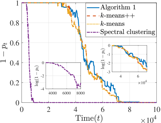
Figure 3: Performance comparison of four methods.

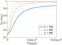
(a) Averaged accuracy of community recovery for each SBM.

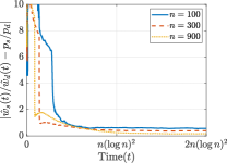
(b) Median of estimation error of $p_{s}/p_{d}$ for each SBM.

Figure 4: Performance of Algorithm 1 using trajectories of the gossip model over sampled graphs from SBMs with $n=100,300,900$.

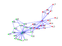
(a) The community structure of Zachary’s karate club network. Red squares and green triangles show two communities.

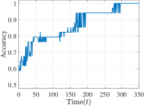
(b) Accuracy of community recovery of Algorithm 1 for the gossip model over Zachary’s karate club network.

Figure 5: Numerical experiment over Zachary’s karate club network.

We now consider the case where trajectories of the gossip model over graphs sampled from SBMs are given to Algorithm 1. We use three SBMs with size $n=100,300,900$ and with two equal-sized communities ($\nu_{1}=\nu_{2}=0.5$). Set $n_{r1}=n_{r2}=0.45n$, and $n_{s1}=n_{s2}=0.05n$. Let the link probability in the same community be $p_{s}=(\log n)^{2}/n$ and the link probability between different communities be $p_{d}=(\log n)/n$. For each SBM, we generate $20$ graph samples. For each graph sample, we run Algorithm 1 for $20$ times. Regular states are generated the same as earlier and stubborn agents in community $1$ (resp. community $2$) have state $1$ (resp. $-1$). Fig. 4(a) shows that Algorithm 1 has high community recovery accuracy, increasing with $n$. This phenomenon results from the concentration discussed in Example 1. Algorithm 1 outputs $\hat{w}_{s}(t)$ and $\hat{w}_{d}(t)$ as estimates of the two distinct non-zero values of $\mathbb{E}\{\mathcal{W}\}/\mathbb{E}\{\alpha\}$. Note that $[cp_{s},cp_{d}]$ defines the same $\mathbb{E}\{\mathcal{W}\}/\mathbb{E}\{\alpha\}$ for all $c>0$, so we can only estimate the ratio $p_{s}/p_{d}$ without knowing the expected number of edges of the SBM. Fig. 4(b) shows that the median of the estimation error for trajectory samples from each SBM is close to zero and decreases with $n$.

Zachary’s karate club network [36], presented in Fig. 5(a), is used to demonstrate an application of Algorithm 1. An edge represents frequent interaction between the two agents. The strength of interactions between agents is modeled by a weighted adjacency matrix (see matrix $C$ in [36]). A conflict between agents $1$ and $34$ results in a fission of the club. In the experiment, we assume that only the opinions can be observed, instead of interactions between agents. The process is modeled by the gossip model with stubborn agents. Agents $1$ and $34$ are set to be stubborn agents holding different opinions. In addition, one edge in Fig. 5(a) is selected at each time with a probability proportional to interaction strength given in [36]. The goal is to partition the agents into communities based on only state observations. Note that the network structure departures from our assumptions, but the result shown in Fig. 5(b) indicates that our algorithm can finally recover the community structure as time increases, without topological and interaction information.

7 Conclusion and Future Work

In this paper, we developed a joint algorithm to recover the community structure and to estimate the interaction probabilities for gossip opinion dynamics. It was proved that the community recovery is achieved in finite time, and the interaction estimator converges almost surely. We analyzed the sample complexity of the recovery and convergence rate of the estimator. Future work includes to study the case where all regular agents have the same stationary expectation, and to analyze the community detection problem for dynamics over the SBM.

This work was supported by Knut & Alice Wallenberg Foundation, Swedish Research Council, and National Natural Science Foundation of China (Grant No. 11931018).

Appendix

Appendix A Proof of Example 1

In this section, we prove the inequality given in Example 1. We need the following two results, whose proofs can be found in Sections 2.3 and 4.5 of [37], respectively.

Lemma 24 (Chernoff inequality).

Let $X=\sum_{i=1}^{n}X_{i}$, where $X_{i}$ are independent Bernoulli random variables with expectation $p_{i}$, and let $\mu:=\mathbb{E}\{X\}=\sum_{i=1}^{n}p_{i}$. Then for all $\delta\in(0,1)$,

$$\mathbb{P}\{|X-\mu|\geq\delta\mu\}\leq 2e^{-\mu\delta^{2}/3},$$

and for all $a>\mu$,

$$\mathbb{P}\{X\geq a\}\leq e^{-\mu}\Big{(}\frac{e\mu}{a}\Big{)}^{a}.$$

Lemma 25 (Matrix Bernstein inequality).

Let $Y_{i}$, $1\leq i\leq k$, be independent $n$-dimensional random symmetric matrices such that $\|Y_{i}-\mathbb{E}\{Y_{i}\}\|\leq C_{0}$. Denote $Y:=\sum_{i=1}^{k}Y_{i}$. Then for all $a>0$,

$$\mathbb{P}\{\|Y-\mathbb{E}\{Y\}\|>a\}\leq 2n\exp\bigg{\{}\frac{-a^{2}}{2v^{2}+2C_{0}a/3}\bigg{\}},$$

where $v^{2}=\|\sum_{i=1}^{k}\textup{var}(Y_{i})\|$.

Now we prove the inequality given in Example 1. For two sequences of real numbers $\{a_{k}\}$ and $\{b_{k}\}$ with $b_{k}\not=0$, $k\geq 1$, denote $a_{k}\sim b_{k}$, if $\lim_{k\to\infty}a_{k}/b_{k}=1$. Hence for $\alpha=\sum_{i=1}^{n}\sum_{j=i+1}^{n}a_{ij}$, it holds that

$$\mathbb{E}\{\alpha\} =\Big{[}\frac{1}{2}p_{s}\Big{(}\nu_{1}^{2}+\nu_{2}^{2}-\frac{\nu_{1}}{n}-\frac{\nu_{2}}{n}\Big{)}+p_{d}\nu_{1}\nu_{2}\Big{]}n^{2}$$

$$\sim\Big{[}\frac{1}{2}p_{s}\Big{(}\nu_{1}^{2}+\nu_{2}^{2}\Big{)}+p_{d}\nu_{1}\nu_{2}\Big{]}n^{2}.$$

Note that

$$\bigg{\|}\tilde{W}-\frac{\mathbb{E}\{\mathcal{A}\}}{\mathbb{E}\{\alpha\}}\bigg{\|}$$

$$=\bigg{\|}\frac{\mathcal{A}}{\alpha}-\frac{\mathbb{E}\{\mathcal{A}\}}{\mathbb{E}\{\alpha\}}\bigg{\|}$$

$$\leq\bigg{\|}\frac{\mathcal{A}}{\alpha}\bigg{\|}\bigg{|}1-\frac{\alpha}{\mathbb{E}\{\alpha\}}\bigg{|}+\bigg{\|}\frac{\mathcal{A}-\mathbb{E}\{\mathcal{A}\}}{\mathbb{E}\{\alpha\}}\bigg{\|}.$$

We first bound terms related to $\alpha$. Setting $\delta=1/2$ and we obtain from Lemma 24 that

$$\mathbb{P}\{\alpha-\mathbb{E}\{\alpha\}\leq-\mathbb{E}\{\alpha\}/2\}$$

$$\leq 2\exp\{-\mathbb{E}\{\alpha\}/12\}$$

$$\sim 2\exp\{-[(\nu_{1}^{2}+\nu_{2}^{2})p_{s}+2\nu_{1}\nu_{2}p_{d}]n^{2}/24\}.$$

Utilizing Lemma 24 again with $\delta=1/\sqrt{n}$, we have that

$$\mathbb{P}\{|\alpha-\mathbb{E}\{\alpha\}|\geq\mathbb{E}\{\alpha\}/\sqrt{n}\}$$

$$=\mathbb{P}\bigg{\{}\bigg{|}\frac{\alpha}{\mathbb{E}\{\alpha\}}-1\bigg{|}\geq\frac{1}{\sqrt{n}}\bigg{\}}$$

$$\leq 2e^{-\mathbb{E}\{\alpha\}/(3n)}$$

$$\sim 2n^{-[(\nu_{1}^{2}+\nu_{2}^{2})p_{s}+2\nu_{1}\nu_{2}p_{d}]n/(6\log n)}.$$

Now we decompose $\mathcal{A}-\mathbb{E}\{\mathcal{A}\}$ as the sum of independent random matrices $\sum_{i=1}^{n}\sum_{j=i+1}^{n}Y_{ij}$ where $Y_{ij}:=(a_{ij}-\mathbb{E}\{a_{ij}\})(E_{ij}+E_{ji})$. Thus, $\|Y_{ij}\|\leq 2$ and $\textup{var}(Y_{ij})=\mathbb{E}\{Y_{ij}^{2}\}=(\mathbb{E}\{a_{ij}\}-(\mathbb{E}\{a_{ij}\})^{2})(E_{ii}+E_{jj})$, where $E_{ij}=\mathbf{e}_{i}\mathbf{e}_{j}^{T}$. Hence

$$v^{2} =\bigg{\|}\sum_{i=1}^{n}\sum_{j=i+1}^{n}\textup{var}(Y_{ij})\bigg{\|}$$

$$\leq n\max\{\nu_{1}p_{s}+\nu_{2}p_{d},\nu_{1}p_{d}+\nu_{2}p_{s}\}$$

$$=:\beta_{1}.$$

Therefore, from Lemma 25, it follows that

$$\mathbb{P}\{\|\mathcal{A}-\mathbb{E}\{\mathcal{A}\}\|>a\}\leq 2n\exp\bigg{\{}\frac{-a^{2}}{2\beta_{1}+4a/3}\bigg{\}}.$$

Let $a=C_{1}\sqrt{\beta_{1}\log n}$ for some constant $C_{1}$, and it holds that

$$\mathbb{P}\{\|\mathcal{A}-\mathbb{E}\{\mathcal{A}\}\|>C_{1}\sqrt{\beta_{1}\log n}\}$$

$$\leq 2n\exp\bigg{\{}\frac{-C_{1}^{2}\beta_{1}\log n}{2\beta_{1}+4C_{1}\sqrt{\beta_{1}\log n}/3}\bigg{\}}$$

$$=2n^{1-C_{1}^{2}/(2+4C_{1}\sqrt{\log n/\beta_{1}}/3)}.$$

The right-hand side of the preceding equation tends to zero as $n\to\infty$ when the constant $C_{1}$ is large enough and $\log n/n=O(\max\{p_{s},p_{d}\})$.

Finally, we need a bound for $\|\mathcal{A}\|$. Note that $\|\mathcal{A}\|\leq\|\mathbb{E}\{\mathcal{A}\}\|+\|\mathcal{A}-\mathbb{E}\{\mathcal{A}\}\|$. Since we have already bound the second term, it suffices to study the spectrum of $\mathbb{E}\{\mathcal{A}\}$. Observe that $\mathbb{E}\{\mathcal{A}\}+p_{s}I_{n}$ has rank $2$ and its two eigenvectors corresponding to the nonzero eigenvalues are $[\mathbf{1}_{\nu_{1}n}^{T}~{}\mathbf{1}_{\nu_{2}n}^{T}]^{T}$ and $[\mathbf{1}_{\nu_{1}n}^{T}~{}-\mathbf{1}_{\nu_{2}n}^{T}]^{T}$. We can compute nonzero eigenvalues and obtain the upper bound of their absolute values as follows

$$\frac{n}{2}\Big{|}p_{s}\pm\sqrt{(1-4\nu_{1}\nu_{2})p_{s}^{2}+4\nu_{1}\nu_{2}p_{d}^{2}}\Big{|}$$

$$\leq\frac{n}{2}\Big{(}p_{s}+\sqrt{(1-4\nu_{1}\nu_{2})p_{s}^{2}+4\nu_{1}\nu_{2}p_{d}^{2}}\Big{)}=:\beta_{2}.$$

So $\|\mathbb{E}\{\mathcal{A}\}\|\leq\beta_{2}+p_{s}$. To sum up, it holds that

$$\bigg{\|}\tilde{W}-\frac{\mathbb{E}\{\mathcal{A}\}}{\mathbb{E}\{\alpha\}}\bigg{\|}$$

$$\leq\bigg{\|}\frac{\mathcal{A}}{\alpha}\bigg{\|}\bigg{|}1-\frac{\alpha}{\mathbb{E}\{\alpha\}}\bigg{|}+\bigg{\|}\frac{\mathcal{A}-\mathbb{E}\{\mathcal{A}\}}{\mathbb{E}\{\alpha\}}\bigg{\|}$$

$$\leq\frac{2(C_{1}\sqrt{\beta_{1}\log n}+\beta_{2}+p_{s})}{\mathbb{E}\{\alpha\}\sqrt{n}}+\frac{C_{1}\sqrt{\beta_{1}\log n}}{\mathbb{E}\{\alpha\}}$$

$$\leq\frac{C}{n},$$

with probability

$$1-2\exp\{-[(\nu_{1}^{2}+\nu_{2}^{2})p_{s}+2\nu_{1}\nu_{2}p_{d}]n^{2}/24\}$$

$$-2n^{-[(\nu_{1}^{2}+\nu_{2}^{2})p_{s}+2\nu_{1}\nu_{2}p_{d}]n/(6\log n)}$$

$$-4n^{1-C_{1}^{2}/(2+4C_{1}\sqrt{\log n/\beta_{1}}/3)}\to 1,$$

as $n\to\infty$, if $\log n/n=O(\min\{p_{s},p_{d}\})$. $\Box$

Appendix B Result on multiple-community case

In this section, we provide a result on the expression of $(I-\bar{A})^{-1}\bar{B}$ in the multiple-community case without proof, as a counterpart of Proposition 10, and briefly discuss how to generalize Algorithm 1 to the multiple-community case.

B.1 Notation

Let $[n]:=\{1,2,\dots,n\}$, where $n$ is a positive integer. Denote the set consisting of all ordered $d$-tuples from the set $[n]$ by $[n]^{d}_{<}$, namely,

$$[n]^{d}_{<}:=\{(i_{1},\dots,i_{d})\in[n]^{d}:1\leq i_{1}<i_{2}<\cdots<i_{d}\leq n\},$$

where $[n]^{d}$ is the $d$-fold Cartesian product of $[n]$. More generally, for a set $\mathcal{S}$ containing finite number of distinct positive integers, we denote $\prescript{}{-i}{\mathcal{S}}:=\mathcal{S}\setminus\{i\}$ for $i\in\mathcal{S}$, and use $\mathcal{S}^{d}_{<}$ to represent the set consisting of all ordered $d$-tuples from the set $\mathcal{S}$, i.e.,

$$\mathcal{S}^{d}_{<}:=\{(i_{1},\dots,i_{d})\in\mathcal{S}^{d}:$$

$$\qquad\min\mathcal{S}\leq i_{1}<i_{2}<\cdots<i_{d}\leq\max\mathcal{S}\},$$

where $\min\mathcal{S}$ and $\max\mathcal{S}$ are the minimum and maximum of $\mathcal{S}$. Specifically, let $\prescript{}{-i}{[n]}:=[n]\setminus\{i\}$ for $i\in[n]$, and $\prescript{}{-i}{[n]}^{d}_{<}$ stands for the set consisting of all ordered $d$-tuples from $\prescript{}{-i}{[n]}$.

B.2 Result and discussion

We consider the scenario where the agents can be partitioned into multiple groups $\mathcal{V}_{1},\dots,\mathcal{V}_{K}$ (i.e., $\mathcal{V}=\cup_{k=1}^{K}\mathcal{V}_{k}$ and $\mathcal{V}_{k}\cap\mathcal{V}_{l}=\emptyset$ for all $k,l\in[K]$). To ease notation, we assume that $\mathcal{V}_{1}=\{1,\dots,n_{1}\}$, $\mathcal{V}_{2}=\{n_{1}+1,\dots,n_{1}+n_{2}\}$, $\dots$, $\mathcal{V}_{K}=\{1+\sum_{i=1}^{K-1}n_{i},\dots,n_{K}+\sum_{i=1}^{K-1}n_{i}\}$ with $n_{i}:=|\mathcal{V}_{i}|$, $i\in[K]$, and $\sum_{i=1}^{K}n_{k}=n$. Also, sort regular and stubborn agents in each community in the following way, $\mathcal{V}_{ri}=\{1+\sum_{j=1}^{i-1}n_{j},\dots,n_{ri}+\sum_{j=1}^{i-1}n_{j}\}$, $\mathcal{V}_{si}=\{1+n_{ri}+\sum_{j=1}^{i-1}n_{j},\dots,n_{i}+\sum_{j=1}^{i-1}n_{j}\}$, $i\in[K]$. Here, $\mathcal{V}_{ri}$ (resp. $\mathcal{V}_{si}$) is the set of regular (resp. stubborn) agents in community $i$. Let $n_{ri}:=|\mathcal{V}_{ri}|$ and $n_{si}:=|\mathcal{V}_{si}|$. Finally, denote the cardinality of regular and stubborn agents by $n_{r}:=|\mathcal{V}_{r}|=\sum_{i=1}^{K}n_{ri}$ and $n_{s}:=|\mathcal{V}_{s}|=\sum_{i=1}^{K}n_{si}$ respectively. Assumptions in the multiple-community case, similar to Assumption 4, are summarized as follows.

Assumption 26.

(1.a) The agent set $\mathcal{V}$ consists of $K$ communities with $K\geq 2$, $n_{i}>0$, $i\in[K]$, and $\sum_{i=1}^{K}n_{i}=n$.
(1.b) All communities have regular agents, namely, $1\leq n_{ri}\leq n_{i}$, $i\in[K]$.
(2) The within-group and inter-group interaction probabilities are $w_{s},w_{d}>0$, respectively, with $w_{s}\not=w_{d}$, and

$$\left(\sum_{i=1}^{K}n_{i}(n_{i}-1)\right)w_{s}+\left(\sum_{i=1}^{K}\sum_{j\not=i}n_{i}n_{j}\right)w_{d}=2.$$

(3) $X(0)$ is deterministic. It holds that $X^{r}(0)\in\mathcal{S}$, with

$$\mathcal{S}:=\{x\in\mathbb{R}^{n_{r}}:x_{i}\in[\underline{s},\overline{s}],1\leq i\leq n_{r}\},$$

where $\underline{s}:=\min_{1\leq i\leq n_{s}}\{\mathbf{x}_{i}^{s}\}$, $\overline{s}:=\max_{1\leq i\leq n_{s}}\{\mathbf{x}_{i}^{s}\}$, $\mathbf{x}^{s}:=X^{s}(0)=[(\mathbf{x}^{s1})^{T}~{}(\mathbf{x}^{s2})^{T}~{}\cdots~{}(\mathbf{x}^{sK})^{T}]^{T}$ is the stubborn state vector, and $\mathbf{x}^{sk}$ is the vector for the community $k$, $k\in[K]$.

The following proposition generalizes Proposition 10 to the multiple-community case under Assumption 26. The proof directly follows from the inverse formula of block matrices [38] and is omitted.

Proposition 27.

Suppose that Assumption 26 holds and there exists at least one stubborn agent in the network (i.e., $n_{r}<n$). Then $(I-\bar{A})^{-1}$ exists, and it holds that

$$(I-\bar{A})^{-1}=(1-q)^{-1}\begin{bmatrix}\tilde{A}^{(11)}&\tilde{A}^{(12)}&\cdots&\tilde{A}^{(1K)}\\ \tilde{A}^{(21)}&\ddots&\cdots&\vdots\\ \vdots&\cdots&\ddots&\tilde{A}^{(K-1,K)}\\ \tilde{A}^{(K1)}&\cdots&\tilde{A}^{(K,K-1)}&\tilde{A}^{(KK)}\end{bmatrix},$$

where

$$\tilde{A}^{(ii)}=\frac{1}{w_{s}n_{i}+w_{d}\sum_{j\not=i}n_{j}}$$

$$\bigg{[}I_{n_{ri}}-\frac{1}{n_{ri}}\bigg{(}1-\frac{d_{A}(\prescript{}{-i}{[K]})}{d_{A}([K])}\bigg{)}\mathbf{1}_{n_{ri},n_{ri}}\bigg{]},~{}i\in[K],$$

$$\tilde{A}^{(ij)}$$

$$=\frac{w_{d}e_{A}([K]\setminus\{i,j\})\mathbf{1}_{n_{ri},n_{rj}}}{(w_{s}n_{i}+w_{d}\sum_{k\not=i}n_{k})(w_{s}n_{j}+w_{d}\sum_{k\not=j}n_{k})d_{A}([K])},$$

$$~{}i,j\in[K],~{}i\not=j.$$

Here

$$d_{A}(\mathcal{S}) =-\sum_{p=0}^{|\mathcal{S}|}\sum_{(j_{1},\dots,j_{p})\in\mathcal{S}^{p}_{<}}\bigg{[}(w_{d}-w_{s})^{p-1}$$

$$(w_{s}+(p-1)w_{d})\prod_{l=1}^{p}\bigg{(}\frac{n_{r,j_{l}}}{w_{s}n_{j_{l}}+w_{d}\sum_{k\not=j_{l}}n_{k}}\bigg{)}\bigg{]},$$

$$e_{A}(\mathcal{S}) =\prod_{p\in\mathcal{S}}\bigg{(}1+\frac{(w_{d}-w_{s})n_{rp}}{w_{s}n_{p}+w_{d}\sum_{j\not=p}n_{j}}\bigg{)},$$

where $\mathcal{S}$ is a set consisting of finite number of distinct positive integers, for $p=0$ we define the term $\sum_{(j_{1},\dots,j_{p})\in\mathcal{S}^{p}_{<}}\prod_{l=1}^{p}(n_{r,j_{l}}/(w_{s}n_{j_{l}}+w_{d}\sum_{k\not=j_{l}}n_{k}))=1$, and $d_{A}(\emptyset)=e_{A}(\emptyset)=1$. In addition,

$$(I-\bar{A})^{-1}\bar{B}=\begin{bmatrix}\tilde{B}^{(11)}&\tilde{B}^{(12)}&\cdots&\tilde{B}^{1K}\\ \tilde{B}^{(21)}&\ddots&\cdots&\vdots\\ \vdots&\cdots&\ddots&\tilde{B}^{(K-1,K)}\\ \tilde{B}^{(K1)}&\cdots&\tilde{B}^{(K,K-1)}&\tilde{B}^{(KK)}\end{bmatrix},$$

where

$$\tilde{B}^{ii} =\frac{1}{n_{ri}}\bigg{(}\frac{d_{A}(\prescript{}{-i}{[K]})}{d_{A}([K])}-1\bigg{)}\mathbf{1}_{n_{ri},n_{si}},~{}i\in[K],$$

$$\tilde{B}^{ij} =\frac{w_{d}e_{A}([K]\setminus\{i,j\})}{(w_{s}n_{i}+w_{d}\sum_{k\not=i}n_{k})d_{A}([K])}\mathbf{1}_{n_{ri},n_{sj}},$$

$$i,j\in[K],~{}i\not=j.$$

Remark 28.

The above proposition provides a parallel result of Proposition 10, and shows that $(I-\bar{A})^{-1}\bar{B}$ has a block structure and hence so does $\mathbf{x}^{r}$. The developed framework in the current paper indicates that studying a condition similar to Assumption 12 would be the key to addressing the problem in the general case, but such condition would be more complex and the investigation of it is beyond the scope of this paper. Note that it is possible to generalize Algorithm 1 to the multiple-community case by examining the structure of $\mathbf{x}^{r}$ more carefully, and the techniques we developed in the current paper would contribute to the analysis of the generalized algorithm.

Appendix C Some results on stochastic approximation

In this section we introduce some results, which are used throughout the later appendices, on a linear stochastic approximation algorithm. Consider deterministic matrices $H(t),H\in\mathbb{R}^{l\times l}$ and random vectors $z(t),e(t),v(t)\in\mathbb{R}^{l}$, and define the following linear recursion,

$$z(t+1) =z(t)+a(t)H(t)z(t)+a(t)(e(t)+v(t))$$ (14)

The following results follow from Lemma 3.1.1 and Theorem 3.1.1 of [39].

Proposition 29.

Assume $a(t)$ is such that $a(t)>0$, $a(t)\to 0$ as $t\to\infty$, $\sum_{t=1}^{\infty}a(t)=\infty$, and

$$a^{-1}(t+1)-a^{-1}(t)\to\alpha\geq 0.$$ (15)

If $\sum_{t=1}^{\infty}a(t)^{1-d}e(t)<\infty$ and $v(t)=o(a(t)^{d})$ as $t\to\infty$ for some $d\in[0,1/2)$, $H(t)\to H$, and $H+\alpha dI$ is stable (all its eigenvalues are with negative real parts), then $z(t)/a(t)^{d}\to 0$.

Appendix D Proof of Theorem 8

From Theorem 2.1 of [40] we have the following stability result for Markov chains.

Proposition 30.

Consider a Markov chain on $\mathbb{R}^{n}$, defined by

$$Y(t+1)=A(t)Y(t)+U(t),\quad t\in\mathbb{N},$$

where $\{[A(t)~{}U(t)],t\in\mathbb{N}\}$ is a sequence of i.i.d. random matrices taking values in $\mathbb{R}^{n\times(n+1)}$, such that $\mathbb{E}\{\log^{+}\|A(t)\|\}<\infty$ and $\mathbb{E}\{\log^{+}\|U(t)\|\}<\infty$ ($x^{+}=x$ if $x>0$, $x^{+}=0$ if $x\leq 0$). Suppose that

$$\inf_{t>0}\frac{1}{t}\mathbb{E}\left\{\log\Big{\|}\overleftarrow{\Phi}_{A}(0,t-1)\Big{\|}\right\}<0,$$

where $\overleftarrow{\Phi}_{A}(s,t):=A(s)\cdots A(t)$ for $0\leq s\leq t$, and $\overleftarrow{\Phi}_{A}(s,t)=I$ for $s>t$. In addition, the only invariant subspace of $\mathbb{R}^{n}$ is itself, where an invariant subspace is a linear subspace $L\subset\mathbb{R}^{n}$ such that $\mathbb{P}\{Y(1)\in L|Y(0)=y\}=1$ for all $y\in L$. Then the infinite random series $Y^{*}=\sum_{j=0}^{\infty}\overleftarrow{\Phi}_{A}(0,j-1)$ $U(j)$ converges a.s., and its distribution is the unique stationary distribution of the Markov chain $\{Y(t)\}$.

We also need the following lemma for substochastic matrices to establish Corollary 7, which will be used in the proof of Theorem 8.

Lemma 31.

Consider a substochastic matrix $A=[a_{ij}]\in\mathbb{R}^{n\times n}$. If for every row $i$, $1\leq i\leq n$, there exists an integer $j,~{}1\leq j\leq n$, satisfying that the sum of $j$-th row less than one, and a sequence of distinct integers $k_{1}=i,~{}k_{2},\dots,~{}k_{m}=~{}j,~{}1\leq m\leq n$, such that $a_{k_{1}k_{2}}a_{k_{2}k_{3}}\cdots a_{k_{m-1}k_{m}}>0$, then $\rho(A)<1$.

From Theorem 8.3.1 of [41], we know that there is a nonnegative nonzero vector $x\in\mathbb{R}^{n}$ such that

$$x^{T}A=\rho(A)x^{T}.$$

Let $\mathcal{T}:=\{1\leq i\leq n:x_{i}>0\}$, then

$$\rho(A)\sum\nolimits_{i\in\mathcal{T}}x_{i} =\sum\nolimits_{i\in\mathcal{T}}(A^{T}x)_{i}$$

$$=\sum\nolimits_{i\in\mathcal{T}}\Big{(}\sum\nolimits_{1\leq j\leq n}a_{ji}x_{j}\Big{)}$$

$$=\sum\nolimits_{1\leq j\leq n}x_{j}\sum\nolimits_{i\in\mathcal{T}}a_{ji}$$

$$=\sum\nolimits_{j\in\mathcal{T}}x_{j}\sum\nolimits_{i\in\mathcal{T}}a_{ji}.$$

There must exists $j\in\mathcal{T}$ such that $\sum_{i\in\mathcal{T}}a_{ji}<1$. Otherwise, $\sum_{i\in\mathcal{T}}a_{ji}=1$ for all $j\in\mathcal{T}$ and $\mathcal{T}\subsetneqq\{1,\dots,n\}$ by assumption, which means that $a_{jk}=0$, for all $k\not\in\mathcal{T}$. This contradicts with the assumption. So $\rho(A)\sum_{i\in\mathcal{T}}x_{i}<\sum_{j\in\mathcal{T}}x_{j}$, and $\rho(A)<1$. $\Box$

Proof of Theorem 8:

We use Proposition 30 and Corollary 7 to verify the first part of (i). Note that

$$\mathbb{E}\Big{\{}\Big{\|}\overleftarrow{\Phi}_{A}(0,t)\Big{\|}_{1}\Big{\}}$$

$$=\mathbb{E}\Big{\{}\underset{1\leq j\leq n}{\text{max}}\sum\nolimits_{1\leq i\leq n}\Big{|}\Big{[}\overleftarrow{\Phi}_{A}(0,t)\Big{]}_{ij}\Big{|}\Big{\}}$$

$$\leq\sum\nolimits_{1\leq j\leq n}\sum\nolimits_{1\leq i\leq n}\mathbb{E}\Big{\{}\Big{|}\Big{[}\overleftarrow{\Phi}_{A}(0,t)\Big{]}_{ij}\Big{|}\Big{\}}$$

$$\leq n\Big{\|}\mathbb{E}\Big{\{}\overleftarrow{\Phi}_{A}(0,t)\Big{\}}\Big{\|}_{\infty}$$

$$\leq\gamma n(t+1)^{n-1}\rho(\bar{A})^{t+1},$$ (16)

for some constant $\gamma>0$, where the last equality follows from the Jordan canonical decomposition. Thus from Jensen’s inequality, we have that

$$\inf_{t>0}\frac{1}{t}\mathbb{E}\Big{\{}\log\Big{\|}\overleftarrow{\Phi}_{A}(0,t-1)\Big{\|}_{1}\Big{\}}$$

$$\leq\lim_{t\to\infty}\frac{\log(\gamma nt^{n-1}\rho(\bar{A})^{t})}{t}=\log\rho(\bar{A})<0,$$

from Corollary 7.

Assumption (iii), the assumption for the existence of stubborn agents, and update rule (1) ensure that $\mathbb{R}^{n}$ is the only invariant subspace of itself. So let $U(t):=B(t)X^{s}(t)$, and it follows from Proposition 30 that $X^{r}_{*}:=\sum_{j=0}^{\infty}\overleftarrow{\Phi}_{A}(0,j-1)U(j)$ converges a.s., and its distribution $\pi$ is the unique stationary distribution of $\{X^{r}(t)\}$. In addition, from Markov inequality and (16),

$$\mathbb{P}\Big{\{}\Big{\|}\overleftarrow{\Phi}(0,t-1)\Big{\|}_{1}\geq\varepsilon\Big{\}}\leq\varepsilon^{-1}\gamma nt^{n-1}\rho(\bar{A})^{t}.$$

So by Borel-Cantelli lemma, $\overleftarrow{\Phi}_{A}(0,t)X^{r}(0)$ converges to zero a.s. Hence $\overleftarrow{X}^{r}(t):=\overleftarrow{\Phi}_{A}(0,t-1)X^{r}(0)+\sum_{j=0}^{t-1}\overleftarrow{\Phi}_{A}(0,j-1)U(j)$ converges a.s. to $X^{r}_{*}$. Since $\overleftarrow{X}^{r}(t)$ and $X^{r}(t)$ has the same distribution, we have that $X^{r}(t)\overset{\textup{d}}{\to}\pi$, as $t\to\infty$.

For (ii) of the theorem, since $|U(t)|<L$ for some positive $L>0$, by dominated convergence theorem, $\mathbb{E}\{X^{r}_{*}\}=\lim_{t\to\infty}\mathbb{E}\{\overleftarrow{X}^{r}(t)\}$. It follows that $\mathbb{E}\{X^{r}_{*}\}=\sum_{j=0}^{\infty}\bar{A}^{j}\bar{u}=(I-\bar{A})^{-1}\bar{u}$ from independence and $\rho(\bar{A})<1$, where $\bar{u}:=\mathbb{E}\{U(t)\}=\bar{B}\textbf{x}^{s}$. Finally, $X^{r}(t)$ and $\overleftarrow{X}^{r}(t)$ have the same distribution, so $\mathbb{E}\{X^{r}(t)\}=\mathbb{E}\{\overleftarrow{X}^{r}(t)\}$, and (9) holds.

To prove (iii), write

$$S^{r}(t+1)=S^{r}(t)-\frac{1}{t+1}S^{r}(t)+\frac{1}{t+1}X^{r}(t).$$

Using notations in Appendix C, let $z(t)=S^{r}(t)-\mathbf{x}^{r}$, $a(t)=1/(t+1)$, $H(t)\equiv H=-I$, $e(t)=X^{r}(t)-\mathbb{E}\{X^{r}(t)\}$, and $v(t)=\mathbb{E}\{X^{r}(t)\}-\mathbf{x}^{r}$. So from Proposition 29 in Appendix C, to show $z(t)\to 0$, it suffices to validate that $\sum_{t=1}^{\infty}a(t)e(t)<\infty$ and $v(t)\to 0$ as $t\to\infty$. The latter follows from (ii). Note that

$$\sum\nolimits_{t=1}^{\infty}a(t)e(t)$$

$$=\sum\nolimits_{t=1}^{\infty}a(t)(X^{r}(t)-\mathbb{E}\{X^{r}(t)\})$$

$$=\sum\nolimits_{t=1}^{\infty}a(t)(A(t-1)X^{r}(t-1)+U(t-1)$$

$$~{}-\bar{A}\mathbb{E}\{X^{r}(t-1)\}-\bar{u})$$

$$=\sum\nolimits_{t=1}^{\infty}a(t)(A(t-1)-\bar{A})X^{r}(t-1)$$

$$~{}+\sum\nolimits_{t=1}^{\infty}a(t)(U(t-1)-\bar{u})$$

$$~{}+\bar{A}\sum\nolimits_{t=1}^{\infty}a(t)(X^{r}(t-1)-\mathbb{E}\{X^{r}(t-1)\})$$

$$=\sum\nolimits_{t=1}^{\infty}a(t)(A(t-1)-\bar{A})X^{r}(t-1)$$

$$~{}+\sum\nolimits_{t=1}^{\infty}a(t)(U(t-1)-\bar{u})$$

$$~{}+\bar{A}\sum\nolimits_{t=0}^{\infty}a(t)(X^{r}(t)-\mathbb{E}\{X^{r}(t)\})$$

$$~{}+\bar{A}\sum\nolimits_{t=1}^{\infty}(a(t)-a(t-1))$$

$$\qquad\qquad(X^{r}(t-1)-\mathbb{E}\{X^{r}(t-1)\})$$ (17)

On the right side of the above equality, the first two terms are weighted sums of martingale difference sequences, and converge by Theorem B.6.1 of [39], and the last term converges since $X^{r}(t)$ is bounded and $a(t)-a(t-1)$ $=-1/t(t+1)$. Hence $\sum_{t=1}^{\infty}a(t)e(t)<\infty$ is obtained by combining the left side and the third term on the right together, and noting that $(I-\bar{A})^{-1}$ exists by Corollary 7.  $\Box$

Remark 32.

Note that, similar to the proof of Theorem 8 (iii), we are able to show that $\sum_{t=1}^{\infty}a(t)^{1-d}e(t)<\infty$, for all $d\in[0,1/2)$. Since $\mathbb{E}\{X^{r}(t)\}$ converges exponentially to $\mathbf{x}^{r}$, it holds that $v(t)=o(a(t)^{d})$ for all $d\in[0,1/2)$. Therefore, from Proposition 29, it follows that $(S^{r}(t)-\mathbf{x}^{r})/a(t)^{d}\to 0$ a.s., for all $d\in[0,1/2)$.

Appendix E Proof of Theorem 16

We know from (10) that $S^{r}(t)\to\mathbf{x}^{r}$ a.s., as $t\to\infty$, where $S^{r}(t)=[S^{r}_{i}(t)]_{1\leq i\leq n_{r}}$. That is, $S^{r}_{i}(t)\to\chi_{1}$ for $1\leq i\leq n_{r1}$ and $S^{r}_{i}(t)\to\chi_{2}$ for $n_{r1}+1\leq i\leq n_{r}$. Hence for $\varepsilon=|\chi_{1}-\chi_{2}|/(2n_{r}(n_{r}+1))$, there exists an integer-valued random variable $T$ such that for all $t>T$, $|S^{r}_{i}(t)-\chi_{1}|<\varepsilon$ for $1\leq i\leq n_{r1}$, and $|S^{r}_{i}(t)-\chi_{2}|<\varepsilon$ for $n_{r1}+1\leq i\leq n_{r}$. Since Assumption 12 ensures that $\chi_{1}\not=\chi_{2}$, we can assume that $\chi_{1}>\chi_{2}$. Consequently, from $n_{r1}\geq 1$ and $n_{r2}\geq 1$,

$$(\chi_{1}-\varepsilon)-\Big{(}\frac{n_{r1}\chi_{1}+n_{r2}\chi_{2}}{n_{r}}+n_{r}\varepsilon\Big{)} >0,$$

$$(\chi_{2}+\varepsilon)-\Big{(}\frac{n_{r1}\chi_{1}+n_{r2}\chi_{2}}{n_{r}}-n_{r}\varepsilon\Big{)} <0.$$

This fact means that $S^{r}_{i}(t)>\bar{s}^{r}(t)$ for $1\leq i\leq n_{r1}$ and $S^{r}_{i}(t)<\bar{s}^{r}(t)$ for $n_{r1}+1\leq i\leq n_{r}$, $\forall t>T$, which implies the finite-time convergence of the community recovery step, combined with Assumption 14.

Now we can assume that the true community has been recovered since this recovery step converges in finite time $T$. As a consequence, we know the community structure of all agents for $t>T$, and also the size of both communities (i.e., $n_{1}$ and $n_{2}$). In other words, $\hat{n}_{k}(t)=n_{k}$, $k=1,2$, $t>T$. Hence $\hat{w}_{s}(t)$ in Line $5$ of Algorithm 1 can be rewritten as follows for $t>T+1$,

$$\hat{w}_{s}(t)=\hat{w}_{s}(t-1)-\frac{a}{t}\text{sgn}(g(t))\Big{(}g(t)\hat{w}_{s}(t-1)+\frac{h_{2}(t)}{n_{1}n_{2}}\Big{)},$$ (18)

where $g(t)=h_{1}(t)-\frac{n_{1}^{2}+n_{2}^{2}-n_{1}-n_{2}}{2n_{1}n_{2}}h_{2}(t)$ and

$$h_{1}(t) =\frac{n_{s1}}{n_{r1}}\sum\nolimits_{i\in\mathcal{V}_{r1}}S^{r}_{i}(t)-\mathbf{1}_{n_{s1}}^{T}\mathbf{x}^{s1},$$

$$h_{2}(t) =\frac{n_{2}}{n_{r1}}\sum\nolimits_{i\in\mathcal{V}_{r1}}S^{r}_{i}(t)-\sum\nolimits_{i\in\mathcal{V}_{r2}}S^{r}_{i}(t)-\mathbf{1}_{n_{s2}}^{T}\mathbf{x}^{s2}.$$

In order to utilize Proposition 29 in Appendix C, let $z(t)=\hat{w}_{s}(t)-w_{s}$, $a(t)=a/(t+1)$, $H(t)=-|g(t+1)|$, and

$$v(t)=-\text{sgn}(g(t+1))\Big{(}\frac{h_{2}(t+1)}{n_{1}n_{2}}+g(t+1)w_{s}\Big{)}.$$

From the fact that (13) has a unique solution, it holds that $H(t)\to H:=-|\eta|<0$, where $\eta=$ $h_{1}^{*}-\frac{n_{1}^{2}+n_{2}^{2}-n_{1}-n_{2}}{2n_{1}n_{2}}h_{2}^{*}\not=0$ with $h_{1}^{*}=n_{s1}\chi_{1}-\mathbf{1}_{n_{s1}}^{T}\mathbf{x}^{s1}$ and $h_{2}^{*}=n_{2}\chi_{1}-n_{r2}\chi_{2}-\mathbf{1}_{n_{s2}}^{T}\mathbf{x}^{s2}$. Notice that

$$\frac{h_{2}(t)}{n_{1}n_{2}}+g(t)w_{s}$$

$$=h_{1}(t)w_{s}+\frac{h_{2}(t)}{2n_{1}n_{2}}(2-(n_{1}^{2}+n_{2}^{2}-n_{1}-n_{2})w_{s})$$

$$\to h_{1}^{*}w_{s}+\frac{h_{2}^{*}}{2n_{1}n_{2}}(2-(n_{1}^{2}+n_{2}^{2}-n_{1}-n_{2})w_{s}),$$

from (10), and this limit is $h_{1}^{*}w_{s}+h_{2}^{*}w_{d}=0$ by (13), implying $v(t)\to 0$. So the interaction estimator converges by Proposition 29 with $d=0$. $\Box$

Appendix F Proof of Lemma 18

In this section, we prove Lemma 18 by leveraging the techniques introduced in [30]. We need the following result.

Lemma 33 (Lemma 8.1 of [42]).

Let $X$ be a random variable with $\mathbb{E}\{X\}=0$ and $c_{1}\leq X\leq c_{2}$ for some constants $c_{1}$ and $c_{2}$. Then for all $\lambda>0$, $\mathbb{E}\{\exp\{\lambda X\}\}\leq\exp\{\lambda^{2}(c_{2}-c_{1})^{2}/8\}$.

In the proof, we denote $\mathbb{P}_{x}\{\cdot\}:=\mathbb{P}\{\cdot|X(0)=x\}$ and $\mathbb{E}_{x}\{\cdot\}:=\mathbb{E}\{\cdot|X(0)=x\}$ to ease notation.

Let $g(X(i)):=\sum\nolimits_{t=i}^{\infty}\mathbb{E}\{f(X(t))-\alpha|X(i)\}$, $i\in\mathbb{N}$, and it holds that

$$g(x)-\mathbb{E}_{x}\{g(X(1))\}$$

$$=\sum_{t=0}^{\infty}\mathbb{E}_{x}\{f(X(t))-\alpha\}-\sum_{t=1}^{\infty}\mathbb{E}_{x}\{f(X(t))-\alpha|X(1)\}$$

$$=\mathbb{E}_{x}\{f(X(0))-\alpha\}+\sum_{t=1}^{\infty}\mathbb{E}_{x}\{f(X(t))-\alpha\}$$

$$\quad-\sum_{t=1}^{\infty}\mathbb{E}_{x}\{f(X(t))-\alpha|X(1)\}$$

$$=\mathbb{E}_{x}\{f(X(0))-\alpha\}$$

$$=f(x)-\alpha.$$

Hence, for $t\in\mathbb{N}$,

$$tS_{f}(t)-t\alpha =\sum_{i=0}^{t-1}f(X(i))-t\alpha$$

$$=\sum_{i=0}^{t-1}g(X(i))-\mathbb{E}\{g(X(i+1))|X(i)\}$$

$$=\sum_{i=1}^{t}D_{i}+g(X(0))-g(X(t)),$$

where $D_{i}:=g(X(i))-\mathbb{E}\{g(X(i))|X(i-1)\}=g(X(i))-\mathbb{E}\{g(X(i))|X(0),\dots,X(i-1)\}$, $1\leq i\leq t$. It follows from $|g(x)|\leq\|g\|_{s}$ for all $x\in\mathcal{X}$ that for $\lambda>0$

$$\mathbb{E}\{\exp\{\lambda t(S_{f}(t)-\alpha)\}\}$$

$$\leq\exp\{2\lambda\|g\|_{s}\}\mathbb{E}\bigg{\{}\exp\bigg{\{}\lambda\sum_{i=1}^{t}D_{i}\bigg{\}}\bigg{\}}$$

$$\leq\exp\{2\lambda\|g\|_{s}+t\lambda^{2}\|g\|^{2}_{s}/2\},$$

where in the last inequality we use Lemma 33 for $D_{i}$ conditioned on $X(0)$, $\dots$, $X(i-1)$, $1\leq i\leq t$, inductively. Markov inequality yields that

$$\mathbb{P}\{S_{f}(t)-\alpha\geq\varepsilon\}$$

$$=\mathbb{P}\{\exp\{\lambda t(S_{f}(t)-\alpha)\}\geq\exp\{\lambda t\varepsilon\}\}$$

$$\leq\exp\{-\lambda t\varepsilon+2\lambda\|g\|_{s}+t\lambda^{2}\|g\|^{2}_{s}/2\}$$

$$\leq\exp\left\{-\frac{(t\varepsilon-2\|g\|_{s})^{2}}{2t\|g\|_{s}^{2}}\right\},$$

where in the last inequality we let $\lambda=(t\varepsilon-2\|g\|_{s})/t\|g\|_{s}^{2}$. Applying the same argument to $-S_{f}(t)$, we obtain the conclusion. $\Box$

Appendix G Proof of Theorem 20

We use Lemma 18 to proof the theorem. For the gossip model with stubborn agents, define $f_{i}(x)=x_{i}$, $x\in\mathbb{R}^{n_{r}}$, $1\leq i\leq n_{r}$, and we have that for $t>2\|g_{i}\|_{s}/\varepsilon$ and $\varepsilon>0$

$$\mathbb{P}\{|S^{r}_{i}(t)-\mathbf{x}^{r}_{i}|\geq\varepsilon\}\leq 2\exp\left\{-\frac{(t\varepsilon-2\|g_{i}\|_{s})^{2}}{2t\|g_{i}\|_{s}^{2}}\right\},$$

where $g_{i}(x):=\sum_{t=0}^{\infty}\mathbb{E}\{X^{r}_{i}(t)-\mathbf{x}^{r}_{i}|X(0)=x\}$, $x\in\mathcal{S}$. Note that $g_{i}(x)$, $x\in\mathcal{S}$, is the $i$-th component of vector

$$G(x) :=\sum_{t=0}^{\infty}\mathbb{E}\{X^{r}(t)-\mathbf{x}^{r}|X(0)=x\}$$

$$=\sum_{t=0}^{\infty}\bigg{(}\bar{A}^{t}x+\sum_{i=0}^{t-1}\bar{A}^{i}\bar{B}\mathbf{x}^{s}-\sum_{i=0}^{\infty}\bar{A}^{i}\bar{B}\mathbf{x}^{s}\bigg{)}$$

$$=\sum_{t=0}^{\infty}\bigg{(}\bar{A}^{t}x-\sum_{i=t}^{\infty}\bar{A}^{i}\bar{B}\mathbf{x}^{s}\bigg{)},$$

and

$$\|G(x)\| =\sum_{t=0}^{\infty}\bigg{\|}\bar{A}^{t}\bigg{(}x-\sum_{i=0}^{\infty}\bar{A}^{i}\bar{B}\mathbf{x}^{s}\bigg{)}\bigg{\|}$$

$$\leq\sum_{t=0}^{\infty}\rho^{t}(\bar{A})\|x-\mathbf{x}^{r}\|$$

$$\leq\frac{2\sqrt{n_{r}}\max\{|\bar{s}|,|\underline{s}|\}}{1-\rho(\bar{A})}=:s_{*},$$

where the second inequality holds because $\bar{A}$ is symmetric, implying $\|\bar{A}\|_{2}=\rho(\bar{A})$, and the last inequality follows from $x\in\mathcal{S}$. Since $|g_{i}(x)|\leq\|G(x)\|$, we know that $\|g_{i}\|_{s}\leq s_{*}$, and for $1\leq i\leq n_{r}$, $t>2s_{*}/\varepsilon$, and $\varepsilon>0$, it holds that

$$\mathbb{P}\{|S^{r}_{i}(t)-\mathbf{x}^{r}_{i}|\geq\varepsilon\}\leq 2\exp\left\{-\frac{(t\varepsilon-2s_{*})^{2}}{2ts_{*}^{2}}\right\}.$$

Now let $\varepsilon_{0}=|\chi_{1}-\chi_{2}|/(2n_{r}(n_{r}+1))$, it follows from the proof of Theorem 16 that

$$\mathbb{P}\{\hat{\mathcal{C}}(i,t)=\mathcal{C}(i),\forall i\in\mathcal{V}\}$$

$$\geq\mathbb{P}\{|S_{i}^{r}(t)-\mathbf{x}_{i}^{r}|<\varepsilon_{0},\forall 1\leq i\leq n_{r}\}$$

$$\geq 1-\sum_{i=1}^{n_{r}}\mathbb{P}\{|S_{i}^{r}(t)-\mathbf{x}_{i}^{r}|\geq\varepsilon_{0}\}$$

$$\geq 1-2n_{r}\exp\left\{-\frac{(t\varepsilon_{0}-2s_{*})^{2}}{2ts_{*}^{2}}\right\},$$ (19)

which leads to the conclusion, combined with the explicit form of $|\chi_{1}-\chi_{2}|$ given in the proof of Proposition 13. $\Box$

Appendix H Proof of Theorem 22

We follow the notations in the proof of Theorem 16. From (18), it suffices to show that $z(t)/a(t)^{d}\to 0$ for some $d\in(0,1/2)$. From Remark 32, we know that $(S^{r}(t)-\mathbf{x}^{r})/a(t)^{d}\to 0$ a.s., for all $d\in[0,1/2)$. Hence $(h_{k}(t)-h_{k}^{*})/a(t)^{d}\to 0$, $k=1,2$, implying $v(t)/a(t)^{d}\to 0$ for all $d\in[0,1/2)$. Now note that $H+\alpha dI=-|\eta|+d/a$, where $\alpha$ is given in (15) of Proposition 29 and $a$ is defined in Algorithm 1. So it follows from Proposition 29 that $z(t)/a(t)^{d}\to 0$ for all $d\in[0,\min\{1/2,a|\eta|\})$. Finally, to get the explicit form of $\eta$, first note that from (13) it holds that $h_{2}^{*}=-h_{1}^{*}w_{s}/w_{d}$, so $\eta=h_{1}^{*}/(2n_{1}n_{2}w_{d})$. Then from the expressions of $\delta$ and $\chi_{1}$ given in (11) and (12) respectively, the conclusion follows. $\Box$

References

- [1] S. Fortunato and D. Hric, “Community detection in networks: A user guide,” Physics Reports, vol. 659, pp. 1–44, 2016.
- [2] L. Prokhorenkova, A. Tikhonov, and N. Litvak, “When less is more: Systematic analysis of cascade-based community detection,” ACM Transactions on Knowledge Discovery from Data, vol. 16, no. 4, pp. 1–22, 2022.
- [3] T. P. Peixoto, “Network reconstruction and community detection from dynamics,” Physical Review Letters, vol. 123, no. 12, p. 128301, 2019.
- [4] H.-T. Wai, S. Segarra, A. E. Ozdaglar, A. Scaglione, and A. Jadbabaie, “Blind community detection from low-rank excitations of a graph filter,” IEEE Transactions on Signal Processing, vol. 68, pp. 436–451, 2019.
- [5] M. T. Schaub, S. Segarra, and J. N. Tsitsiklis, “Blind identification of stochastic block models from dynamical observations,” SIAM Journal on Mathematics of Data Science, vol. 2, no. 2, pp. 335–367, 2020.
- [6] T. M. Roddenberry, M. T. Schaub, H.-T. Wai, and S. Segarra, “Exact blind community detection from signals on multiple graphs,” IEEE Transactions on Signal Processing, vol. 68, pp. 5016–5030, 2020.
- [7] M. Ramezani, A. Khodadadi, and H. R. Rabiee, “Community detection using diffusion information,” ACM Transactions on Knowledge Discovery from Data, vol. 12, no. 2, pp. 1–22, 2018.
- [8] C. Ravazzi, F. Dabbene, C. Lagoa, and A. V. Proskurnikov, “Learning hidden influences in large-scale dynamical social networks: A data-driven sparsity-based approach, in memory of Roberto Tempo,” IEEE Control Systems Magazine, vol. 41, no. 5, pp. 61–103, 2021.
- [9] M. Girvan and M. E. Newman, “Community structure in social and biological networks,” Proceedings of the National Academy of Sciences, vol. 99, no. 12, pp. 7821–7826, 2002.
- [10] M. E. Newman and M. Girvan, “Finding and evaluating community structure in networks,” Physical Review E, vol. 69, no. 2, p. 026113, 2004.
- [11] V. D. Blondel, J.-L. Guillaume, R. Lambiotte, and E. Lefebvre, “Fast unfolding of communities in large networks,” Journal of Statistical Mechanics: Theory and Experiment, vol. 2008, no. 10, p. P10008, 2008.
- [12] E. Abbe, “Community detection and stochastic block models: Recent developments,” The Journal of Machine Learning Research, vol. 18, no. 1, pp. 6446–6531, 2017.
- [13] M. Rosvall and C. T. Bergstrom, “Maps of random walks on complex networks reveal community structure,” Proceedings of the National Academy of Sciences, vol. 105, no. 4, pp. 1118–1123, 2008.
- [14] I.-C. Morarescu and A. Girard, “Opinion dynamics with decaying confidence: Application to community detection in graphs,” IEEE Transactions on Automatic Control, vol. 56, no. 8, pp. 1862–1873, 2010.
- [15] Q. Berthet, P. Rigollet, and P. Srivastava, “Exact recovery in the Ising blockmodel,” The Annals of Statistics, vol. 47, no. 4, pp. 1805–1834, 2019.
- [16] S. K. Cowan and D. Baldassarri, “‘It could turn ugly’: Selective disclosure of attitudes in political discussion networks,” Social Networks, vol. 52, pp. 1–17, 2018.
- [17] P. Netrapalli and S. Sanghavi, “Learning the graph of epidemic cascades,” ACM SIGMETRICS Performance Evaluation Review, vol. 40, no. 1, pp. 211–222, 2012.
- [18] Y.-A. De Montjoye, S. Gambs, V. Blondel, G. Canright, N. De Cordes, S. Deletaille, K. Engø-Monsen, M. Garcia-Herranz, J. Kendall, C. Kerry, et al., “On the privacy-conscientious use of mobile phone data,” Scientific Data, vol. 5, no. 1, pp. 1–6, 2018.
- [19] A. V. Proskurnikov and R. Tempo, “A tutorial on modeling and analysis of dynamic social networks. Part I,” Annual Reviews in Control, vol. 43, pp. 65–79, 2017.
- [20] S. Boyd, A. Ghosh, B. Prabhakar, and D. Shah, “Randomized gossip algorithms,” IEEE Transactions on Information Theory, vol. 52, no. 6, pp. 2508–2530, 2006.
- [21] M. Ramos, J. Shao, S. D. Reis, C. Anteneodo, J. S. Andrade, S. Havlin, and H. A. Makse, “How does public opinion become extreme?,” Scientific Reports, vol. 5, no. 1, pp. 1–14, 2015.
- [22] D. Acemoğlu, G. Como, F. Fagnani, and A. Ozdaglar, “Opinion fluctuations and disagreement in social networks,” Mathematics of Operations Research, vol. 38, no. 1, pp. 1–27, 2013.
- [23] A. V. Proskurnikov, R. Tempo, M. Cao, and N. E. Friedkin, “Opinion evolution in time-varying social influence networks with prejudiced agents,” IFAC-PapersOnLine, vol. 50, no. 1, pp. 11896–11901, 2017.
- [24] Y. Tian and L. Wang, “Opinion dynamics in social networks with stubborn agents: An issue-based perspective,” Automatica, vol. 96, pp. 213–223, 2018.
- [25] H.-T. Wai, A. Scaglione, and A. Leshem, “Active sensing of social networks,” IEEE Transactions on Signal and Information Processing over Networks, vol. 2, no. 3, pp. 406–419, 2016.
- [26] T. Sarkar, A. Rakhlin, and M. A. Dahleh, “Finite time LTI system identification,” Journal of Machine Learning Research, vol. 22, no. 26, pp. 1–61, 2021.
- [27] Y. Xing, X. He, H. Fang, and K. H. Johansson, “Community detection for gossip dynamics with stubborn agents,” in IEEE Conference on Decision and Control, pp. 4915–4920, 2020.
- [28] Y. Xing and K. H. Johansson, “A concentration phenomenon in a gossip interaction model with two communities,” in European Control Conference, pp. 1126–1131, 2022.
- [29] C. Ravazzi, P. Frasca, R. Tempo, and H. Ishii, “Ergodic randomized algorithms and dynamics over networks,” IEEE Transactions on Control of Network Systems, vol. 2, no. 1, pp. 78–87, 2014.
- [30] P. W. Glynn and D. Ormoneit, “Hoeffding’s inequality for uniformly ergodic Markov chains,” Statistics and Probability Letters, vol. 56, no. 2, pp. 143–146, 2002.
- [31] D. Paulin, “Concentration inequalities for Markov chains by Marton couplings and spectral methods,” Electronic Journal of Probability, vol. 20, pp. 1–32, 2015.
- [32] J. Fan, B. Jiang, and Q. Sun, “Hoeffding’s inequality for general Markov chains and its applications to statistical learning,” Journal of Machine Learning Research, vol. 22, no. 139, pp. 1–35, 2021.
- [33] A. L. Gibbs and F. E. Su, “On choosing and bounding probability metrics,” International Statistical Review, vol. 70, no. 3, pp. 419–435, 2002.
- [34] W. Mou, C. J. Li, M. J. Wainwright, P. L. Bartlett, and M. I. Jordan, “On linear stochastic approximation: Fine-grained Polyak-Ruppert and non-asymptotic concentration,” in Conference on Learning Theory, pp. 2947–2997, 2020.
- [35] D. Arthur and S. Vassilvitskii, “-means++: The advantages of careful seeding,” Stanford, 2006.
- [36] W. W. Zachary, “An information flow model for conflict and fission in small groups,” Journal of Anthropological Research, vol. 33, no. 4, pp. 452–473, 1977.
- [37] R. Vershynin, High-Dimensional Probability: An Introduction with Applications in Data Science. Cambridge University Press, 2018.
- [38] H. V. Henderson and S. R. Searle, “On deriving the inverse of a sum of matrices,” Siam Review, vol. 23, no. 1, pp. 53–60, 1981.
- [39] H.-F. Chen, Stochastic Approximation and Its Applications. Kluwer, Boston, MA, 2002.
- [40] P. Diaconis and D. Freedman, “Iterated random functions,” SIAM Review, vol. 41, no. 1, pp. 45–76, 1999.
- [41] R. A. Horn and C. R. Johnson, Matrix Analysis. Cambridge University Press, 2012.
- [42] L. Devroye, L. Györfi, and G. Lugosi, A Probabilistic Theory of Pattern Recognition, vol. 31. Springer Science & Business Media, 2013.