Training a Resilient Q-Network against Observational Interference

Abstract

Deep reinforcement learning (DRL) has demonstrated impressive performance in various gaming simulators and real-world applications. In practice, however, a DRL agent may receive faulty observation by abrupt interferences such as black-out, frozen-screen, and adversarial perturbation. How to design a resilient DRL algorithm against these rare but mission-critical and safety-crucial scenarios is an essential yet challenging task. In this paper, we consider a deep q-network (DQN) framework training with an auxiliary task of observational interferences such as artificial noises. Inspired by causal inference for observational interference, we propose a causal inference based DQN algorithm called causal inference Q-network (CIQ). We evaluate the performance of CIQ in several benchmark DQN environments with different types of interferences as auxiliary labels. Our experimental results show that the proposed CIQ method could achieve higher performance and more resilience against observational interferences.

Introduction

Deep reinforcement learning (DRL) methods have shown enhanced performance, gained widespread applications (Mnih et al. 2015, 2016; Silver et al. 2017), and improved robot learning (Gu et al. 2017) in navigation systems (Tai, Paolo, and Liu 2017; Nagabandi et al. 2018). However, most successful demonstrations of these DRL methods are usually trained and deployed under well-controlled situations. In contrast, real-world use cases often encounter inevitable observational uncertainty (Grigorescu et al. 2020; Hafner et al. 2018; Moreno et al. 2018) from an external attacker (Huang et al. 2017) or noisy sensor (Fortunato et al. 2018; Lee et al. 2018). For examples, playing online video games may experience sudden black-outs or frame-skippings due to network instabilities, and driving on the road may encounter temporary blindness when facing the sun. Such an abrupt interference on the observation could cause serious issues for DRL algorithms. Unlike other machine learning tasks that involve only a single mission at a time (e.g., image classification), an RL agent has to deal with a dynamic (Schmidhuber 1992) or even learn from latent states with generative models (Schmidhuber 1991; Jaderberg et al. 2017; Ha and Schmidhuber 2018; Hafner et al. 2018; Lynch et al. 2020) to anticipate future rewards in complex environments. Therefore, DRL-based systems are likely to propagate and even enlarge risks (e.g., delay and noisy pulsed-signals on sensor-fusion (Yurtsever et al. 2020; Johansen et al. 2015)) induced from the uncertain interference.

In this paper, we investigate the resilience ability of an RL agent to withstand unforeseen, rare, adversarial and potentially catastrophic interferences, and to recover and adapt by improving itself in reaction to these events. We consider a resilient generative RL framework with observational interferences as an auxiliary task. At each time, the agent’s observation is subjected to a type of sudden interference at a predefined possibility. Whether or not an observation has interfered is referred to as the interference label.

Specifically, to train a resilient agent, we provide the agent with the interference labels during training. For instance, the labels could be derived from some uncertain noise generators recording whether the agent observes an intervened state at the moment as a binary causation label. By applying the labels as an intervention into the environment, the RL agent is asked to learn a binary causation label and embed a latent state into its model. However, when the trained agent is deployed in the field (i.e., the testing phase), the agent only receives the interfered observations but is agnostic to interference labels and needs to act resiliently against the interference.

For an RL agent to be resilient against interference, the agent needs to diagnose observations to make the correct inference about the reward information. To achieve this, the RL agent has to reason about what leads to desired rewards despite the irrelevant intermittent interference. To equip an RL agent with this reasoning capability, we exploit the causal inference framework. Intuitively, a causal inference model for observation interference uses an unobserved confounder (Pearl 2009, 2019, 1995b; Saunders et al. 2018; Bareinboim, Forney, and Pearl 2015; Zhang, Zhang, and Li 2020; Khemakhem et al. 2021) to capture the effect of the interference on the rewards (outcomes) collected from the environment. In recent works, RL is also showing additional benefits incorporating generative causal modeling, such as providing interpretability (Madumal et al. 2020), treatment estimation (Zhang and Bareinboim 2020, 2021), imitation learning (Zhang, Kumor, and Bareinboim 2020), enhanced invariant prediction (Zhang et al. 2020), and generative model for transfer learning (Killian, Ghassemi, and Joshi 2020).

When such a confounder is available, the RL agent can focus on the confounder for relevant reward information and make the best decision. As illustrated in Figure 1, we propose a causal inference based DRL algorithm termed causal inference Q-network (CIQ). During training, when the interference labels are available, the CIQ agent will implicitly learn a causal inference model by embedding the confounder into a latent state. At the same time, the CIQ agent will also train a Q-network on the latent state for decision making. Then at testing, the CIQ agent will make use of the learned model to estimate the confounding latent state and the interference label. The design of CIQ is inspired by causal inference on state variable and using treatment switching method (Shalit, Johansson, and Sontag 2017) to learn latent variable by incorporating observational interference.

The history of latent states is combined into a causal inference state, which captures the relevant information for the Q-network to collect rewards in the environment despite of the observational interference.

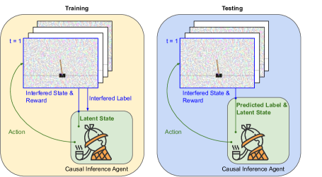
Figure 1: The proposed causal inference Q-network (CIQ) training and test framework, where the latent state is an unobserved (hidden) confounder variable. We refer the readers to Figure 3 for detailed descriptions on its graphical model.

In this paper, we evaluate the performance of our method in four environments: 1) Cartpole-v0 – the continuous control environment (Brockman et al. 2016); 2) the 3D graphical Banana Collector (Juliani et al. 2018)); 3) an Atari environment LunarLander-v2 (Brockman et al. 2016), and 4) pixel Cartpole – visual learning from the pixel inputs of Cartpole. For each of the environments, we consider four types of interference: (a) black-out, (b) Gaussian noise, (c) frozen screen, and (d) additive noise from adversarial perturbation.

In the testing phase mimicking the practical scenario that the agent may have interfered observations but is unaware of the true interference labels (i.e., happens or not), the results show that our CIQ method can perform better and more resilience against all the four types of interference. Furthermore, to benchmark the level of resilience of different RL models, we propose a new robustness measure, called CLEVER-Q, to evaluate the robustness of Q-network based RL algorithms. The idea is to compute a lower bound on the observation noise level such that the greedy action from the Q-network will remain the same against any noise below the lower bound. According to this robustness analysis, our CIQ algorithm indeed achieves higher CLEVER-Q scores compared with the baseline methods.

The main contributions of this paper include 1) a framework to evaluate the resilience of DQN-based DRL methods under abrupt observational interferences; 2) the proposed CIQ architecture and algorithm towards training a resilient DQN agent, and 3) an extreme-value theory based robustness metric (CLEVER-Q) for quantifying the resilience of Q-network based RL algorithms.

Related Works

Causal Inference for Generative Reinforcement Learning: Causal inference (Greenland, Pearl, and Robins 1999; Pearl 2009; Pearl, Glymour, and Jewell 2016; Pearl 2019; Robins, Rotnitzky, and Zhao 1995) has been used to empower the learning process under noisy observation and have better interpretability on deep learning models (Shalit, Johansson, and Sontag 2017; Louizos et al. 2017), also with efforts (Jaber, Zhang, and Bareinboim 2019; Forney, Pearl, and Bareinboim 2017; Bareinboim, Forney, and Pearl 2015; Bennett et al. 2021; Jung, Tian, and Bareinboim 2021) on causal online learning and bandit methods. Defining causation and applying causal inference framework to DRL still remains relatively unexplored. Recent works (Lu, Schölkopf, and Hernández-Lobato 2018; Tennenholtz, Mannor, and Shalit 2019) study this problem by defining action as one kind of intervention and estimating the causal effects. In contrast, we introduce observational interference into generative DRL by applying extra noisy and uncertain inventions. Inspired by the treatment switching and representation learning models (Shalit, Johansson, and Sontag 2017; Louizos et al. 2017; Helwegen, Louizos, and Forré 2020), we leverage the causal effect of observational interferences on states, and design an end-to-end structure for learning a causal-observational representation evaluating treatment effects on rewards.

Adversarial Perturbation: An intensifying challenge against deep neural network based systems is adversarial perturbation for making incorrect decisions. Many gradient-based noise-generating methods (Goodfellow, Shlens, and Szegedy 2015; Huang et al. 2017; Everett 2021) have been conducted for misclassification and mislead an agent’s output action. As an example of using DRL model playing Atari games, an adversarial attacker (Lin et al. 2017; Yang et al. 2020b) could jam in a timely and barely detectable noise to maximize the prediction loss of a Q-network and cause massively degraded performance.

Partially Observable Markov Decision Processes (POMDPs): Our resilient RL framework can be viewed as a POMDP with interfered observations. Belief-state methods are available for simple POMDP problems (e.g., plan graph and the tiger problem (Kaelbling, Littman, and Cassandra 1998)), but no provably efficient algorithm is available for general POMDP settings (Papadimitriou and Tsitsiklis 1987; Gregor et al. 2018). Recently, Igl et. al (Igl et al. 2018) have proposed a DRL approach for POMDPs by combining variational autoencoder and policy-based learning, but this kind of methods do not consider the interference labels available during training in our resilient RL framework.

Resilient Reinforcement Learning

In this section, we formally introduce our resilient RL framework and provide an extreme-value theory based metric called CLEVER-Q for measuring the robustness of DQN-based methods.

We consider a sequential decision-making problem where an agent interacts with an environment. At each time $t$, the agent gets an observation $x_{t}$, e.g. a frame in a video environment. As in many RL domains (e.g., Atari games), we view $s_{t}=(x_{t-M+1},\ldots,x_{t})$ to be the state of the environment where $M$ is a fixed number for the history of observations. Given a stochastic policy $\pi$, the agent chooses an action $a_{t}\sim\pi(s_{t})$ from a discrete action space based on the observed state and receives a reward $r_{t}$ from the environment. For a policy $\pi$, define the Q-function $Q^{\pi}(s,a)=\mathbb{E}\big{[}\sum_{t=0}^{\infty}\gamma^{t}r_{t}|s_{0}=s,\,a_{0}=a,\pi\big{]}$ where $\gamma\in(0,1)$ is the discount factor. The agent’s goal is to find the optimal policy $\pi^{*}$ that achieves the optimal Q-function given by $Q^{*}(s,a)=\max_{\pi}Q^{\pi}(s,a)$.

Resilience base on an Interventional Perspective

To evaluate the resilience ability of RL agents, we introduce additional interference as auxiliary information (as illustrated in Fig 1 ) as an empirical process  (Pearl 2009; Louizos et al. 2017) for observation. Given a type of interference $\mathcal{I}$, the agent’s observation becomes:

$$x^{\prime}_{t}=F^{\mathcal{I}}(x_{t},i_{t})=i_{t}\times\mathcal{I}(x_{t})+(1-i_{t})\times x_{t}$$ (1)

where $i_{t}\in\{0,1\}$ is the label indicating whether the observation is interfered at time $t$ or not, and $\mathcal{I}(x_{t})$ is the interfered observation.

We assume that interference labels $i_{t}$ follow an i.i.d. Bernoulli process with a fixed interference probability $p^{\mathcal{I}}$ as a noise level. For example, when $p^{\mathcal{I}}$ equals to 10%, each observational state has a 10% chance to be intervened under a perturbation. In this work, we consider the original observations, as illustrated in Figure 2 (a), under four types of interference as described below.

Gaussian Noise. Gaussian noise or white noise is a common interference to sensory data (Osband et al. 2019; Yurtsever et al. 2020). The interfered observation becomes $\mathcal{I}(x_{t})=x_{t}+n_{t}$ with a zero-mean Gaussian noise $n_{t}$. The noise variance is set to be the variance of all recorded states as illustrated in Figure 2 (b).

Adversarial Observation. Following the standard adversarial RL attack setting, we use fast gradient sign method (FGSM) (Szegedy et al. 2014) to generate adversarial patterns against the DQN loss (Huang et al. 2017) as illustrated in Figure 2 (c). The observation is given by $\mathcal{I}(x_{t})=x_{t}+\epsilon\operatorname{sign}\left(\nabla_{x_{t}}Q(x_{t},y;\theta)\right)$ where $y$ is the optimal action by weighting over possible actions.

Observation Black-Out. Off-the-shelf hardware can affect the entire sensor networks as a sensing background (Yurtsever et al. 2020) over-shoot with $\mathcal{I}(x_{t})=0$ (Yan, Xu, and Liu 2016). This perturbation is realistic owing to overheat hardware and losing the observational information of sensors.

Frozen Frame. Lagging and frozen frame(s) (Kalashnikov et al. 2018) often come from limited data communication bottleneck bandwidth. A frozen frame is given by $\mathcal{I}(x_{t})=x_{t-1}$. If the perturbation is constantly present, the frame will remain the first frozen frame since the perturbation happened.

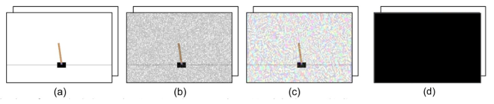
Figure 2: Visualization of perturbed observation (state) under uncertainty: (a) original state; (b) Gaussian perturbation; (c) adversarial perturbation (Huang et al. 2017), and (d) black-out perturbation (a white-out ablation in the Appendix E).

Resilient Reinforcement Learning Framework

With observational interference, instead of the actual state $s_{t}$, the agent only observes $s^{\prime}_{t}=(x^{\prime}_{t-M+1},\ldots,x^{\prime}_{t})$. The agent now needs to choose its actions $a_{t}\sim\pi(s^{\prime}_{t})$ based on the interfered observation. The resilient RL objective for the agent is to find a policy $\pi$ to maximize rewards in this environment under observational interference. Under the resilient framework, the goal of a Q-learning based agent is to learn the relation between $s^{\prime}_{t}$ and $Q_{t}$ where $Q_{t}(a)=\max_{\pi}\mathbb{E}\big{[}\sum_{\tau=t}^{\infty}\gamma^{(\tau-t)}r_{\tau}|s^{\prime}_{t},\,a_{t}=a,\pi\big{]}$ denotes the Q-values given the interfered observation $s^{\prime}_{t}$ at time $t$.

From the RL model and the observation model of Eq. (1), the relation among the observation $s^{\prime}_{t}$, Q-values $Q_{t}$, and interference $i_{t}$ can be described by a causal graphical model (CGM) in Figure 3. In the CGM, $z_{t}=(s_{t},i_{t-M+1},\ldots,i_{t})$ includes the actual state $s_{t}$ of the system together with the interference labels which causally affects all $s^{\prime}_{t}$, $Q_{t}$, and $i_{t}$. Note that $z_{t}$ is not observable to the agent due to the interference; $z_{t}$ could be viewed as a hidden confounder in causal inference.

Since only the interfered observation $s^{\prime}_{t}$ is available, the interference label $i_{t}$ is also non-observable in evaluating the resilience ability of an agent. However, the interference information is often accessible in the training phase, such as the use of a navigation simulator recorded with noisy augmentation (Grigorescu et al. 2020) for simulating interference in the training environment. We will discuss in the next subsection the benefit of utilizing the interference labels to improve learning efficiency.

Learning with Interference Labels

The goal of a resilient RL agent is to learn $P(Q_{t}|s^{\prime}_{t})$ to infer the Q-value $Q_{t}$ based on the interfered observation $s^{\prime}_{t}$. Note that one can compute $P(Q_{t}|s^{\prime}_{t})$ by determining the joint distribution $P(z_{t},s^{\prime}_{t},i_{t},Q_{t})$ of all variables in the CGM in Figure 3. Despite the presence of the hidden variable $z_{t}$, similar to causal inference with hidden confounders (Louizos et al. 2017), estimating the joint distribution $P(z_{t},s^{\prime}_{t},i_{t},Q_{t})$ could be done efficiently when the agent is provided the interference labels $i_{t}$ during training. On the other hand, if only the observation $s^{\prime}_{t}$ is available, the agent can only directly estimate $P(Q_{t}|s^{\prime}_{t})$, which is less efficient in terms of training sample usage.

We provide the interference type $\mathcal{I}$ and the interference labels $i_{t}$ to efficiently train a resilient RL agent as shown in Figure 3(b); however, in the actual testing environment, the agent only has access to the interfered observations $x^{\prime}_{t}$ as in Figure 3(a).

(a) Training

(b) Testing

Figure 3: Causal graphical model (CGM) for the training phase (a) and the testing phase (b). White nodes $s^{\prime}_{t}$ and $Q_{t}$ are observable. Node $z_{t}=(s_{t},i_{t-M+1},\ldots,i_{t})$, colored by white, is not observable. Node $i_{t}$, colored by white in (b), is only observable during training.

Causal Inference Q-Network

With the observable variables $(s^{\prime}_{t},i_{t},Q_{t})$ in Figure 3(a) during training, we aim to learn a model to infer the Q-values by estimating the joint distribution $P(z_{t},s^{\prime}_{t},i_{t},Q_{t})$. Despite the underlying dynamics in the RL system, when we view the interference as a treatment, the CGM in Figure 3(a) resembles some common causal inference models with binary treatment information and hidden confounders (Louizos et al. 2017). In this kind of causal inference problems, by leveraging on the binary property for treatment information, TARNet (Shalit, Johansson, and Sontag 2017) and CEVAE (Louizos et al. 2017) introduced a binary switching neural architecture to efficiently learn latent models for causal inference.

Inspired by the switching mechanism for causal inference, we propose the causal inference Q-network, referred as CIQ, that maps the interfered observation $s^{\prime}_{t}$ into a latent state $z_{t}$, makes proper inferences about the interference condition $i_{t}$, and adjusts its policy based on the estimated interference.

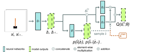
Figure 4: CIQ architecture. The notation $i^{train}_{t}$ denotes the inference label available during training, whereas $\tilde{i}_{t}$ is sampled during inference as $i_{t}$ is unknown.

We approximate the latent state by a neural network $\tilde{z}_{t}=f_{1}(x^{\prime}_{t};\theta_{1})$. From the latent state, we generate the estimated interference label $\tilde{i}_{t}\sim p(\tilde{i}_{t}|z_{t})=f_{I}(z_{t};\phi)$. We denote $s^{CI}_{t}=(\tilde{z}_{t-M+1},\tilde{i}_{t-M+1},\ldots,\tilde{z}_{t},\tilde{i}_{t})$ to be the causal inference state. As discussed in the previous subsection, the causal inference state acts as a confounder between the interference and the reward. Therefore, instead of using the interfered state $s^{\prime}_{t}$, the causal inference state $s^{CI}_{t}$ contains more relevant information for the agent to maximize rewards. Using the causal inference state helps focus on meaningful and informative details even under interference.

With the causal inference state $s^{CI}_{t}$, the output of the Q-network $Q(s^{CI}_{t};\theta)$ is set to be switched between two neural networks $f_{2}(s^{CI}_{t};\theta_{2})$ and $f_{3}(s^{CI}_{t};\theta_{3})$ by the interference label. Such a switching mechanism prevents our network from over-generalizing the causal inference state. During training, switching between the two neural networks is determined by the training interference label $i_{t}^{\text{train}}$. We assume that the true interference label is available in the training phase so $i_{t}^{\text{train}}=i_{t}$. In the testing, when $i_{t}$ is not available, we use the predicted interference label $\tilde{i}_{t}$ as the switch to decide which of the two neural networks to use.

All the neural networks $f_{1},f_{2},f_{3},f_{I}$ have two fully connected layers with each layer followed by the ReLU activation except for the last layer in $f_{2},f_{3}$ and $f_{I}$. The overall CIQ model is shown in Figure 4 and $\theta=(\theta_{1},\theta_{2},\theta_{3},\phi)$ denotes all its parameters. Note that, as common practice for discrete action spaces, the Q-network output $Q(s^{CI}_{t};\theta)$ is an $\mathcal{A}$-dimensional vector where $\mathcal{A}$ is the size of the action space, and each dimension represents the value for taking the corresponding action.

Finally, we train the CIQ model $Q(s^{\prime}_{t};\theta)$ end-to-end by the DQN algorithm with an additional loss for predicting the interference label. The overall CIQ objective function is defined as:

$$L^{\text{CIQ}}(\theta_{1},\theta_{2},\theta_{3},\phi)=i_{t}^{\text{train}}\cdot L^{\text{DQN}}(\theta_{1},\theta_{2},\phi)$$

$$+(1-i_{t}^{\text{train}})\cdot L^{\text{DQN}}(\theta_{1},\theta_{3},\phi)+\lambda\cdot(i_{t}^{\text{train}}\log p(\tilde{i}_{t}|\tilde{z}_{t};\theta_{1},\phi)$$

$$+(1-i_{t}^{\text{train}})\log(1-p(\tilde{i}_{t}|\tilde{z}_{t};\theta_{1},\phi))),$$ (2)

where $\lambda$ is a scaling constant and is set to 1 for simplicity. Due to the design of the causal inference state and the switching mechanism, we will show that CIQ can perform resilient behaviors against the observation interferences. We introduce how to quantify the robustness of a Q-network under noisy observation in next subsection. The CIQ training procedure (Algorithm 1) and an advanced CIQ based on variational inference (Louizos et al. 2017) are described in Appendix B.

CLEVER-Q: A Robustness Evaluation Metric for Q-Networks

Here we provide a comprehensive score (CLEVER-Q) for evaluating the robustness of a Q-network model by extending the CLEVER robustness score  (Weng et al. 2018) designed for classification tasks to Q-network based DRL tasks. Consider an $\ell_{p}$-norm bounded ($p\geq 1$) perturbation $\delta$ to the state $s_{t}$. We first derive a lower bound $\beta_{L}$ on the minimal perturbation to $s_{t}$ for altering the action with the top Q-value, i.e., the greedy action. For a given $s_{t}$ and a Q-network, this lower bound $\beta_{L}$ provides a robustness guarantee that the greedy action at $s_{t}$ will be the same as that of any perturbed state $s_{t}+\delta$, as long as the perturbation level $\|\delta\|_{p}\leq\beta_{L}$. Therefore, the larger the value $\beta_{L}$ is, the more resilience of the Q-network against perturbations can be guaranteed. Our CLEVER-Q score uses the extreme value theory to evaluate the lower bound $\beta_{L}$ as a robustness metric for benchmarking different Q-network models. The proof of Theorem 1. is available in Appendix B.

Theorem 1.

Consider a Q-network $Q(s,a)$ and a state $s_{t}$. Let $\mathcal{A}^{*}=\operatorname*{arg\,max}_{a}Q(s_{t},a)$ be the set of greedy (best) actions having the highest Q-value at $s_{t}$ according to the Q-network. Define $g_{a}(s_{t})=Q(s_{t},\mathcal{A}^{*})-Q(s_{t},a)$ for every action $a$, where $Q(s_{t},\mathcal{A}^{*})$ denotes the best Q-value at $s_{t}$. Assume $g_{a}(s_{t})$ is locally Lipschitz continuous with its local Lipschitz constant denoted by $L_{q}^{a}$, where $1/p+1/q=1$ and $p\geq 1$. For any $p\geq 1$, define the lower bound

$$\beta_{L}=min_{a\notin\mathcal{A}^{*}}g_{a}(s_{t})/L_{q}^{a}.$$ (3)

Then for any $\delta$ such that $\|\delta\|_{p}\leq\beta_{L}$, we have $\operatorname*{arg\,max}_{a}Q(s_{t},a)=\operatorname*{arg\,max}_{a}Q(s_{t}+\delta,a)$.

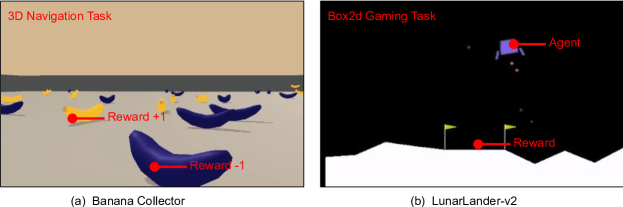
Figure 5: Illustration of our environments on: (a) a 3D navigation task, banana collector (Juliani et al. 2018), and (b) a video game, LunarLander (Brockman et al. 2016).

Experiments

Environments for DQNs

Our testing platforms were based on (a) OpenAI Gym (Brockman et al. 2016), (b) Unity-3D environments (Juliani et al. 2018), (c) a 2D gaming environment (Brockman et al. 2016), and (d) visual learning from pixel inputs of cart pole. Our test environments cover some major application scenarios and feature discrete actions for training DQN agents with the CLEVER-Q analysis. For instance, Atari games and space-invaders are popular real-world applications. Unity 3D banana navigation is a physical simulator but provides virtual to real options for further implementations.

Vector Cartpole: Cartpole (Sutton et al. 1998) is a classical continuous control problem. We use Cartpole-v0 from Gym (Brockman et al. 2016) with a targeted reward $=195.0$. The defined environment is manipulated by adding a force of $+1$ or $-1$ to a moving cart.

Banana Collector: The Banana collector shown in Figure 5 (a) is one of the Unity 3D baseline (Juliani et al. 2018). Different from the MuJoCo simulators with continuous actions, the Banana collector is controlled by four discrete actions corresponding to moving directions. The targeted reward is $12.0$ points by accessing correct bananas ($+1$). The state-space has 37 dimensions included velocity and a ray-based perception of objects around the agent.

Lunar Lander: Similar to the Atari gaming environments, Lunar Lander-v2 (Figure 5 (c)) is a discrete action environment from OpenAI Gym (Brockman et al. 2016) to control firing ejector with a targeted reward of $200$. The state is an eight-dimensional vector that records the lander’s position, velocity, angle, and angular velocities. The episode finishes if the lander crashes or comes to rest, receiving a reward $-100$ or $+100$ Firing ejector costs $-0.3$ each frame with $+10$ for each ground contact.

Pixel Cartpole: To further evaluate our models, we conduct experiments from the pixel inputs in the cartpole environment as a visual learning task. The size of input state is $400\times 600$. We use a max-pooling and a convolution layer to extract states as network inputs. The environment includes two discrete actions $\left\{left,right\right\}$, which is identical to the Cartpole-v0 of the vector version.

Baseline Methods

In the experiments, we compare our CIQ algorithm with two sets of DQN-based DRL baselines to demonstrate the resilience capability of the proposed method. We ensure all the models have the same number of 9.7 millions parameters with careful fine-tuning to avoid model capacity issues.

Pure DQN: We use DQN as a baseline in our experiments. The DQN agent is trained and tested on interfered state $s^{\prime}_{t}$. We also evaluate common DQN improvements in Appendix C and find the improvements (e.g., DDQN) have no significant effect against interference.

DQN with an interference classifier (DQN-CF): In the resilient reinforcement learning framework, the agent is given the true interference label $i_{t}^{\text{train}}$ at training. Therefore, we would like to provide this additional information to the DQN agent for a fair comparison. During training, the interfered state $s^{\prime}_{t}$ is concatenated with the true label $i_{t}^{\text{train}}$ as the input for the DQN agent. Since the true label is not available at testing, we train an additional binary classifier (CF) for the DQN agent. The classifier is trained to predict the interference label, and this predicted label will be concatenated with the interfered state as the input for the DQN agent during testing.

DQN with safe actions (DQN-SA): Inspired by shielding-based safe RL (Alshiekh et al. 2018), we consider a DQN baseline with safe actions (SA). The DQN-SA agent will apply the DQN action if there is no interference. However, if the current observation is interfered, it will choose the action used for the last uninterfered observation as the safe action. This action-holding method is also a typical control approach when there are missing observations (Franklin et al. 1998). Similar to DQN-CF, a binary classifier for interference is trained to provide predicted labels at testing.

DVRLQ and DVRLQ-CF: Motivated by deep variational RL (DVRL) (Igl et al. 2018), we provide a version of DVRL as a POMDP baseline. We call this baseline DVRLQ because we replace the A2C-loss with the DQN loss. Similar to DQN-CF, we also consider another baseline of DVRLQ with a classifier, referred to as DVRLQ-CF, for a fair comparison using the interference labels.

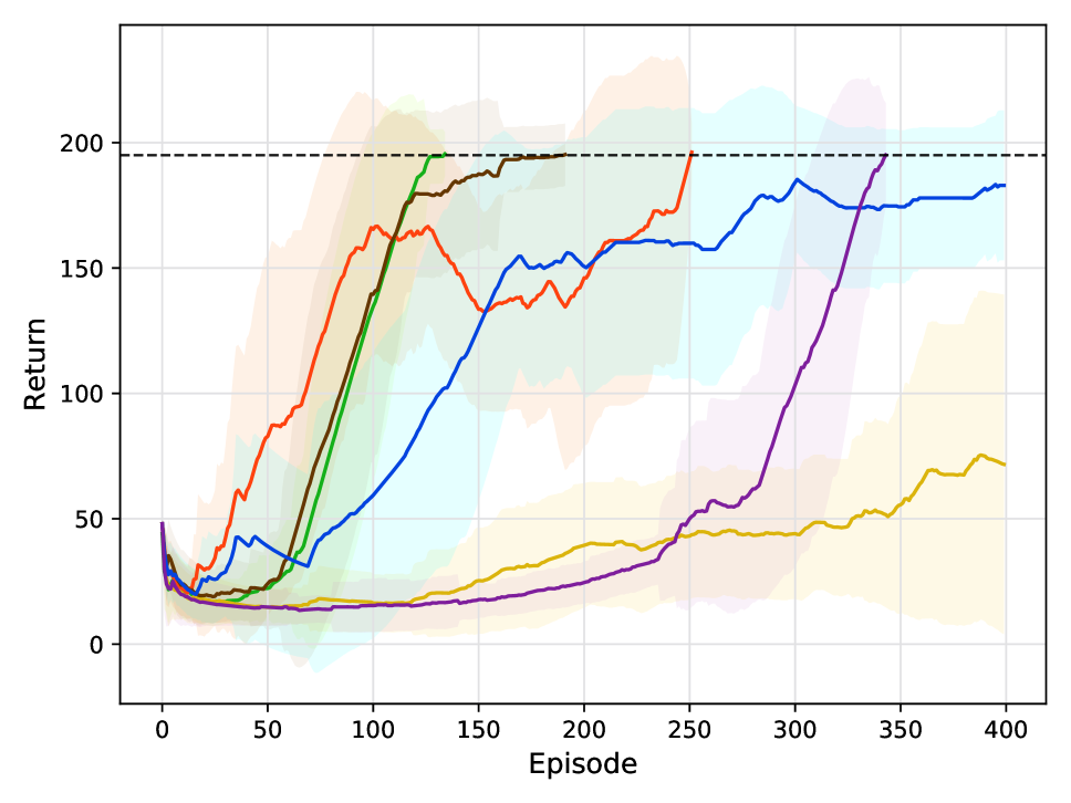
(a) Cartpole${}^{adversarial}_{vector}$.

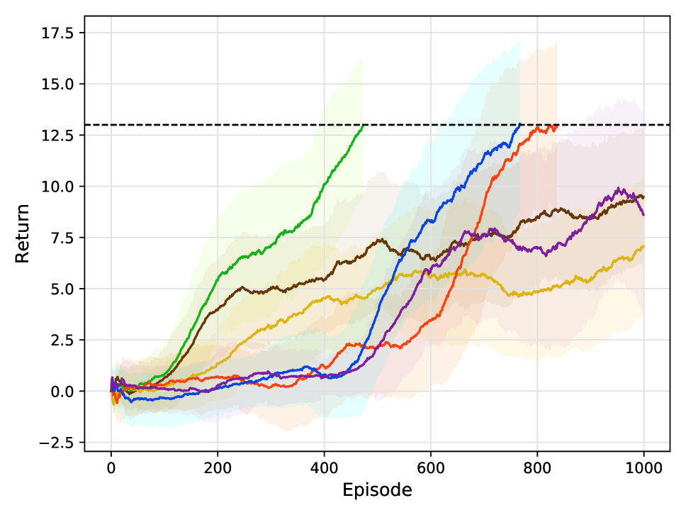
(b) Banana^adversarial.

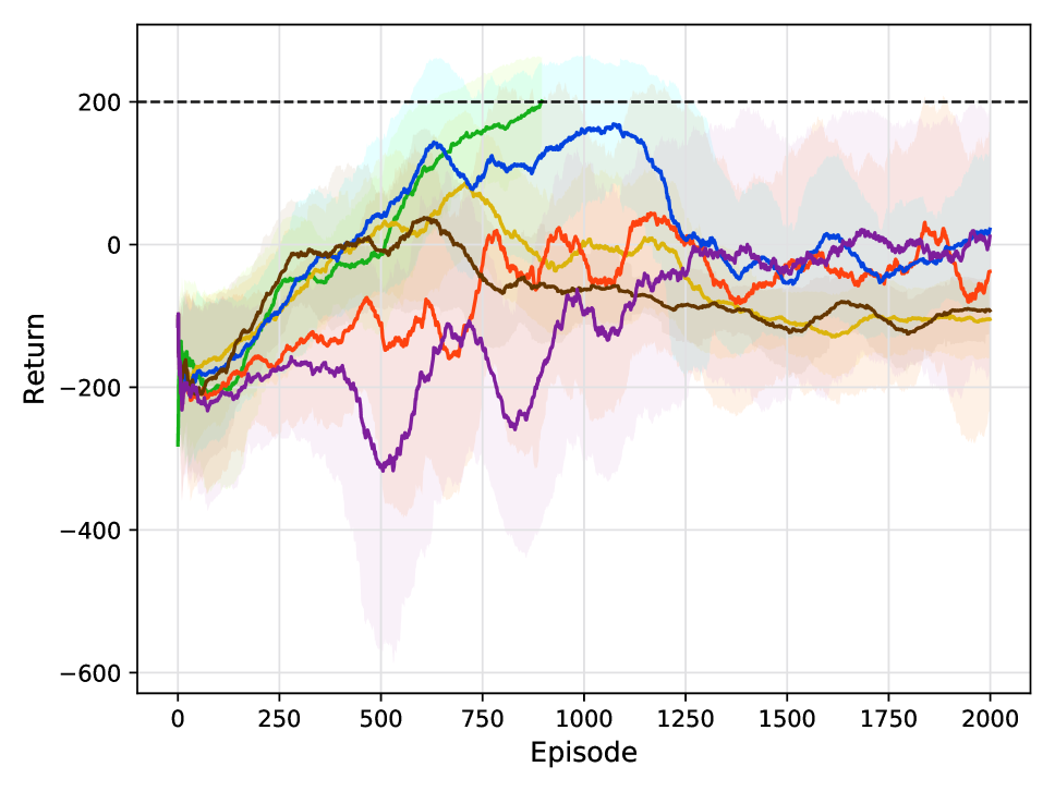
(c) Lunar^adversarial.

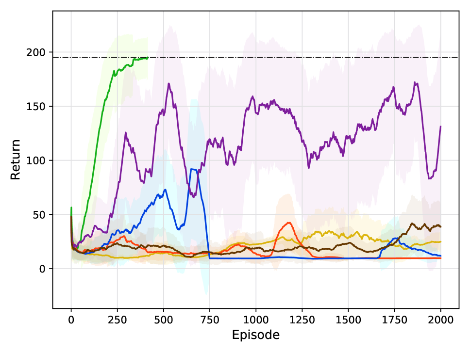
(d) Cartpole${}^{adversarial}_{pixel}$.

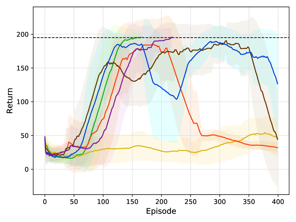
(e) Cartpole${}^{blackout}_{vector}$.

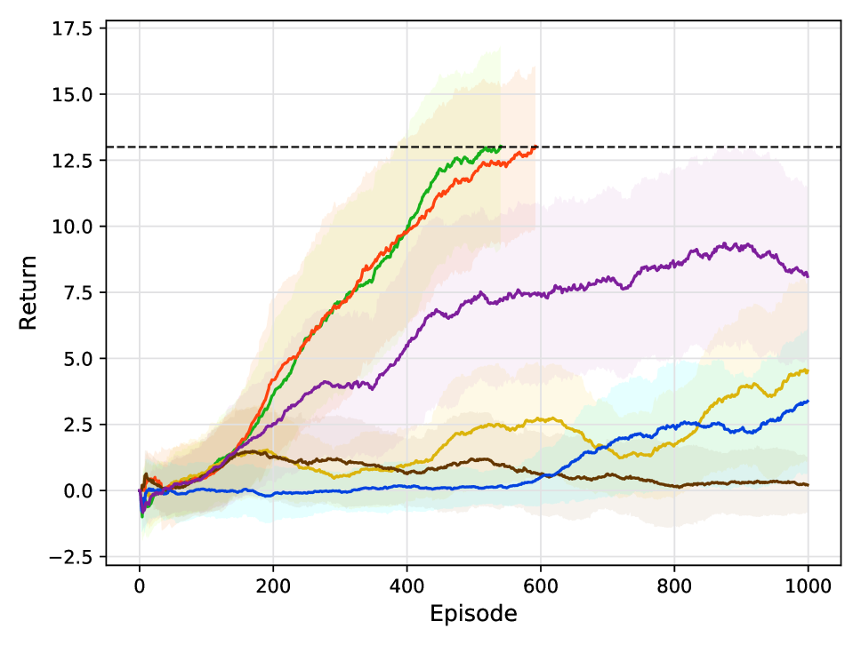
(f) Banana^blackout.

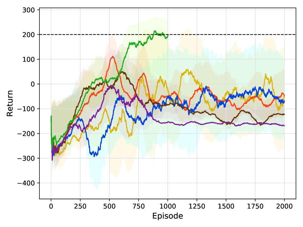
(g) Lunar^blackout

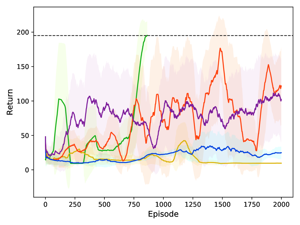
(h) Cartpole${}^{blackout}_{pixel}$.

Figure 6: Performance of DQNs under potential (20%) adversarial and black-out interference.

Table 1: Performance resilience analysis of AC-Rate ($\uparrow$) and CLEVER-Q robustness score ($\uparrow$) under additive Gaussian ($l_{2}$-norm) and adversarial ($l_{\infty}$-norm) perturbations on state in the vector Cartpole environment.

$\mathcal{I}$=L2	AC-Rate		CLEVER-Q		$\mathcal{I}$=L∞	AC-Rate		CLEVER-Q
P%, $\mathcal{I}$	DQN	CIQ	DQN	CIQ	P%, $\mathcal{I}$	DQN	CIQ	DQN	CIQ
10%	82.10%	99.61%	0.176	0.221	10%	62.23%	99.52%	0.169	0.248
20%	72.15%	98.52%	0.130	0.235	20%	9.68%	98.52%	0.171	0.236
30%	69.74%	98.12%	0.109	0.232	30%	1.22%	98.10%	0.052	0.230

Resilient RL on Average Returns

We run performance evaluation with six different interference probabilities ($p^{I}$ in Sec. Resilience base on an Interventional Perspective), including $\left\{0\%,10\%,20\%,30\%,40\%,50\%\right\}$. We train each agent $50$ times and highlight its standard deviation with lighter colors. Each agent is trained until the target score (shown as the dashed black line) is reached or until 400 episodes. We show the average returns for $p^{I}=20\%$ under adversarial perturbation and black-out in Figure 6 and report the rest of the results in Appendix B.

CIQ (green) clearly outperforms all the baselines under all types of interference, validating the effectiveness of our CIQ in learning to infer and gaining resilience against a wide range of observational interferences. Pure DQN (yellow) cannot handle the interference with $20\%$ noise level. DQN-CF (orange) and DQN-SA (brown) have competitive performance in some environments against certain interferences, but perform poorly in others. DVRLQ (blue) and DVRLQ-CF (purple) cannot achieve the target reward in most experiments and this might suggest the inefficiency of applying a general POMDP approach in a framework with a specific structure of observational interference.

Robustness Metrics based on Recording States

We evaluate the robustness of DQN and CIQ by the proposed CLEVER-Q metric. To make the test state environment consistent among different types and levels of interference, we record the interfered states, $S_{N}=\mathcal{I}(S_{C})$, together with their clean states, $S_{C}$. We then calculate the average CLEVER-Q for DQN and CIQ based on the clean states $S_{C}$ using Eq. 3 over 50 times experiments for each agent.

We also consider a retrospective robustness metric, the action correction rate (AC-Rate). Motivated by previous off-policy and error correction studies (Dulac-Arnold et al. 2012; Harutyunyan et al. 2016; Lin et al. 2017), AC-Rate is defined as the action matching rate $R_{Act}=\frac{1}{T}\sum_{t=0}^{T-1}\mathbf{1}_{\{a_{t}=a^{*}_{t}\}}$ between $a_{t}$ and $a^{*}_{t}$ over an episode with length $T$. Here $a_{t}$ denotes the action taken by the agent with interfered observations $S_{N}$, and $a^{*}_{t}$ is the action of the agent if clean states $S_{C}$ were observed instead.

The roles of CLEVER-Q and AC-Rate are complementary as robustness metrics. CLEVER-Q measures sensitivity in terms of the margin (minimum perturbation) required for a given state to change the original action. AC-rate measures the utility in terms of action consistency. Altogether, they provide a comprehensive resilience assessment.

Table 1 reports the two robustness metrics for DQN and CIQ under two types of interference. CIQ attains higher scores than DQN in both CLEVER-Q and AC-Rate, reflecting better resilience in CIQ evaluations. We provide more robustness measurements in Appendix A and D.

Average Treatment Effect under Intervention

In a causal learning setting, evaluating treatment effects and conducting statistical refuting experiments are essential to support the underlying causal graphical model. Through resilient reinforcement learning framework, we could interpret DQN by estimating the average treatment effect (ATE) of each noisy and adversarial observation. We first define how to calculate a treatment effect in the resilient RL settings and conduct statistical refuting tests including random common cause variable test ($T_{c}$), replacing treatment with a random (placebo) variable ($T_{p}$), and removing a random subset of data ($T_{s}$). The open-source causal inference package Dowhy (Sharma, Kiciman et al. 2019) is used for analysis.

We refine a Q-network with discrete actions for estimating treatment effects based on Theorem 1 in (Louizos et al. 2017). In particular, individual treatment effect (ITE) can be defined as the difference between the two potential outcomes of a Q-network; and the average treatment effect (ATE) is the expected value of the potential outcomes over the subjects. In a binary treatment setting, for a Q-value function $Q_{t}(s_{t})$ and the interfered state $\mathcal{I}(s_{t})$, the ITE and ATE are calculated by:

$$Q_{t}^{ITE}=Q_{t}(s_{t})\left(1-p_{t}\right)+Q_{t}({\mathcal{I}}(s_{t}))p_{t}$$ (4)

$$ATE=\sum_{t=1}^{\mathcal{T}}\frac{\mathbb{E}\left[Q_{t}^{ITE}({\mathcal{I}}(s_{t}))\right]-\mathbb{E}\left[Q_{t}^{ITE}(s_{t})\right]}{\mathcal{T}}$$ (5)

where $p_{t}$ is the estimated inference label by the agent and $\mathcal{T}$ is the total time steps of each episode. As expected, we find that CIQ indeed attains a better ATE and its significance can be informed by the refuting tests based on $T_{c}$, $T_{p}$ and $T_{s}$. We refer to Appendix C for more details.

Additional analysis

We also conduct the following analysis to better understand our CIQ model. Environments with a dynamic noise level are evaluated. Due to the space limit, see their details in appendix B to D. Furthermore, a discussion on the advantage of sample complexity benefited from sequential learning with interference labels is included in Appendix B.

Neural saliency map: We apply the perturbation-based saliency map for DRL (Greydanus et al. 2018) as shown in Figure 7 and appendix Dto visualize the saliency centers of CIQ and others, which is based on the Q-value of each model as interpretable studies.

Treatment effect analysis: We provide treatment effect analysis on each kind of interference to statistically verify the CGM with lowest errors on average treatment effect refutation in appendix C.

Ablation studies: We conduct ablation studies by comparing several CIQ variants, each without a certain CIQ component, and verify the importance of the proposed CIQ architecture in Appendix D for future studies.

Test on different noise levels: We train CIQ under one noise level and test on another level, which shows that the difference in noise level does not affect much on the performance of CIQ model reported in Appendix B.

Transferability in robustness: Based on CIQ, we study how well can the robustness of different interference types transfer between training and testing environments. We evaluate two general settings (i) an identical interference type but different noise levels (Appendix D) and (ii) different interference types (Appendix D). Tab 3 summarizes the results.

Multiple interference types: We also provide a generalized version of CIQ that deals with multiple interference types in training and testing environments. Tab 2 summarizes the results. The generalized CIQ is equipped with a common encoder and individual interference decoders to study multi-module conditional inference, with some additional discussion in Appendix E.

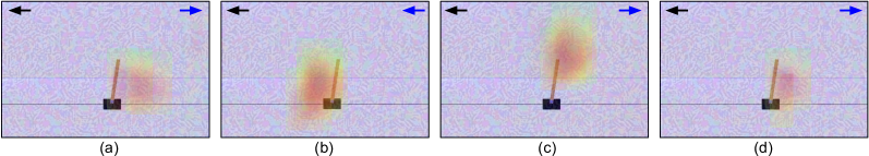
Figure 7: Perturbation-based saliency map on Pixel Cartpole under adversarial perturbation: (a) DQN, (b) CIQ, (c) DQN-CF; (d) DVRLQ-CF. The black arrows are correct actions and blue arrows are agents’ actions. The neural saliency of CIQ makes more correct actions responding to ground actions.

Table 2: Stability test of proposed CIQ (Train Noise-Level, Test Noise-Level). We consider settings with different training and testing noise levels for CIQ evaluation afterward.

Metrics (0.1, 0.3) (0.3, 0.1) (0.3, 0.2) (0.3, 0.3) (0.3, 0.4) (0.3, 0.5) Performance 182.8 195.0 195.0 195.0 195.0 185.7 CLEVER-Q 0.195 0.239 0.232 0.230 0.224 0.215 AC-Rate 0.914 0.985 0.986 0.995 0.984 0.924

Table 3: CIQ-MI: CIQ agent with an extended multi-interference (MI) architecture testing in Env₁ (noise level $P=20\%$). As a proof of concept, we consider two interference types together, Gaussian noise and adversarial perturbation. In this setting every observation (state) can possibly undergo an interference with either Gaussian noise or Adversarial perturbation. CIQ-MI is capable of making correct action to solve (over 195.0) the testing environment when training with mixed interference types.

Train / Test Gaussian Adversarial Gaussian + Adversarial Gaussian 195.1 154.2 96.3 Adversarial 153.9 195.0 105.1 Gaussian + Adversarial 195.0 195.0 195.0

Conclusion

Our experiments suggest that, although some DQN-based DRL algorithms can achieve high scores under the normal condition, their performance can be severely degraded in the presence of interference. In order to be resilient against interference, we propose CIQ, a novel causal-inference-driven DRL algorithm. Evaluated on a wide range of environments and multiple types of interferences, the CIQ results show consistently superior performance over several RL baseline methods. We investigate the improved resilience of CIQ by CLEVER-Q and AC-Rate metrics. Our demo code is available at github.com/huckiyang/Obs-Causal-Q-Network.

Appendix A Appendix

Our supplementary sections included:

• A. Proof of the CLEVER-Q Theorem and Additional Robustness Measurements

• B. Implementation Details and Additional Results

• C. Causal Relation Evaluation and Average Treatment Effects in CIQ Networks

• D. Ablation Studies

Appendix B A. Proof of the CLEVER-Q Theorem and Additional Robustness Measurements

Proof of the CLEVER-Q Theorem

Here we provide a comprehensive score (CLEVER-Q) for evaluating the robustness of a Q-network model by extending the CLEVER robustness score  (Weng et al. 2018) designed for classification tasks to Q-network based DRL tasks. Consider an $\ell_{p}$-norm bounded ($p\geq 1$) perturbation $\delta$ to the state $s_{t}$. We first derive a lower bound $\beta_{L}$ on the minimal perturbation to $s_{t}$ for altering the action with the top Q-value, i.e., the greedy action. For a given $s_{t}$ and a Q-network, this lower bound $\beta_{L}$ provides a robustness guarantee that the greedy action at $s_{t}$ will be the same as that of any perturbed state $s_{t}+\delta$, as long as the perturbation level $\|\delta\|_{p}\leq\beta_{L}$. Therefore, the larger the value $\beta_{L}$ is, the more resilience of the Q-network against perturbations can be guaranteed. Our CLEVER-Q score uses the extreme value theory to evaluate the lower bound $\beta_{L}$ as a robustness metric for benchmarking different Q-network models.

Theorem 2.

Consider a Q-network $Q(s,a)$ and a state $s_{t}$. Let $\mathcal{A}^{*}=\operatorname*{arg\,max}_{a}Q(s_{t},a)$ be the set of greedy (best) actions having the highest Q-value at $s_{t}$ according to the Q-network. Define $g_{a}(s_{t})=Q(s_{t},\mathcal{A}^{*})-Q(s_{t},a)$ for every action $a$, where $Q(s_{t},\mathcal{A}^{*})$ denotes the best Q-value at $s_{t}$. Assume $g_{a}(s_{t})$ is locally Lipschitz continuous with its local Lipschitz constant denoted by $L_{q}^{a}$, where $1/p+1/q=1$ and $p\geq 1$. Then for any $p\geq 1$, define the lower bound

$$\beta_{L}=min_{a\notin\mathcal{A}^{*}}g_{a}(s_{t})/L_{q}^{a}.$$

Then for any $\delta$ such that $\|\delta\|_{p}\leq\beta_{L}$,

$$\operatorname*{arg\,max}_{a}Q(s_{t},a)=\operatorname*{arg\,max}_{a}Q(s_{t}+\delta,a)$$

Proof.

Because $g_{a}(s_{t})$ is locally Lipschitz continuous, by Holder’s inequality, we have

$$|g_{a}(x)-g_{a}(y)|\leq L_{q}^{a}||x-y||_{p},$$ (6)

for any $x,y$ within the $R_{p}$-ball centered at $s_{t}$. Now let $x=s_{t}$ and $y=s_{t}+\delta$, where $\delta$ is some perturbation. Then

$$g_{a}(s_{t})-L_{q}^{a}||\delta||_{p}\leq g_{a}(s_{t}+\delta)\leq g_{a}(s_{t})+L_{q}^{a}.||\delta||_{p}$$ (7)

Note that if $g_{a}(s_{t}+\delta)\geq 0$, then $A^{*}$ still remains as the top Q-value action set at state $s_{t}+\delta$. Moreover, $g_{a}(s_{t})-L_{q}^{a}||\delta||_{p}\geq 0$ implies $g_{a}(s_{t}+\delta)\geq 0$. Therefore,

$$||\delta||_{p}\leq g_{a}(s_{t})/L_{q}^{a},$$ (8)

provides a robustness guarantee that ensures $Q(s_{t}+\delta,\mathcal{A}^{*})\geq Q(s_{t}+\delta,a)$ for any $\delta$ satisfying Eq. equation 6. Finally, to provide a robustness guarantee that $Q(s_{t}+\delta,\mathcal{A}^{*})\geq Q(s_{t}+\delta,a)$ for any action $a\notin\mathcal{A}^{*}$, it suffices to take the minimum value of the bound (for each $a$) in Eq. equation 6 over all actions other than $a^{*}$, which gives the lower bound

$$\beta_{L}=min_{a\notin A^{*}}g_{a}(s_{t})/L^{a}_{q}$$ (9)

∎

For computing $\beta_{L}$, while the numerator is easy to obtain, the local Lipschitz constant $L_{q}^{a}$ cannot be directly computed. In our implementation, by using the fact that $L_{q}^{a}$ is equivalent to the local maximum gradient norm (in $\ell_{q}$ norm), we use the same sampling technique from extreme value theory as proposed in (Weng et al. 2018) for estimating $L_{q}^{a}$.

Algorithm 1 CIQ Training

1:  Inputs: $Agent$, $NoisyEnv$, $Oracle$, $max\_step$, $NoisyEnv\_test$, $target$, $eval\_steps$

2:  Initialize: $t=0$, $score=0$, $s^{\prime}_{t}=NoisyEnv$.reset()

3:  while $t<max\_step$ and $score<target$ do

4:     $i_{t}$ = $oracle$($NoisyEnv$, $t$)

5:     $a_{t}$ = $Agent$.act($s_{t}^{\prime}$, $i_{t}$)

6:     $s_{t+1}^{\prime}$, $r_{t}$, $done$ = $NoisyEnv$.step($a_{t}$)

7:     $Agent$.learn($s_{t}^{\prime}$, $a_{t}$, $r_{t}$, $s_{t+1}^{\prime}$, $i_{t}$)

8:     if $t\in eval\_steps$ then

9:        $score$ = $Agent$.evaluate($NoisyEnv\_test$)

10:     end if

11:     if $done$ then

12:        $s_{t}^{\prime}$ = $NoisyEnv$.reset()

13:     else

14:        $s_{t}^{\prime}$ = $s_{t+1}^{\prime}$

15:     end if

16:     $t$ = $t$ + 1

17:  end while

18:  Return $Agent$

Background and Training Setting

To scale to high-dimensional problems, one can use a parameterized deep neural network $Q(s,a;\theta)$ to approximate the Q-function, and the network $Q(s,a;\theta)$ is referred to as the deep Q-network (DQN). The DQN algorithm (Mnih et al. 2015) updates parameter $\theta$ according to the loss function:

$$L^{\text{DQN}}(\theta)=\mathbb{E}_{(s_{t},a_{t},r_{t},s_{t+1})\sim D}\Big{[}(y^{\text{DQN}}_{t}-Q(s_{t},a_{t};\theta))^{2}\Big{]}$$

where the transitions $(s_{t},a_{t},r_{t},s_{t+1})$ are uniformly sampled from the replay buffer $D$ of previously observed transitions, and $y^{\text{DQN}}_{t}=r_{t}+\gamma\max_{a}Q(s_{t+1},a;\theta^{-})$ is the DQN target with $\theta^{-}$ being the target network parameter periodically updated by $\theta$.

Double DQN (DDQN) (Van Hasselt, Guez, and Silver 2016) further improves the performance by modifying the target to $y^{\text{DDQN}}_{t}=r_{t}+\gamma Q(s_{t+1},\operatorname*{arg\,max}_{a}Q(s_{t+1},a;\theta);\theta^{-}).$ Prioritized replay is another DQN improvement which samples transitions $(s_{t},a_{t},r_{t},s_{t+1})$ from the replay buffer according to the probabilities $p_{t}$ proportional to their temporal difference (TD) error: $p_{t}\propto|y^{\text{DDQN}}_{t}-Q(s_{t},a_{t};\theta)|^{\alpha}$ where $\alpha$ is a hyperparameter.

We use Pytorch 1.2 to design both DQN and causal inference Q (CIQ) networks in our experiments. Our code can be found in the supplementary material. We use Nvidia GeForce RTX 2080 Ti GPUs with CUDA 10.0 for our experiments. We use the Quantile Huber loss (Dabney et al. 2018) $\mathcal{L}_{\kappa}$ for DQN models with $\kappa=1$ in Sup-Eq. 11, which allows less dramatic changes from Huber loss:

$$\mathcal{L}_{\kappa}(u)=\left\{\begin{array}[]{ll}{\frac{1}{2}u^{2},}&{\text{ if }|u|\leq\kappa}\\ {\kappa\left(|u|-\frac{1}{2}\kappa\right),}&{\text{ otherwise }}\end{array}\right.$$ (10)

The quantile Huber loss (Dabney et al. 2018) is the asymmetric variant of the Huber loss for quantile $\tau\in[0,1]$ from Sup-Eq. 10:

$$\rho_{\tau}^{\kappa}(u)=\left|\tau-\delta_{\{u<0\}}\right|\mathcal{L}_{\kappa}(u).$$ (11)

After the a maximum update step in the temporal loss $u$ in Sup-Eq. 10, we synchronize $\theta_{i}^{-}$ with $\theta_{i}$ follow the implementation from the OpenAI baseline (Dhariwal et al. 2017) in Sup-Eq 12:

$$u_{i}\left(\theta_{i}\right)=\mathbb{E}\left(\underbrace{y^{\text{DDQN}}}_{\theta_{\text{target }}}-\underbrace{Q\left(s,a;\theta_{i}\right)}_{\theta_{\text{local }}}\right)^{2}.$$ (12)

We use the soft-update (Fox, Pakman, and Tishby 2015) to update the DQN target network as in Sup-Eq 13:

$$\theta_{\text{local}}=\tau\times\theta_{\text{local}}+(1-\tau)\times\theta_{\text{target}},$$ (13)

where $\theta_{\text{target}}$ and $\theta_{\text{local}}$ represent the two neural networks in DQN and $\tau$ is the soft update parameter depending on the task.

For each environment, in additional to the 5 baselines described in Section 4.2, we also evaluate the performance of common DQN improvements such as deep double Q-networks (DDQN) for DDQN with dueling (DDQN_d), DDQN with a prioritized replay (DDQN_p), DDQN with a joint-training interference classifier (DDQN-CF), and DDQN with a safe action reply (DDQN-SA). We test each model against four types of interference, Gaussian, Adversarial, Blackout, and Frozen Frame, with $p^{I}\in[10\%,20\%,30\%,40\%,50\%]$. We also consider a non-stationary noise-level sampling from a cosine-wave in a range of [0%, 30%] for every ten steps. CIQ shows a better and continuous performance to solve the environments before the noise level attaining 40% and under the cosine-noise. Compared to variational based DQNs methods, joint-trained DDQN-CF show a much obvious advantages when the noise levels are in the range of 40% to 50%.

Env₁: Cartpole Environment.

We use a four-layer neural network, which included an input layer, two 32-unit wide ReLU hidden layers, and an output layer (2 dimensions). The observation dimension of Cartpole-v1 (Brockman et al. 2016) is 4 and the input stacks 4 consecutive observations. The dimension of the input layer is [$4\times 4$]. We design a replay buffer with a memory of 100,000, with a mini-batch size of 32, the discount factor $\gamma$ is set to 0.99, the $\tau$ for a soft update of target parameter is $5\times 10^{-3}$, a learning rate for Adam (Kingma and Ba 2014) optimization is $5\times 10^{-4}$, a regularization term for weight decay is $1\times{10^{-4}}$, the coefficient $\alpha$ for importance sampling exponent is 0.6, the coefficient of prioritization exponent is 0.4.

Env₂: 3D Banana Collector Environment.

We utilize the Unity Machine Learning Agents Toolkit (Juliani et al. 2018), which is an open-source and reproducible 3D rendering environment for the task of Banana Collector. We use open-source graphic rendering version  with Unity backbone (Juliani et al. 2018) for reproducible DQN experiments, which is designed to render the collector agent for both Linux and Windows systems. A reward of $+1$ is provided for collecting a yellow banana, and a reward of $-1$ is provided for collecting a blue banana. We use a six-layer deep network, which includes an input layer, three 64-unit fully-connected ReLU hidden layers, and an output layer (2 dimensions). We use [$37\times 4$] for our input layer, which composes from the observation dimension (37) and the stacked input of 4 consecutive observations. We design a replay buffer with a memory of 100,000, with a mini-batch size of 32, the discount factor $\gamma$ is equal to 0.99, the $\tau$ for a soft update of target parameter is $10^{-3}$, a learning rate for Adam (Kingma and Ba 2014) optimization is $5\times 10^{-4}$, a regularization term for weight decay is $1\times{10^{-4}}$, the coefficient $\alpha$ for importance sampling exponent is 0.6, the coefficient of prioritization exponent is 0.4.

Env₃: Lunar Lander Environment.

The lunar lander-v2 (Brockman et al. 2016) is one of the most challenging environments with discrete actions. The observation dimension of Lunar Lander-v2 (Brockman et al. 2016) is 8 and the input stacks 10 consecutive observations. The objective of the game is to navigate the lunar lander spaceship to a targeted landing spot without a collision. A collection of six discrete actions controls two real-valued vectors ranging from -1 to +1. The first dimension controls the main engine on and off numerically, and the second dimension throttles from 50% to 100% power. The following two actions represent for firing left, and the last two actions represent for firing the right engine. The dimension of the input layer is [$8\times 10$]. We design a 7-layers neural network for this task, which includes 1 input layer, 2 layer of 32 unit wide fully-connected ReLU network, 2 layers deep 64-unit wide ReLU networks, (for all DQNs), 1 layer of 16 unit wide fully-connected ReLU network, and 1 output layer (4 dimensions). The replay buffer size is 500,000; the minimum batch size is 64, the discount factor is 0.99, the $\tau$ for a soft update of target parameters is $10^{-3}$, the learning rate is $5\times 10^{-4}$, the minimal step for reset memory buffer is 50. We train each model 1,000 times for each case and report the mean of the average final performance (average over all types of interference). Env₃ is a challenging task owing to often receive negative reward during the training. We thus consider a non-stationary noise-level sampling from a cosine-wave in a narrow range of [0%, 20%] for every ten steps. Results suggest CIQ could still solve the environment before the noise-level going over to 30%. For the various noisy test, CIQ attains a best performance over 200.0 the other DQNs algorithms (skipping the table since only CIQ and DQN-CF have solved the environment over 200.0 training with adversarial and blackout interference.)

Env₄: Pixel Cartpole Environment

To observe pixel inputs of Cartpole-v1 as states, we use a screen-wrapper with an original size of [400, 600, 3]. We first resize the original frame into a single gray-scale channel, [100, 150] from the RGN2GRAY function in the OpenCV. The implementation details are shown in the ”pixel_tool.py” and ”cartpole_pixel.py”, which could be refereed to the submitted supplementary code. Then we stack 4 consecutive gray-scale frames as the input. We design a 7-layer DQN model, which included input layer, the first hidden layer convolves 32 filters of a [$8\times 8$] kernel with stride 4, the second hidden layer convolves 64 filters of a [$4\times 4$] kernel with stride 2, the third layer is a fully-connected layer with 128 units, from fourth to fifth layers are fully-connected layer with 64 units, and the output layer (2 dimensions). The replay buffer size is 500,000; the minimum batch size is 32, the discount factor is 0.99, the $\tau$ for a soft update of target parameters is $10^{-3}$, the learning rate is $5\times 10^{-4}$, the minimal step for reset memory buffer is 1000.

Train and Test on Different Noise Level

We consider settings with different training and testing noise levels for CIQ evaluation. The (train, test)% case trains with train% noise then tests with test% noise. We observe that CIQ have the capability of learning transformable q-value estimation, which attain a succeed score of 195.00 in the noise level 30 $\pm$ 10%. Meanwhile, other DQNs methods included DDQN-CF, DVRLQ-CF, DDQN-SA perform a general performance decay in the test on different noise level. This result would be limited to the generalization of power and challenges (Bengio 2013; Higgins et al. 2018) in as disentangle unseen state of a single parameterized deep network.

Markovian Noise

We also provide a dynamic noise study for CIQ training with i.i.d. Gaussian interference, $p^{\mathcal{I}}=0.2$; testing with Markov distribution $P(i_{t}\!=\!1|i_{t-1}\!=\!1)\!=\!0.55$, $P(i_{t}\!=\!1|i_{t-1}\!=\!0)\!=\!0.05$, stationary $p^{\mathcal{I}}=0.1$ testing in Env₁ and Env₂. This experiment shows the learning power against unseen Markovian interference in Table 4, which further confirms CIQ’s ability against unseen interference distribution and dynamics.

Table 4: CIQ training against unseen interference distribution and dynamics

Model	DQN	CIQ	DQN-CF	DQN-SA	DVRLQ	DQN-VAE	DQN-CEVAE
Env1 Markov	112.3	195.0	181.4	131.4	112.1	163.7	155.6
Env2 Markov	9.4	12.1	11.7	9.1	11.5	11.2	11.2

Advantages of Training with Interference Labels

We provide an example to analytically demonstrate the learning advantage of having the interference labels during training. Consider an environment of i.i.d. Bernoulli states $s_{t}=x_{t}$ with $P(x_{t}=1)=P(x_{t}=0)=0.5$ and two actions $0$ and $1$. There is no reward taking action $a_{t}=0$. When $a_{t}=1$, the agent pays one unit to have a chance to win a two unit reward with probability $q_{x}$ at state $x_{t}=x\in\{0,1\}$. Therefore, $P(r_{t}=1|x_{t}=x,a_{t}=1)=q_{x}$ and $P(r_{t}=-1|x_{t}=x,a_{t}=1)=1-q_{x}$. This simple environment is a contextual bandit problem where the optimal policy is to pick $a_{t}=1$ at state $x_{t}=x$ if $q_{x}>0.5$, and $a_{t}=0$ if $q_{x}\leq 0.5$. If the goal is to find an approximately optimal policy, the agent should take action $a_{t}=1$ during training to learn the probabilities $q_{0}$ and $q_{1}$. Suppose the environment is subjected to observation black-out $x^{\prime}_{t}=0$ with $p^{\mathcal{I}}=0.2$ when $x_{t}=1$, and no interference when $x_{t}=0$. Assume $q_{0}=(3-q_{1})/5$. Then we have $P(r_{t}=1|x^{\prime}_{t}=1,a_{t}=1)=q_{1}$, and $P(r_{t}=1|x^{\prime}_{t}=0,a_{t}=1)=q_{0}P(x_{t}=0|x^{\prime}_{t}=0)+q_{1}P(x_{t}=1|x^{\prime}_{t}=0)=0.5$. If the agent only has the interfered observation $x^{\prime}_{t}$, the samples for $x^{\prime}_{t}=0$ are irrelevant to learning $q_{1}$ because rewards just randomly occur with probability half given $x^{\prime}_{t}=0$. Therefore, the sample complexity bound is proportional to $1/P(x^{\prime}_{t}=1)$ because only samples with $x^{\prime}_{t}=1$ are relevant. On the other hand, if the agent has access to the labels $i_{t}$ during training, even when observed $x^{\prime}_{t}=0$, the agent can infer whether $x_{t}=1$ by checking $i_{t}=1$ or not. Therefore, the causal relation allows the agent to learn $q_{1}$ by utilizing all samples with $x_{t}=1$, and the sample complexity bound is proportional to $1/P(x_{t}=1)=2$ which is a 20% reduction from $1/P(x^{\prime}_{t}=1)=2.5$ when the labels are not available.

Note that $z_{t}=(x_{t},i_{t})$ is a latent state for this example, and the latent state and its causal relation is very important to improving learning performance.

Variational Causal Inference Q network (VCIQ)

In addition, we provide an advanced discussion on using causal variational inference (Louizos et al. 2017) for CIQ training, which is described as variational CIQ (VCIQ). As shown in Fig. 8, VCIQ could be considered as a generative modeling based CIQ by using variational inference to model the latent information for Q-value estimation. Different from VAE-based Q-value estimation, VCIQ further incorporates the information of treatment estimation and outperforms its VAE-based ablations on Env₂ and Env₃ under the same model parameters. A basic implementation of VCIQ has been provided in our demonstration code for future studies as the first preliminary study of a novel and effective variational architecture design on CIQ.

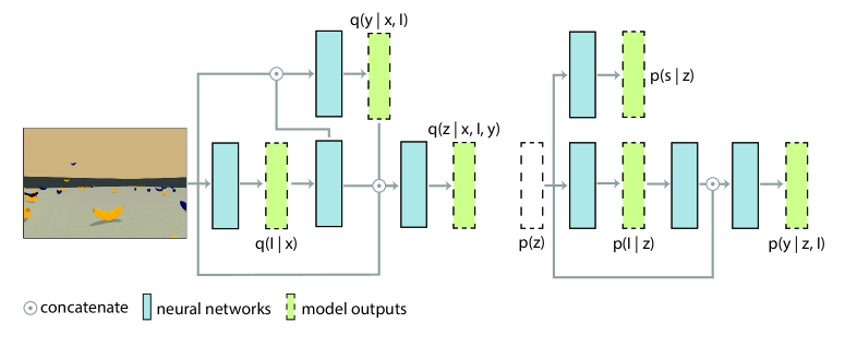
Figure 8: VCIQ architecture. The notation $i^{train}_{t}$ denotes the inference label available during training, whereas $\tilde{i}_{t}$ is sampled during causal variational inference as $i_{t}$ is unknown.

Appendix C C. Causal Effects

In a causal learning setting, evaluating treatment effects and conducting statistical refuting experiments are essential to support the underlying causal graphical model. Through resilient reinforcement learning framework, we could interpret DQN by estimating the average treatment effect (ATE) of each noisy and adversarial observation. We first define how to calculate a treatment effect in the resilient RL settings and conduct statistical refuting tests including random common cause variable test ($T_{c}$), replacing treatment with a random (placebo) variable ($T_{p}$), and removing a random subset of data ($T_{s}$). The open-source causal inference package Dowhy (Sharma, Kiciman et al. 2019) is used for analysis.

Average Treatment Effect under Intervention

We refine a Q-network with discrete actions for estimating treatment effects based on Theorem 1 in (Louizos et al. 2017). In particular, individual treatment effect (ITE) can be defined as the difference between the two potential outcomes of a Q-network; and the average treatment effect (ATE) is the expected value of the potential outcomes over the subjects. In a binary treatment setting, for a Q-value function $Q_{t}(s_{t})$ and the interfered state $\mathcal{I}(s_{t})$, the ITE and ATE are calculated by:

$$Q_{t}^{ITE}=Q_{t}(s_{t})\left(1-p_{t}\right)+Q_{t}({\mathcal{I}}(s_{t}))p_{t}$$ (14)

$$ATE=\sum_{t=1}^{\mathcal{T}}\frac{\mathbb{E}\left[Q_{t}^{ITE}({\mathcal{I}}(s_{t}))\right]-\mathbb{E}\left[Q_{t}^{ITE}(s_{t})\right]}{\mathcal{T}}$$ (15)

where $p_{t}$ is the estimated inference label by the agent and $\mathcal{T}$ is the total time steps of each episode. As expected, we find that CIQ indeed attains a better ATE and its significance can be informed by the refuting tests based on $T_{c}$, $T_{p}$ and $T_{s}$.

To evaluate the causal effect, we follow a standard refuting setting (Rothman and Greenland 2005; Pearl, Glymour, and Jewell 2016; Pearl 1995b) with the causal graphical model in Fig. 3 of the main context to run three major tests, as reported in Tab. 6. The code for the statistical test was conducted by Dowhy (Sharma, Kiciman et al. 2019), which has been submitted as supplementary material. (We intend to open source as a reproducible result.)

Pearl (Pearl 1995a) introduces a ”do-operator” to study this problem under intervention. The $do$ symbol removes the treatment $\mathbf{tr}$, which is equal to interference $\mathcal{I}$ in the Eq. (1) of the main content , from the given mechanism and sets it to a specific value by some external intervention. The notation $P(r_{t}|do(tr))$ denotes the probability of reward $r_{t}$ with possible interventions on treatment at time $t$. Following Pearl’s back-door adjustment formula (Pearl 2009) and the causal graphical model in Figure 2 of the main content., it is proved in (Louizos et al. 2017) that the causal effect for a given binary treatment $\mathbf{tr}$ (denoted as a binary interference label $i_{t}$ in Eq. (1) of the main content), a series of proxy variables $\mathbf{X}=(\sum^{\mathcal{T}}_{t=1}x_{t})\equiv\mathbf{S^{\prime}}=(\sum^{\mathcal{T}}_{t=1}s^{\prime}_{t}$), as $s^{\prime}_{t}$ in Eq. (1) of the main content, a summation of accumulated reward $\mathbf{R}=(\sum^{\mathcal{T}}_{t=1}\mathbf{r_{t}})$ and a confounding variable $\mathbf{Z}$ can be evaluated by (similarly for $\mathbf{tr}=0$):

$$\begin{array}[]{l}{p(\mathbf{R}|\mathbf{S^{\prime}},do(\mathbf{tr}=1))}=\int_{\mathbf{Z}}p(\mathbf{R}|\mathbf{S},do(\mathbf{tr}=1),\mathbf{Z})p(\mathbf{Z}|\mathbf{S},do(\mathbf{tr}=1))d\mathbf{Z}\stackrel{{\scriptstyle(i)}}{{=}}\\ \int_{\mathbf{Z}}p(\mathbf{R}|\mathbf{S^{\prime}},\mathbf{tr}=1,\mathbf{Z})p(\mathbf{Z}|\mathbf{S^{\prime}})d\mathbf{Z},\end{array}$$ (16)

where equality (i) is by the rules of do-calculus (Pearl 1995a; Pearl, Glymour, and Jewell 2016) applied to the causal graph applied on Figure 3 (a) of the main content. We extend to Eq. 16 on individual outcome study with DQNs, which is known by the Theorem 1. from Louizos et. al.  (Louizos et al. 2017) and Chapter 3.2 of Pearl (Pearl 2009).

Refutation Test:

A sampling plan for collecting samples refer to as subgroups (i=1, …, k). Common cause variation (T-c) is denoted as $\sigma_{c}$, which is an estimate of common cause variation within the subgroups in terms of the standard deviation of the within subgroup variation:

$$\sigma_{c}\cong\sum_{i=1}^{k}s_{i}/k,$$ (17)

where $k$ denotes as the number of sample size. We introduce intervention a error rate $n$, which is a probability to feed error interference (e.g., feed $i_{t}$ = 0 even under interference with a probability of $n$) and results shown in Table 5.

The test (T-p) of replacing treatment with a random (placebo) variable is conducted by modifying the graphical relationship in the proposed probabilistic model in Fig. 3 of the main context. The new assign variable will follow the placebo note but with a value sampling from a random Gaussian distribution. The test of removing a random subset of data (T-r) is to randomly split and sampling the subset value to calculate an average treatment value in the proposed graphical model. We use the official dowhy implementation, which includes: (1) confounders effect on treatment: how the simulated confounder affects the value of treatment; (2) confounders effect on outcome: how the simulated confounder affects the value of outcome; (3) effect strength on treatment: parameter for the strength of the effect of simulated confounder on treatment, and (4) effect strength on outcome: parameter for the strength of the effect of simulated confounder on outcome. Following the refutation experiment in the CEVAE paper, we conduct experiments shown in Tab. S5 and  S6 with 10 $\%$ to 50 $\%$ intervention noise on the binary treatment labels. The results in Tab. S5 show that proposed CIQ maintains a lower rate compared with the benchmark methods included logistic regression and CEVAE (refer to Fig. 4 (b) in (Louizos et al. 2017)).

Through Eq. (9) to (10) and the corresponding correct action rate in the main context, we could interpret deep q-network by estimating the average treatment effect (ATE) of each noisy and adversarial observation. ATE (Louizos et al. 2017; Shalit, Johansson, and Sontag 2017) is defined as the expected value of the potential outcomes (e.g., disease) over the subjects (e.g., clinical features.) For example, in navigation environments, we could rank the harmfulness of each noisy observation (Yang et al. 2019) against q-network from the autonomous driving agent.

Table 5: Absolute error ATE estimate; lower value indicates a much stable causal inference under perturbation on logic direction with $P^{I}=10\%$ and $n$=error rate of intervention on the binary label.

Model	$n$=0.1	$n$=0.2	$n$=0.3	$n$=0.4	$n$=0.5
LR	0.062	0.084	0.128	0.151	0.164
CEVAE	0.021	0.042	0.062	0.072	0.081
CIQ	0.019	0.020	0.015	0.018	0.023

Table 6: Validation of causal effect by three causal refuting tests. The causal effect estimate is tested by random common cause variable test (T-c), replacing treatment with a random (placebo) variable (T-p – lower is better), and removing a random subset of data (T-r). Adversarial attack outperforms in most tests.

Noise : $do(\mathcal{I})$ n = 0.1 n = 0.2 Method ATE w/ T-c w/ T-p w/ T-s ATE w/ T-c w/ T-p w/ T-s Adversarial 0.2432 0.2431 0.0294 0.2488 0.0868 0.0868 0.0109 0.0865 Black-out 0.2354 0.2212 0.0244 0.2351 0.0873 0.0870 0.0140 0.0781 Gaussian 0.1792 0.1763 0.0120 0.1751 0.0590 0.0610 0.0130 0.0571 Frozen Frame 0.1614 0.1614 0.0168 0.1435 0.0868 0.0868 0.0140 0.0573

Appendix D D. Ablation Studies

The Number of Model Parameters

We also spend efforts on a parameter-study on the results of average returns between different DQN-based models, which included DQN, Double DQN (DDQN), DDQN with dueling, CIQ, DQN with a classifier (DQN-CF), DDQN with a classifier (DDQN-CF), DQN with a variational autoencoder (Kingma and Welling 2013) (DQN-VAE), NoisyNet, and using the latent input of causal effect variational autoencoder for Q network (CEVAE-Q) prediction. Overall, CEVAE-Q is with minimal-requested parameters with 14.4 M (in Env₁) as the largest model used in our experiments in Tab. 7. CIQ remains roughly similar parameters as 9.7M compared with DDQN, DDQN_d, and Noisy Net. Our ablation study in Tab. 7 indicates the advantages of CIQ are not owing to extensive features using in the model according to the size of parameters. CIQ attains benchmark results in our resilient reinforcement learning setting compared to the other DQN models.

Table 7: Ablation study on parameter of different DQN models using in our experiments in Env₁, Env₂, Env₃, and Env₄.

Model	Para.	Env1	Env2	Env3	Env4
DQN	6.9M	20.2	3.1	-113.6	10.8
DDQN	9.7M	41.1	3.5	-123.4	57.9
DDQNd	9.7M	82.9	4.7	-136.3	67.2
CIQ	9.7M	195.1	12.5	200.1	195.2
DQN-CF	9.7M	140.5	12.5	-78.3	120.2
DDQN-CF	12.1M	161.3	12.5	-10.1	128.2
DQN-VAE	9.7M	151.1	7.6	-92.9	24.1
NoisyNet	9.7M	158.6	5.5	50.1	100.1
CEVAE-Q	12.5M	39.8	11.5	-156.5	45.8
DVRLQ-CF	10.7M	107.11	9.2	-34.9	42.5

Noisy Nets (Fortunato et al. 2018) has been introduced as a benchmark whose parameters are perturbed by a parametric noise function. We select Noisy Net in a DQN format as a noisy training baseline with interfered state $s^{\prime}_{t}$ concated with a interference label $i_{t}$ from a classifier.

Latent Representations

We conduct an ablation study by comparing other latent representation methods to the proposed CIQ model.

DQN with an variational autoencoder (DQN-VAE): To learn important features from observations, many recent works leverage deep variational inference for accessing latent states for feeding into DQN. We provide a baseline on training a variational autoencoder (VAE) built upon the DQN baseline, denoted as DQN-VAE. The DQN-VAE baseline is targeted to recover a potential noisy state and feed the bottleneck latent features into the Q-network.

CEVAE-Q Network: TARNet (Shalit, Johansson, and Sontag 2017; Louizos et al. 2017) is a major class of neural network architectures for estimating outcomes of a binary treatment on linear data (e.g., clinical reports). Our proposed CIQ uses an end-to-end approach to learn the interventional (causal) features. We provide another baseline on using the latent features from a causal variational autoencoder (Louizos et al. 2017) (CEVAE) as latent features as state inputs followed the loss function in (Louizos et al. 2017). To get the causal latent model in Q-network, we approximate the posterior distribution by a neural network $z_{t}\sim p(z_{t}|\tilde{x}_{t})=\phi(\tilde{x}_{t};\theta_{1})$. Then we train this neural network, CEVAE-Q, by variational inference using the generative model.

We conduct 10,000 times experiments and fine-tuning on DQN-VAE and CEVAE-Q. The results in Table 8 shows that the latent representation learned by CIQ provides better resilience than other representations.

Table 8: Performance on average return in clean and five different noise level in Env₁ evaluated by an average of under uncertain perturbation included Gaussian, adversarial, blackout, and frozen frame. All DQN models solve the environment with over 195.0 average returns in a clean state input (a.k.a. no noise).

Model	0%	10%	20%	30%	40%	50%	Cosine	Para.
DQN	195.1	115.0	68.9	32.3	22.8	19.1	42.1	6.9 M
DDQN	195.1	123.4	73.2	59.4	28.1	22.8	62.8	9.7 M
CIQ	195.1	195.1	195.1	195.0	168.2	113.1	195.0	9.7 M
DQN-VAE	195.1	173.5	141.3	124.8	86.5	33.3	101.2	9.7 M
DQN-CEVAE	195.1	154.4	111.9	94.8	75.5	48.3	82.1	12.5 M

Table 9: Structure-wise ablation studies of CIQ in Env₁ (noise level $P=20\%$).

Model	Return	CLEVER-Q	AC-Rate
CIQ	195.1	0.241	97.3
B1: CIQ w/o the concatenation	152.1	0.196	78.2
B2: CIQ w/o the $\theta_{3}$ network	150.1	0.182	65.6
B3: CIQ w/o providing grounded $i_{t}$ for training	135.1	0.142	53.6

Architecture Ablation Study on CIQ

To study the importance of specific components in CIQ, we conducted additional ablation studies and constructed two new baseline models shown in Table 9 tested in Env₁ (Cartpole). Baseline 1 (B1) - CIQ w/o the concatenation of $\tilde{i}_{t}$ in $S^{C}_{I}$. This comparison shows the importance of using both the predicted confounder $\tilde{z}_{t}$ and the predicted label $\tilde{i}_{t}$. B1 uses label prediction to help latent representation but not using the predicted labels in decision-making. The structure is motivated by a task-specific (depth-only information from a maze environment) DQN network from a previous study (Mirowski et al. 2016).

Baseline 2 (B2) - CIQ w/o the $\theta_{3}$ network (for testing $\theta_{3}$’s importance).

Baseline 3 (B3) - CIQ w/o providing grounded $i_{t}$ for training, for testing the importance of the inference loss and joint loss propagation. The superior performance of CIQ validates the proposed model is indeed crucial from the previous discussion in Section 3 of the main content.The setting used for Table 16 is the same as the setting for the third column (noise level = 20%) in Table 5 and the third column (noise level = 20%) in Table 15, tested in Env₁ (Cartpole).

We provide another variant of DQN-CF with “two heads” to account for the binary classifier output (perturbed/non-perturbed). We conduct experiments in Env₁ with Gaussian interference ($\mathcal{I}$=L₂) for this two-head DQN-CF variant, denoted as DQN-CF2H.

As shown in Tab. 10, DQN-CF2H achieves slightly better performance than DQN-CF at the higher noise levels P=$\{30\%,40\%\}$, but slightly worse performance at the lower noise levels P=$\{10\%,20\%\}$. CIQ still performs the best in terms of average rewards and CLEVER-Q scores, suggesting the benefits of our method beyond the architectural difference.

Table 10: Evaluation of $\{$average rewards$/$CLEVER-Q$\}$ in Env₁.

Model, $\mathcal{I}$=L2	P=10%	P=20%	P=30%	P=40%
DQN-CF	192.8$/$0.185	147.7$/$0.145	131.4$/$0.127	88.2$/$0.92
DQN-CF2H	188.4$/$0.180	145.2$/$0.141	135.2$/$0.131	92.1$/$0.97
CIQ	195.1$/$0.221	195.1$/$0.235	195.0$/$0.232	168.2$/$0.186

Perturbation-based Neural Saliency for DQN Agents

To better understand our CIQ model, we use the benchmark saliency method on DQN agent, perturbation-based saliency map, (Greydanus et al. 2018) to visualize the salient pixels, which are sensitive to the loss function of the trained DQNs. We made a case study of an input frame under an adversarial perturbation, as shown in Fig. 7. We evaluate DQN agents included DQN, CIQ, DQN-CF, DVRLQ-CF and record its weighted center from the neural saliency map, where saliency pixels of CIQ respond to ground true actions more frequent (96.2%) than the other DQN methods.

Predicted interference label accuracy: We use the switching mechanism for end-to-end DQN training. The major difference between CIQ and enhanced DQNs is how to use the interference information for learning, which results in different architectures. We provide a related case study in Table 11. Considerall the task and noisy conditions, the Pearson correlation coefficient between prediction accuracy and average returns is 0.1081, which shows low statistical correlation.

Baselines discussion considering the variance of average rewards: We follow the standard DQNs performance evaluation in the DRL community by using average returns to evaluate the performance for DQNs. CIQ’s average returns outperform the other DQNs. Moreover, CIQ shows advantage on evaluated robustness properties including CLEVER-Q and action correction rate. We calculate the p-value of the learning curves of CIQ between the other DQNs over all evaluated noisy conditions and environments. In general, the p-value ¡0.05 could be considered as statistically significant in Table 12.

White-out Ablation: We tested the performance of CIQ against unseen (not used int raining) interferences and showed that CIQ has improved robustness. In our white experiments, from scratch training with white-out perturbation, CIQ remains the best in all deployed environments. The average reward for white-out (e.g., to give each state observation a max-available intensity) agents showed a relative 12.3% decay from black-out perturbation (e.g., set each state observation as zero).

Table 11: Additional ablation study with noisy environments (P= 20%) for (continuous control Cartpole).The number shows prediction accuracy on the interference label (%).

Model	Gaussian	Adversarial	Blackout	Frozen
DQN-CF	98.34	95.34	100.00	91.23
DVRLQ-CF	97.34	95.52	100.00	90.92
CIQ	98.21	95.67	100.00	90.82

Table 12: p-value of the learning curves collected different environments and noisy types and levels presented in this paper. The results suggested that the learning curves of CIQs (best performance in terms of the average returns, CLEVER-Q, action correction rate) could be considered as statistically significant.

Model	DQN	DQN-CF	DQN-SA	DVRLQ	DVRLQ-CF
CIQ	0.0112	0.0291	0.0212	0.0142	0.0183

Robustness Transferability among Different Interference Types

We conduct additional experiments to study robustness transferability of DQN and CIQ when training and testing under different kinds of interference types in Env₁. Note that both architectures would solve a clean environment successfully (over 195.0). The reported numbers are averaged over 20 independent runs for each condition. As shown in Table 13 and Table 14, CIQ agents consistently attain significant performance improvement when compared with DQN agents, especially between Gaussian and adversarial perturbation. For example, CIQ succeeded to solve the environment 12 times out of 20 independent runs, with an average score of 165.2 in Gaussian (train)-Adversarial (test) adaptation. n particular, for CIQ, 12 times out of 20 independent runs are successfully transfered from Gaussian to Adversarial perturbation. Interestingly, augmenting adversarial perturbation does not always guarantee the best policy transfer when testing in the Blackout and Frozen conditions, which shows a slightly lower performance compared with training on Gaussian interference. The reason could be attributed to the recent findings that adversarial training can undermine model generalization (Raghunathan et al. 2019; Su et al. 2018).

Table 13: DQN adaptation: train and test on different interference (noise level $P=20\%$) in Env₁.

Train / Test	Gaussian	Adversarial	Blackout	Frozen
Gaussian	67.4	38.4	43.7	52.1
Adversarial	53.2	42.5	35.3	44.2
Blackout	46.2	27.4	85.7	50.3
Frozen	62.3	26.2	45.9	62.1

Table 14: CIQ adaptation: train and test on different interference (noise level $P=20\%$) in Env₁.

Train / Test	Gaussian	Adversarial	Blackout	Frozen
Gaussian	195.1	165.2	158.2	167.8
Adversarial	162.8	195.0	152.4	162.5
Blackout	131.3	121.1	195.3	145.7
Frozen	161.6	135.8	147.1	195.2

CIQ with Multi-Interference.

Here we show how the proposed CIQ model can be extended from the architecture shown in Figure 4 to the multi-interference (MI) setting. The design intuition is based on two-step inference by a common encoder, to infer a clean or noisy observation, followed by an individual decoder tied to an interference type, to infer noisy types and activate the corresponding Q-network (named $\theta_{4}$).
Note that the two-step inference mechanism follows the RCM as two sequential potential outcome estimation models (Rubin 1974; Imbens and Rubin 2010), where interfered observation $x^{\prime}_{t}$ is determined by two labels $i_{1,t}$ and $i_{2,t}$ according to $x^{\prime}_{t}=i_{1,t}(i_{2,t}\mathcal{I}_{1}(x_{t})+(1-i_{2,t})\mathcal{I}_{2}(x_{t}))+(1-i_{1,t})x_{t}$ extended from Eq.(1), where $i_{1,t}$ indicates the presence of interference and $i_{2,t}$ indicates which interference type (here we show the case of two types). As a proof of concept, we consider two interference types together, Gaussian noise and adversarial perturbation. In this setting every observation (state) can possibly undergo an interference with either Gaussian noise or Adversarial perturbation. From the results shown in Table. 3, we find that the extended version of CIQ, CIQ-MI, is capable of making correct action to solve (over 195.0) the environment when training with mixed interference types (last row). Another finding is that robustness tranferability (153.9/154.2) in CIQ-MI is slightly degraded compared to the results (162.8/165.2) in Table 14 with the same training episodes ($500$) and runs ($20$), which could be caused by the increased requirement of model capacity (Ammanabrolu and Riedl 2019; Yang et al. 2020a) of CIQ-MI.

Hardware Setup and Energy Cost

We use Nvidia GPUs (2080-Ti and V100) for our experiments with Compute Unified Device Architecture (CUDA) version 10.1. To conduct the results shown in the paper, it takes around 20 min to run 1,000 epochs (maximum) with a batch size 32 for each environment considering the hyper-parameters tuning described in Section B of the main paper. In total, the experiments presented (four environment with four different types of noise and its ablation studies) in this paper took around 343 wall-clock hours with a 300W power supplier.

Broader Impact

With the recent advances in using (deep) RL to solve problems that were once believed to be challenging for machines to learn and understand, we believe it is timely to move to the next milestone: understanding the resilience of DRL to rare but possible and recurring noisy interferences, which motivates this work with a novel deign of Q-networks inspired from causal learning.

• Who may benefit from this research: Researchers working on RL technology; as well as the users using the related technology for responsible and safe machine learning technology.

• Who may be put at disadvantage from this research: : When the work discloses the findings that Q-networks can be sensitive to noisy interferences, we understand the responsibilities of explaining the results to the public properly and providing reproducible evaluation.

• Whether the task/method leverages biases in the data: To alleviate possible bias in the data and model, we put efforts toward designing reproducible metrics and evaluating a wide variety of reproducible environments, interference types, and several baseline models.

References

- Alshiekh et al. (2018) Alshiekh, M.; Bloem, R.; Ehlers, R.; Könighofer, B.; Niekum, S.; and Topcu, U. 2018. Safe reinforcement learning via shielding. In Thirty-Second AAAI Conference on Artificial Intelligence.
- Ammanabrolu and Riedl (2019) Ammanabrolu, P.; and Riedl, M. 2019. Transfer in Deep Reinforcement Learning Using Knowledge Graphs. In Proceedings of the Thirteenth Workshop on Graph-Based Methods for Natural Language Processing (TextGraphs-13), 1–10.
- Bareinboim, Forney, and Pearl (2015) Bareinboim, E.; Forney, A.; and Pearl, J. 2015. Bandits with unobserved confounders: A causal approach. In Advances in Neural Information Processing Systems, 1342–1350.
- Bengio (2013) Bengio, Y. 2013. Deep learning of representations: Looking forward. In International Conference on Statistical Language and Speech Processing, 1–37. Springer.
- Bennett et al. (2021) Bennett, A.; Kallus, N.; Li, L.; and Mousavi, A. 2021. Off-policy evaluation in infinite-horizon reinforcement learning with latent confounders. In International Conference on Artificial Intelligence and Statistics, 1999–2007. PMLR.
- Brockman et al. (2016) Brockman, G.; Cheung, V.; Pettersson, L.; Schneider, J.; Schulman, J.; Tang, J.; and Zaremba, W. 2016. Openai gym. arXiv preprint arXiv:1606.01540.
- Dabney et al. (2018) Dabney, W.; Rowland, M.; Bellemare, M. G.; and Munos, R. 2018. Distributional reinforcement learning with quantile regression. In Thirty-Second AAAI Conference on Artificial Intelligence.
- Dhariwal et al. (2017) Dhariwal, P.; Hesse, C.; Klimov, O.; Nichol, A.; Plappert, M.; Radford, A.; Schulman, J.; Sidor, S.; Wu, Y.; and Zhokhov, P. 2017. OpenAI Baselines. https://github.com/openai/baselines.
- Dulac-Arnold et al. (2012) Dulac-Arnold, G.; Denoyer, L.; Preux, P.; and Gallinari, P. 2012. Fast reinforcement learning with large action sets using error-correcting output codes for mdp factorization. In Joint European Conference on Machine Learning and Knowledge Discovery in Databases, 180–194. Springer.
- Everett (2021) Everett, M. 2021. Neural Network Verification in Control. arXiv preprint arXiv:2110.01388.
- Forney, Pearl, and Bareinboim (2017) Forney, A.; Pearl, J.; and Bareinboim, E. 2017. Counterfactual data-fusion for online reinforcement learners. In International Conference on Machine Learning, 1156–1164.
- Fortunato et al. (2018) Fortunato, M.; Azar, M. G.; Piot, B.; Menick, J.; Osband, I.; Graves, A.; Mnih, V.; Munos, R.; Hassabis, D.; Pietquin, O.; et al. 2018. Noisy networks for exploration. ICLR 2018, arXiv preprint arXiv:1706.10295.
- Fox, Pakman, and Tishby (2015) Fox, R.; Pakman, A.; and Tishby, N. 2015. Taming the noise in reinforcement learning via soft updates. arXiv preprint arXiv:1512.08562.
- Franklin et al. (1998) Franklin, G. F.; Powell, J. D.; Workman, M. L.; et al. 1998. Digital control of dynamic systems, volume 3. Addison-wesley Menlo Park, CA.
- Goodfellow, Shlens, and Szegedy (2015) Goodfellow, I. J.; Shlens, J.; and Szegedy, C. 2015. Explaining and harnessing adversarial examples. ICLR.
- Greenland, Pearl, and Robins (1999) Greenland, S.; Pearl, J.; and Robins, J. M. 1999. Causal diagrams for epidemiologic research. Epidemiology, 37–48.
- Gregor et al. (2018) Gregor, K.; Papamakarios, G.; Besse, F.; Buesing, L.; and Weber, T. 2018. Temporal difference variational auto-encoder. arXiv preprint arXiv:1806.03107.
- Greydanus et al. (2018) Greydanus, S.; Koul, A.; Dodge, J.; and Fern, A. 2018. Visualizing and Understanding Atari Agents. In International Conference on Machine Learning, 1792–1801.
- Grigorescu et al. (2020) Grigorescu, S.; Trasnea, B.; Cocias, T.; and Macesanu, G. 2020. A survey of deep learning techniques for autonomous driving. Journal of Field Robotics, 37(3): 362–386.
- Gu et al. (2017) Gu, S.; Holly, E.; Lillicrap, T.; and Levine, S. 2017. Deep reinforcement learning for robotic manipulation with asynchronous off-policy updates. In 2017 IEEE international conference on robotics and automation (ICRA), 3389–3396. IEEE.
- Ha and Schmidhuber (2018) Ha, D.; and Schmidhuber, J. 2018. World models. arXiv preprint arXiv:1803.10122.
- Hafner et al. (2018) Hafner, D.; Lillicrap, T.; Fischer, I.; Villegas, R.; Ha, D.; Lee, H.; and Davidson, J. 2018. Learning latent dynamics for planning from pixels. arXiv preprint arXiv:1811.04551.
- Harutyunyan et al. (2016) Harutyunyan, A.; Bellemare, M. G.; Stepleton, T.; and Munos, R. 2016. Q lamda with Off-Policy Corrections. In International Conference on Algorithmic Learning Theory, 305–320. Springer.
- Helwegen, Louizos, and Forré (2020) Helwegen, R.; Louizos, C.; and Forré, P. 2020. Improving Fair Predictions Using Variational Inference In Causal Models. arXiv preprint arXiv:2008.10880.
- Higgins et al. (2018) Higgins, I.; Amos, D.; Pfau, D.; Racaniere, S.; Matthey, L.; Rezende, D.; and Lerchner, A. 2018. Towards a definition of disentangled representations. arXiv preprint arXiv:1812.02230.
- Huang et al. (2017) Huang, S.; Papernot, N.; Goodfellow, I.; Duan, Y.; and Abbeel, P. 2017. Adversarial attacks on neural network policies. arXiv preprint arXiv:1702.02284.
- Igl et al. (2018) Igl, M.; Zintgraf, L.; Le, T. A.; Wood, F.; and Whiteson, S. 2018. Deep Variational Reinforcement Learning for POMDPs. In International Conference on Machine Learning, 2117–2126.
- Imbens and Rubin (2010) Imbens, G. W.; and Rubin, D. B. 2010. Rubin causal model. In Microeconometrics, 229–241. Springer.
- Jaber, Zhang, and Bareinboim (2019) Jaber, A.; Zhang, J.; and Bareinboim, E. 2019. Causal identification under markov equivalence: Completeness results. In International Conference on Machine Learning, 2981–2989.
- Jaderberg et al. (2017) Jaderberg, M.; Mnih, V.; Czarnecki, W. M.; Schaul, T.; Leibo, J. Z.; Silver, D.; and Kavukcuoglu, K. 2017. Reinforcement learning with unsupervised auxiliary tasks. ICLR.
- Johansen et al. (2015) Johansen, T. A.; Cristofaro, A.; Sørensen, K.; Hansen, J. M.; and Fossen, T. I. 2015. On estimation of wind velocity, angle-of-attack and sideslip angle of small UAVs using standard sensors. In 2015 International Conference on Unmanned Aircraft Systems (ICUAS), 510–519. IEEE.
- Juliani et al. (2018) Juliani, A.; Berges, V.-P.; Vckay, E.; Gao, Y.; Henry, H.; Mattar, M.; and Lange, D. 2018. Unity: A general platform for intelligent agents. arXiv preprint arXiv:1809.02627.
- Jung, Tian, and Bareinboim (2021) Jung, Y.; Tian, J.; and Bareinboim, E. 2021. Estimating identifiable causal effects through double machine learning. In Proceedings of the 35th AAAI Conference on Artificial Intelligence.
- Kaelbling, Littman, and Cassandra (1998) Kaelbling, L. P.; Littman, M. L.; and Cassandra, A. R. 1998. Planning and acting in partially observable stochastic domains. Artificial intelligence, 101(1-2): 99–134.
- Kalashnikov et al. (2018) Kalashnikov, D.; Irpan, A.; Pastor, P.; Ibarz, J.; Herzog, A.; Jang, E.; Quillen, D.; Holly, E.; Kalakrishnan, M.; Vanhoucke, V.; et al. 2018. Qt-opt: Scalable deep reinforcement learning for vision-based robotic manipulation. arXiv preprint arXiv:1806.10293.
- Khemakhem et al. (2021) Khemakhem, I.; Monti, R.; Leech, R.; and Hyvarinen, A. 2021. Causal autoregressive flows. In International Conference on Artificial Intelligence and Statistics, 3520–3528. PMLR.
- Killian, Ghassemi, and Joshi (2020) Killian, T. W.; Ghassemi, M.; and Joshi, S. 2020. Counterfactually Guided Policy Transfer in Clinical Settings. arXiv preprint arXiv:2006.11654.
- Kingma and Ba (2014) Kingma, D. P.; and Ba, J. 2014. Adam: A method for stochastic optimization. arXiv preprint arXiv:1412.6980.
- Kingma and Welling (2013) Kingma, D. P.; and Welling, M. 2013. Auto-encoding variational bayes. arXiv preprint arXiv:1312.6114.
- Lee et al. (2018) Lee, G.; Hou, B.; Mandalika, A.; Lee, J.; Choudhury, S.; and Srinivasa, S. S. 2018. Bayesian policy optimization for model uncertainty. arXiv preprint arXiv:1810.01014.
- Lin et al. (2017) Lin, Y.-C.; Hong, Z.-W.; Liao, Y.-H.; Shih, M.-L.; Liu, M.-Y.; and Sun, M. 2017. Tactics of adversarial attack on deep reinforcement learning agents. arXiv preprint arXiv:1703.06748.
- Louizos et al. (2017) Louizos, C.; Shalit, U.; Mooij, J. M.; Sontag, D.; Zemel, R.; and Welling, M. 2017. Causal effect inference with deep latent-variable models. In Advances in Neural Information Processing Systems, 6446–6456.
- Lu, Schölkopf, and Hernández-Lobato (2018) Lu, C.; Schölkopf, B.; and Hernández-Lobato, J. M. 2018. Deconfounding reinforcement learning in observational settings. arXiv preprint arXiv:1812.10576.
- Lynch et al. (2020) Lynch, C.; Khansari, M.; Xiao, T.; Kumar, V.; Tompson, J.; Levine, S.; and Sermanet, P. 2020. Learning latent plans from play. In Conference on Robot Learning, 1113–1132. PMLR.
- Madumal et al. (2020) Madumal, P.; Miller, T.; Sonenberg, L.; and Vetere, F. 2020. Explainable reinforcement learning through a causal lens. In Proceedings of the AAAI Conference on Artificial Intelligence, volume 34, 2493–2500.
- Mirowski et al. (2016) Mirowski, P.; Pascanu, R.; Viola, F.; Soyer, H.; Ballard, A. J.; Banino, A.; Denil, M.; Goroshin, R.; Sifre, L.; Kavukcuoglu, K.; et al. 2016. Learning to navigate in complex environments. arXiv preprint arXiv:1611.03673.
- Mnih et al. (2016) Mnih, V.; Badia, A. P.; Mirza, M.; Graves, A.; Lillicrap, T.; Harley, T.; Silver, D.; and Kavukcuoglu, K. 2016. Asynchronous methods for deep reinforcement learning. In International conference on machine learning, 1928–1937.
- Mnih et al. (2015) Mnih, V.; Kavukcuoglu, K.; Silver, D.; Rusu, A. A.; Veness, J.; Bellemare, M. G.; Graves, A.; Riedmiller, M.; Fidjeland, A. K.; Ostrovski, G.; et al. 2015. Human-level control through deep reinforcement learning. Nature, 518(7540): 529.
- Moreno et al. (2018) Moreno, P.; Humplik, J.; Papamakarios, G.; Pires, B. A.; Buesing, L.; Heess, N.; and Weber, T. 2018. Neural belief states for partially observed domains. In NeurIPS 2018 workshop on Reinforcement Learning under Partial Observability.
- Nagabandi et al. (2018) Nagabandi, A.; Clavera, I.; Liu, S.; Fearing, R. S.; Abbeel, P.; Levine, S.; and Finn, C. 2018. Learning to adapt in dynamic, real-world environments through meta-reinforcement learning. arXiv preprint arXiv:1803.11347.
- Osband et al. (2019) Osband, I.; Doron, Y.; Hessel, M.; Aslanides, J.; Sezener, E.; Saraiva, A.; McKinney, K.; Lattimore, T.; Szepezvari, C.; Singh, S.; et al. 2019. Behaviour suite for reinforcement learning. arXiv preprint arXiv:1908.03568.
- Papadimitriou and Tsitsiklis (1987) Papadimitriou, C. H.; and Tsitsiklis, J. N. 1987. The complexity of Markov decision processes. Mathematics of operations research, 12(3): 441–450.
- Pearl (1995a) Pearl, J. 1995a. Causal diagrams for empirical research. Biometrika, 82(4): 669–688.
- Pearl (1995b) Pearl, J. 1995b. On the testability of causal models with latent and instrumental variables. In Proceedings of the Eleventh conference on Uncertainty in artificial intelligence, 435–443. Morgan Kaufmann Publishers Inc.
- Pearl (2009) Pearl, J. 2009. Causality. Cambridge university press.
- Pearl (2019) Pearl, J. 2019. The seven tools of causal inference, with reflections on machine learning. Communications of the ACM, 62(3): 54–60.
- Pearl, Glymour, and Jewell (2016) Pearl, J.; Glymour, M.; and Jewell, N. P. 2016. Causal inference in statistics: A primer. John Wiley & Sons.
- Raghunathan et al. (2019) Raghunathan, A.; Xie, S. M.; Yang, F.; Duchi, J. C.; and Liang, P. 2019. Adversarial training can hurt generalization. arXiv preprint arXiv:1906.06032.
- Robins, Rotnitzky, and Zhao (1995) Robins, J. M.; Rotnitzky, A.; and Zhao, L. P. 1995. Analysis of semiparametric regression models for repeated outcomes in the presence of missing data. Journal of the american statistical association, 90(429): 106–121.
- Rothman and Greenland (2005) Rothman, K. J.; and Greenland, S. 2005. Causation and causal inference in epidemiology. American journal of public health, 95(S1): S144–S150.
- Rubin (1974) Rubin, D. B. 1974. Estimating causal effects of treatments in randomized and nonrandomized studies. Journal of educational Psychology, 66(5): 688.
- Saunders et al. (2018) Saunders, W.; Sastry, G.; Stuhlmueller, A.; and Evans, O. 2018. Trial without error: Towards safe reinforcement learning via human intervention. In Proceedings of the 17th International Conference on Autonomous Agents and MultiAgent Systems, 2067–2069. International Foundation for Autonomous Agents and Multiagent Systems.
- Schmidhuber (1991) Schmidhuber, J. 1991. Reinforcement learning in Markovian and non-Markovian environments. In Advances in neural information processing systems, 500–506.
- Schmidhuber (1992) Schmidhuber, J. 1992. Learning complex, extended sequences using the principle of history compression. Neural Computation, 4(2): 234–242.
- Shalit, Johansson, and Sontag (2017) Shalit, U.; Johansson, F. D.; and Sontag, D. 2017. Estimating individual treatment effect: generalization bounds and algorithms. In Proceedings of the 34th International Conference on Machine Learning-Volume 70, 3076–3085. JMLR. org.
- Sharma, Kiciman et al. (2019) Sharma, A.; Kiciman, E.; et al. 2019. DoWhy A Python package for causal inference. KDD 2019 workshop.
- Silver et al. (2017) Silver, D.; Schrittwieser, J.; Simonyan, K.; Antonoglou, I.; Huang, A.; Guez, A.; Hubert, T.; Baker, L.; Lai, M.; Bolton, A.; et al. 2017. Mastering the game of Go without human knowledge. Nature, 550(7676): 354.
- Su et al. (2018) Su, D.; Zhang, H.; Chen, H.; Yi, J.; Chen, P.-Y.; and Gao, Y. 2018. Is robustness the cost of accuracy?–a comprehensive study on the robustness of 18 deep image classification models. In ECCV, 631–648.
- Sutton et al. (1998) Sutton, R. S.; Barto, A. G.; Bach, F.; et al. 1998. Reinforcement learning: An introduction. MIT press.
- Szegedy et al. (2014) Szegedy, C.; Zaremba, W.; Sutskever, I.; Bruna, J.; Erhan, D.; Goodfellow, I.; and Fergus, R. 2014. Intriguing properties of neural networks. International Conference on Learning Representations.
- Tai, Paolo, and Liu (2017) Tai, L.; Paolo, G.; and Liu, M. 2017. Virtual-to-real deep reinforcement learning: Continuous control of mobile robots for mapless navigation. In 2017 IEEE/RSJ International Conference on Intelligent Robots and Systems (IROS), 31–36. IEEE.
- Tennenholtz, Mannor, and Shalit (2019) Tennenholtz, G.; Mannor, S.; and Shalit, U. 2019. Off-Policy Evaluation in Partially Observable Environments. arXiv preprint arXiv:1909.03739.
- Van Hasselt, Guez, and Silver (2016) Van Hasselt, H.; Guez, A.; and Silver, D. 2016. Deep reinforcement learning with double q-learning. In Thirtieth AAAI conference on artificial intelligence.
- Weng et al. (2018) Weng, T.-W.; Zhang, H.; Chen, P.-Y.; Yi, J.; Su, D.; Gao, Y.; Hsieh, C.-J.; and Daniel, L. 2018. Evaluating the robustness of neural networks: An extreme value theory approach. arXiv preprint arXiv:1801.10578.
- Yan, Xu, and Liu (2016) Yan, C.; Xu, W.; and Liu, J. 2016. Can you trust autonomous vehicles: Contactless attacks against sensors of self-driving vehicle. DEFCON24.
- Yang et al. (2020a) Yang, C.-H. H.; Liu, L.; Gandhe, A.; Gu, Y.; Raju, A.; Filimonov, D.; and Bulyko, I. 2020a. Multi-task Language Modeling for Improving Speech Recognition of Rare Words. arXiv preprint arXiv:2011.11715.
- Yang et al. (2019) Yang, C.-H. H.; Liu, Y.-C.; Chen, P.-Y.; Ma, X.; and Tsai, Y.-C. J. 2019. When causal intervention meets adversarial examples and image masking for deep neural networks. In 2019 IEEE International Conference on Image Processing (ICIP), 3811–3815. IEEE.
- Yang et al. (2020b) Yang, C.-H. H.; Qi, J.; Chen, P.-Y.; Ouyang, Y.; Hung, I.-T. D.; Lee, C.-H.; and Ma, X. 2020b. Enhanced Adversarial Strategically-Timed Attacks Against Deep Reinforcement Learning. In ICASSP 2020-2020 IEEE International Conference on Acoustics, Speech and Signal Processing (ICASSP), 3407–3411. IEEE.
- Yurtsever et al. (2020) Yurtsever, E.; Lambert, J.; Carballo, A.; and Takeda, K. 2020. A survey of autonomous driving: Common practices and emerging technologies. IEEE Access, 8: 58443–58469.
- Zhang et al. (2020) Zhang, A.; Lyle, C.; Sodhani, S.; Filos, A.; Kwiatkowska, M.; Pineau, J.; Gal, Y.; and Precup, D. 2020. Invariant causal prediction for block mdps. In International Conference on Machine Learning, 11214–11224. PMLR.
- Zhang, Zhang, and Li (2020) Zhang, C.; Zhang, K.; and Li, Y. 2020. A Causal View on Robustness of Neural Networks. Advances in Neural Information Processing Systems, 33.
- Zhang and Bareinboim (2020) Zhang, J.; and Bareinboim, E. 2020. Designing optimal dynamic treatment regimes: A causal reinforcement learning approach. In International Conference on Machine Learning, 11012–11022. PMLR.
- Zhang and Bareinboim (2021) Zhang, J.; and Bareinboim, E. 2021. Bounding Causal Effects on Continuous Outcome. In Proceedings of the 35nd AAAI Conference on Artificial Intelligence.
- Zhang, Kumor, and Bareinboim (2020) Zhang, J.; Kumor, D.; and Bareinboim, E. 2020. Causal imitation learning with unobserved confounders. Advances in Neural Information Processing Systems, 33.