Gyrating solitons in a necklace of optical waveguides

Abstract

We consider light pulses in a circular array of $2N$ coupled nonlinear optical waveguides. The waveguides are either hermitian or alternate gain and loss in a $\mathcal{PT}$-symmetric fashion. Simple patterns in the array include a ring of $2N$ pulses travelling abreast, and a breather — a string of pulses where all even and all odd waveguides flash in turn. In addition, the structure displays solitons gyrating around the necklace by switching from one waveguide to the next. Some of the gyrating solitons are stable while other ones are weakly unstable and evolve into gyrating multiflash strings. By tuning the gain-loss coefficient, the gyration of solitons in a nonhermitian array may be reversed without changing the direction of their translational motion.

I Introduction

The uses of nonlinear fibre arrays for the all-optical signal processing have been recognised since the late 1980s. The multiple channel waveguide couplers and multicore fibres can be utilised for light switching switch ; Krolikowski , power dividing Hudg , beam shaping beam_shaping , discrete diffraction management Longhi , spatial-division multiplexing multiplex , coherent beam combination and optical pulse compression Aceves . In recent years interest has been shifting to low-dimensional arrays, typically arranged in a ring ring ; Chekh . New applications of circular arrays include vortex switching schemes Alexeyev ; vortices and generation of light beams carrying orbital angular momentum OAM .

Studies of coupled waveguides have received a new impetus with the advent of the parity-time symmetry. Originally proposed in the context of the nonhermitian quantum mechanics PT , the $\mathcal{PT}$-symmetry proved to furnish a set of rules for the inclusion of gain and loss in fiber arrays PTwaveguide and photonic lattices PTphot . The nonhermitian optics provides light-control opportunities unattainable with traditional set-ups, including low-threshold switching PTwaveguide ; SXK and unidirectional invisibility PTwaveguide ; Lin .

A circular array of waveguides is an ideal platform for the $\mathcal{PT}$-symmetric modification. An example of such a development is a ring-shaped necklace of $2N$ waveguides with alternating gain and loss. Ref Liam has demonstrated that the zero-amplitude state in the $\mathcal{PT}$-symmetric necklace remains stable as long as $N$ is odd and the gain-loss coefficient does not exceed a finite threshold. The author of Ref Longhi1 has pointed out then that the stability in the necklace can be controlled by twisting it about the central axis. Further studies concerned stationary modes in a cyclic array of $\mathcal{PT}$ symmetric dimers Mex , a hermitian waveguide ring with a $\mathcal{PT}$-symmetric impurity LKD , and a multicore fiber with gain in the central core and loss in the surrounding ring of waveguides Molina .

With a few notable exceptions Chekh , studies of hermitian and $\mathcal{PT}$-symmetric necklaces have been focussing on the stationary states of light. The aim of the present work is to consider short optical pulses. We show that the necklace of nonlinear dispersive waveguides — with or without gain and loss — supports solitons of new type. As these light pulses propagate along the axis of the multicore fiber, they gyrate around the necklace switching from one waveguide to another (Fig 1).

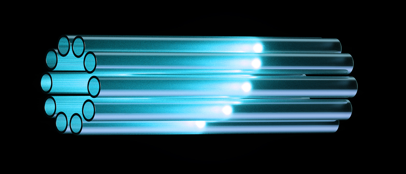
Figure 1: A gyrating soliton in the necklace of $2N=10$ waveguides (schematic representation).

There are several types of gyrating solitons coexisting in the array of the same number of guides. Some of these objects consist of a single pulse that spirals around the necklace; other ones comprise series of pulses of varied brightness. There are solitons with different propagation constants within each of the two varieties. While the systematic classification of stability properties of the gyrating solitons is beyond the scope of the present study, our analysis indicates that some of these are stable.

The paper is organised as follows. In the next section (section II) we classify linear supermodes in the nondispersive necklace. These will serve as starting points for the bifurcating nonlinear patterns (section III). In section IV we consider constellations of pulses appearing simultaneously in all $2N$ waveguides and in sections V and VI discuss solitons oscillating between even and odd subsets of the array. Solitons whose motion along the fiber is accompanied by their gyration around the necklace, are introduced in section VII. In the subsequent section (VIII) we consider more complex, multiflash, gyrating patterns. Stability and interaction of gyrating solitons are touched upon in section IX. Section X summarises results of this study.

II Linear nondispersive waveguides

The necklace of waveguides is described by the following system of $2N$ equations written in the reference frame traveling at the common group velocity Mumtaz ; Chekh :

$$i\partial_{z}\psi_{n}+\partial_{\tau}^{2}\psi_{n}+\psi_{n-1}+\psi_{n+1}+2|\psi_{n}|^{2}\psi_{n}=2i\Gamma_{n}\psi_{n}.$$ (1)

Here $\psi_{n}$ is the amplitude of the complex mode in the $n$-th core ($n=1,...,2N$); $z$ measures length along the device and $\tau$ is a retarded time. We are considering waveguides with an anomalous group velocity dispersion and all coefficients have been normalised to unity.

In the system (1) we have assumed that waveguides with gain and loss alternate:

$$\Gamma_{n}=(-1)^{n+1}\gamma.$$

Here $\gamma>0$ is a common gain-loss coefficient. Skipping ahead a bit, many of our results will remain valid for the hermitian array, $\gamma=0$.

The equation (1) with $n=1$ contains an unknown $\psi_{0}$ and the equation with $n=2N$ includes $\psi_{2N+1}$. These two variables are defined by virtue of the periodicity condition:

$$\psi_{n+2N}=\psi_{n}.$$

We start by examining the linear nondispersive limit of (1) which results from dropping the nonlinearity and time derivative $\partial_{\tau}^{2}\psi_{n}$. Assuming a separable solution of the form $\psi_{n}=v_{n}e^{i\beta z}$, the coefficients $v_{n}$ comprise an eigenvector ${\vec{v}}=(v_{1},v_{2},...,v_{2N})^{T}$ of the matrix $\mathcal{L}$:

$$\mathcal{L}{\vec{v}}=\beta{\vec{v}},$$

where

$$\mathcal{L}_{nm}=\delta_{n,m-1}+\delta_{n,m+1}-2i\Gamma_{n}\delta_{n,m}.$$ (2)

The $\delta$-symbol in (2) is $2N$-periodic:

$$\delta_{n,m}=\left\{\begin{array}[]{ll}1,&n=m\ \mathrm{mod}(2N);\\ 0,&\mbox{otherwise}.\end{array}\right.$$

The eigenvalues of $\mathcal{L}$ were determined in Liam :

$$\beta=\pm\beta_{\alpha},\quad\beta_{\alpha}=2\sqrt{\cos^{2}\left(\frac{k_{\alpha}}{2}\right)-\gamma^{2}}>0,$$

$$k_{\alpha}=\frac{2\pi}{N}\alpha,\quad\alpha=1,2,...,N.$$ (3)

The eigenvalues are all real if $\gamma\leq\gamma_{c}$, where

$$\gamma_{c}(N)=\left\{\begin{array}[]{ll}0,&N=\mbox{even};\\ \sin\left(\frac{\pi}{2N}\right),&N=\mbox{odd}.\end{array}\right.$$ (4)

Note that in the necklace with even $N$, the eigenvalues become complex as soon as $\gamma$ is nonzero. For this reason we are only considering odd $N$ in what follows. We are also assuming that the symmetry is not broken, that is, $\gamma\leq\gamma_{c}$.

Two eigenvalues, $\beta_{N}$ and $-\beta_{N}$, are simple (non-repeated). The other $\frac{N-1}{2}$ positive and $\frac{N-1}{2}$ negative eigenvalues have algebraic multiplicity 2. Indeed, $\beta_{\alpha}$ coincides with $\beta_{(N-\alpha)}$ for all $\alpha=1,2,...N-1$.

Turning to the eigenvectors of $\mathcal{L}$, one can readily check that

$${\vec{v}}^{(\alpha)}=\left(e^{ik+i\theta},e^{ik},e^{2ik+i\theta},e^{2ik},...,e^{Nik+i\theta},e^{Nik}\right)^{T}$$ (5)

is an eigenvector corresponding to a positive eigenvalue $\beta=\beta_{\alpha}$. Here $k=k_{\alpha}$ is as in (3) and $\theta=\theta_{\alpha}$ is defined by

$$e^{i\theta_{\alpha}}=\frac{1+e^{-ik_{\alpha}}}{2i\gamma+\beta_{\alpha}},\quad\alpha=1,2,...N.$$

It is not difficult to verify that the vectors ${\vec{v}}^{(\alpha)}$ and ${\vec{v}}^{(N-\alpha)}$ are linearly independent for all $\alpha=1,2,...,\frac{N-1}{2}$ and so each positive eigenvalue $\beta=\beta_{\alpha}$ has a geometric multiplicity 2.

The vector

$${\vec{w}}^{(\alpha)}=\left(e^{ik+i\phi},e^{ik},e^{2ik+i\phi},e^{2ik},...,e^{Nik+i\phi},e^{Nik}\right)^{T},$$ (6)

where $k=k_{\alpha}$ is as in (3) and $\phi=\phi_{\alpha}$ is defined by

$$e^{i\phi_{\alpha}}=\frac{1+e^{-ik_{\alpha}}}{2i\gamma-\beta_{\alpha}},\quad\alpha=1,2,...N,$$

is an eigenvector associated with a negative eigenvalue $\beta=-\beta_{\alpha}$. Since the eigenvectors ${\vec{w}}^{(\alpha)}$ and ${\vec{w}}^{(N-\alpha)}$ pertaining to the equal eigenvalues $-\beta_{N-\alpha}$ and $-\beta_{\alpha}$ are linearly independent for any $1\leq\alpha\leq\frac{N-1}{2}$, we conclude that each repeated negative eigenvalue of the matrix $\mathcal{L}$ has a geometric multiplicity 2 as well.

III Nonlinear selection rule

Returning to the nonlinear dispersive system (1), we introduce a hierarchy of stretched coordinates $Z_{\ell}=\epsilon^{\ell}z$ and time scales $T_{\ell}=\epsilon^{\ell}\tau$; $\ell=0,1,2,...$. In the limit $\epsilon\to 0$ all these variables become independent and the chain rule gives

$$\frac{\partial}{\partial z}=D_{0}+\epsilon^{2}D_{2}+\epsilon^{4}D_{4}+...,\quad\frac{\partial}{\partial\tau}=\partial_{0}+\epsilon\partial_{1}+\epsilon^{2}\partial_{2}+...,$$

where $D_{\ell}=\partial/\partial Z_{\ell}$ and $\partial_{\ell}=\partial/\partial T_{\ell}$. Symmetry considerations suggest that the complex modes $\psi_{n}$ should not depend on the odd coordinates $Z_{1},Z_{3},...$, — this is why we have omitted the odd terms in the expansion of $\partial_{z}$. Expanding

$$\psi_{n}=\epsilon A_{n}+\epsilon^{3}B_{n}+...$$

and substituting into (1) we equate coefficients of like powers of $\epsilon$.

The order $\epsilon^{1}$ gives

$$iD_{0}{\vec{A}}+\mathcal{L}{\vec{A}}=0,$$ (7)

where ${\vec{A}}=(A_{1},A_{2},...,A_{2N})^{T}$ and we have assumed that $\vec{A}$ does not change on the fast time scale, $T_{0}$. The general solution of (7) is given by a linear combination

$${\vec{A}}=\sum_{\alpha=1}^{N}p^{(\alpha)}{\vec{v}}^{(\alpha)}e^{i\beta_{\alpha}z}+\sum_{\alpha=1}^{N}r^{(\alpha)}{\vec{w}}^{(\alpha)}e^{-i\beta_{\alpha}z},$$ (8)

where the constant vectors ${\vec{v}}^{(\alpha)}$ and ${\vec{w}}^{(\alpha)}$ are as in (5) and (6) while the scalar coefficients $p^{(\alpha)}$ and $r^{(\alpha)}$ are assumed to depend on the “slow” variables $Z_{2},Z_{4},...$ and $T_{1},T_{2},...$. The individual terms in (8) are commonly referred to as supermodes. The sum (8) with a specific choice of coefficients will be called a “linear pattern” in what follows.

To determine nonlinear constraints that select particular linear patterns in the necklace, we proceed to the order $\epsilon^{3}$ which gives a nonhomogeneous system of equations for coefficients $B_{n}$:

$$iD_{0}{\vec{B}}+\mathcal{L}{\vec{B}}={\vec{\mathcal{R}}},$$ (9)

where

$${\mathcal{R}}_{n}=-\left(iD_{2}+\partial_{1}^{2}+2|A_{n}|^{2}\right)A_{n};$$

$n=1,2,...,2N$. The vector function ${\vec{\mathcal{R}}}$ will generally have terms that are in resonance with the “frequencies” of the linear nondispersive system. The unbounded growth of the coefficients $B_{n}$ as $z\to\infty$ (and the resulting breakdown of the asymptotic expansion) can only be avoided if ${\vec{\mathcal{R}}}$ is orthogonal to the eigenvectors of the matrix $\mathcal{L}$. These orthogonality relations: (a) select the linear patterns that persist in the nonlinear dispersive regime when the amplitudes of the complex modes are no longer small and the beams are no longer stationary; (b) determine the longitudinal structure and temporal evolution of nonlinear pulses of light.

In the subsequent sections we go over several possible choices in (8).

IV Simultaneous pulses in $2N$ guides

Circular-symmetric distributions of power $|\psi_{n}|^{2}$ result by keeping only one supermode in the linear pattern (8). Choosing

$${\vec{A}}=p{\vec{v}}^{(N)}e^{i\beta z},$$ (10)

where $\beta=\beta_{N}$ and $p=p^{(N)}$, a bounded solution to equations (9) (if exists) will have the form

$${\vec{B}}={\vec{\mathcal{X}}}e^{i\beta z},$$ (11)

where ${\vec{\mathcal{X}}}$ satisfies

$$(\mathcal{L}-\beta I)\vec{\mathcal{X}}=-(iD_{2}p+\partial_{1}^{2}p+2|p|^{2}p)\vec{v}^{(N)}.$$ (12)

The singular system (12) admits a solution if and only if its right-hand side is orthogonal to the eigenvector ${\vec{v}}^{(N)}$ in the sense of the dot product

$${\vec{y}}\cdot{\vec{z}}=\sum_{n=1}^{2N}y_{n}z_{n}.$$ (13)

[In equation (13), $\vec{y}$ and $\vec{z}$ are vectors with complex components.] Making use of the identity

$${\vec{v}}^{\,(\alpha)}\cdot{\vec{v}}^{\,(\alpha)}=(1+e^{i\theta_{N}})N\delta_{\alpha,N}$$ (14)

with $\alpha=N$, the solvability condition reduces to the nonlinear Schrödinger equation

$$i\frac{\partial p}{\partial Z_{2}}+\frac{\partial^{2}p}{\partial T_{1}^{2}}+2|p|^{2}p=0.$$ (15)

A localised solution of equation (15) is the soliton

$$p=e^{iZ_{2}}\mathrm{sech}\,T_{1},$$ (16)

where the amplitude has been set equal to 1. (There is no loss in generality in setting the amplitude to unity as it only appears as a coefficient in front of $\epsilon$ when the solution is expressed in the original coordinates.) The vector function (10) with $p$ as in (16) describes identical light pulses travelling in $2N$ waveguides level with each other. All waveguides shine in unison and with the same intensity: $|\psi_{n}|^{2}=\epsilon^{2}\mathrm{sech}^{2}(\epsilon\tau)$.

Another simultaneous ring of pulses results by letting $r^{(\alpha)}=0$ for all $\alpha=1,...,N$, and $p^{(\alpha)}=0$ for all $\alpha$ except one particular value $\alpha=\alpha_{0}$ and its symmetric partner $\alpha=N-\alpha_{0}$. Here $1\leq\alpha_{0}\leq\frac{N-1}{2}$. Denoting

$$p^{(\alpha_{0})}\equiv p,\quad p^{(N-\alpha_{0})}\equiv q,\quad{\vec{v}}^{(\alpha_{0})}\equiv{\vec{v}},\quad{\vec{v}}^{(N-\alpha_{0})}\equiv{\vec{u}},$$

and $\beta_{\alpha_{0}}=\beta$, the linearised pattern (8) becomes

$${\vec{A}}=\left(p{\vec{v}}+q{\vec{u}}\right)e^{i\beta z}.$$ (17)

A bounded third-order correction $B_{n}$ has the form (11), where the vector $\vec{\mathcal{X}}$ satisfies the system

$$\sum_{m=1}^{2N}\mathcal{L}_{nm}\mathcal{X}_{m}-\beta\mathcal{X}_{n}=-Fv_{n}-Gu_{n}$$

$$-2\left[q^{2}p^{*}u_{n}^{2}v_{n}^{*}+p^{2}q^{*}v_{n}^{2}u_{n}^{*}\right]$$ (18)

with the coefficient functions

$$F(Z_{2},...,T_{1},...)=\left(iD_{2}+\partial_{1}^{2}+2|p|^{2}+4|q|^{2}\right)p,$$ (19)

$$G(Z_{2},...,T_{1},...)=\left(iD_{2}+\partial_{1}^{2}+4|p|^{2}+2|q|^{2}\right)q.$$ (20)

Since the zero eigenvalue of the matrix $\mathcal{L}-\beta I$ in the left-hand side of (18) has geometric multiplicity 2, the nonhomogeneous system (18) has two solvability conditions. Taking the scalar product of its right-hand side with $\vec{u}$ and $\vec{v}$ produces a pair of amplitude equations:

$$i\frac{\partial p}{\partial Z_{2}}+\frac{\partial^{2}p}{\partial T_{1}^{2}}+2(|p|^{2}+2|q|^{2})p=0,$$ (21a)

$$i\frac{\partial q}{\partial Z_{2}}+\frac{\partial^{2}q}{\partial T_{1}^{2}}+2(|q|^{2}+2|p|^{2})q=0.$$ (21b)

In obtaining the system (21), we used the following two identities in addition to the identity (14):

$${\vec{v}}^{(\alpha)}\cdot{\vec{v}}^{(N-\alpha)}=\left(e^{i(k_{\alpha}+2\theta_{\alpha})}+1\right)N,$$ (22)

$$\sum_{n=1}^{2N}v_{n}^{3}u_{n}^{*}=\sum_{n=1}^{2N}u_{n}^{3}v_{n}^{*}=0.$$

The power distribution associated with a repeated eigenvalue $\beta_{\alpha_{0}}$ is $z$-independent but not uniform across the necklace. Letting, for simplicity, $p=q$, equation (17) gives

$$|A_{n}|^{2}=2|p|^{2}\left[1+\cos(nk_{\alpha_{0}})\right].$$

A localised pattern arises when the soliton solution of (21) is chosen:

$$p=q=\frac{1}{\sqrt{3}}e^{iZ_{2}}\mathrm{sech}\,T_{1}.$$ (23)

The vector (17) with $p$ and $q$ as in (23) describes a ring-shaped constellation of light pulses travelling abreast in $2N$ fibers. The pulse power undergoes a sinusoidal variation along the ring.

Earlier studies of simultaneous pulses in circular arrays of coupled hermitian waveguides were reported in Refs syncsol ; Akhmediev ; Liam . In Akhmediev , rings of solitonic pulses with varying power were described as bifurcations of the uniformly powered ring. Our perspective here is different; we have considered simultaneous pulses as nonlinear perturbations of nonuniform linear patterns.

V Uniform breathers

Keeping terms with both positive and negative propagation constants in the linear pattern (8) gives rise to $z$-dependent power distributions. The simplest possibility corresponds to retaining just two terms:

$${\vec{A}}=p{\vec{v}}e^{i\beta z}+q{\vec{w}}e^{-i\beta z}.$$ (24)

Here $\beta=\beta_{N}$ is a simple positive eigenvalue, while

$${\vec{v}}={\vec{v}}^{(N)},\quad{\vec{w}}={\vec{w}}^{(N)}$$

are the eigenvectors corresponding to $\beta_{N}$ and its negative, respectively. With this choice, the bounded solution of equation (9) is

$${\vec{B}}=\vec{\mathcal{X}}e^{i\beta z}+\vec{\mathcal{Y}}e^{-i\beta z}+\vec{\mathcal{M}}e^{3i\beta z}+\vec{\mathcal{N}}e^{-3i\beta z},$$ (25)

where the amplitudes $\vec{\mathcal{X}}$ and $\vec{\mathcal{Y}}$ satisfy nonhomogeneous algebraic equations with singular matrices:

$$\left(\mathcal{L}-\beta I\right)\vec{\mathcal{X}}=-F\vec{v},$$ (26)

$$\left(\mathcal{L}+\beta I\right)\vec{\mathcal{Y}}=-G\vec{w}.$$ (27)

Here $F$ and $G$ are as in (19) and (20).

Equation (26) admits a solution if and only if its right-hand side is orthogonal to ${\vec{v}}$ while the right-hand side of (27) should be orthogonal to ${\vec{w}}$. (Here orthogonality is understood in the sense of the dot product (13).) Using (14) and the identity

$${\vec{w}}^{\,(\alpha)}\cdot{\vec{w}}^{\,(\alpha)}=(1+e^{i\phi_{N}})N\delta_{\alpha,N}$$

with $\alpha=N$, these orthogonality constraints translate into equations (21).

Letting $q=p$, equation (24) gives rise to an oscillatory power distribution:

$$|A_{2m-1}|^{2}=4|p|^{2}\sin^{2}(\beta z+\theta_{N}),$$

$$|A_{2m}|^{2}=4|p|^{2}\cos^{2}(\beta z),$$

$m=1,2,...,N$. This describes a flashing necklace: all odd waveguides blink in unison and all even waveguides reach their maximum power at the same $z$, but there is a lag between the odd and even. Note that the flashing is uniform: the maximum power is the same for all waveguides.

The soliton solution (23) of the system (21) provides an envelope for a finite-duration sequence of short flashes in the necklace — a spatio-temporal pattern commonly referred to as a breather. Breathers in fiber directional couplers (that is, in necklaces consisting just of 2 waveguides, with no gain or loss) were described numerically and variationally coupler . For the asymptotic descriptions and nonhermitian extensions, see BSSDK .

VI Nonuniform flashing

A set of slightly more complex patterns results by letting, in equation (8), $r^{(\alpha)}=0$ and $p^{(\alpha)}=0$ for all $\alpha=1,2,...,N$ except one particular value $\alpha=\alpha_{0}$ ($1\leq\alpha_{0}\leq\frac{N-1}{2}$) and its symmetric partner $\alpha=N-\alpha_{0}$. Denoting

$$p^{(\alpha_{0})}\equiv p_{1},\ r^{(\alpha_{0})}\equiv q_{1},\ r^{(N-\alpha_{0})}\equiv p_{2},\ p^{(N-\alpha_{0})}\equiv q_{2}$$

and $\beta_{\alpha_{0}}=\beta$, equation (8) becomes

$${\vec{A}}={\vec{\eta}}e^{i\beta z}+{\vec{\xi}}e^{-i\beta z}$$ (28a)

where

$${\vec{\eta}}=p_{1}{\vec{v}}^{(\alpha_{0})}+q_{2}{\vec{v}}^{(N-\alpha_{0})},\ {\vec{\xi}}=q_{1}{\vec{w}}^{(\alpha_{0})}+p_{2}{\vec{w}}^{(N-\alpha_{0})}.$$ (28b)

The next-order correction has the form (25) where $\vec{\mathcal{X}}$ and $\vec{\mathcal{Y}}$ satisfy

$$(\mathcal{L}-\beta I){\vec{\mathcal{X}}}=-{\vec{\mathcal{F}}},$$ (29)

$$(\mathcal{L}+\beta I){\vec{\mathcal{Y}}}=-{\vec{\mathcal{G}}},$$ (30)

with

$$\mathcal{F}_{n}=iD_{2}\eta_{n}+\partial_{1}^{2}\eta_{n}+2(|\eta_{n}|^{2}+2|\xi_{n}|^{2})\eta_{n},$$

$$\mathcal{G}_{n}=iD_{2}\xi_{n}+\partial_{1}^{2}\xi_{n}+2(2|\eta_{n}|^{2}+|\xi_{n}|^{2})\xi_{n}.$$

The zero eigenvalue of the matrix $\mathcal{L}-\beta I$ in equation (29) has geometric multiplicity 2, and the same is true for the zero eigenvalue of the matrix $\mathcal{L}+\beta I$ in (30). Evaluating the dot product of the right-hand side of (29) with the vectors ${\vec{v}}^{(\alpha_{0})}$ and ${\vec{v}}^{(N-\alpha_{0})}$, and then taking the product of the right-hand side of (30) with ${\vec{w}}^{(\alpha_{0})}$ and ${\vec{w}}^{(N-\alpha_{0})}$, we arrive at a system of four amplitude equations:

$$i\frac{\partial p_{\mu}}{\partial Z_{2}}+\frac{\partial^{2}p_{\mu}}{\partial T_{1}^{2}}+2\left(|p_{\mu}|^{2}+2|p_{\mu+1}|^{2}\right)p_{\mu}$$

$$+4\left(|q_{1}|^{2}+|q_{2}|^{2}\right)p_{\mu}+4q_{1}q_{2}p_{\mu+1}^{*}=0,$$ (31a)

$$i\frac{\partial q_{\mu}}{\partial Z_{2}}+\frac{\partial^{2}q_{\mu}}{\partial T_{1}^{2}}+2\left(|q_{\mu}|^{2}+2|q_{\mu+1}|^{2}\right)q_{\mu}$$

$$+4\left(|p_{1}|^{2}+|p_{2}|^{2}\right)q_{\mu}+4p_{1}p_{2}q_{\mu+1}^{*}=0,$$ (31b)

where $\mu=1,2$. In (31), we use the cyclic notation for the indices: $p_{3}$ should be understood as $p_{1}$ and $q_{3}$ as $q_{1}$.

The system (31) is invariant under a 3-parameter transformation

$$q_{\mu}\to e^{i\varphi_{\mu}}q_{\mu},\quad p_{\mu}\to e^{i\vartheta_{\mu}}p_{\mu},\quad(\mu=1,2),$$ (32a)

where $$\varphi_{1,2} \vartheta_{1,2}$$ and are four constant angles satisfying

$$\varphi_{1}+\varphi_{2}=\vartheta_{1}+\vartheta_{2}.$$ (32b)

Solutions that are related by the transformation (32) will be regarded equivalent.

It is convenient to introduce vector notation for the four-component columns:

$$\mathbf{\Phi}=\left(\begin{array}[]{r}p_{1}\\ p_{2}\\ q_{1}\\ q_{2}\end{array}\right).$$

There are ${\textstyle\left(\begin{array}[]{c}4\\ 2\end{array}\right)}=6$ nonequivalent soliton solutions with two nonzero components:

$$\mathbf{\Phi}^{(12)}=\left(\begin{array}[]{r}1\\ 0\\ 0\\ 1\end{array}\right)f,\quad\mathbf{\Phi}^{(21)}=\left(\begin{array}[]{r}0\\ 1\\ 1\\ 0\end{array}\right)f,\quad\mathbf{\Phi}^{(11)}=\left(\begin{array}[]{r}1\\ 0\\ 1\\ 0\end{array}\right)f,$$

$$\mathbf{\Phi}^{(22)}=\left(\begin{array}[]{r}0\\ 1\\ 0\\ 1\end{array}\right)f,\quad\mathbf{\Phi}^{(p)}=\left(\begin{array}[]{r}1\\ 1\\ 0\\ 0\end{array}\right)f,\quad\mathbf{\Phi}^{(q)}=\left(\begin{array}[]{r}0\\ 0\\ 1\\ 1\end{array}\right)f,$$

where $f$ accounts for the large-scale space-time variation of the pattern:

$$f(Z_{2},T_{1})=\frac{1}{\sqrt{3}}e^{iZ_{2}}\mathrm{sech}\,T_{1}.$$ (33)

The solution $\mathbf{\Phi}^{(12)}$ reproduces equation (17) with $p$ and $q$ as in (23). This solution as well as $\mathbf{\Phi}^{(21)}$ describe constellations of $2N$ pulses travelling abreast, with their power varying along the necklace. On the other hand, $\mathbf{\Phi}^{(11)}$ and $\mathbf{\Phi}^{(22)}$ define uniformly flashing patterns similar to (24).

Deferring the intepretation of $\mathbf{\Phi}^{(p)}$ and $\mathbf{\Phi}^{(q)}$ to the next section, here we consider two more soliton solutions of the system (31). Both solutions have all their components nonzero:

$$\mathbf{\Phi}^{(A)}=\frac{1}{\sqrt{3}}\left(\begin{array}[]{r}1\\ 1\\ 1\\ 1\end{array}\right)f,\quad\mathbf{\Phi}^{(B)}=\sqrt{\frac{3}{5}}\left(\begin{array}[]{r}1\\ 1\\ 1\\ -1\end{array}\right)f,$$ (34)

where $f(Z_{2},T_{1})$ is as in (33).

The power load of individual waveguides associated with the solution $\mathbf{\Phi}^{(A)}$ is given by

$$|A_{2m-1}|^{2}=\frac{16}{3}|f|^{2}\cos^{2}\left(\frac{2m-1}{2}k\right)$$

$$\times\sin^{2}\left(\beta z+\theta+\frac{k}{2}\right),$$

$$|A_{2m}|^{2}=\frac{16}{3}|f|^{2}\cos^{2}(mk)\cos^{2}(\beta z),$$ (35)

while the soliton $\mathbf{\Phi}^{(B)}$ carries the following power distribution:

$$|A_{2m-1}|^{2}=\frac{12}{5}|f|^{2}+\frac{12}{5}|f|^{2}\sin\left[(2m-1)k\right]$$

$$\times\sin(2\beta z+2\theta+k),$$

$$|A_{2m}|^{2}=\frac{12}{5}|f|^{2}-\frac{12}{5}|f|^{2}\sin(2mk)\sin(2\beta z).$$ (36)

In either of these equations, $m=1,2,...N$, and $\beta=\beta_{\alpha_{0}}$, $k=k_{\alpha_{0}}$, $\theta=\theta_{\alpha_{0}}$. Both (35) and (36) represent flashing patterns, or breathers, where all odd and all even waveguides flash synchronously. The maximum power attainable in an individual waveguide undergoes a sinusoidal variation along the necklace.

VII Gyrating solitons

VII.1 Single-frequency pattern

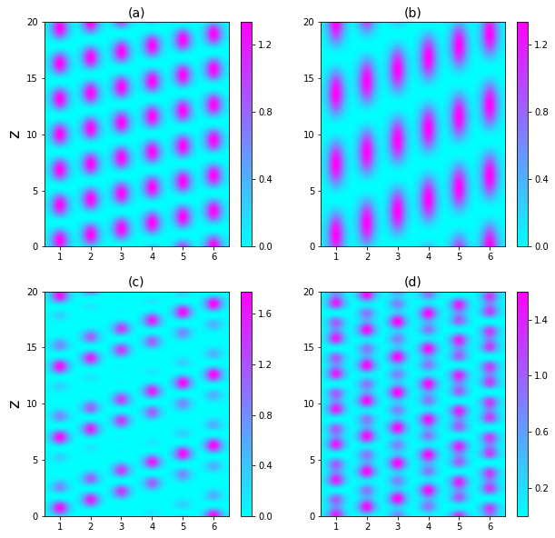
Figure 2: Four types of gyrating solitons in a necklace of $2N=6$ waveguides. Each panel consists of six vertical lanes displaying the $(\tau,z)$-distribution of optical power in six waveguides. The horizontal side of each lane represents a short period of time, $-20<\tau<20$; the $\tau$-axis is not marked or labelled. The vertical coordinate measures the length along the waveguides, with $0\leq z\leq 20$. (a) jiver soliton (41). The panel shows the power distribution (37). (b) the power density (43) corresponding to the waltzer (44). (c): power distribution (45) associated with the multiflash gyrator $A$. (d): power pattern (46) of the multiflash solution $B$. In all panels, $\gamma=0$ and $\alpha=1$. All solitons have the inverse-width parameter $\epsilon=0.1$.

The solitons $\mathbf{\Phi}^{(p)}$ and $\mathbf{\Phi}^{(q)}$ represent light pulses gyrating around the necklace.

The power distribution associated with $\mathbf{\Phi}^{(p)}$ has the form of a spiral wave (Fig 2(a)):

$$|A_{2m-1}|^{2}=4|f|^{2}\sin^{2}(km+\beta z+\theta),$$

$$|A_{2m}|^{2}=4|f|^{2}\cos^{2}(km+\beta z).$$ (37)

Here $m=1,2,...N$ and the parameters are $k=k_{\alpha}$, $\beta=\beta_{\alpha}$ and $\theta=\theta_{\alpha}$. To simplify the notation, we have dropped the subscript 0 from the index $\alpha$ ($1\leq\alpha\leq\frac{N-1}{2}$).

To establish whether the soliton is gyrating clockwise or counter-clockwise, we need to determine which of the two neighbours of the $2m$-th waveguide will flash immediately after the $2m$-th guide has. Assume that the $2m$-th waveguide attains its maximum power at the point $z=z_{0}$. Then the closest maximum of $|A_{2m+1}|^{2}$ to the right of $z_{0}$ is at $z=z_{0}+\Delta_{2m+1}$, and the nearest maximum of $|A_{2m-1}|^{2}$ to the right of $z_{0}$ is at $z=z_{0}+\Delta_{2m-1}$, where the delay intervals are given by

$$\Delta_{2m+1}=\frac{1}{\beta}\left(\frac{\pi}{2}-\theta-k\right)$$ (38)

and

$$\Delta_{2m-1}=\left\{\begin{array}[]{rc}-\frac{1}{\beta}\left(\frac{\pi}{2}+\theta\right)&\mbox{if}\ \theta<-\frac{\pi}{2},\\ \frac{1}{\beta}\left(\frac{\pi}{2}-\theta\right)&\mbox{if}\ \theta>-\frac{\pi}{2}.\end{array}\right.$$ (39)

Comparing the lags (38) and (39) one can readily check that the $(2m+1)$-th guide flashes sooner respectively later than the $(2m-1)$-th one if $\gamma<\gamma_{\alpha}$ respectively $\gamma>\gamma_{\alpha}$, where

$$\gamma_{\alpha}=\cos^{2}\frac{k_{\alpha}}{2}.$$

Let

$$\alpha_{c}(N)=\mathrm{floor}\left[\frac{N}{\pi}\arccos\left(\gamma_{c}^{1/2}\right)\right],$$ (40)

where $\mathrm{floor}[x]$ stands for the greatest integer less than or equal to $x$, while $\gamma_{c}=\sin\left(\frac{\pi}{2N}\right)$ is the linear $\mathcal{PT}$-symmetry breaking threshold given by equation (4). For all $\alpha\leq\alpha_{c}$ we have $\gamma_{\alpha}\geq\gamma_{c}$. Since we are considering a necklace operating in the stable regime $(\gamma<\gamma_{c})$, then, assuming that the waveguides are numbered against the clock, we conclude that the soliton $\mathbf{\Phi}^{(p)}$ with any $\alpha=1,2,...,\alpha_{c}$ and regardless of $\gamma$, is gyrating counterclockwise.

By contrast, the sense of gyration of the soliton $\mathbf{\Phi}^{(p)}$ with $\alpha=\alpha_{c}+1,...,\frac{N-1}{2}$ does depend on $\gamma$. The corresponding transition values $\gamma_{\alpha}$ lie under the $\mathcal{PT}$-symmetry breaking threshold. When $0\leq\gamma<\gamma_{\alpha}$, the soliton gyrates counterclockwise but when $\gamma_{\alpha}<\gamma<\gamma_{c}$, it revolves in the clockwise direction. This crossover is illustrated by Fig 3.

The behaviour of the solitons $\mathbf{\Phi}^{(q)}$ is opposite to that of $\mathbf{\Phi}^{(p)}$. Namely, pulses with $\alpha=1,2,...,\alpha_{c}$ are gyrating clockwise for all $\gamma$. Those with $\alpha=\alpha_{c}+1,...,\frac{N-1}{2}$ are also revolving clockwise for small $\gamma$ but their direction of gyration can be reversed by raising $\gamma$ above $\gamma_{\alpha}$.

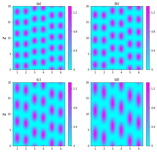
Figure 3: The transition from counterclockwise to clockwise gyration in the necklace of 6 waveguides. All four panels pertain to the same jiver soliton as in Fig 2(a) but with different $\gamma$. As in Fig 2, each panel consists of 6 vertical lanes. The $n$-th lane shows $|A_{n}(\tau,z)|^{2}$, the power density in the $n$-th waveguide. The horizontal side of each lane represents a short period of time, $-20<\tau<20$, with the $\tau$-axis not marked or labelled. The vertical coordinate measures the length along the waveguides. All four power distributions are given by equation (37) where $\alpha=1$, $\epsilon=0.1$ while $\gamma$ varies: (a) $\gamma=0.20$; (b) $\gamma=0.30$; (c) $\gamma=0.40$; (d) $\gamma=0.45$. The transition occurs as $\gamma$ is raised through $\gamma_{1}=0.25$.

The two gyrating solitons whose linear patterns are given by equation (28) with the coefficients defined by the vector $\mathbf{\Phi}^{(p)}$ or $\mathbf{\Phi}^{(q)}$, can be written in a unified way as

$${\vec{\psi}}=\epsilon\frac{{\vec{v}}^{(\alpha)}e^{i\beta_{\alpha}z}+{\vec{w}}^{(N-\alpha)}e^{-i\beta_{\alpha}z}}{\sqrt{3}}e^{i\epsilon^{2}z}\mathrm{sech}(\epsilon\tau)+O(\epsilon^{3}),$$ (41)

where $1\leq\alpha\leq N-1$. Solitons with $\alpha=N-\alpha_{c},...,N-1$ are gyrating clockwise and those with $\alpha=1,...,\alpha_{c}$ are moving against the clock. For $\alpha=\alpha_{c}+1,...,N-\alpha_{c}-1$, the direction of gyration is controlled by the choice of $\gamma$.

Before turning to other types of gyrating pulses we note two more characteristics of the solitons (41) that can be controlled in the nonhermitian situation. Namely, by varying the gain-loss coefficient one can change the length of the pulse and its period of revolution around the necklace. Both of these quantities are given by the $z$-period of the power density (37). The length of two particular pulses with $\alpha=\frac{N\pm 1}{2}$ can even be sent to infinity — one just needs to tune $\gamma$ to $\gamma_{c}$. (The reason is that the propagation constant $\beta_{(N\pm 1)/2}\to 0$ as $\gamma\to\gamma_{c}$.)

Fig 3 exemplifies the change in flash duration with a sequence of four values of $\gamma$ from the interval $(0,\gamma_{c})$.

VII.2 Two-frequency pattern

A quasiperiodic pattern that does not fit into the general Ansatz (28) combines eigenvectors associated with a repeated and a single eigenvalue:

$$\vec{A}=p{\vec{v}}^{(\alpha)}e^{i\beta_{\alpha}z}+q{\vec{v}}^{(N)}e^{i\beta_{N}z}.$$ (42)

Here $\alpha$ is an arbitrarily chosen mode number, $1\leq\alpha\leq N-1$. With this choice, the right-hand side of equation (9) features two resonant terms proportional to $e^{i\beta_{\alpha}z}$ and $e^{i\beta_{N}z}$, respectively. Since $\beta_{\alpha}$ is a repeated eigenvalue, the former term imposes two solvability conditions. With the help of (14), we verify that one of these is trivially satisfied. The other solvability condition, together with the solvability constraint associated with the propagation constant $\beta_{N}$, comprise the system (21). (The derivation makes use of the identities (14) and (22).)

Like the distribution (37) before, the power density associated with the pattern (42) has the form of a spiral:

$$|A_{2m-1}|^{2}=4|p|^{2}\cos^{2}\left[\frac{k_{\alpha}m+(\beta_{\alpha}-\beta_{N})z+\theta_{\alpha}-\theta_{N}}{2}\right],$$

$$|A_{2m}|^{2}=4|p|^{2}\cos^{2}\left[\frac{k_{\alpha}m+(\beta_{\alpha}-\beta_{N})z}{2}\right],$$ (43)

where $m=1,2,...,N$ and we have assumed a simple reduction of the system (21): $p=q$. (See Fig 2 (b).) A localised pattern corresponds to the soliton solution of that system, equation (23).

The self-contained form of the solution whose linear order is given by equation (42) with $p$ and $q$ as in (23), is

$${\vec{\psi}}=\epsilon\frac{{\vec{v}}^{(\alpha)}e^{i\beta_{\alpha}z}+{\vec{v}}^{(N)}e^{i\beta_{N}z}}{\sqrt{3}}e^{i\epsilon^{2}z}\mathrm{sech}(\epsilon\tau)+O(\epsilon^{3}).$$ (44)

This is a new gyrating soliton in the necklace. An argument similar to the one in section VII.1 shows that the solitons with $\alpha\geq\frac{N+1}{2}$ are gyrating clockwise while those with $\alpha\leq\frac{N-1}{2}$ are moving against the clock.

The panels (a) and (b) of Fig 2 illustrate the difference between the two types of gyrating solitons in the hermitian necklace of $6$ waveguides. The spiral pattern (43) displays a longer period of revolution around the necklace than the pattern (37). By the time the soliton (44) completes just one round of its “waltz” around the necklace, its more agile counterpart (41) will have “jived” around twice. For ease of reference, we dub the gyrating solitons (41) and (44) the jiver and the waltzer, respectively.

VIII Multiflash gyration

When the waveguides are linear and nondispersive, that is, when the necklace is described by the system (1) with neither cubic nor time-derivative terms included, any set of coefficients $p^{(\alpha)}$ and $r^{(\alpha)}$ in (8) defines a pattern in the necklace. However, only a handful of those patterns persist the addition of nonlinear and dispersive terms to (8).

In this section we identify two more spiral patterns associated with gyrating solitons. The patterns in question generalise the two-mode combination (42). They involve an eigenvector ${\vec{v}}^{(\alpha)}$ associated with a repeated eigenvalue $\beta_{\alpha}$ (where $1\leq\alpha\leq N-1$), its mirror-reflected conterpart ${\vec{w}}^{(N-\alpha)}$ associated with the negative propagation constant $-\beta_{\alpha}$, and the eigenvectors ${\vec{v}}^{(N)},{\vec{w}}^{(N)}$ corresponding to the pair of single eigenvalues $\pm\beta_{N}$:

$${\vec{A}}=p_{1}{\vec{v}}^{(\alpha)}e^{i\beta_{\alpha}z}+p_{2}{\vec{w}}^{(N-\alpha)}e^{-i\beta_{\alpha}z}$$

$$+q_{1}{\vec{v}}^{(N)}e^{i\beta_{N}z}+q_{2}{\vec{w}}^{(N)}e^{-i\beta_{N}z}.$$

This time, the right-hand side of equation (9) has four resonant terms proportional to $e^{\pm i\beta_{\alpha}z}$ and $e^{\pm i\beta_{N}z}$. Two of the six solvability conditions are satisfied automatically while the remaining four amount to the system (31).

Two nonequivalent solutions of the system (31) with all components nonzero are given by equations (34). The power distribution associated with the solution $\mathbf{\Phi}^{(A)}$ has the form

$$|A_{2m-1}|^{2}=\frac{4}{3}|f|^{2}\left[\sin(\beta_{N}z+\theta_{N})\right.$$

$$\left.+\sin(mk_{\alpha}+\beta_{\alpha}z+\theta_{\alpha})\right]^{2},$$

$$|A_{2m}|^{2}=\frac{4}{3}|f|^{2}\left[\cos(\beta_{N}z)+\cos(mk_{\alpha}+\beta_{\alpha}z)\right]^{2}.$$ (45)

Here $m=1,2,...N$ and the slowly changing amplitude $f$ is given by (33). The power distribution (45) describes several flashes of unequal brightness appearing in rapid succession. The string of pulses gyrates around the necklace as a whole, with the ordering of bright and dim flashes changing from one waveguide to another.

Fig 2(c) illustrates a multiflash string (45) in a necklace of $2N=6$ guides. In this case the string comprises a bright flash and one or two dim pulses appearing short distances apart. In waveguides on one side of the necklace, the bright flash comes before the dim signal and on the other side the bright pulse follows the dim one.

The power distribution corresponding to the solution $\mathbf{\Phi}^{(B)}$ is

$$|A_{2m-1}|^{2}=\frac{12}{5}|f|^{2}\left[\cos^{2}(\beta_{N}z+\theta_{N})\right.$$

$$\left.+\sin^{2}(mk_{\alpha}+\beta_{\alpha}z+\theta_{\alpha})\right],$$

$$|A_{2m}|^{2}=\frac{12}{5}|f|^{2}\left[\sin^{2}(\beta_{N}z)+\cos^{2}(mk_{\alpha}+\beta_{\alpha}z)\right].$$ (46)

Here $m=1,2,...N$ and the coefficient function $f$ is as in (33). As the power pattern (45), the distribution (46) describes a multiflash string gyrating around the necklace (see Fig 2(d)).

Although the multiflash patterns have more complex power distributions than the spirals (37) and (43), they play an important role in the dynamics of the necklace. Numerical simulations indicate that the multiflash gyrating strings may emerge as products of the evolution of the unstable single-pulse gyrators (37). (See section IX.1 below.)

For future reference, we reproduce the multiflash gyrating solitons in a self-contained form:

$${\vec{\psi}}_{A}=\epsilon\left({\vec{v}}^{(\alpha)}e^{i\beta_{\alpha}z}+{\vec{w}}^{(N-\alpha)}e^{-i\beta_{\alpha}z}+{\vec{v}}^{(N)}e^{i\beta_{N}z}\right.$$

$$\left.+{\vec{w}}^{(N)}e^{-i\beta_{N}z}\right)\frac{e^{i\epsilon^{2}z}}{3}\mathrm{sech}(\epsilon\tau)+O(\epsilon^{3});$$ (47)

$${\vec{\psi}}_{B}=\epsilon\left({\vec{v}}^{(\alpha)}e^{i\beta_{\alpha}z}+{\vec{w}}^{(N-\alpha)}e^{-i\beta_{\alpha}z}+{\vec{v}}^{(N)}e^{i\beta_{N}z}\right.$$

$$\left.-{\vec{w}}^{(N)}e^{-i\beta_{N}z}\right)\frac{e^{i\epsilon^{2}z}}{\sqrt{5}}\mathrm{sech}(\epsilon\tau)+O(\epsilon^{3}).$$ (48)

As the notation suggests, we call (47) and (48) the $A$- and $B$-multiflash gyrator, respectively.

IX Soliton dynamics

IX.1 Stability and scattering of gyrating solitons

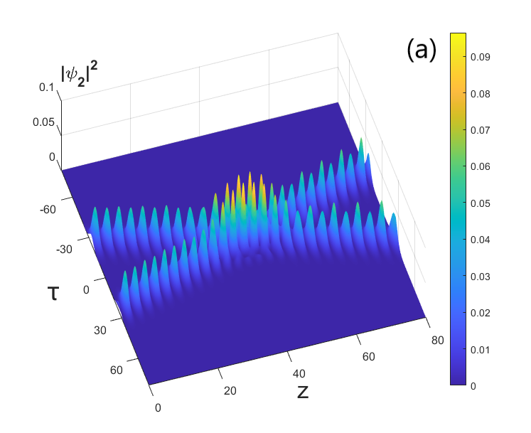
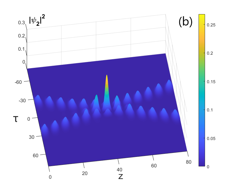
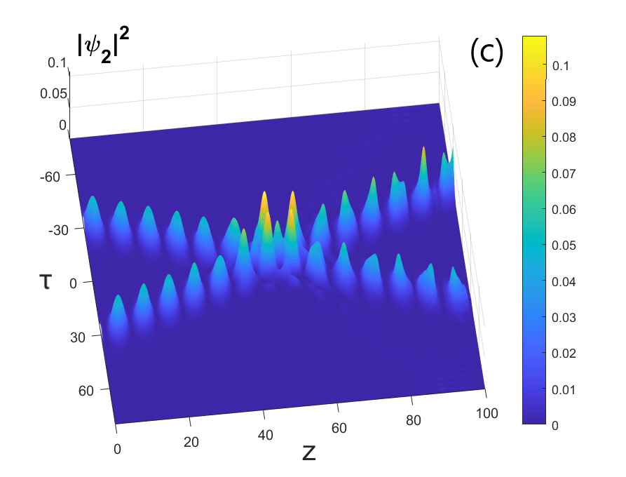
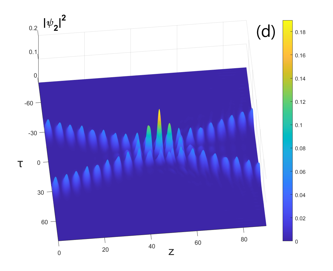
Figure 4: Scattering of gyrating solitons in the necklace of $2N=6$ waveguides. Shown is $|\psi_{2}|^{2}$, the power density in the second waveguide. (a,c) Collision of two “jiving” solitons with opposite sense of gyration. The initial condition is (50) with $\alpha=1$, $\epsilon=0.2$, and $V=0.6$. Panel (a) corresponds to $\gamma=0$ and panel (c) to $\gamma=0.45$. In either case, the products of collision constitute solitons with the modulated flashing amplitude. (The modulation is manifested in the alternation of peaks of unequal height.) (b,d) Collision of two waltzers. The initial condition is (IX.1) with $\alpha=1$, $\epsilon=0.2$, and $V=0.6$. Panels (b) and (d) depict the scattering process in the system (1) with $\gamma=0$ and $\gamma=0.45$, respectively. In both cases the post-collision solitons restore their original shape.

The comprehensive stability analysis of gyrating solitons is beyond the scope of the present study. Here, we restrict ourselves to a few sets of numerical simulations verifying that these novel objects do not blow up, disperse or transmute into non-gyrating localised structures within a short period of time.

All our computer simulations were carried out on the necklace of six waveguides ($N=3$). We considered the system (1) both in the hermitian ($\gamma=0$) and $\mathcal{PT}$-symmetric ($\gamma\neq 0$) situation.

Our first series of simulations involved the “jiving” soliton, equation (41) with $\alpha=1$ (Fig 2 (a)). The jiver was found to be weakly unstable, both for $\gamma=0$ and $\gamma\neq 0$. Choosing the initial condition in the form (41) with $\epsilon=0.1$ or $\epsilon=0.2$, and neglecting the $O(\epsilon^{3}$) terms, the resulting oscillatory solution was seen to slowly evolve into the multiflash solution (47). The pattern shown in Fig 2 (a) would gradually transform into the density profile of Fig 2 (c).

By contrast, the “waltzing” soliton in the same system has turned up to be stable for all values of $\gamma$ that we examined, including $\gamma=0$. Random noise added to the initial condition in the form (44) with $\alpha=1$ and $\epsilon=0.1$ or $0.2$, did not produce any measurable growth of the perturbation. The pattern shown in Fig 2 (b) would remain visibly unchanged.

It is instructive to compare the interaction of two jivers to the scattering of two waltzing solitons. We note that the system (1) has the Galilei invariance; namely, if $\psi_{n}(\tau,z)$ is a solution, then so is

$${\tilde{\psi}}_{n}(\tau,z)\equiv e^{i\frac{V}{2}\left(\tau-\frac{V}{2}z\right)}\psi_{n}(\tau-Vz,z).$$

In particular, if $\psi$ is a quiescent, unmoving, soliton, then ${\tilde{\psi}}$ gives the pulse travelling with the velocity $V$.

Making use of the Galilei transformation we set up an initial condition for the collision of two clockwise-gyrating jivers with equal amplitudes and equal oppositely-directed velocities:

$$\psi_{n} =\frac{\epsilon}{\sqrt{3}}\left(v_{n}^{(\alpha)}+w_{n}^{(N-\alpha)}\right)\left\{e^{i\frac{V}{2}\tau}\mathrm{sech}\left[\epsilon(\tau+\tau_{0})\right]\right.$$

$$+\left.e^{-i\frac{V}{2}\tau}\mathrm{sech}\left[\epsilon(\tau-\tau_{0})\right]\right\};\quad n=1,...,2N.$$ (49)

The collision of a clockwise and anti-clockwise jiving solitons was simulated using an initial condition of the form

$$\psi_{n} =\frac{\epsilon}{\sqrt{3}}\left\{\left(v_{n}^{(\alpha)}+w_{n}^{(N-\alpha)}\right)e^{i\frac{V}{2}\tau}\mathrm{sech}[\epsilon(\tau+\tau_{0})]\right.$$

$$+\left.\left(v_{n}^{(N-\alpha)}+w_{n}^{(\alpha)}\right)e^{-i\frac{V}{2}\tau}\mathrm{sech}[\epsilon(\tau-\tau_{0})]\right\},$$ (50)

where $n=1,...,2N$.

Despite the jiver’s weak instability, both the co-gyrating and counter-gyrating soliton pair emerged from the collision unscathed. In the case of either initial condition, equation (49) or (50), the only effect of interaction was an acquired modulation of each soliton’s oscillation amplitude (Fig 4(a,c)).

Turning to the collision of two waltzers, we set the initial condition in the form

$${\vec{\psi}}=\frac{\epsilon}{\sqrt{3}}({\vec{v}}^{(\alpha)}+{\vec{v}}^{(N)})\left\{e^{i\frac{V}{2}\tau}\mathrm{sech}\left[\epsilon(\tau+\tau_{0})\right]\right.$$

$$+\left.e^{-i\frac{V}{2}\tau}\mathrm{sech}\left[\epsilon(\tau-\tau_{0})\right]\right\}.$$ (51)

In this case, the scattering was seen to be elastic. The solitons would emerge without any change in the amplitude, velocity or the gyrating pattern (Fig 4 (b,d)).

IX.2 Vector Schrödinger equations

The two-component amplitude equation (21) and its four-component counterpart (31) are worth commenting upon.

The vector nonlinear Schrödinger equation (21) appeared in a large number of contexts and significant wealth of knowledge about its solutions has been accumulated 2NLS ; MT ; multihump ; BSSDK . Specifically, the soliton (23) was proved to be stable MT ; BSSDK and localised solutions with an arbitrary number of humps were determined in addition to this fundamental soliton multihump . By contrast, the four-component Schrödinger equation (31) is not in the existing literature.

An interesting property of equations (21) and (31) is their conservativity. In particular, equation (31) represents a Hamiltonian system with the Hamilton function

$$H=\int\left[|\dot{p}_{1}|^{2}+|\dot{p}_{2}|^{2}+|\dot{q}_{1}|^{2}+|\dot{q}_{2}|^{2}\phantom{|^{\frac{1}{2}}}\right.$$

$$+|p_{1}|^{4}+|p_{2}|^{4}+|q_{1}|^{4}+|q_{2}|^{4}\phantom{|^{\frac{1}{2}}}$$

$$-2\left(|p_{1}|^{2}+|p_{2}|^{2}+|q_{1}|^{2}+|q_{2}|^{2}\right)^{2}\phantom{|^{\frac{1}{2}}}$$

$$\left.\phantom{|^{\frac{1}{2}}}-4(p_{1}p_{2}q_{1}^{*}q_{2}^{*}+p_{1}^{*}p_{2}^{*}q_{1}q_{2})\right]dT_{1},\phantom{|^{\frac{1}{2}}}$$

where the overdot stands for $\partial/\partial T_{1}$. Equations (31) can be written as

$$i\frac{\partial p_{n}}{\partial Z_{2}}=\frac{\delta H}{\delta p_{n}^{*}},\quad i\frac{\partial q_{n}}{\partial Z_{2}}=\frac{\delta H}{\delta q_{n}^{*}}\quad(n=1,2),$$

where $p_{1,2}^{*}$ are the momenta canonically conjugate to the coordinates $p_{1,2}$, and $q_{1,2}^{*}$ are the momenta conjugate to $q_{1,2}$.

Thus, despite the presence of gain and loss, the small-amplitude light pulses in the $\mathcal{PT}$-symmetric necklace obey Hamiltonian dynamics.

X Concluding remarks

X.1 Conclusions

When the coupled waveguides considered in this paper are linear and non-dispersive — that is, when the system is modelled by the linear chain of $2N$ elements — the complex modes are given by arbitrary linear combinations of eigenvectors of the $2N\times 2N$ matrix (2). The addition of the nonlinearity and dispersion imposes nonlinear constraints on the coefficients of the admissible combinations. We have classified linear patterns that persist in the nonlinear dispersive necklace.

One simple pattern arising in the necklace of $2N$ linear waveguides corresponds to $z$-independent illumination. The pattern consists of a linear combination of ${\vec{v}}^{(\alpha)}$ and ${\vec{v}}^{(N-\alpha)}$, two eigenvectors pertaining to the repeated eigenvalue $\beta_{\alpha}$ (where $\alpha=1,...,N-1$). A linear combination of ${\vec{v}}^{(\alpha)}$ and ${\vec{w}}^{(\alpha)}$ — the eigenvectors associated with opposite eigenvalues — describes a periodic power oscillation between odd and even waveguides. (Here $\alpha$ may take any value from 1 to $N$.) An odd-even blinking regime with the maximum waveguide power varying along the necklace, is generated by a combination of four eigenvectors: ${\vec{v}}^{(\alpha)}$, ${\vec{w}}^{(\alpha)}$, ${\vec{v}}^{(N-\alpha)}$ and ${\vec{w}}^{(N-\alpha)}$ ($\alpha=1,...,N-1$).

The most interesting types of structure result from combining ${\vec{v}}^{(\alpha)}$ with ${\vec{w}}^{(N-\alpha)}$, or ${\vec{v}}^{(\alpha)}$ with ${\vec{v}}^{(N)}$. With either of these choices, light propagates by switching from one guide to the next in a corkscrew fashion. A more complex, multiflash, spiral is associated with a pattern comprising four eigenvectors: ${\vec{v}}^{(\alpha)}$, ${\vec{w}}^{(N-\alpha)}$, ${\vec{v}}^{(N)}$ and ${\vec{w}}^{(N)}$ ($\alpha=1,...,N-1$).

Our analysis of the nonlinear dispersive structures focussed on short pulses of light. Turning on the dispersion and nonlinearity, the configuration corresponding to the $z$-independent illumination transforms into a constellation of $2N$ synchronised pulses. The corresponding amplitudes of supermodes are given by the soliton solutions of the one- or two-component nonlinear Schrödinger equation (equation (15) or (21), respectively). On the other hand, the nonlinear dispersive counterpart of the odd-even oscillation consists of a string of flashes. In that case, the amplitudes of the eigenvectors constituting a two-supermode pattern satisfy the system (21) while in a four-supermode combination, the amplitudes are solitons of the four-component equation (31).

The spiral patterns in the necklace of nondispersive linear waveguides persist as gyrating solitons of its nonlinear dispersive counterpart. The gyrating soliton is a light pulse that propagates along the fiber and circulates around the necklace at the same time. The soliton amplitudes of the spiral pattern combining two eigenvectors — ${\vec{v}}^{(\alpha)}$ with ${\vec{w}}^{(N-\alpha)}$, or ${\vec{v}}^{(\alpha)}$ with ${\vec{v}}^{(N)}$ — satisfy the system (21). The helical structure involving four supermodes gives rise to a multiflash gyrator: a string of flashes with modulated brightness, revolving around the necklace as a whole. The amplitudes of the four eigenvectors ${\vec{v}}^{(\alpha)}$, ${\vec{w}}^{(N-\alpha)}$, ${\vec{v}}^{(N)}$, and ${\vec{w}}^{(N)}$. are given by the soliton solution of the four-component nonlinear Schrödinger equation (31).

Our numerical simulations indicate that some of the gyrating solitons are stable while some other ones are weakly unstable.

The optical necklace we considered in this paper was either conservative (no gain no loss) or $\mathcal{PT}$-symmetric, where lossy waveguides alternate with waveguides with gain. Our perturbative construction of short-pulse solutions is equally applicable to both arrangements — as long as the gain-loss coefficient in the nonhermitian necklace remains under the $\mathcal{PT}$-symmetry breaking threshold.

The nonhermitian necklace affords control opportunities unavailable in conservative arrays. We have shown that by varying the gain-loss coefficient one can change the length of the pulse of light, its velocity and sense of gyration.

X.2 Relation to earlier studies

It is appropriate to place our results in the context of existing literature on revolving light patterns.

The authors of Ref Krolikowski studied spatial solitons in the nonlinear hermitian necklace (equation (1) without the $\partial_{\tau}^{2}\psi_{n}$ term and with $\Gamma_{n}=0$). The localised structures of Ref Krolikowski are travelling solitons of the one-dimensional discrete Schrödinger equation that were transplanted from an infinite chain to a ring with a large but finite number of sites. Those structures are not the gyrating solitons considered in this paper. The stationary light beams of Ref Krolikowski are localised in $n$ whereas our gyrating solitons are localised in the retarded time, $\tau$.

Another class of circular patterns extensively covered in literature, comprises azimuthons in the planar nonlinear Schrödinger equation azimuthons . Azimuthons are ring-shaped complexes of two-dimensional solitons revolving around a common centre. Unlike the gyrating solitons which are pulses travelling in waveguides, azimuthons are formed by stationary light beams in homogeneous media. Mathematically, the difference is that the azimuthon is a ring of several coexisting solitons involved in collective motion whereas a gyrating soliton is a lone pulse revolving around the necklace on its own. The azimuthon is not constrained by any lattice while the gyrating soliton requires a ring-shaped necklace to circulate.

Finally, we note parallels between the hermitian spiral patterns of the present study and rotary beams in circular arrays reported in Ref Alexeyev . The principal difference between the system considered in Ref Alexeyev and our equation (1) with $\gamma=0$, is that the latter is nonlinear and takes into account dispersion of pulses. These factors select particular spiral patterns that may form trajectories of the gyrating solitons.

References

• (1) D N Christodoulides and R I Joseph, Opt Lett 13 794 (1988); J M Soto-Crespo and E M Wright, J. Appl. Phys. 70 7240 (1991); P E Landgridge and W J Firth, Opt Quantum Electron 24 1315 (1992); C. Schmidt-Hattenberger, U. Trutschel, R. Muschall, and F. Lederer, Opt. Commun. 89 473 (1992); K. Hizanidis, S. Droulias, I. Tsopelas, N. K. Efremidis and D. N. Christodoulides, Phys. Scr. T107 13 (2004); E. J. Bochove, Opt. Lett. 33 464 (2008)
• (2) W. KrΓ³likowski, U Trutschel, M Cronin-Golomb, C. Schmidt-Hattenberger, Opt. Lett. 19 320 (1994)
• (3) Hudgings J, Molter L and Dutta M IEEE J. Quantum Electron 36 1438 (2000)
• (4) R. S. Kurti, K. Halterman, R. K. Shori, and M. J. Wardlaw, Opt. Express 17 13982 (2009)
• (5) S Longhi, J. Phys. B: At. Mol. Opt. Phys. 40 4477 2007
• (6) D. J. Richardson, J. M. Fini, and L. E. Nelson, Nature Photon 7 354 (2013); R. G. H. van Uden, R. Amezcua Correa, E. Antonio Lopez, F. M. Huijskens, C. Xia, G. Li, A. SchΓΌlzgen, H. de Waardt, A. M. J. Koonen and C. M. Okonkwo, Nature Photon 8 865 (2014)
• (7) A B Aceves, G G Luther, C De Angelis, A M Rubenchik, and S K Turitsyn, Phys Rev Lett 75 73 (1995)
• (8) B. Zhu, T. F. Taunay, M. F. Yan, J. M. Fini, M. Fishteyn, E. M. Monberg, and F. V. Dimarcello, Opt. Express 18 11117 (2010); F. Y. M. Chan, A. P. T. Lau, and H.-Y. Tam, Opt. Express 20, 4548 (2012); S. K. Turitsyn, A. M. Rubenchik, M. P. Fedoruk, and E. Tkachenko, Phys Rev A 86 031804(R) (2012); P Jason and M Johansson, Phys Rev E 93 012219 (2016); C N Alexeyev, G Milione, A O Pogrebnaya and M A Yavorsky, J. Opt. 18 025602 (2016); B J Ávila, J N HernΓ‘ndez, S M T RodrΓ­guez, and B M RodrΓ­guez-Lara OSA Continuum 2 515 (2019);
• (9) A. M. Rubenchik, I. S. Chekhovskoy, M. P. Fedoruk, O. V. Shtyrina, and S. K. Turitsyn, Opt. Lett. 40 721 (2015); I. S. Chekhovskoy, A. M. Rubenchik, O. V. Shtyrina, M. P. Fedoruk, and S. K. Turitsyn, Phys Rev A 94 043848 (2016); A A Balakin, A G Litvak, S A Skobelev, Phys Rev A 100 053830 (2019); I S Chekhovskoy, O V Shtyrina, S Wabnitz, and M P Fedoruk, Opt. Express 28 7817 (2020)
• (10) C. N. Alexeyev, A. V. Volyar, and M. A. Yavorsky, Phys Rev A 80 063821 (2009)
• (11) D Leykam and A S Desyatnikov, Opt Lett 36 4806 (2011); A S. Desyatnikov, M R. Dennis, and A Ferrando, Phys Rev A 83 063822 (2011); D Leykam, B Malomed and A S Desyatnikov, J. Opt. 15 044016 (2013)
• (12) Y. F. Yu, Y. H. Fu, X. M. Zhang, A. Q. Liu, T. Bourouina, T. Mei, Z. X. Shen, and D. P. Tsai, Opt. Express 18 21651 (2010); Yan Y, Wang J, Zhang L, Yang J-Y, Fazal I M, Ahmed N, Shamee B, Willner A E, Birnbaum K and Dolinar S,, Opt. Lett. 36 4269 (2011);
• (13) C M Bender and S Boettcher, Phys Rev Lett 80 5243 (1998); C M Bender, Contemp. Phys. 46 277 (2005); Rep. Prog. Phys. 70 947 (2007); A Mostafazadeh, Int. J. Geom. Methods Mod. Phys. 7 1191 (2010)
• (14) H. Ramezani, T. Kottos, R. El-Ganainy, and D. N. Christodoulides, Phys. Rev. A 82 043803 (2010); M-A Miri, A Regensburger, U Peschel and D N. Christodoulides, Phys Rev A 86 023807 (2012); A. Regensburger, C. Bersch, M.-A. Miri, G. Onishchukov, D. N. Christodoulides, and U. Peschel, Nature (London) 488, 167 (2012).
• (15) H. Ramezani, T. Kottos, V. Kovanis, and D. N. Christodoulides, Phys. Rev. A 85 013818 (2012).
• (16) A.A. Sukhorukov, Z.Y. Xu, Yu.S. Kivshar, Phys. Rev. A 82 043818 (2010)
• (17) Z. Lin, H. Ramezani, T. Eichelkraut, T. Kottos, H. Cao, and D.N. Christodoulides, Phys. Rev. Lett. 106 213901 (2011)
• (18) I V Barashenkov, L Baker, and N V Alexeeva, Phys Rev A 87 033819 (2013)
• (19) S Longhi, Opt Lett 41 1897 (2016)
• (20) D J N Stevens, B J Ávila, B M RondrΓ­gues-Lara, arXiv:1709.00498 [physics.optics] (2017)
• (21) D Leykam, V V Konotop, and A S Desyatnikov, Opt Lett 38 371 (2013)
• (22) A J MartΓ­nez, M I Molina, S K Turitsyn, and Y S Kivshar, Phys Rev A 91 023822 (2015)
• (23) S. Mumtaz, R. Essiambre, and G. Agrawal, IEEE Photonics Technol. Lett. 24 1574 (2012)
• (24) A B Aceves, C De Angelis, G G Luther, A M Rubenchik, Opt. Lett. 19 1186 (1994); A B Aceves, C De Angelis, A M Rubenchik, S K Turitsyn, Opt. Lett. 19 329 (1994); E W Laedke, K H Spatschek, S K Turitsyn, V K Mezentsev, Phys Rev E 52 5549 (1995)
• (25) A V Buryak and N N Akhmediev, IEEE Journ Quant Electron 31 682 (1995)
• (26) P L Chu, G D Peng, and B A Malomed, Opt Lett 18 328 (1993); P L Chu, B A Malomed, and G D Peng, J. Opt. Soc. Am. B 10 1379 (1993); I M Uzunov, R Muschall, M GΓΆlles, Y S Kivshar, B A Malomed, F Lederer, Phys Rev E 51 2527 (1995); N F Smyth, A L Worthy, J. Opt. Soc. Am. B 14 2610 (1997)
• (27) I.V. Barashenkov, S.V. Suchkov, A.A. Sukhorukov, S.V. Dmitriev, and Yu.S. Kivshar, Phys. Rev. A 86 053809 (2012)
• (28) B. A. Malomed and S. Wabnitz, Opt. Lett. 16 1388 (1991); D. J. Kaup, B. A. Malomed, and R. S. Tasgal, Phys. Rev. E 48 3049 (1993); Y. Silberberg and Y. Barad, Opt. Lett. 20 246 (1995); J. Yang and D. J. Benney, Stud. Appl. Math. 96 111 (1996); J. K. Yang, Stud. Appl. Math. 98 61 (1997); J. K. Yang, Phys. Rev. E 64 026607 (2001); Y. Tan and J. K. Yang, Phys. Rev. E 64 056616 (2001)
• (29) V. K. Mesentsev and S. K. Turitsyn, Opt. Lett. 17 1497 (1992)
• (30) M. Haelterman and A. Sheppard, Phys. Rev. E 49 3376 (1994); M. Haelterman, A. P. Sheppard, and A. W. Snyder, Opt. Commun. 103 145 (1993); J. K. Yang, Physica D 108 92 (1997)
• (31) A S Desyatnikov and Y S Kivshar, Phys Rev Lett 88 053901(2002); A S Desyatnikov, C Denz and Y S Kivshar, J. Opt. A: Pure Appl. Opt. 6 S209 (2004); A S Desyatnikov, A A Sukhorukov, and Y S Kivshar, Phys Rev Lett 95 203904 (2005); S Lopez-Aguayo, A S Desyatnikov Y S Kivshar, S Skupin, W Krolikowski , and O Bang, Opt Lett 31 1100 (2006); S Lopez-Aguayo, A S Desyatnikov and Y S Kivshar, Opt Express 14 7903 (2006)