Abstract

Variance reduction (VR) methods for finite-sum minimization typically require the knowledge of problem-dependent constants that are often unknown and difficult to estimate. To address this, we use ideas from adaptive gradient methods to propose AdaSVRG, which is a more-robust variant of SVRG, a common VR method. AdaSVRG uses AdaGrad in the inner loop of SVRG, making it robust to the choice of step-size. When minimizing a sum of $n$ smooth convex functions, we prove that a variant of AdaSVRG requires $\tilde{O}(n+1/\epsilon)$ gradient evaluations to achieve an $O(\epsilon)$-suboptimality, matching the typical rate, but without needing to know problem-dependent constants. Next, we leverage the properties of AdaGrad to propose a heuristic that adaptively determines the length of each inner-loop in AdaSVRG. Via experiments on synthetic and real-world datasets, we validate the robustness and effectiveness of AdaSVRG, demonstrating its superior performance over standard and other “tune-free” VR methods.

1 Introduction

Variance reduction (VR) methods (Schmidt et al.,, 2017; Konečnỳ and Richtárik,, 2013; Mairal,, 2013; Shalev-Shwartz and Zhang,, 2013; Johnson and Zhang,, 2013; Mahdavi and Jin,, 2013; Konečnỳ and Richtárik,, 2013; Defazio et al.,, 2014; Nguyen et al.,, 2017) have proven to be an important class of algorithms for stochastic optimization. These methods take advantage of the finite-sum structure prevalent in machine learning problems, and have improved convergence over stochastic gradient descent (SGD) and its variants (see (Gower et al.,, 2020) for a recent survey). For example, when minimizing a finite sum of $n$ strongly-convex, smooth functions with condition number $\kappa$, these methods typically require $O\left((\kappa+n)\,\log(1/\epsilon)\right)$ gradient evaluations to obtain an $\epsilon$-error. This improves upon the complexity of full-batch gradient descent (GD) that requires $O\left(\kappa n\,\log(1/\epsilon)\right)$ gradient evaluations, and SGD that has an $O(\kappa/\epsilon)$ complexity. Moreover, there have been numerous VR methods that employ Nesterov acceleration (Allen-Zhu,, 2017; Lan et al.,, 2019; Song et al.,, 2020) and can achieve even faster rates.

In order to guarantee convergence, VR methods require an easier-to-tune constant step-size, whereas SGD needs a decreasing step-size schedule. Consequently, VR methods are commonly used in practice, especially when training convex models such as logistic regression or conditional Markov random fields (Schmidt et al.,, 2015). However, all the above-mentioned VR methods require knowledge of the smoothness of the underlying function in order to set the step-size. The smoothness constant is often unknown and difficult to estimate in practice. Although we can obtain global upper-bounds on it for simple problems such as least squares regression, these bounds are usually too loose to be practically useful and result in sub-optimal performance. Consequently, implementing VR methods requires a computationally expensive search over a range of step-sizes. Furthermore, a constant step-size does not adapt to the function’s local smoothness and may lead to poor empirical performance.

Consequently, there have been a number of works that try to adapt the step-size in VR methods. Schmidt et al., (2017) and Mairal, (2013) employ stochastic line-search procedures to set the step-size in VR algorithms. While they show promising empirical results using line-searches, these procedures have no theoretical convergence guarantees. Recent works (Tan et al.,, 2016; Li et al.,, 2020) propose to use the Barzilai-Borwein (BB) step-size (Barzilai and Borwein,, 1988) in conjunction with two common VR algorithms - stochastic variance reduced gradient (SVRG) (Johnson and Zhang,, 2013) and the stochastic recursive gradient algorithm (SARAH) (Nguyen et al.,, 2017). Both Tan et al., (2016) and Li et al., (2020) can automatically set the step-size without requiring the knowledge of problem-dependent constants. However, in order to prove theoretical guarantees for strongly-convex functions, these techniques require the knowledge of both the smoothness and strong-convexity parameters. In fact, their guarantees require using a small $O(1/\kappa^{2})$ step-size, a highly-suboptimal choice in practice. Consequently, there is a gap in the theory and practice of adaptive VR methods. To address this, we make the following contributions.

1.1 Background and Contributions

SVRG meets AdaGrad: In Section 3 we use AdaGrad (Duchi et al.,, 2011; Levy et al.,, 2018), an adaptive gradient method, with stochastic variance reduction techniques. We focus on SVRG (Johnson and Zhang,, 2013) and propose to use AdaGrad within its inner-loop. We analyze the convergence of the resulting AdaSVRG algorithm for minimizing convex functions (without strong-convexity). Using $O(n)$ inner-loops for every outer-loop (a typical setting used in practice (Babanezhad Harikandeh et al.,, 2015; Sebbouh et al.,, 2019)), and any bounded step-size, we prove that AdaSVRG achieves an $\epsilon$-error (for $\epsilon=O(1/n)$) with $O(n/\epsilon)$ gradient evaluations (Theorem 1). This rate matches that of SVRG with a constant step-size and $O(n)$ inner-loops (Reddi et al.,, 2016, Corollary 10). However, unlike Reddi et al., (2016), our result does not require knowledge of the smoothness constant in order to set the step-size. We note that other previous work (Cutkosky and Orabona,, 2019; Liu et al.,, 2020) consider adaptive methods with variance reduction for non-convex minimization; however their algorithms still require knowledge of problem-dependent parameters.

Multi-stage AdaSVRG: We propose a multi-stage variant of AdaSVRG where each stage involves running AdaSVRG for a fixed number of inner and outer-loops. In particular, multi-stage AdaSVRG maintains a fixed-size outer-loop and doubles the length of the inner-loop across stages. We prove that it requires $O((n+1/\epsilon)\log(1/\epsilon))$ gradient evaluations to reach an $O(\epsilon)$ error (Theorem 2). This improves upon the complexity of decreasing step-size SVRG that requires $O(n+\sqrt{n}/\epsilon)$ gradient evaluations (Reddi et al.,, 2016, Corollary 9); and matches the rate of SARAH (Nguyen et al.,, 2017).

AdaSVRG with adaptive termination: Instead of using a complex multi-stage procedure, we prove that AdaSVRG can also achieve the improved $O((n+1/\epsilon)\log(1/\epsilon))$ gradient evaluation complexity by adaptively terminating its inner-loop (Section 4). However, the adaptive termination requires the knowledge of problem-dependent constants, limiting its practical use.

To address this, we use the favourable properties of AdaGrad to design a practical heuristic for adaptively terminating the inner-loop. Our technique for adaptive termination is related to heuristics (Pflug,, 1983; Yaida,, 2018; Lang et al.,, 2019; Pesme et al.,, 2020) that detect stalling for constant step-size SGD, and may be of independent interest. First, we show that when minimizing smooth convex losses, AdaGrad has a two-phase behaviour - a first “deterministic phase” where the step-size remains approximately constant followed by a second “stochastic” phase where the step-size decreases at an $O(1/\sqrt{t})$ rate (Theorem 4). We show that it is empirically possible to efficiently detect this phase transition and aim to terminate the AdaSVRG inner-loop when AdaGrad enters the stochastic phase.

Practical considerations and experimental evaluation: In Section 5, we describe some of the practical considerations for implementing AdaSVRG and the adaptive termination heuristic. We use standard real-world datasets to empirically verify the robustness and effectiveness of AdaSVRG. Across datasets, we demonstrate that AdaSVRG consistently outperforms variants of SVRG, SARAH and methods based on the BB step-size (Tan et al.,, 2016; Li et al.,, 2020).

Adaptivity to over-parameterization: Defazio and Bottou, (2019) demonstrated the ineffectiveness of SVRG when training large over-parameterized models such as deep neural networks. We argue that this ineffectiveness can be partially explained by the interpolation property satisfied by over-parameterized models (Schmidt and Le Roux,, 2013; Ma et al.,, 2018; Vaswani et al., 2019a, ). In the interpolation setting, SGD obtains an $O(1/\epsilon)$ gradient complexity when minimizing smooth convex functions (Vaswani et al., 2019a, ), thus out-performing typical VR methods. However, interpolation is rarely exactly satisfied in practice, and using SGD can result in oscillations around the solution. On the other hand, although VR methods have a slower convergence, they do not oscillate, regardless of interpolation. In Appendix B, we use AdaGrad to exploit the (approximate) interpolation property, and employ the above heuristic to adaptively switch to AdaSVRG, thus avoiding oscillatory behaviour. We design synthetic problems controlling the extent of interpolation and show that the hybrid AdaGrad-AdaSVRG algorithm can match or outperform both stochastic gradient and VR methods, thus achieving the best of both worlds.

2 Problem setup

We consider the minimization of an objective $f:\mathbb{R}^{d}\rightarrow\mathbb{R}$ with a finite-sum structure, $\min_{w\in X}f(w)=\frac{1}{n}\sum_{i=1}^{n}f_{i}(w)$ where $X$ is a convex compact set of diameter $D$, meaning $\sup_{x,y\in X}\left\|x-y\right\|\leq D$. Problems with this structure are prevalent in machine learning. For example, in supervised learning, $n$ represents the number of training examples, and $f_{i}$ is the loss function when classifying or regressing to training example $i$. Throughout this paper, we assume $f$ and each $f_{i}$ are differentiable. We assume that $f$ is convex, implying that there exists a solution $w^{*}\in X$ that minimizes it, and define $f^{*}:=f(w^{*})$. Interestingly we do not need each $f_{i}$ to be convex. We further assume that each function $f_{i}$ in the finite-sum is $L_{i}$-smooth, implying that $f$ is $L_{\max}$-smooth, where $L_{\max}=\max_{i}L_{i}$. We include the formal definitions of these properties in Appendix A.

We focus on the SVRG algorithm (Johnson and Zhang,, 2013) since it is more memory efficient than alternatives like SAG (Schmidt et al.,, 2017) or SAGA (Defazio et al.,, 2014). SVRG has a nested inner-outer loop structure. In every outer-loop $k$, it computes the full gradient $\nabla f(w_{k})$ at a snapshot point $w_{k}$. An outer-loop $k$ consists of $m_{k}$ inner-loops indexed by $t=1,2,\ldots m_{k}$ and the inner-loop iterate $x_{1}$ is initialized to $w_{k}$. In outer-loop $k$ and inner-loop $t$, SVRG samples an example $i_{t}$ (typically uniformly at random) and takes a step in the direction of the variance-reduced gradient $g_{t}$ using a constant step-size $\eta$. This update can be expressed as:

$$g_{t} =\nabla f_{i_{t}}(x_{t})-\nabla f_{i_{t}}(w_{k})+\nabla f(w_{k})$$

$$x_{t+1} =\Pi_{X}[x_{t}-\eta\,g_{t}]\,,$$ (1)

where $\Pi_{X}$ denotes the Euclidean projection onto the set $X$. The variance-reduced gradient is unbiased, meaning that $\mathbb{E}_{i_{t}}[g_{t}|x_{t}]=f(x_{t})$. At the end of the inner-loop, the next snapshot point is typically set to either the last or averaged iterate in the inner-loop.

SVRG requires the knowledge of both the strong-convexity and smoothness constants in order to set the step-size and the number of inner-loops. These requirements were relaxed in Hofmann et al., (2015); Kovalev et al., (2020); Gower et al., (2020) that only require knowledge of the smoothness.

In order to set the step-size for SVRG without requiring knowledge of the smoothness, line-search techniques are an attractive option. Such techniques are a common approach to automatically set the step-size for (stochastic) gradient descent (Armijo,, 1966; Vaswani et al., 2019b, ). However, we show that an intuitive Armijo-like line-search to set the SVRG step-size is not guaranteed to converge to the solution. Specifically, we prove the following proposition in Appendix K.

Proposition 1.

If in each inner-loop $t$ of SVRG, $\eta_{t}$ is set as the largest step-size satisfying the condition: $\eta_{t}\leq\eta_{\text{max}}$ and

$$f(x_{t}-\eta_{t}g_{t})\leq f(x_{t})-c\eta_{t}\left\|g_{t}\right\|^{2}\quad\text{where}\quad(c>0),$$

then for any $c>0$, $\eta_{\text{max}}>0$, there exists a 1-dimensional convex smooth function such that if $|x_{t}-w^{*}|\leq\min\{\frac{1}{c},1\}$, then $|x_{t+1}-w^{*}|\geq|x_{t}-w^{*}|$, implying that the update moves the iterate away from the solution when it is close to it, preventing convergence.

In the next section, we suggest a novel approach using AdaGrad (Duchi et al.,, 2011) to propose AdaSVRG, a provably-convergent VR method that is more robust to the choice of step-size. To justify our decision to use AdaGrad, we note that in general, there are (roughly) three common ways of designing methods that do not require knowledge of problem-dependent constants: (i) BB step-size, but it still requires knowledge of $L_{\text{max}}$ to guarantee convergence in the VR setting (Tan et al.,, 2016; Li et al.,, 2020), (ii) Line-search methods that can fail to converge in the VR setting (Proposition 1), (iii) Adaptive gradient methods such as AdaGrad.

.

3 Adaptive SVRG

Input: $w_{0}$ (initial point), $K$ (outer-loops), $m$ (inner-loops)

for $k\leftarrow 0$ to $K-1$ do

       Compute full gradient $\nabla f(w_{k})$

       $\eta_{k}\leftarrow$ Compute step-size

       Initialize: $x_{1}=w_{k}$ and $G_{0}=0$.

       for $t\leftarrow 1$ to $m$ do

             Sample $i_{t}\sim\text{Uniform}\{1,2,\ldots n\}$

             $g_{t}=\nabla f_{i_{t}}(x_{t})-\nabla f_{i_{t}}(w_{k})+\nabla f(w_{k})$

             $G_{t}=G_{t-1}+\left\|g_{t}\right\|^{2}$

             $A_{t}=G_{t}^{1/2}$

             $x_{t+1}=\Pi_{X,A_{t}}\left(x_{t}-\eta_{k}A_{t}^{-1}g_{t}\right)$

       end for

      $w_{k+1}=\frac{1}{m}\sum_{t=1}^{m}x_{t}$

end for

Return $\bar{w}_{K}=\frac{1}{K}\sum_{k=1}^{K}w_{k}$

Algorithm 1 AdaSVRG with fixed-sized inner-loop

Input: $\bar{w}^{0}$ (initial point), $K$ (outer-loops), $\epsilon$ (target error)

Initialize $I=\log(1/\epsilon)$

for $i\leftarrow 1$ to $I$ do

       $m^{i}=2^{i+1}$

       $\bar{w}^{i}$ = Algorithm 1($\bar{w}^{i-1}$, $K$, $m^{i}$)

end for

Return $\bar{w}^{I}$

Algorithm 2 Multi-stage AdaSVRG

Like SVRG, AdaSVRG has a nested inner-outer loop structure and relies on computing the full gradient in every outer-loop. However, it uses AdaGrad in the inner-loop, using the variance reduced gradient $g_{t}$ to update the preconditioner $A_{t}$ in the inner-loop $t$. AdaSVRG computes the step-size $\eta_{k}$ in every outer-loop (see Section 5 for details) and uses a preconditioned variance-reduced gradient step to update the inner-loop iterates:

$$x_{t+1}=\Pi_{X,A_{t}}\left(x_{t}-\eta_{k}A_{t}^{-1}g_{t}\right).$$

Here, $\Pi_{X,A}\left(\cdot\right)$ is the projection onto set $X$ with respect to the norm induced by a symmetric positive definite matrix $A$ (such projections are common to adaptive gradient methods (Duchi et al.,, 2011; Levy et al.,, 2018; Reddi et al.,, 2018)). AdaSVRG then sets the next snapshot $w_{k+1}$ to be the average of the inner-loop iterates. Throughout the main paper, we will only focus on the scalar variant (Ward et al.,, 2019) of AdaGrad (see Algorithm 1 for the pseudo-code). We defer the general diagonal and matrix variants (see Appendix C for the pseudo-code) and their corresponding theory to the Appendix.

We now analyze the convergence of AdaSVRG. We start with the analysis of a single outer-loop, and prove the following lemma in Appendix D

Lemma 1 (AdaSVRG with single outer-loop).

Assume (i) convexity of $f$, (ii) $L_{\max}$-smoothness of $f_{i}$ and (iii) bounded feasible set with diameter $D$. Defining $\rho:=\big{(}\frac{D^{2}}{\eta_{k}}+2\eta_{k}\big{)}\sqrt{L_{\text{max}}}$, for any outer loop $k$ of AdaSVRG, with (a) inner-loop length $m_{k}$ and (b) step-size $\eta_{k}$,

$$\mathbb{E}[f(w_{k+1})-f^{*}]\leq\frac{\rho^{2}}{m_{k}}+\frac{\rho\sqrt{\mathbb{E}[f(w_{k})-f^{*}]}}{\sqrt{m_{k}}}$$

The proof of the above lemma leverages the theoretical results of AdaGrad (Duchi et al.,, 2011; Levy et al.,, 2018). Specifically, the standard AdaGrad analysis bounds the “noise” term by the variance in the stochastic gradients. On the other hand, we use the properties of the variance reduced gradient in order to upper-bound the noise in terms of the function suboptimality.

Lemma 1 shows that a single outer-loop of AdaSVRG converges to the minimizer as $O(1/\sqrt{m})$, where $m$ is the number of inner-loops. This implies that in order to obtain an $\epsilon$-error, a single outer-loop of AdaSVRG requires $O(n+1/\epsilon^{2})$ gradient evaluations. This result holds for any bounded step-size and requires setting $m=O(1/\epsilon^{2})$. This “single outer-loop convergence” property of AdaSVRG is unlike SVRG or any of its variants; running only a single-loop of SVRG is ineffective, as it stops making progress at some point, resulting in the iterates oscillating in a neighbourhood of the solution. The favourable behaviour of AdaSVRG is similar to SARAH, but unlike SARAH, the above result does not require computing a recursive gradient or knowing the smoothness constant.

Next, we consider the convergence of AdaSVRG with a fixed-size inner-loop and multiple outer-loops. In the following theorems, we assume that we have a bounded range of step-sizes implying that for all $k$, $\eta_{k}\in[\eta_{\text{min}},\eta_{\text{max}}]$. For brevity, similar to Lemma 1, we define $\rho\coloneqq\big{(}\frac{D^{2}}{\eta_{\text{min}}}+2\eta_{\text{max}}\big{)}\sqrt{L_{\text{max}}}$.

Theorem 1 (AdaSVRG with fixed-size inner-loop).

Under the same assumptions as Lemma 1, AdaSVRG with (a) step-sizes $\eta_{k}\in[\eta_{\text{min}},\eta_{\text{max}}]$, (b) inner-loop size $m_{k}=n$ for all $k$, results in the following convergence rate after $K\leq n$ iterations.

$$\mathbb{E}[f(\bar{w}_{K})-f^{*}]\leq\frac{\rho^{2}(1+\sqrt{5})+\rho\sqrt{2\left(f(w_{0})-f^{*}\right)}}{K}$$

where $\bar{w}_{K}=\frac{1}{K}\sum_{k=1}^{K}w_{k}$.

The proof (refer to Appendix F) recursively uses the result of Lemma 1 for $K$ outer-loops.

The above result requires a fixed inner-loop size $m_{k}=n$, a setting typically used in practice (Babanezhad Harikandeh et al.,, 2015; Gower et al.,, 2020). Notice that the above result holds only when $K\leq n$. Since $K$ is the number of outer-loops, it is typically much smaller than $n$, the number of functions in the finite sum, justifying the theorem’s $K\leq n$ requirement. Moreover, in the sense of generalization error, it is not necessary to optimize below an $O(1/n)$ accuracy (Boucheron et al.,, 2005; Sridharan et al.,, 2008).

Theorem 1 implies that AdaSVRG can reach an $\epsilon$-error (for $\epsilon=\Omega(1/n)$) using $\mathcal{O}(n/\epsilon)$ gradient evaluations. This result matches the complexity of constant step-size SVRG (with $m_{k}=n$) of (Reddi et al.,, 2016, Corollary 10) but without requiring the knowledge of the smoothness constant. However, unlike SVRG and SARAH, the convergence rate depends on the diameter $D$ rather than $\left\|w_{0}-w^{*}\right\|$, the initial distance to the solution. This dependence arises due to the use of AdaGrad in the inner-loop, and is necessary for adaptive gradient methods. Specifically, Cutkosky and Boahen, (2017) prove that any adaptive (to problem-dependent constants) method will necessarily incur such a dependence on the diameter. Hence, such a diameter dependence can be considered to be the “cost” of the lack of knowledge of problem-dependent constants.

Since the above result only holds for $\epsilon=\Omega(1/n)$, we propose a multi-stage variant (Algorithm 2) of AdaSVRG that requires $O((n+1/\epsilon)\log(1/\epsilon))$ gradient evaluations to attain an $O(\epsilon)$-error for any $\epsilon$. To reach a target suboptimality of $\epsilon$, we consider $I=\log(1/\epsilon)$ stages. For each stage $i$, Algorithm 2 uses a fixed number of outer-loops $K$ and inner-loops $m^{i}$ with stage $i$ is initialized to the output of the $(i-1)$-th stage. In Appendix G, we prove the following rate for multi-stage AdaSVRG.

Theorem 2 (Multi-stage AdaSVRG).

Under the same assumptions as Theorem 1, multi-stage AdaSVRG with $I=\log(1/\epsilon)$ stages, $K\geq 3$ outer-loops and $m^{i}=2^{i+1}$ inner-loops at stage $i$, requires $O(n\log\frac{1}{\epsilon}+\frac{1}{\epsilon})$ gradient evaluations to reach a $\left(\rho^{2}(1+\sqrt{5})\right)\epsilon$-sub-optimality.

We see that multi-stage AdaSVRG matches the convergence rate of SARAH (upto constants), but does so without requiring the knowledge of the smoothness constant to set the step-size. Observe that the number of inner-loops increases with the stage i.e. $m^{i}=2^{i+1}$. The intuition behind this is that the convergence of AdaGrad (used in the $k$-th inner-loop of AdaSVRG) is slowed down by a “noise” term proportional to $f(w_{k})-f^{*}$ (see Lemma 1). When this “noise” term is large in the earlier stages of multi-stage AdaSVRG, the inner-loops have to be short in order to maintain the overall $O(1/{\epsilon})$ convergence. However, as the stages progress and the suboptimality decreases, the “noise” term becomes smaller, and the algorithm can use longer inner-loops, which reduces the number of full gradient computations, resulting in the desired convergence rate.

Thus far, we have focused on using AdaSVRG with fixed-size inner-loops. Next, we consider variants that can adaptively determine the inner-loop size.

4 Adaptive termination of inner-loop

Recall that the convergence of a single outer-loop $k$ of AdaSVRG (Lemma 1) is slowed down by the $\sqrt{\nicefrac{{\left(f(w_{k})-f^{*}\right)}}{{m_{k}}}}$ term. Similar to the multi-stage variant, the suboptimality $f(w_{k})-f^{*}$ decreases as AdaSVRG progresses. This allows the use of longer inner-loops as $k$ increases, resulting in fewer full-gradient evaluations. We instantiate this idea by setting $m_{k}=O\left(\nicefrac{{1}}{{\left(f(w_{k})-f^{*}\right)}}\right)$. Since this choice requires the knowledge of $f(w_{k})-f^{*}$, we alternatively consider using $m_{k}=O(1/\epsilon)$, where $\epsilon$ is the desired sub-optimality. We prove the following theorem in Appendix H.

Theorem 3 (AdaSVRG with adaptive-sized inner-loops).

Under the same assumptions as Lemma 1, AdaSVRG with (a) step-sizes $\eta_{k}\in[\eta_{\text{min}},\eta_{\text{max}}]$, (b1) inner-loop size $m_{k}=\frac{4\rho^{2}}{\epsilon}$ for all $k$ or (b2) inner-loop size $m_{k}=\frac{4\rho^{2}}{f(w_{k})-f^{*}}$ for outer-loop $k$, results in the following convergence rate,

$$\mathbb{E}[f(w_{K})-f^{*}]\leq(3/4)^{K}[f(w_{0})-f^{*}].$$

The above result implies a linear convergence in the number of outer-loops, but each outer-loop requires $O(1/\epsilon)$ inner-loops. Hence, Theorem 3 implies that AdaSVRG with adaptive-sized inner-loops requires $O\left((n+1/\epsilon)\log(1/\epsilon)\right)$ gradient evaluations to reach an $\epsilon$-error. This improves upon the rate of SVRG and matches the convergence rate of SARAH that also requires inner-loops of length $O(1/\epsilon)$. Compared to Theorem 1 that has an average iterate convergence (for $\bar{w}_{K}$), Theorem 3 has the desired convergence for the last outer-loop iterate $w_{K}$ and also holds for any bounded sequence of step-sizes. However, unlike Theorem 1, this result (with either setting of $m_{k}$) requires the knowledge of problem-dependent constants in $\rho$.

To address this issue, we design a heuristic for adaptive termination in the next sections. We start by describing the two phase behaviour of AdaGrad and subsequently utilize it for adaptive termination in AdaSVRG.

4.1 Two phase behaviour of AdaGrad

Diagnostic tests (Pflug,, 1983; Yaida,, 2018; Lang et al.,, 2019; Pesme et al.,, 2020) study the behaviour of the SGD dynamics to automatically control its step-size. Similarly, designing the adaptive termination test requires characterizing the behaviour of AdaGrad used in the inner loop of AdaSVRG.

We first investigate the dynamics of constant step-size AdaGrad in the stochastic setting. Specifically, we monitor the evolution of $\|G_{t}\|_{*}=\sqrt{\mathsf{Tr}\mathclose{{}\left(G_{t}}\right)}$ across iterations. We define $\sigma^{2}\coloneqq\sup_{x\in X}\mathbb{E}_{i}\|\nabla f_{i}(x)-\nabla f(x)\|^{2}$ as a uniform upper-bound on the variance in the stochastic gradients for all iterates. We prove the following theorem showing that there exists an iteration $T_{0}$ when the evolution of $\|G_{t}\|_{*}$ undergoes a phase transition.

Theorem 4 (Phase Transition in AdaGrad Dynamics).

Under the same assumptions as Lemma 1 and (iv) $\sigma^{2}$-bounded stochastic gradient variance and defining $T_{0}=\frac{\rho^{2}L_{\text{max}}}{\sigma^{2}}$, for constant step-size AdaGrad we have $\mathbb{E}\|G_{t}\|_{*}=O(1)\text{ for }t\leq T_{0}$, and $\mathbb{E}\|G_{t}\|_{*}=O(\sqrt{t-T_{0}})\text{ for }t\geq T_{0}$.

Theorem 4 (proved in Appendix I) indicates that the norm $\|G_{t}\|_{*}$ is bounded by a constant for all $t\leq T_{0}$, implying that its rate of growth is slower than $\log(t)$. This implies that the step-size of AdaGrad is approximately constant (similar to gradient descent in the full-batch setting) in this first phase until iteration $T_{0}$. Indeed, if $\sigma=0$, $T_{0}=\infty$ and AdaGrad is always in this deterministic phase. This result generalizes (Qian and Qian,, 2019, Theorem 3.1) that analyzes the diagonal variant of AdaGrad in the deterministic setting. After iteration $T_{0}$, the noise $\sigma^{2}$ starts to dominate, and AdaGrad transitions into the stochastic phase where $\|G_{t}\|_{*}$ grows as $O(\sqrt{t})$. In this phase, the step-size decreases as $O(1/\sqrt{t})$, resulting in slower convergence to the minimizer. AdaGrad thus results in an overall $O\left(\nicefrac{{1}}{{T}}+\nicefrac{{\sigma^{2}}}{{\sqrt{T}}}\right)$ rate (Levy et al.,, 2018), where the first term corresponds to the deterministic phase and the second to the stochastic phase.

Using the fact that for AdaGrad in the inner-loop of AdaSVRG, the term $f(w_{k})-f^{*}$ behaves as the “noise” similar to $\sigma^{2}$, we prove Corollary 2 that shows that the same phase transition as Theorem 4 happens at iteration $T_{0}:=\frac{\rho^{2}L_{\text{max}}}{f(w_{k})-f^{*}}$. By detecting this phase transition, AdaSVRG can terminate its inner-loop after $T_{0}$ iterations. This is exactly the behaviour we want to replicate in order to avoid the slowdown due to the $\sqrt{f(w_{k})-f^{*}}$ term and is similar to the ideal adaptive termination required by Theorem 3. Putting these results together, we conclude that if AdaSVRG terminates each inner-loop according to a diagnostic test that can exactly detect the phase transition in the growth of $\|G_{T}\|_{*}$, the resulting AdaSVRG variant will have an $\mathcal{O}((n+\frac{1}{\epsilon})\log(\frac{1}{\epsilon}))$ gradient complexity.

Since the exact detection of this phase transition is not possible, we design a heuristic to detect it without requiring the knowledge of problem-dependent constants.

4.2 Heuristic for adaptive termination

Input: $w_{0}$ (initial point), $K$ (outer-loops), $\theta$ (adaptive termination parameter), $M$ (maximum inner-loops)

for $k\leftarrow 0$ to $K-1$ do

       Compute full gradient $\nabla f(w_{k})$

       $\eta_{k}\leftarrow$ Compute step-size

       Initialize AdaGrad: $x_{1}=w_{k}$ and $G_{0}=0$.

       for $t\leftarrow 1$ to $M$ do

             Sample $i_{t}\sim\text{Uniform}\{1,2,\ldots n\}$

             $g_{t}=\nabla f_{i_{t}}(x_{t})-\nabla f_{i_{t}}(w_{k})+\nabla f(w_{k})$

             $G_{t}=G_{t-1}+\left\|g_{t}\right\|^{2}$

             $A_{t}=G_{t}^{1/2}$

             if $t$ mod $2$ $==0$ and $t\geq n$ then

                  $R=\frac{\|G_{t}\|^{2}_{*}-\|G_{t/2}\|^{2}_{*}}{\|G_{t/2}\|^{2}_{*}}$

                   if $R\geq\theta$ then

                         Terminate inner loop

                   end if

                  

             end if

            $x_{t+1}=\Pi_{X,A_{t}}\left(x_{t}-\eta_{k}A_{t}^{-1}g_{t}\right)$

       end for

      $w_{k+1}=\frac{1}{m_{k}}\sum_{t=1}^{m_{k}}x_{t}$

end for

Return $w_{K}$

Algorithm 3 AdaSVRG with adaptive termination test

Similar to tests used to detect stalling for SGD (Pflug,, 1983; Pesme et al.,, 2020), the proposed diagnostic test has a burn-in phase of $\nicefrac{{n}}{{2}}$ inner-loop iterations that allows the initial AdaGrad dynamics to stabilize. After this burn-in phase, for every even iteration, we compute the ratio $R=\frac{\|G_{t}\|^{2}_{*}-\|G_{t/2}\|^{2}_{*}}{\|G_{t/2}\|^{2}_{*}}$. Given a threshold hyper-parameter $\theta$, the test terminates the inner-loop when $R\geq\theta$. In the first deterministic phase, since the growth of $\|G_{t}\|^{2}_{*}$ is slow, $\|G_{2t}\|^{2}_{*}\approx\|G_{t}\|^{2}_{*}$ and $R\approx 0$. In the stochastic phase, $\|G_{t}\|^{2}_{*}=O(t)$, and $R\approx 1$, justifying that the test can distinguish between the two phases. AdaSVRG with this test is fully specified in Algorithm 3. Experimentally, we use $\theta=0.5$ to give an early indication of the phase transition.

5 Experiments

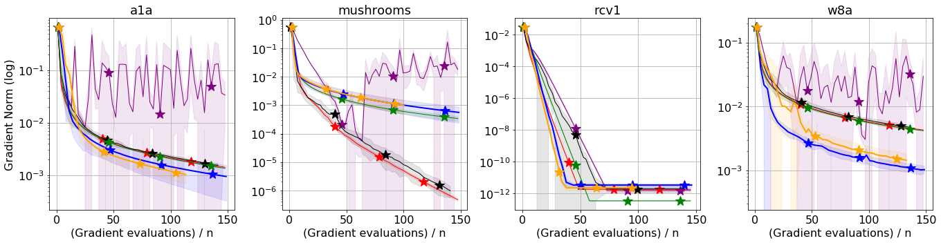
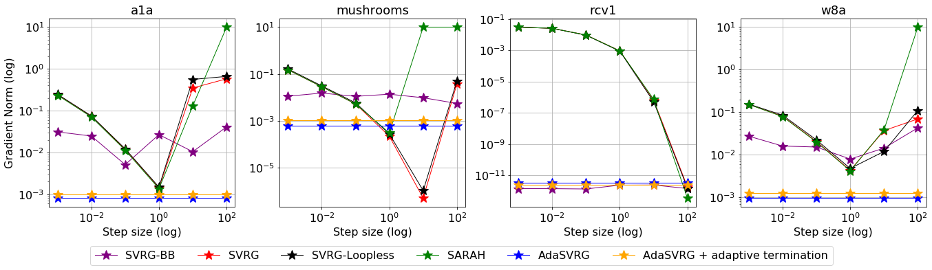
() Logistic loss

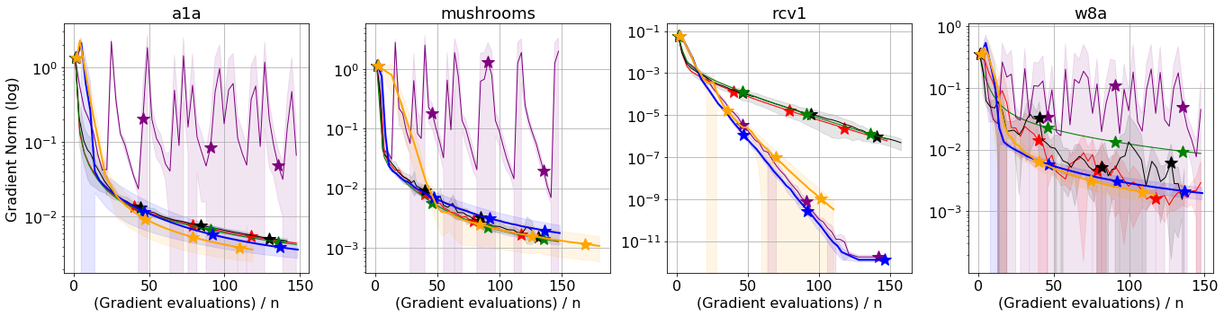
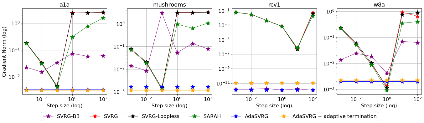
() Huber loss

Figure 1: Comparison of AdaSVRG against SVRG variants, SVRG-BB and SARAH with batch-size = $64$ for logistic loss (top 2 rows) and Huber loss (bottom 2 rows). For both losses, we compare AdaSVRG against the best-tuned variants, and show the sensitivity to step-size (we limit the gradient norm to a maximum value of 10).

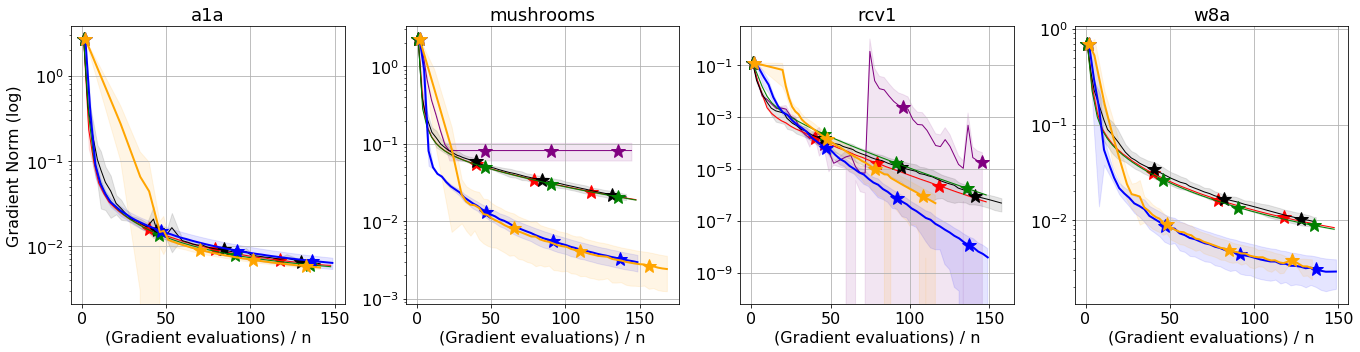
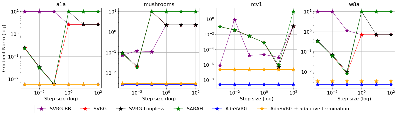
() Squared loss

Figure 2: Comparison of AdaSVRG against SVRG variants, SVRG-BB and SARAH with batch-size = $64$ for squared loss We compare AdaSVRG against the best-tuned variants, and show the sensitivity to step-size (we limit the gradient norm to a maximum value of 10). In cases where SVRG-BB diverged, we remove these curves.

We first describe the practical considerations for implementing AdaSVRG and then evaluate its performance on real and synthetic datasets. We do not use projections in our experiments as these problems have an unconstrained $w^{*}$ with finite norm (we thus assume $D$ is big enough to include it), and that we empirically observed that our iterates always stayed bounded, thus not requiring any projection.

Implementing AdaSVRG: Though our theoretical results hold for any bounded sequence of step-sizes, its choice affects the practical performance of AdaGrad (Vaswani et al.,, 2020) (and hence AdaSVRG). Theoretically, the optimal step-size minimizing the bound in Lemma 1 is given by $\eta^{*}=\frac{D}{\sqrt{2}}$. Since we do not have access to $D$, we use the following heuristic to set the step-size for each outer-loop of AdaSVRG. In outer-loop $k$, we approximate $D$ by $\|w_{k}-w^{*}\|$, that can be bounded using the co-coercivity of smooth convex functions as $\|w_{k}-w^{*}\|\geq\nicefrac{{1}}{{L_{\text{max}}}}\|\nabla f(w_{k})\|$ (Nesterov,, 2004, Thm. 2.1.5 (2.1.8)). We have access to $\nabla f(w_{k})$ for the current outer-loop, and store the value of $\nabla f(w_{k-1})$ in order to approximate the smoothness constant. Specifically, by co-coercivity, $L_{\text{max}}\geq L_{k}\coloneqq\frac{\|\nabla f(w_{k})-\nabla f(w_{k-1})\|}{\|w_{k}-w_{k-1}\|}$. Putting these together, $\eta_{k}=\frac{\|\nabla f(w_{k})\|}{\sqrt{2}\,\max_{i=0,\dots,k}L_{i}}$. Although a similar heuristic could be used to estimate $L_{\text{max}}$ for SVRG or SARAH, the resulting step-size is larger than $1/L_{\text{max}}$ implying that it would not have any theoretical guarantee, while our results hold for any bounded sequence of step-sizes. Although Algorithm 1 requires setting $w_{k+1}$ to be the average of the inner-loop iterates, we use the last-iterate and set $w_{k}=x_{m_{k}}$, as this is a more common choice (Johnson and Zhang,, 2013; Tan et al.,, 2016) and results in better empirical performance. We compare two variants of AdaSVRG, with (i) fixed-size inner-loop Algorithm 1 and (ii) adaptive termination Algorithm 3. We handle a general batch-size $b$, and set $m=\nicefrac{{n}}{{b}}$ for Algorithm 1. This is a common practical choice (Babanezhad Harikandeh et al.,, 2015; Gower et al.,, 2020; Kovalev et al.,, 2020). For Algorithm 3, the burn-in phase consists of $\nicefrac{{n}}{{2b}}$ iterations and $M=\nicefrac{{10n}}{{b}}$.

Evaluating AdaSVRG: In order to assess the effectiveness of AdaSVRG, we experiment with binary classification on standard LIBSVM datasets (Chang and Lin,, 2011). In particular, we consider $\ell_{2}$-regularized problems (with regularization set to $\nicefrac{{1}}{{n}}$) with three losses - logistic loss, the squared loss or the Huber loss. For each experiment we plot the median and standard deviation across 5 independent runs. In the main paper, we show the results for four of the datasets and relegate the results for the three others to Appendix L. Similarly, we consider batch-sizes in the range $[1,8,64,128]$, but only show the results for $b=64$ in the main paper.

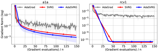
Figure 4: Poor performance of best-tuned step-size (after grid-search) AdaGrad compared to SVRG and AdaSVRG on logistic regression problems with batch size 64 on two example datasets

We compare the AdaSVRG variants against SVRG (Johnson and Zhang,, 2013), loopless-SVRG (Kovalev et al.,, 2020), SARAH (Nguyen et al.,, 2017), and SVRG-BB (Tan et al.,, 2016), the only other tune-free VR method. Since each of these methods requires a step-size, we search over the grid $[10^{-3},10^{-2},10^{-1},1,10,100]$, and select the best step-size for each algorithm and each experiment. As is common, we set $m=\nicefrac{{n}}{{b}}$ for each of these methods. We note that though the theoretical results of SVRG-BB require a small $O(1/\kappa^{2})$ step-size and $O(\kappa^{2})$ inner-loops, Tan et al., (2016) recommends setting $m=O(n)$ in practice. Since AdaGrad results in the slower $O(1/\epsilon^{2})$ rate (Levy et al.,, 2018; Vaswani et al.,, 2020) compared to the $O(n+\frac{1}{\epsilon})$ rate of VR methods, we do not include it in the main paper. We demonstrate the poor performance of AdaGrad on two example datasets in Fig. 4 in Appendix L.

We plot the gradient norm of the training objective (for the best step-size) against the number of gradient evaluations normalized by the number of examples. We show the results for the logistic loss (Fig. 1), Huber loss (Fig. 1), and squared loss (Fig. 2). Our results show that (i) both variants of AdaSVRG (without any step-size tuning) are competitive with the other best-tuned VR methods, often out-performing them or matching their performance; (ii) SVRG-BB often has an oscillatory behavior, even for the best step-size; and (iii) the performance of AdaSVRG with adaptive termination (that has superior theoretical complexity) is competitive with that of the practically useful $O(n)$ fixed inner-loop setting.

In order to evaluate the effect of the step-size on a method’s performance, we plot the gradient norm after $50$ outer-loops vs step-size for each of the competing methods. For the AdaSVRG variants, we set the step-size according to the heuristic described earlier. For the logistic loss (Fig. 1()), Huber loss (Fig. 1()) and squared loss (Fig. 2()), we observe that (i) the performance of typical VR methods heavily depends on the choice of the step-size; (ii) the step-size corresponding to the minimum loss is different for each method, loss and dataset; and (iii) AdaSVRG with the step-size heuristic results in competitive performance. Additional experiments in Appendix L confirm that the good performance of AdaSVRG is consistent across losses, batch-sizes and datasets.

6 Discussion

Although there have been numerous papers on VR methods in the past ten years, all of the provably convergent methods require knowledge of problem-dependent constants such as $L$. On the other hand, there has been substantial progress in designing adaptive gradient methods that have effectively replaced SGD for training ML models. Unfortunately, this progress has not been leveraged for developing better VR methods. Our work is the first to marry these lines of literature by designing AdaSVRG, that achieves a gradient complexity comparable to typical VR methods, but without needing to know the objective’s smoothness constant. Our results illustrate that it is possible to design principled techniques that can “painlessly” reduce the variance, achieving good theoretical and practical performance. We believe that our paper will help open up an exciting research direction. In the future, we aim to extend our theory to the strongly-convex setting.

7 Acknowledgments

We would like to thank Raghu Bollapragada for helpful discussions. This research was partially supported by the Canada CIFAR AI Chair Program, a Google Focused Research award and an IVADO postdoctoral scholarship. Simon Lacoste-Julien is a CIFAR Associate Fellow in the Learning in Machines & Brains program.

 
Supplementary material
 

Organization of the Appendix

• Definitions

• Heuristic for adaptivity to over-parameterization

• Proof of Lemma

• Main Proposition

• Proof of Theorem 1

• Proof of Theorem 2

• Proof of Theorem

• Proof of Theorem 4

• Helper Lemmas

• Counter-example for line-search for SVRG

• Additional Experiments

Appendix A Definitions

Our main assumptions are that each individual function $f_{i}$ is differentiable and $L_{i}$-smooth, meaning that for all $v$ and $w$,

$$f_{i}(v) \leq f_{i}(w)+\langle\nabla f_{i}(w),\,v-w\rangle+\frac{L_{i}}{2}\left\|v-w\right\|^{2},$$ (Individual Smoothness)

which also implies that $f$ $L_{\max}$-smooth, where $L_{\max}$ is the maximum smoothness constant of the individual functions. We also assume that $f$ is convex, meaning that for all $v$ and $w$,

$$f(v) \geq f(w)-\langle\nabla f(w),w-v\rangle.$$ (Convexity)

Appendix B Heuristic for adaptivity to over-parameterization

Input: $x_{1}$ (initial point), $T$ (iteration budget), $M$ (maximum inner loops), $\theta$ (adaptive termination parameter)

Phase 1: AdaGrad

$G_{0}\leftarrow\mathbf{0}$

for $t\leftarrow 1$ to $T$ do

       Sample $i_{t}\sim\text{Uniform}\{1,2,\ldots n\}$

       $\eta_{t}\leftarrow$ Compute step-size

       $G_{t}=G_{t-1}+\left\|g_{t}\right\|^{2}$

       $A_{t}=G_{t}^{1/2}$

       if $t$ mod $2$ $==0$ and $t\geq 2n$ then

             $R=\frac{\|G_{t}\|^{2}_{*}-\|G_{t/2}\|^{2}_{*}}{\|G_{t/2}\|^{2}_{*}}$

             if $R\geq\theta$ then

                   Terminate and switch to AdaSVRG

             end if

            

       end if

      $x_{t+1}=\Pi_{X,A_{t}}\left(x_{t}-\eta_{k}A_{t}^{-1}g_{t}\right)$

end for

Phase 2: AdaSVRG

$w_{K}$ = Algorithm 3($x_{t}$, $\lfloor\frac{T-t}{n}\rfloor$, $\theta$, $M$)

Return $w_{K}$

Algorithm 4 Hybrid AdaGrad-AdaSVRG

In this section, we reason that the poor empirical performance of SVRG when training over-parameterized models (Defazio and Bottou,, 2019) can be partially explained by the interpolation property (Schmidt and Le Roux,, 2013; Ma et al.,, 2018; Vaswani et al., 2019a, ) satisfied by these models (Zhang et al.,, 2017). In particular, we focus on smooth convex losses, but assume that the model is capable of completely fitting the training data, and that $w^{*}$ lies in the interior of $X$. For example, these properties are simultaneously satisfied when minimizing the squared hinge-loss for linear classification on separable data or unregularized kernel regression (Belkin et al.,, 2019; Liang et al.,, 2020) with $\|w^{*}\|\leq 1$.

Formally, the interpolation condition means that the gradient of each $f_{i}$ in the finite-sum converges to zero at an optimum. Additionally, we assume that each function $f_{i}$ has finite minimum $f_{i}^{*}$. If the overall objective $f$ is minimized at $w^{*}$, $\nabla f(w^{*})=0$, then for all $f_{i}$ we have $\nabla f_{i}(w^{*})=0$. Since the interpolation property is rarely exactly satisfied in practice, we allow for a weaker version that uses $\zeta^{2}\coloneqq\mathbb{E}_{i}[f^{*}-f_{i}^{*}]\in[0,\infty)$ (Loizou et al.,, 2020; Vaswani et al.,, 2020) to measure the extent of the violation of interpolation. If $\zeta^{2}=0$, interpolation is exactly satisfied.

When $\zeta^{2}=0$, both constant step-size SGD and AdaGrad have a gradient complexity of $O(1/\epsilon)$ in the smooth convex setting (Schmidt and Le Roux,, 2013; Vaswani et al., 2019a, ; Vaswani et al.,, 2020). In contrast, typical VR methods have an $\tilde{O}(n+\frac{1}{\epsilon})$ complexity. For example, both SVRG and AdaSVRG require computing the full gradient in every outer-loop, and will thus unavoidably suffer an $\Omega(n)$ cost. For large $n$, typical VR methods will thus be necessarily slower than SGD when training models that can exactly interpolate the data. This provides a partial explanation for the ineffectiveness of VR methods when training over-parameterized models. When $\zeta^{2}>0$, AdaGrad has an $O(1/\epsilon+\zeta/\epsilon^{2})$ rate (Vaswani et al.,, 2020). Here $\zeta$, the violation of interpolation plays the role of noise and slows down the convergence to an $O(1/\epsilon^{2})$ rate. On the other hand, AdaSVRG results in an $\tilde{O}(n+1/\epsilon)$ rate, regardless of $\zeta$.

Following the reasoning in Section 4, if an algorithm can detect the slower convergence of AdaGrad and switch from AdaGrad to AdaSVRG, it can attain a faster convergence rate. It is straightforward to show that AdaGrad has a a similar phase transition as Theorem 4 when interpolation is only approximately satisfied. This enables the use of the test in Section 4 to terminate AdaGrad and switch to AdaSVRG, resulting in the hybrid algorithm described in Algorithm 4. If the diagnostic test can detect the phase transition accurately, Algorithm 4 will attain an $O(1/\epsilon)$ convergence when interpolation is exactly satisfied (no switching in this case). When interpolation is only approximately satisfied, it will result in an $O(1/\epsilon)$ convergence for $\epsilon\geq\zeta$ (corresponding to the AdaGrad rate in the deterministic phase) and will attain an $O(1/\zeta^{2}+((n+1/\epsilon)\log(\zeta/\epsilon))$ convergence thereafter (corresponding to the AdaSVRG rate). This implies that Algorithm 4 can indeed obtain the best of both worlds between AdaGrad and AdaSVRG.

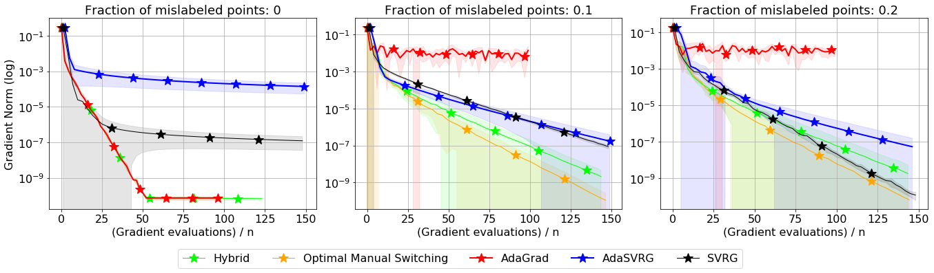
Figure 3: Comparison of AdaGrad, AdaSVRG and Algorithm 4 (denoted "Hybrid" in the plots) with logistic loss and batch-size $64$ on datasets with different fraction of mislabeled data-points. Interpolation is exactly satisfied for the left-most plot.

Evaluating Algorithm 4: We use synthetic experiments to demonstrate the effect of interpolation on the convergence of stochastic and VR methods. Following the protocol in (Meng et al.,, 2020), we generate a linearly separable dataset with $n=10^{4}$ data points of dimension $d=200$ and train a linear model with a convex loss. This setup ensures that interpolation is satisfied, but allows to eliminate other confounding factors such as non-convexity and other implementation details. In order to smoothly violate interpolation, we show results with a mislabel fraction of points in the grid $[0,0.1,0.2]$.

We use AdaGrad as a representative (fully) stochastic method, and to eliminate possible confounding because of its step-size, we set it using the stochastic line-search procedure (Vaswani et al.,, 2020). We compare the performance of AdaGrad, SVRG, AdaSVRG and the hybrid AdaGrad-AdaSVRG (Algorithm 4) each with a budget of $50$ epochs (passes over the data). For SVRG, as before, we choose the best step-size via a grid-search. For AdaSVRG, we use the fixed-size inner-loop variant and the step-size heuristic described earlier. In order to evaluate the quality of the “switching” metric in Algorithm 4, we compare against a hybrid method referred to as “Optimal Manual Switching” in the plots. This method runs a grid-search over switching points - after epoch $\{1,2,\ldots,50\}$ and chooses the point that results in the minimum loss after $50$ epochs.

In Fig. 3, we plot the results for the logistic loss using a batch-size of $64$ (refer to Appendix L for other losses and batch-sizes). We observe that (i) when interpolation is exactly satisfied (no mislabeling), AdaGrad results in superior performance over SVRG and AdaSVRG, confirming the theory in Appendix B. In this case, both the optimal manual switching and Algorithm 4 do not switch; (ii) when interpolation is not exactly satisfied (with $10\%,20\%$ mislabeling), the AdaGrad progress slows down to a stall in a neighbourhood of the solution, whereas both SVRG and AdaSVRG converge to the solution; (iii) in both cases, Algorithm 4 detects the slowdown in AdaGrad and switches to AdaSVRG, resulting in competitive performance with the optimal manual switching. For all three datasets, Algorithm 4 matches or out-performs the better of AdaGrad and AdaSVRG, showing that it can achieve the best-of-both-worlds.

In Appendix L, we evaluate the performance of these methods for binary classification with kernel mappings on the mushrooms and ijcnn datasets. This experimental setup can also simultaneously ensure convexity and interpolation (Vaswani et al., 2019b, ), and we observe the same favourable behaviour of the proposed hybrid algorithm.

Appendix C Algorithm in general case

We restate Algorithm 1 to handle the full matrix and diagonal variants. The only difference is in the initialization and update of $G_{t}$.

Input: $w_{0}$ (initial point), $K$ (outer-loops), $m$ (inner-loops)

for $k\leftarrow 0$ to $K-1$ do

       Compute full gradient $\nabla f(w_{k})$

       $\eta_{k}\leftarrow$ Compute step-size

       Initialize: $x_{1}=w_{k}$ and $G_{0}=\begin{cases}0&\text{ (scalar variant)}\\ \delta I&\text{ (full matrix and diagonal variants)}\end{cases}$.

       for $t\leftarrow 1$ to $m$ do

             Sample $i_{t}\sim\text{Uniform}\{1,2,\ldots n\}$

             $g_{t}=\nabla f_{i_{t}}(x_{t})-\nabla f_{i_{t}}(w_{k})+\nabla f(w_{k})$

             $G_{t}=G_{t-1}+\begin{cases}\left\|g_{t}\right\|^{2}&\text{ (scalar variant)}\\ \operatorname{diag}\left(g_{t}g_{t}^{\top}\right)&\text{ (diagonal variant)}\\ g_{t}g_{t}^{\top}&\text{ (full matrix variant)}\end{cases}$

             $A_{t}=G_{t}^{1/2}$

             $x_{t+1}=\Pi_{X,A_{t}}\left(x_{t}-\eta_{k}A_{t}^{-1}g_{t}\right)$

       end for

      $w_{k+1}=\frac{1}{m}\sum_{t=1}^{m}x_{t}$

end for

Return $\bar{w}_{K}=\frac{1}{K}\sum_{k=1}^{K}w_{k}$

Algorithm 5 AdaSVRG with fixed-sized inner-loop

Appendix D Proof of Lemma 1

We restate Lemma 1 to handle the three variants of AdaSVRG.

Lemma 2 (AdaSVRG with single outer-loop).

Assuming (i) convexity of $f$, (ii) $L_{\max}$-smoothness of $f_{i}$ and (iii) bounded feasible set with diameter $D$. For the scalar variant, defining $\rho:=\big{(}\frac{D^{2}}{\eta_{k}}+2\eta_{k}\big{)}\sqrt{L_{\text{max}}}$, for any outer loop $k$ of AdaSVRG, with (a) inner-loop length $m_{k}$ and (b) step-size $\eta_{k}$, $\displaystyle\mathbb{E}[f(w_{k+1})-f^{*}]\leq\frac{\rho^{2}}{m_{k}}+\frac{\rho\sqrt{\mathbb{E}[f(w_{k})-f^{*}]}}{\sqrt{m_{k}}}$ For the full matrix and diagonal variants, setting $\rho^{\prime}:=\left(\frac{D^{2}}{\eta_{k}}+2\eta_{k}\right)\sqrt{dL_{\text{max}}}$, $\displaystyle\mathbb{E}[f(w_{k+1})-f^{*}]\leq\frac{(\rho^{\prime})^{2}+\sqrt{\nicefrac{{d\delta}}{{4L_{\text{max}}}}}}{m_{k}}+\frac{\rho^{\prime}\sqrt{\mathbb{E}[f(w_{k})-f^{*}]}}{\sqrt{m_{k}}}$

Proof.

For any of the three variants, we have, for any outer loop iteration $k$ and any inner loop iteration $t$,

$$\left\|x_{t+1}-w^{*}\right\|^{2}_{A_{t}} =\left\|P_{X,A_{t}}(x_{t}-\eta_{k}A_{t}^{-1}g_{k})-P_{X,A_{t}}(w^{*})\right\|_{A_{t}}^{2}$$ (2)

$$\leq\left\|x_{t}-\eta_{k}A^{-1}_{t}g_{k}-w^{*}\right\|^{2}_{A_{t}}$$ (3)

$$=\left\|x_{t}-w^{*}\right\|^{2}_{A_{t}}-2\eta_{k}\langle g_{t},\,x_{t}-w^{*}\rangle+\eta_{k}^{2}\left\|g_{t}\right\|^{2}_{A_{t}^{-1}}$$ (4)

where the inequality follows from Reddi et al., (2018, Lemma 4) Dividing by $\eta_{k}$, rearranging and summing over all inner loop iterations at stage $k$ gives

$$2\sum_{t=1}^{m_{k}}\langle g_{t},\,x_{t}-w^{*}\rangle \leq\sum_{t=1}^{m_{k}}\left\|x_{t}-w^{*}\right\|^{2}_{\frac{A_{t}}{\eta_{k}}-\frac{A_{t-1}}{\eta_{k}}}+\sum_{t=1}^{m_{k}}\eta_{k}\left\|g_{t}\right\|^{2}_{A_{t}^{-1}}$$ (5)

$$\leq\frac{D^{2}}{\eta_{k}}\mathrm{Tr}(A_{m_{k}})+2\eta_{k}\mathrm{Tr}(A_{m_{k}})$$ (Lemma 3 and Lemma 4 )

$$=\left(\frac{D^{2}}{\eta_{k}}+2\eta_{k}\right)\mathrm{Tr}(A_{m_{k}})$$ (6)

By Lemma 4, we have that $\mathsf{Tr}\mathclose{{}\left(A_{m_{k}}}\right)\leq\sqrt{\sum_{t=1}^{m_{k}}\left\|g_{t}\right\|^{2}}$ in the scalar case, and $\mathsf{Tr}\mathclose{{}\left(A_{m_{k}}}\right)\leq\sqrt{d}\sqrt{\sum_{t=1}^{m_{k}}\left\|g_{t}\right\|^{2}+d\delta}$ in the full matrix and diagonal variants. Therefore we set

$$a^{\prime}=\begin{cases}\frac{1}{2}\big{(}\frac{D^{2}}{\eta_{k}}+2\eta_{k}\big{)}&\text{(scalar variant)}\\ \frac{1}{2}\big{(}\frac{D^{2}}{\eta_{k}}+2\eta_{k}\big{)}\sqrt{d}&\text{(full matrix and diagonal variants)}\end{cases}$$

and

$$b=\begin{cases}0&\text{(scalar variant)}\\ d\delta&\text{(full matrix and diagonal variants)}\end{cases}$$

Going back to the above inequality and taking expectation we get

$$\sum_{t=1}^{m_{k}}\langle\nabla f(x_{t}),\,x_{t}-w^{*}\rangle \leq a^{\prime}\,\mathbb{E}\left[\sqrt{\sum_{t=1}^{m_{k}}\left\|g_{t}\right\|^{2}+b}\right]$$ (7)

Using convexity of $f$ yields

$$\sum_{t=1}^{m_{k}}\mathbb{E}[f(x_{t})-f^{*}] \leq a^{\prime}\mathbb{E}\bigg{[}\sqrt{\sum_{t=1}^{m_{k}}\left\|g_{t}\right\|^{2}+b}\bigg{]}$$ (8)

$$\leq a^{\prime}\sqrt{\mathbb{E}\big{[}\sum_{t=1}^{m_{k}}\left\|g_{t}\right\|^{2}+b\big{]}}$$ (9)

$$=a^{\prime}\sqrt{\sum_{t=1}^{m_{k}}\mathbb{E}[\left\|g_{t}\right\|^{2}]+b}$$ (10)

where the second inequality comes from Jensen’s inequality applied to the (concave) square root function. Now, from Kovalev et al., (2020),

$$\mathbb{E}[\left\|g_{t}\right\|^{2}]\leq 4L_{\text{max}}\mathbb{E}[f(w_{k})-f^{*}]+4L_{\text{max}}\mathbb{E}[f(x_{t})-f^{*}]$$ (11)

Going back to the previous equation, squaring and setting $\tau=a^{\prime}\sqrt{4L_{\text{max}}}$ we get

$$\left(\sum_{t=1}^{m_{k}}\mathbb{E}[f(x_{t})-f^{*}]\right)^{2}\leq\tau^{2}\left(\sum_{t=1}^{m_{k}}\mathbb{E}[f(x_{t})-f^{*}]+m_{k}\mathbb{E}[f(w_{k})-f^{*}]+\frac{b}{4L_{\text{max}}}\right)$$ (12)

Using Lemma 5,

$$\sum_{t=1}^{m_{k}}\mathbb{E}[f(x_{t})-f^{*}]\leq\tau^{2}+\tau\sqrt{m_{k}\mathbb{E}[f(w_{k})-f^{*}]+\frac{b}{4L_{\text{max}}}}\leq\tau^{2}+\tau\sqrt{\frac{b}{4L_{\text{max}}}}+\tau\sqrt{m_{k}\mathbb{E}[f(w_{k})-f^{*}]}$$ (13)

Finally, using Jensen’s inequality we get

$$\mathbb{E}\left[f(w_{k+1})-f^{*}\right] =\mathbb{E}\left[f\left(\frac{1}{m_{k}}\sum_{t=1}^{m_{k}}x_{t}\right)-f^{*}\right]$$ (14)

$$\leq\frac{\tau^{2}+\tau\sqrt{\frac{b}{4L_{\text{max}}}}}{m_{k}}+\frac{\tau\sqrt{\mathbb{E}[f(w_{k})-f^{*}]}}{\sqrt{m_{k}}}$$ (15)

which concludes the proof by noticing that by definition $\tau=\rho$ in the scalar case and $\tau=\rho^{\prime}$ in the full matrix and diagonal cases.

∎

Appendix E Main Proposition

We first state the main proposition for the three variants of AdaSVRG, which we later use for proving theorems.

Proposition 2.

Assuming (i) convexity of $f$ (ii) $L_{\text{max}}$-smoothness of $f$ (iii) bounded feasible set (iv) $\eta_{k}\in[\eta_{\text{min}},\eta_{\text{max}}]$ (v) $m_{k}=m$ for all $k$, then for the scalar variant,

$$\mathbb{E}[f(\bar{w}_{K})-f^{*}]\leq\frac{\rho^{2}(1+\sqrt{5})}{m}+\frac{\rho\sqrt{2\left(f(w_{0})-f^{*}\right)}}{\sqrt{mK}}$$

and for the full matrix and diagonal variants,

$$\mathbb{E}[f(\bar{w}_{K})-f^{*}]\leq\frac{(\rho^{\prime})^{2}(1+\sqrt{5})+2\rho^{\prime}\sqrt{\nicefrac{{d\delta}}{{L_{\text{max}}}}}}{m}+\frac{\rho^{\prime}\sqrt{2\left(f(w_{0})-f^{*}\right)}}{\sqrt{mK}}$$

where $\bar{w}_{K}=\frac{1}{K}\sum_{k=1}^{K}w_{k}$, $\rho=\left(\frac{D^{2}}{\eta_{\text{min}}}+2\eta_{\text{max}}\right)\sqrt{L_{\text{max}}}$ and $\rho^{\prime}=\left(\frac{D^{2}}{\eta_{\text{min}}}+2\eta_{\text{max}}\right)\sqrt{dL_{\text{max}}}$.

Proof.

As in the previous proof we define

$$b=\begin{cases}0&\text{(scalar variant)}\\ d\delta&\text{(full matrix and diagonal variants)}\end{cases}$$

and

$$\tau=\begin{cases}\rho&\text{(scalar variant)}\\ \rho^{\prime}&\text{(full matrix and diagonal variants)}\end{cases}$$

Using the result from Lemma 1 and letting $\Delta_{k}\coloneqq\mathbb{E}[f(w_{k})-f^{*}]$, we have,

$$\Delta_{k+1}\leq\frac{\tau^{2}+\tau\sqrt{\frac{b}{4L_{\text{max}}}}}{m}+\tau\frac{\sqrt{\Delta_{k}}}{\sqrt{m}}$$ (16)

Squaring gives

$$\Delta_{k+1}^{2} \leq\left(\frac{\tau^{2}+\tau\sqrt{\frac{b}{4L_{\text{max}}}}}{m}+\frac{\tau\sqrt{\Delta_{k}}}{\sqrt{m}}\right)^{2}\leq 2\frac{\left(\tau^{2}+\tau\sqrt{\frac{b}{4L_{\text{max}}}}\right)^{2}}{m^{2}}+2\frac{\tau^{2}}{m}\Delta_{k}\leq 4\frac{\tau^{2}}{m^{2}}+4\frac{\tau^{2}\frac{b}{4L_{\text{max}}}}{m^{2}}+2\frac{\tau^{2}}{m}\Delta_{k}$$ (17)

which we can rewrite as

$$\Delta_{k+1}^{2}-2\frac{\tau^{2}}{m}\Delta_{k+1}\leq 4\frac{\tau^{4}}{m^{2}}+2\frac{\tau^{2}}{m}(\Delta_{k}-\Delta_{k+1})+4\frac{\tau^{2}b}{L_{\text{max}}m^{2}}$$ (18)

Since $\Delta_{k+1}^{2}-2\frac{\tau^{2}}{m}\Delta_{k+1}=(\Delta_{k+1}-\frac{\tau^{2}}{m})^{2}-\frac{\tau^{4}}{m^{2}}$, we get

$$(\Delta_{k+1}-\frac{\tau^{2}}{m})^{2}\leq 5\frac{\tau^{4}}{m^{2}}+2\frac{\tau^{2}}{m}(\Delta_{k}-\Delta_{k+1})+4\frac{\tau^{2}b}{L_{\text{max}}m^{2}}$$ (19)

Summing this gives

$$\sum_{k=0}^{K-1}\left(\Delta_{k+1}-\frac{\tau^{2}}{m}\right)^{2} \leq\left(5\tau^{4}+4\frac{\tau^{2}b}{L_{\text{max}}}\right)\frac{K}{m^{2}}+2\frac{\tau^{2}}{m}\sum_{k=0}^{K-1}(\Delta_{k}-\Delta_{k+1})$$ (20)

$$\leq\left(5\tau^{4}+4\frac{\tau^{2}b}{L_{\text{max}}}\right)\frac{K}{m^{2}}+2\frac{\tau^{2}}{m}\Delta_{0}$$ (21)

Using Jensen’s inequality on the (concave) square root function gives

$$\frac{1}{K}\sum_{k=0}^{K-1}(\Delta_{k+1}-\frac{\tau^{2}}{m})\leq\frac{1}{K}\sum_{k=0}^{K-1}\sqrt{\left(\Delta_{k+1}-\frac{\tau^{2}}{m}\right)^{2}}\leq\sqrt{\frac{1}{K}\sum_{k=0}^{K-1}\left(\Delta_{k+1}-\frac{\tau^{2}}{m}\right)^{2}}$$ (22)

going back to the previous inequality this gives

$$\frac{1}{K}\sum_{k=0}^{K-1}(\Delta_{k+1}-\frac{\tau^{2}}{m}) \leq\sqrt{\left(5\tau^{4}+4\frac{\tau^{2}b}{L_{\text{max}}}\right)\frac{1}{m^{2}}+2\tau^{2}\frac{\Delta_{0}}{mK}}$$ (23)

$$\leq\frac{\tau^{2}\sqrt{5}+2\tau\sqrt{\nicefrac{{b}}{{L_{\text{max}}}}}}{m}+\frac{\tau\sqrt{2\Delta_{0}}}{\sqrt{mK}}$$ (24)

which we can rewrite

$$\frac{1}{K}\sum_{k=0}^{K-1}\Delta_{k+1}\leq\frac{\tau^{2}(1+\sqrt{5})+2\tau\sqrt{\nicefrac{{b}}{{L_{\text{max}}}}}}{m}+\frac{\tau\sqrt{2\Delta_{0}}}{\sqrt{mK}}$$ (25)

Setting $\bar{w}_{K}=\frac{1}{K}\sum_{k=0}^{K-1}w_{k}$ and using Jensen’s inequality on the convex function $f$, we get

$$\mathbb{E}[f(\bar{w}_{K})-f^{*}]\leq\frac{\tau^{2}(1+\sqrt{5})+2\tau\sqrt{\nicefrac{{b}}{{L_{\text{max}}}}}}{m}+\frac{\tau\sqrt{2\Delta_{0}}}{\sqrt{mK}}$$ (26)

which concludes the proof. ∎

Appendix F Proof of Theorem 1

For the remainder of the appendix we define $\rho^{\prime}\coloneqq\big{(}\frac{D^{2}}{\eta_{\text{min}}}+2\eta_{\text{max}}\big{)}\sqrt{dL_{\text{max}}}$. We restate and prove Theorem 1 for all three variants of AdaSVRG.

Theorem 5 (AdaSVRG with fixed-size inner-loop).

Under the same assumptions as Lemma 1, AdaSVRG with (a) step-sizes $\eta_{k}\in[\eta_{\text{min}},\eta_{\text{max}}]$, (b) inner-loop size $m_{k}=n$ for all $k$, results in the following convergence rate after $K\leq n$ iterations. For the scalar variant, $\displaystyle\mathbb{E}[f(\bar{w}_{K})-f^{*}]\leq\frac{\rho^{2}(1+\sqrt{5})+\rho\sqrt{2\left(f(w_{0})-f^{*}\right)}}{K}$ and for the full matrix and diagonal variants, $\displaystyle\mathbb{E}[f(\bar{w}_{K})-f^{*}]\leq\frac{(\rho^{\prime})^{2}(1+\sqrt{5})+2\rho^{\prime}\sqrt{\nicefrac{{d\delta}}{{L_{\text{max}}}}}+\rho^{\prime}\sqrt{2\left(f(w_{0})-f^{*}\right)}}{K},$ where $\bar{w}_{K}=\frac{1}{K}\sum_{k=1}^{K}w_{k}$.

Proof.

We have $\frac{1}{m}=\frac{1}{n}\leq\frac{1}{K}$ by the assumption. Using the result of Proposition 2 for the scalar variant we have

$$\mathbb{E}[f(\bar{w}_{K})-f^{*}] \leq\frac{\rho^{2}(1+\sqrt{5})}{m}+\frac{\rho\sqrt{2\Delta_{0}}}{\sqrt{mK}}$$ (27)

$$\leq\frac{\rho^{2}(1+\sqrt{5})}{K}+\frac{\rho\sqrt{2\Delta_{0}}}{K}$$ (28)

Using the result of Proposition 2 for the full matrix and diagonal variants we have

$$\mathbb{E}[f(\bar{w}_{K})-f^{*}] \leq\frac{(\rho^{\prime})^{2}(1+\sqrt{5})+2\rho^{\prime}\sqrt{\nicefrac{{d\delta}}{{L_{\text{max}}}}}}{m}+\frac{\rho^{\prime}\sqrt{2\Delta_{0}}}{\sqrt{mK}}$$ (29)

$$\leq\frac{(\rho^{\prime})^{2}(1+\sqrt{5})+2\rho^{\prime}\sqrt{\nicefrac{{d\delta}}{{L_{\text{max}}}}}}{K}+\frac{\rho^{\prime}\sqrt{2\Delta_{0}}}{K}$$ (30)

∎

Corollary 1.

Under the assumptions of Theorem 1, the computational complexity of AdaSVRG to reach $\epsilon$-accuracy is $O\left(\frac{n}{\epsilon}\right)$ when $\epsilon\geq\frac{\rho^{2}(1+\sqrt{5})+\rho\sqrt{2\left(f(w_{0})-f^{*}\right)}}{n}$ for the scalar variant and when $\epsilon\geq\frac{(\rho^{\prime})^{2}(1+\sqrt{5})+2\rho^{\prime}\sqrt{\nicefrac{{d\delta}}{{L_{\text{max}}}}}+\rho^{\prime}\sqrt{2\left(f(w_{0})-f^{*}\right)}}{n}$ for the full matrix and diagonal variants.

Proof.

We deal with the scalar variant first. Let $c=\rho^{2}(1+\sqrt{5})+\rho\sqrt{2\left(f(w_{0})-f^{*}\right)}$. By the previous theorem, to reach $\epsilon$-accuracy we require

$$\frac{c}{K}\leq\epsilon$$ (31)

We thus require $O\left(\frac{1}{\epsilon}\right)$ outer loops to reach $\epsilon$-accuracy. For $m_{k}=n$, $3n$ gradients are computed in each outer loop, thus the computational complexity is indeed $O\left(\frac{n}{\epsilon}\right)$.

The condition $\epsilon\geq\frac{c}{n}$ follows from the assumption that $K\leq n$.

The proof for the full matrix and diagonal variants is similar by taking $c=(\rho^{\prime})^{2}(1+\sqrt{5})+2\rho^{\prime}\sqrt{\nicefrac{{d\delta}}{{L_{\text{max}}}}}+\rho^{\prime}\sqrt{2\left(f(w_{0})-f^{*}\right)}$. ∎

Appendix G Proof of Theorem 2

 
         See 2 With the same assumptions as above, the full matrix and diagonal variants of multi-stage AdaSVRG require $O(n\log\frac{1}{\epsilon}+\frac{1}{\epsilon})$ gradient evaluations to reach a $\left((\rho^{\prime})^{2}(1+\sqrt{5})+\rho^{\prime}\sqrt{\nicefrac{{d\delta}}{{L_{\text{max}}}}}\right)\epsilon$-sub-optimality

Proof.

We deal with the scalar variant first. Let $\Delta_{i}:=\mathbb{E}[f(\bar{w}^{i})-f^{*}]$ and $c:=\rho^{2}(1+\sqrt{5})$. Suppose that $K\geq 3$ and $m_{i}=2^{i+1}$, as in the theorem statement. We claim that for all $i$, we have $\Delta_{i}\leq\frac{c}{2^{i}}$. We prove this by induction. For $i=0$, we have

$$\frac{c}{2^{0}} =c=\rho^{2}(1+\sqrt{5})$$ (32)

$$=L_{\text{max}}(1+\sqrt{5})\left(\frac{D^{2}}{\eta}+2\eta\right)^{2}$$ (33)

The quantity $\frac{D^{2}}{\eta}+2\eta$ reaches a minimum for $\eta^{*}=\frac{D}{\sqrt{2}}$. Therefore we can write

$$\frac{c}{2^{0}} =L_{\text{max}}(1+\sqrt{5})\left(\sqrt{2}D+2\frac{D}{\sqrt{2}}\right)^{2}$$ (34)

$$=L_{\text{max}}(1+\sqrt{5})8D^{2}$$ (35)

$$\geq(1+\sqrt{5})8L_{\text{max}}\left\|\bar{w}_{0}-w^{*}\right\|^{2}$$ (36)

$$\geq(1+\sqrt{5})4\left(f(\bar{w}_{0})-f^{*}\right)$$ (smoothness)

$$=(1+\sqrt{5})4\Delta_{0}$$ (37)

$$\geq\Delta_{0}$$ (38)

Now suppose that $\Delta_{i-1}\leq\frac{c}{2^{i-1}}$ for some $i\geq 1$. Using the upper-bound analysis of AdaSVRG in Proposition 2 we get

$$\Delta_{i} \leq\frac{c}{m^{i}}+\frac{\rho\sqrt{2\Delta_{i-1}}}{\sqrt{m^{i}K}}$$ (39)

$$=\frac{c}{2^{i+1}}+\frac{\rho\sqrt{2\Delta_{i-1}}}{\sqrt{2^{i+1}K}}$$ (40)

$$\leq\frac{c}{2^{i+1}}+\frac{\rho\sqrt{2\frac{c}{2^{i-1}}}}{\sqrt{2^{i+1}K}}$$ (induction hypothesis)

$$=\frac{c}{2^{i+1}}+\frac{c}{2^{i+1}}\left(\frac{\rho}{\sqrt{c}}\sqrt{\frac{2^{i+1}}{2^{i-2}K}}\right)$$ (41)

$$\leq\frac{c}{2^{i+1}}+\frac{c}{2^{i+1}}\frac{\rho}{\sqrt{\rho^{2}(1+\sqrt{5})}}\sqrt{\frac{8}{K}}$$ (42)

$$=\frac{c}{2^{i+1}}+\frac{c}{2^{i+1}}\sqrt{\frac{8}{(1+\sqrt{5})K}}$$ (43)

Since $K\geq 3$, one can check that $\frac{8}{(1+\sqrt{5})K}\leq 1$ and thus

$$\Delta_{i}\leq\frac{c}{2^{i+1}}+\frac{c}{2^{i+1}}=\frac{c}{2^{i}}$$ (44)

which concludes the induction step.
At time step $I=\log\frac{1}{\epsilon}$, we thus have $\Delta_{I}\leq\frac{c}{2^{I}}=c\epsilon$. All that is left is to compute the gradient complexity. If we assume that $K=\gamma$ for some constant $\gamma\geq 3$, the gradient complexity is given by

$$\sum_{i=1}^{I}K(n+m^{i}) =\sum_{i=1}^{I}\gamma(n+2^{i+1})$$

$$=\gamma n\log\left(\frac{1}{\epsilon}\right)+\gamma\sum_{i=1}^{I}2^{i+1}$$

$$\leq\gamma n\log\left(\frac{1}{\epsilon}\right)+4\gamma\frac{1}{\epsilon}$$

$$=O\left((n+\frac{1}{\epsilon})\log\frac{1}{\epsilon}\right)$$

which concludes the proof for the scalar variant.
Now we look at the full matrix and diagonal variants. Let’s take $c=(\rho^{\prime})^{2}(1+\sqrt{5})+2\rho^{\prime}\sqrt{\nicefrac{{d\delta}}{{L_{\text{max}}}}}$. Suppose that $K\geq 3$ and $m_{i}=2^{i+1}$, as in the theorem statement. Again, we claim that for all $i$, we have $\Delta_{i}\leq\frac{c}{2^{i}}$. We prove this by induction. For $i=0$, we have

$$\frac{c}{2^{0}} =c=(\rho^{\prime})^{2}(1+\sqrt{5})+2\rho^{\prime}\sqrt{\nicefrac{{d\delta}}{{L_{\text{max}}}}}$$ (45)

$$\geq dL_{\text{max}}(1+\sqrt{5})\left(\frac{D^{2}}{\eta}+2\eta\right)^{2}$$ (46)

The quantity $\frac{D^{2}}{\eta}+2\eta$ reaches a minimum for $\eta^{*}=\frac{D}{\sqrt{2}}$. Therefore we can write

$$\frac{c}{2^{0}} \geq dL_{\text{max}}(1+\sqrt{5})\left(\sqrt{2}D+2\frac{D}{\sqrt{2}}\right)^{2}$$ (47)

$$=dL_{\text{max}}(1+\sqrt{5})8D^{2}$$ (48)

$$\geq d(1+\sqrt{5})8L_{\text{max}}\left\|\bar{w}_{0}-w^{*}\right\|^{2}$$ (49)

$$\geq d(1+\sqrt{5})4\left(f(\bar{w}_{0})-f^{*}\right)$$ (smoothness)

$$=d(1+\sqrt{5})4\Delta_{0}$$ (50)

$$\geq\Delta_{0}$$ (51)

The induction step is exactly the same as in the scalar case. ∎

Appendix H Proof of Theorem 3

We restate and prove Theorem 3 for the three variants of AdaSVRG.

Theorem 6 (AdaSVRG with adaptive-sized inner-loops).

Under the same assumptions as Lemma 1, AdaSVRG with (a) step-sizes $\eta_{k}\in[\eta_{\text{min}},\eta_{\text{max}}]$, (b1) inner-loop size $m_{k}=\frac{\nu}{\epsilon}$ for all $k$ or (b2) inner-loop size $m_{k}=\frac{\nu}{f(w_{k})-f^{*}}$ for outer-loop $k$, results in the following convergence rate, $\displaystyle\mathbb{E}[f(w_{K})-f^{*}]\leq(3/4)^{K}[f(w_{0})-f^{*}].$ where $\nu=4\rho^{2}$ for the scalar variant and $\nu=\left(\frac{2\rho^{\prime}+\sqrt{16(\rho^{\prime})^{2}+12\rho^{\prime}\sqrt{\nicefrac{{d\delta}}{{4L_{\text{max}}}}}}}{3}\right)^{2}$ for the full matrix and diagonal variants.

Proof.

Let us define

$$\alpha=\begin{cases}\frac{1}{2}\big{(}\frac{D^{2}}{\eta_{\text{min}}}+2\eta_{\text{max}}\big{)}&\text{(scalar variant)}\\ \frac{1}{2}\big{(}\frac{D^{2}}{\eta_{\text{min}}}+2\eta_{\text{max}}\big{)}\sqrt{d}&\text{(full matrix and diagonal variants)}\end{cases}$$

and

$$b=\begin{cases}0&\text{(scalar variant)}\\ d\delta&\text{(full matrix and diagonal variants)}\end{cases}$$

Similar to the proof of Lemma 1, for a inner-loop $k$ with $m_{k}$ iterations and $\alpha:=\frac{1}{2}\big{(}\frac{D^{2}}{\eta_{\text{min}}}+2\eta_{\text{max}}\big{)}$ we can show

$$\mathbb{E}\left[\sum_{t=1}^{m_{k}}f(x_{t})-f^{*}\right] \leq\alpha\sqrt{\sum_{t=1}^{m_{k}}\mathbb{E}\left[\left\|g_{t}\right\|^{2}\right]+b}\leq\alpha\sqrt{4L_{\text{max}}\sum_{t=1}^{m_{k}}\mathbb{E}\left[f(x_{t})-f^{*}\right]+4L_{\text{max}}\sum_{t=1}^{m_{k}}\underbrace{\mathbb{E}\left[f(w_{k})-f^{*}\right]}_{\epsilon_{k}}+b}$$ (52)

$$\leq\alpha\sqrt{4L_{\text{max}}\mathbb{E}\left[\sum_{t=1}^{m_{k}}f(x_{t})-f^{*}\right]+4L_{\text{max}}m_{k}\epsilon_{k}+b}$$ (53)

Using Lemma 5 we get

$$\mathbb{E}\left[\sum_{t=1}^{m_{k}}f(x_{t})-f^{*}\right] \leq 4L_{\text{max}}\alpha^{2}+\sqrt{4L_{\text{max}}\alpha^{2}m_{k}\epsilon_{k}+\alpha^{2}b}$$ (54)

If we set $m_{k}=\frac{C}{\epsilon_{k}}$,

$$\mathbb{E}\left[\sum_{t=1}^{m_{k}}f_{t}(x_{t})-f^{*}\right] \leq 4L_{\text{max}}\alpha^{2}+\sqrt{4L_{\text{max}}\alpha^{2}C+\alpha^{2}b}$$ (55)

$$\leq 4L_{\text{max}}\alpha^{2}+\sqrt{4L_{\text{max}}\alpha^{2}C}+\sqrt{\alpha^{2}b}.$$ (56)

Define $a\coloneqq\sqrt{4L_{\text{max}}\alpha^{2}}$ and $\gamma\coloneqq\sqrt{b/4L_{\text{max}}}$, by dividing both sides of (55) by $m_{k}$ and using the definition of $w_{k+1}$,

$$\mathbb{E}\left[f(w_{k+1})-f^{*}\right]\leq\frac{a^{2}+a(\sqrt{C}+\gamma)}{m_{k}}=\left(\frac{a^{2}+a(\sqrt{C}+\gamma)}{C}\right)\mathbb{E}\left[f(w_{k})-f^{*}\right]$$ (57)

Setting $C=\left(\frac{2a+\sqrt{4a^{2}+12(a^{2}+a\gamma)}}{3}\right)^{2}$, we get $\epsilon_{k+1}\leq 3/4\epsilon_{k}$. However, the above proof requires knowing $\epsilon_{k}$. Instead, let us assume a target error of $\epsilon$, implying that we want to have $\mathbb{E}[f(w_{K})-f^{*}]\leq\epsilon$. Going back to (54) and setting $m_{k}=C/\epsilon$, we obtain,

$$\mathbb{E}\left[f(w_{k+1})-f^{*}\right] \leq\frac{a^{2}+a(\sqrt{C\epsilon_{k}/\epsilon}+\gamma)}{m_{k}}=\left(\frac{a^{2}+a(\sqrt{C\epsilon_{k}/\epsilon}+\gamma)}{C}\right)\epsilon$$ (58)

$$\leq\frac{a^{2}\epsilon_{k}+a\sqrt{C\epsilon_{k}/\epsilon}\sqrt{\epsilon_{k}\epsilon}+a\gamma\epsilon_{k}}{C} \epsilon\leq\epsilon_{k} k\leq K$$ (Assuming that for all .)

$$=\left(\frac{a^{2}+a\sqrt{C}+a\gamma}{C}\right)\epsilon_{k}=\left(\frac{a^{2}+a\sqrt{C}+a\gamma}{C}\right)\mathbb{E}\left[f(w_{k})-f^{*}\right]$$ (59)

With $C=\left(\frac{2a+\sqrt{4a^{2}+12(a^{2}+a\gamma)}}{3}\right)^{2}$, we get linear convergence to $\epsilon$-suboptimality. Based on the above we require $K=\mathcal{O}(\log(1/\epsilon))$ outer-loops. However in each outer-loop we need $\mathcal{O}(n+\frac{1}{\epsilon})$ gradient evaluations. All in all, our total computation complexity is of $\mathcal{O}((n+\frac{1}{\epsilon})\log(\frac{1}{\epsilon}))$.
The proof is done by noticing that in the scalar variant, $\gamma=0$ and $a=\rho$ so that

$$C=\left(\frac{2\rho+\sqrt{4\rho^{2}+12\rho^{2}}}{3}\right)^{2}=4\rho^{2}$$

and in the full matrix and diagonal variants, $a=\rho^{\prime}$ and $\gamma=\sqrt{\nicefrac{{d\delta}}{{4L_{\text{max}}}}}$ so that

$$C=\left(\frac{2\rho^{\prime}+\sqrt{16(\rho^{\prime})^{2}+12\rho^{\prime}\sqrt{\nicefrac{{d\delta}}{{4L_{\text{max}}}}}}}{3}\right)^{2}$$

∎

Appendix I Proof of Theorem 4

We restate and prove Theorem 4 for the three variants of AdaGrad.

Theorem 7 (Phase Transition in AdaGrad Dynamics).

Under the same assumptions as Lemma 1 and (iv) $\sigma^{2}$-bounded stochastic gradient variance and defining $T_{0}=\frac{\rho^{2}L_{\text{max}}}{\sigma^{2}}$, for constant step-size AdaGrad we have $\mathbb{E}\|G_{t}\|_{*}=O(1)\text{ for }t\leq T_{0}$, and $\mathbb{E}\|G_{t}\|_{*}=O(\sqrt{t-T_{0}})\text{ for }t\geq T_{0}$.
The same result holds for the full matrix and diagonal variants of constant step-size AdaGrad for $T_{0}=\frac{\left(\rho^{\prime}\sqrt{L_{\text{max}}}+\sqrt{2\rho^{\prime}\sqrt{d\delta L_{\text{max}}}+d\delta}\right)^{2}}{\sigma^{2}}$

Proof.

We start with the scalar variant. Consider the general AdaGrad update

$$x_{t+1}=\Pi_{X,A_{t}}\left(x_{t}-\eta A_{t}^{-1}\nabla f_{i_{t}}(x_{t})\right)$$ (60)

The same we did in the proof of Theorem 1, we can bound suboptimality as

$$\|x_{t+1}-w^{*}\|_{A_{t}}^{2}\leq\|x_{t}-w^{*}\|_{A_{t}}^{2}-2\eta\left<x_{t}-w^{*},\nabla f_{i_{t}}(x_{t})\right>+\eta^{2}\|\nabla f_{i_{t}}(x_{t})\|_{A_{t}^{-1}}^{2}$$ (61)

By re-arranging, dividing by $\eta$ and summing for $T$ iteration we have

$$\sum_{t=1}^{T}\left<x_{t}-w^{*},\nabla f_{i_{t}}(x_{t})\right> \leq\frac{1}{2\eta}\sum_{t=1}^{T}\|x_{t}-w^{*}\|^{2}_{A_{t}-A_{t-1}}+\frac{\eta}{2}\sum_{t=1}^{T}\|\nabla f_{i_{t}}(x_{t})\|_{A_{t}^{-1}}^{2}$$ (Lemma 1)

$$\leq\frac{1}{2}\left(\frac{D^{2}}{\eta}+2\eta\right)\mathsf{Tr}\mathclose{{}\left(A_{T}}\right)$$ (62)

Define

$$\alpha=\begin{cases}\frac{1}{2}\big{(}\frac{D^{2}}{\eta}+2\eta\big{)}&\text{(scalar variant)}\\ \frac{1}{2}\big{(}\frac{D^{2}}{\eta}+2\eta\big{)}\sqrt{d}&\text{(full matrix and diagonal variants)}\end{cases}$$

and

$$b=\begin{cases}0&\text{(scalar variant)}\\ d\delta&\text{(full matrix and diagonal variants)}\end{cases}$$

We then have $\mathsf{Tr}\mathclose{{}\left(A_{T}}\right)\leq\alpha\sqrt{\sum_{t=1}^{T}\|\nabla f_{i_{t}}(x_{t})\|^{2}+b}$ by Lemma 3 and Lemma 4. Going back to Eq. 62 and taking expectation and using the upper-bound we get

$$\mathbb{E}\left[\sum_{t=1}^{T}\left<x_{t}-w^{*},\nabla f(x_{t})\right>\right] \leq\alpha\mathbb{E}\left[\sqrt{\sum_{t=1}^{T}\|\nabla f_{i_{t}}(x_{t})\|^{2}+b}\right]$$ (63)

Using convexity of $f$ and Jensen’s inequality on the (concave) square root function, we have

$$\mathbb{E}\left[\sum_{t=1}^{T}f(x_{t})-f^{*}\right] \leq\alpha\sqrt{\sum_{t=1}^{T}\mathbb{E}\|\nabla f_{i_{t}}(x_{t})\|^{2}+b}$$ (64)

$$=\alpha\sqrt{\sum_{t=1}^{T}\mathbb{E}\left[\|\nabla f_{i_{t}}(x_{t})-\nabla f(x_{t})\|^{2}+2\langle\nabla f_{i_{1}}(x_{t})-\nabla f(x_{t}),\nabla f(x_{t})\rangle+\|\nabla f(x_{t})\|^{2}\right]+b}$$ (65)

$$=\alpha\sqrt{\sum_{t=1}^{T}\mathbb{E}\|\nabla f_{i_{t}}(x_{t})-\nabla f(x_{t})\|^{2}+\mathbb{E}\|\nabla f(x_{t})\|^{2}+b} \mathbb{E}[\nabla f_{i_{t}}(x_{t})-\nabla f(x_{t})]=0$$ (since )

$$\leq\alpha\sqrt{\sum_{t=1}^{T}\left(\mathbb{E}\|\nabla f_{i_{t}}(x_{t})-\nabla f(x_{t})\|^{2}+2L_{\text{max}}\mathbb{E}\left(f(x_{t})-f^{*}\right)\right)+b}$$ (66)

where we used smoothness in the last inequality. Now, if $\sigma=0$, namely $\nabla f(x_{t})=\nabla f_{i_{t}}(x_{t})$, we have

$$\left[\sum_{t=1}^{T}f(x_{t})-f^{*}\right] \leq\alpha\sqrt{2L_{\text{max}}\sum_{t=1}^{T}(f(x_{t})-f^{*})+b}$$ (67)

Using Lemma 5 we get

$$\sum_{t=1}^{T}(f(x_{t})-f^{*})\leq\alpha^{2}2L_{\text{max}}+\sqrt{\alpha^{2}b}$$ (68)

so that

$$\sqrt{\sum_{t=1}^{T}\left(f(x_{t})-f^{*}\right)}\leq\alpha\sqrt{2L_{\text{max}}}+\sqrt{\alpha}b^{1/4}$$ (69)

Now,

$$\|G_{T}\|_{*} =\sqrt{\mathsf{Tr}\mathclose{{}\left(\sum_{t=1}^{T}\nabla f(x_{t})^{T}\nabla f(x_{t})+\delta}\right)}=\sqrt{\sum_{t=1}^{T}\left\|\nabla f(x_{t})\right\|^{2}+b}$$ (70)

Thus we have

$$\|G_{T}\|_{*} =\sqrt{\sum_{t=1}^{T}\|\nabla f(x_{t})\|^{2}+b}\leq\sqrt{b}+\sqrt{2L_{\text{max}}\sum_{t=1}^{T}\left(f(x_{t})-f^{*}\right)}\leq\sqrt{b}+\sqrt{2\alpha L_{\text{max}}}b^{1/4}+2\alpha L_{\text{max}}$$ (71)

where we used smoothness for the inequality. This shows that $\|G_{T}\|_{*}$ is a bounded series in the deterministic case. Now, if $\sigma\not=0$, going back to Eq. 66 we have

$$\sum_{t=1}^{T}\mathbb{E}\left[f(x_{t})-f^{*}\right] \leq\alpha\sqrt{T\sigma^{2}+2L_{\text{max}}\sum_{t=1}^{T}\left(\mathbb{E}\left(f(x_{t})-f^{*}\right)\right)+b}$$ (72)

Using Lemma 5 we get

$$\sum_{t=1}^{T}\mathbb{E}\left[f(x_{t})-f^{*}\right] \leq 2\alpha^{2}L_{\text{max}}+\sqrt{T\alpha^{2}\sigma^{2}+\alpha^{2}b}\leq 2\alpha^{2}L_{\text{max}}+\sqrt{T\alpha^{2}\sigma^{2}}+\alpha\sqrt{b}$$ (73)

We then have

$$\mathbb{E}\|G_{T}\|_{*}^{2} =\mathbb{E}\left[\sum_{t=1}^{T}\|\nabla f_{i_{t}}(x_{t})\|^{2}+b\right]$$ (74)

$$=\sum_{t=1}^{T}\mathbb{E}\|\nabla f_{i_{t}}(x_{t})-\nabla f(x_{t})\|^{2}+\sum_{t=1}^{T}\mathbb{E}\|\nabla f(x_{t})\|^{2}+b$$ (same as Eq. 65)

$$\leq T\sigma^{2}+2L_{\text{max}}\sum_{t=1}^{T}\mathbb{E}\left[f(x_{t})-f^{*}\right]+b$$ (smoothness)

$$\leq T\sigma^{2}+4\alpha^{2}L_{\text{max}}^{2}+2L_{\text{max}}\sqrt{T\alpha^{2}\sigma^{2}}+2L_{\text{max}}\alpha\sqrt{b}+b$$ (by Eq. 73)

$$\leq(\sigma\sqrt{T}+2\alpha L_{\text{max}})^{2}+2L_{\text{max}}\alpha\sqrt{b}+b$$ (75)

from which we get

$$\mathbb{E}\|G_{T}\|_{*} =\mathbb{E}\sqrt{\|G_{T}\|_{*}^{2}}$$ (76)

$$\leq\sqrt{\mathbb{E}\|G_{T}\|_{*}^{2}}$$ (Jensen’s inequality)

$$\leq\sqrt{(\sigma\sqrt{T}+2\alpha L_{\text{max}})^{2}+2L_{\text{max}}\alpha\sqrt{b}+b}$$ (by Eq. 75)

$$\leq\sigma\sqrt{T}+2\alpha L_{\text{max}}+\sqrt{2L_{\text{max}}\alpha\sqrt{b}+b}$$ (77)

This implies that for $T\leq\frac{\left(2\alpha L_{\text{max}}+\sqrt{2L_{\text{max}}\alpha\sqrt{b}+b}\right)^{2}}{\sigma^{2}}$, we have

$$\mathbb{E}\|G_{T}\|_{*}\leq 4\alpha L_{\text{max}}+2\sqrt{2L_{\text{max}}\alpha\sqrt{b}+b}$$ (78)

and for $T\geq\frac{\left(2\alpha L_{\text{max}}+\sqrt{2L_{\text{max}}\alpha\sqrt{b}+b}\right)^{2}}{\sigma^{2}}$,

$$\mathbb{E}\|G_{T}\|_{*}=O(\sqrt{T})$$ (79)

The proof is done by noticing that

$$\alpha=\begin{cases}\frac{\rho}{\sqrt{L_{\text{max}}}}&\text{(scalar case)}\\ \frac{\rho^{\prime}}{\sqrt{L_{\text{max}}}}&\text{(full matrix and diagonal cases)}\end{cases}$$

∎

Corollary 2.

Under the same assumptions as Lemma 1, for outer-loop $k$ of AdaSVRG with constant step-size $\eta_{k}$, there exists $T_{0}=\frac{C}{f(w_{k})-f^{*}}$ such that,

$$\mathbb{E}\|G_{t}\|_{*}=\begin{cases}O(1),&\text{for }t\leq T_{0}\\ O(\sqrt{t-T_{0}}),&\text{for }t\geq T_{0}.\\ \end{cases}$$

Proof.

Using Theorem 7 with $\sigma^{2}=f(w_{k})-f^{*}$ gives us the result. ∎

Appendix J Helper Lemmas

We make use of the following helper lemmas from (Vaswani et al.,, 2020), proved here for completeness.

Lemma 3.

For any of the full matrix, diagonal and scalar versions, we have

$$\sum_{t=1}^{m}\left\|x_{t}-w^{*}\right\|^{2}_{A_{t}-A_{t-1}}\leq D^{2}\mathrm{Tr}(A_{m})$$

Proof.

For any of the three versions, we have by construction that $A_{t}$ is non-decreasing, i.e. $A_{t}-A_{t-1}\succeq 0$ (for the scalar version, we consider $A_{t}$ as a matrix of dimension 1 for simplicity). We can then use the bounded feasible set assumption to get

$$\textstyle\sum_{t=1}^{m}\left\|x_{t}-w^{*}\right\|^{2}_{{A_{t}}-A_{t-1}} \leq\textstyle\sum_{t=1}^{m}\lambda_{\max}\mathclose{{}\left({A_{t}}-A_{t-1}}\right)\left\|x_{t}-w^{*}\right\|^{2}$$

$$\leq\textstyle D^{2}\!\sum_{t=1}^{T}\lambda_{\max}\mathclose{{}\left({A_{t}}-A_{t-1}}\right).$$

We then upper-bound $$\lambda_{\max}$$ by the trace and use the linearity of the trace to telescope the sum,

$$\leq\textstyle D^{2}\sum_{t=1}^{m}\mathsf{Tr}\mathclose{{}\left({A_{t}}-A_{t-1}}\right)=D^{2}\sum_{t=1}^{m}\mathsf{Tr}\mathclose{{}\left(A_{t}}\right)-\mathsf{Tr}\mathclose{{}\left(A_{t-1}}\right),$$

$$=\textstyle D^{2}\mathclose{{}\left(\mathsf{Tr}\mathclose{{}\left(A_{m}}\right)-\mathsf{Tr}\mathclose{{}\left(A_{0}}\right)}\right)\leq D^{2}\mathsf{Tr}\mathclose{{}\left(A_{m}}\right)$$

∎

Lemma 4.

For any of the full matrix, diagonal and scalar versions, we have

$$\sum_{t=1}^{m}\left\|g_{t}\right\|^{2}_{A_{t}^{-1}}\leq 2\mathrm{Tr}(A_{m})$$

Moreover, for the scalar version we have

$$\mathsf{Tr}\mathclose{{}\left(A_{m}}\right)\leq\sqrt{\sum_{t=1}^{m}\left\|g_{t}\right\|^{2}}$$

and for the full matrix and diagonal version we have

$$\mathsf{Tr}\mathclose{{}\left(A_{m}}\right)\leq\sqrt{d\sum_{t=1}^{m}\left\|g_{t}\right\|^{2}+d^{2}\delta}$$

Proof.

We prove this by induction. Start with $m=1$.

For the full matrix version, $A_{1}=(\delta I+g_{1}g_{1}^{\top})^{\nicefrac{{1}}{{2}}}$ and we have

$$\left\|g_{1}\right\|^{2}_{A_{1}^{-1}} =g_{1}^{\top}A_{1}^{-1}g_{1}=\mathsf{Tr}\mathclose{{}\left(g_{1}^{\top}A_{1}^{-1}g_{1}}\right)=\mathsf{Tr}\mathclose{{}\left(A_{1}^{-1}g_{1}g_{1}^{\top}}\right)$$

$$=\mathsf{Tr}\mathclose{{}\left(A_{1}^{-1}(A_{1}^{2}-\delta I)}\right)=\mathsf{Tr}\mathclose{{}\left(A_{1}}\right)-\mathsf{Tr}\mathclose{{}\left(\delta A_{1}^{-1}}\right)\leq\mathsf{Tr}\mathclose{{}\left(A_{1}}\right)$$

For the diagonal version $A_{1}=(\delta I+\operatorname{diag}(g_{1}g_{1}^{\top}))^{\nicefrac{{1}}{{2}}}$ we have

$$\left\|g_{1}\right\|^{2}_{A_{1}^{-1}}=g_{1}^{\top}A_{t}^{-1}g_{1}=\mathsf{Tr}\mathclose{{}\left(g_{1}^{\top}A_{1}^{-1}g_{1}}\right)=\mathsf{Tr}\mathclose{{}\left(A_{1}^{-1}g_{1}g_{1}^{\top}}\right)$$ (80)

Since $A_{1}^{-1}$ is diagonal, the diagonal elements of $A_{1}^{-1}g_{1}g_{1}^{\top}$ are the same as the diagonal elements of $A_{1}^{-1}\operatorname{diag}(g_{1}g_{1}^{\top})$. Thus we get

$$\left\|g_{1}\right\|^{2}_{A_{1}^{-1}}=\mathsf{Tr}\mathclose{{}\left(A_{1}^{-1}\operatorname{diag}(g_{1}g_{1}^{\top})}\right)=\mathsf{Tr}\mathclose{{}\left(A_{1}^{-1}\left(A_{1}^{2}-\delta I\right)}\right)=\mathsf{Tr}\mathclose{{}\left(A_{1}}\right)-\delta\mathsf{Tr}\mathclose{{}\left(A_{1}^{-1}}\right)\leq\mathsf{Tr}\mathclose{{}\left(A_{1}}\right)$$

For the scalar version $A_{1}=\left(g_{1}^{\top}g_{1}\right)^{\nicefrac{{1}}{{2}}}$ and we have

$$\left\|g_{1}\right\|^{2}_{A_{1}^{-1}}=A_{1}^{-1}\left\|g_{1}\right\|^{2}=A_{1}^{-1}g_{1}^{\top}g_{1}=A_{1}^{-1}A_{1}^{2}=A_{1}=\mathsf{Tr}\mathclose{{}\left(A_{1}}\right)$$

Induction step: Suppose now that it holds for $m-1$, i.e. $\sum_{t=1}^{m-1}\left\|g_{t}\right\|^{2}_{A_{t}^{-1}}\leq 2\mathsf{Tr}\mathclose{{}\left(A_{m-1}}\right)$. We will show that it also holds for $m$.
For the full matrix version we have

$$\textstyle\sum_{t=1}^{m}\left\|g_{t}\right\|^{2}_{A_{t}^{-1}} \leq 2\mathsf{Tr}\mathclose{{}\left(A_{m-1}}\right)+\left\|g_{m}\right\|^{2}_{A_{m}^{-1}}$$ (Induction hypothesis)

$$=2\mathsf{Tr}\mathclose{{}\left((A_{m}^{2}-g_{m}g_{m}^{\top})^{\nicefrac{{1}}{{2}}}}\right)+\mathsf{Tr}\mathclose{{}\left(A_{m}^{-1}g_{m}g_{m}^{\top}}\right)$$ (AdaGrad update)

We then use the fact that for any $X\succeq Y\succeq 0$, we have (Duchi et al.,, 2011, Lemma 8)

$$2\mathsf{Tr}\mathclose{{}\left((X-Y)^{\nicefrac{{1}}{{2}}}}\right)+\mathsf{Tr}\mathclose{{}\left(X^{-\nicefrac{{1}}{{2}}}Y}\right)\leq 2\mathsf{Tr}\mathclose{{}\left(X^{\nicefrac{{1}}{{2}}}}\right).$$

As $X=A_{m}^{2}\succeq Y=g_{m}g_{m}^{\top}\succeq 0$, we can use the above inequality and the induction holds for $m$.

For the diagonal version we have

$$\sum_{t=1}^{m}\left\|g_{t}\right\|_{A_{t}^{-1}}^{2} \leq 2\mathsf{Tr}\mathclose{{}\left(A_{m-1}}\right)+\left\|g_{m}\right\|^{2}_{A_{m}^{-1}}$$ (Induction hypothesis)

$$=2\mathsf{Tr}\mathclose{{}\left(\left(A_{m}^{2}-\text{diag}(g_{m}g_{m}^{\top}\right)^{1/2}}\right)+\mathsf{Tr}\mathclose{{}\left(A_{m}^{-1}g_{m}g_{m}^{\top}}\right)$$ (AdaGrad update)

As before, since $A_{m}^{-1}$ is diagonal, we have that the diagonal elements of $A_{m}^{-1}g_{m}g_{m}^{\top}$ are the same as the diagonal elements $A_{m}^{-1}\operatorname{diag}(g_{m}g_{m}^{\top})$. Thus we get

$$\sum_{t=1}^{m}\left\|g_{t}\right\|_{A_{t}^{-1}}^{2} \leq 2\mathsf{Tr}\mathclose{{}\left(\left(A_{m}^{2}-\text{diag}(g_{m}g_{m}^{\top}\right)^{1/2}}\right)+\mathsf{Tr}\mathclose{{}\left(A_{m}^{-1}\operatorname{diag}(g_{m}g_{m}^{\top})}\right)$$

We can then again apply the result from Duchi et al., (2011, Lemma 8) with $X=A_{m}^{2}\succeq Y=\operatorname{diag}(g_{m}g_{m}^{\top})\succeq 0$, and we obtain the desired result.

For the scalar version, since $A_{m}^{-1}$ is a scalar we have

$$\sum_{t=1}^{m}\left\|g_{t}\right\|_{A_{t}^{-1}}^{2} \leq 2\mathsf{Tr}\mathclose{{}\left(A_{m-1}}\right)+\left\|g_{m}\right\|^{2}_{A_{m}^{-1}}$$ (Induction hypothesis)

$$=2\mathsf{Tr}\mathclose{{}\left(\left(A_{m}^{2}-g_{m}^{\top}g_{m}\right)^{1/2}}\right)+\mathsf{Tr}\mathclose{{}\left(A_{m}^{-1}g_{m}^{\top}g_{m}}\right)$$ (AdaGrad update)

We can then again apply the result from Duchi et al., (2011, Lemma 8) with $X=A_{m}^{2}\geq Y=g_{m}^{\top}g_{m}\geq 0$, and we obtain the desired result.

Bound on the trace: For the trace bound, recall that $A_{m}=G_{m}^{1/2}$. For the scalar version we have

$$\textstyle\mathsf{Tr}\mathclose{{}\left(A_{m}}\right)=\mathsf{Tr}\mathclose{{}\left(G_{m}^{\nicefrac{{1}}{{2}}}}\right)=G_{m}^{\nicefrac{{1}}{{2}}}=\sqrt{\sum_{t=1}^{m}g_{t}^{\top}g_{t}}=\sqrt{\sum_{t=1}^{m}\left\|g_{t}\right\|^{2}}$$

For the diagonal and full matrix variants, we use Jensen’s inequality to get

$$\mathsf{Tr}\mathclose{{}\left(A_{m}}\right)=\mathsf{Tr}\mathclose{{}\left(G_{m}^{\nicefrac{{1}}{{2}}}}\right) =\sum_{j=1}^{d}\sqrt{\lambda_{j}(G_{m})}=d\bigg{(}\frac{1}{d}\sum_{j=1}^{d}\sqrt{\lambda_{j}(G_{m})}\bigg{)}$$

$$\leq d\sqrt{\frac{1}{d}\sum_{j=1}^{d}\lambda_{j}(G_{m})}=\sqrt{d}\sqrt{\mathsf{Tr}\mathclose{{}\left(G_{m}}\right)}.$$

there $\lambda_{j}(G_{m})$ denotes the $j$-th eigenvalue of $G_{m}$.
For the full matrix version, we have

$$\textstyle\sqrt{\mathsf{Tr}\mathclose{{}\left(G_{m}}\right)}=\sqrt{\mathsf{Tr}\mathclose{{}\left(\sum_{t=1}^{m}g_{t}g_{t}^{\top}+\delta I}\right)}=\sqrt{\sum_{t=1}^{m}\mathsf{Tr}\mathclose{{}\left(g_{t}g_{t}^{\top}}\right)+d\delta}=\sqrt{\sum_{t=1}^{m}\left\|g_{t}\right\|^{2}+d\delta}$$

For the diagonal version, we have

$$\textstyle\sqrt{\mathsf{Tr}\mathclose{{}\left(G_{m}}\right)}=\sqrt{\mathsf{Tr}\mathclose{{}\left(\sum_{t=1}^{m}\operatorname{diag}(g_{t}g_{t}^{\top})+\delta I}\right)}=\sqrt{\sum_{t=1}^{m}\mathsf{Tr}\mathclose{{}\left(\operatorname{diag}(g_{t}g_{t}^{\top})}\right)+d\delta}=\sqrt{\sum_{t=1}^{m}\left\|g_{t}\right\|^{2}+d\delta}$$

which concludes the proof. ∎

Lemma 5.

If $x^{2}\leq a(x+b)$ for $a\geq 0$ and $b\geq 0$,

$$x\leq\frac{1}{2}(\sqrt{a^{2}+4ab}+a)\leq a+\sqrt{ab}$$

Proof.

The starting point is the quadratic inequality $x^{2}-ax-ab\leq 0$. Letting $r_{1}\leq r_{2}$ be the roots of the quadratic, the inequality holds if $x\in[r_{1},r_{2}]$. The upper bound is then given by using $\sqrt{a+b}\leq\sqrt{a}+\sqrt{b}$

$$r_{2}=\frac{a+\sqrt{a^{2}+4ab}}{2}\leq\frac{a+\sqrt{a^{2}}+\sqrt{4ab}}{2}=a+\sqrt{ab}.$$ ∎

Appendix K Counter-example for line-search for SVRG

initialization;

Input :$w^{0}\in\mathbb{R}^{n}$, $\eta_{\text{max}}>0$, $c>0$

for $k=0,1,\dots$  do

       $x^{k}_{0}=w^{k}$

       for $t=0,\dots,m-1$ do

             $i_{t}\sim U[n]$ (pick $i_{t}$ uniformly from $\{1,\dots,n\}$)

             $g_{t}=\nabla f_{i_{t}}(x^{k}_{t})-\nabla f_{i_{t}}(w^{k})+\nabla f(w^{k})$

             Find $\eta_{t}\leq\eta_{\text{max}}$ maximal such that

             $f_{i_{t}}(x_{t}^{k}-\eta_{t}g_{t})\leq f_{i_{t}}(x_{t}^{k})-c\eta_{t}\left\|g_{t}\right\|^{2}$

             $x_{t+1}^{k}\leftarrow x_{t}^{k}-\eta_{t}g_{t}$

       end for

      $w^{k+1}=x_{m}^{k}$

end for

Algorithm 6 SVRG-Inner-Armijo

Proposition 3.

For any $c>0,\eta_{\text{max}}>0$, there exists a 1-dimensional function $f$ whose minimizer is $x^{*}=0$, and for which the following holds: If at any point of Algorithm 6, we have $|x_{t}^{k}|\in\big{(}0,\min\{\frac{1}{c},1\}\big{)}$, then $|x_{t+1}^{k}|\geq|x_{t}^{k}|$.

Proof.

Define the following function

$$f(x)=\frac{1}{2}\big{(}f_{1}(x)+f_{2}(x)\big{)}=\frac{1}{2}\big{(}a(x-1)^{2}+a(x+1)^{2}\big{)}=a\big{(}x^{2}+1\big{)}$$ (81)

where $a>0$ is a constant that will be determined later. We then have the following

$$f^{\prime}(x)=2ax$$

$$f_{1}^{\prime}(x)=2a(x-1)$$

$$f_{2}^{\prime}(x)=2a(x+1)$$

The minimizer of $f$ is 0, while the minimizers of $f_{1}$ and $f_{2}$ are 1 and -1, respectively. This symmetry will make the algorithm fail.
Now, as stated by the assumption, let $|x_{t}^{k}|\in\big{(}0,\min\{\frac{1}{c},1\}\big{)}$. WLOG assume $x_{t}^{k}>0$, the other case is symmetric.
Case 1: $i_{t}=1$. Then we have

$$g_{t} =f_{1}^{\prime}(x_{t}^{k})-f_{1}^{\prime}(w^{k})+f^{\prime}(w_{k})$$

$$=2a(x_{t}^{k}-1)-2a(w^{k}-1)+2aw^{k}$$

$$=2ax_{t}^{k}>0$$

Observe that $g_{t}>0$. Since $x_{t}^{k}<1$ and the function $f_{1}$ is strictly decreasing in the interval $(-\infty,1]$, moving in the direction $-g_{t}$ from $x_{t}^{k}$ can only increase the function value. Thus the Armijo line search will fail and yield $\eta_{t}=0$. Thus in that case $x_{t+1}^{k}=x_{t}^{k}$.
Case 2: $i_{t}=2$. Then we have

$$g_{t} =f_{2}^{\prime}(x_{t}^{k})-f_{2}^{\prime}(w^{k})+f^{\prime}(w_{k})$$

$$=2a(x_{t}^{k}+1)-2a(w^{k}+1)+2aw^{k}$$

$$=2ax_{t}^{k}>0$$

The Armijo line search then reads

$$f_{2}(x_{t}^{k}-2a\eta_{t}x_{t}^{k})\leq f_{2}(x_{t}^{k})-c\eta_{t}(2ax_{t}^{k})^{2}$$

which we can rewrite as

$$a\big{(}x_{t}^{k}+1-2a\eta_{t}x_{t}^{k}\big{)}^{2}\leq a(x_{t}^{k}+1)^{2}-4ca^{2}\eta_{t}(x_{t}^{k})^{2}$$

$$\Rightarrow a(x_{t}^{k}+1)^{2}-4a^{2}\eta_{t}(x_{t}^{k}+1)x_{t}^{k}+4\eta_{t}^{2}a^{3}(x_{t}^{k})^{2}\leq a(x_{t}^{k}+1)^{2}-4ca^{2}\eta_{t}(x_{t}^{k})^{2}$$

Simplifying this gives

$$\eta_{t}a(x_{t}^{k})^{2}\leq(x_{t}^{k}+1)x_{t}^{k}-c(x_{t}^{k})^{2}$$

which simplifies even further to

$$\eta_{t}\leq\frac{1+\frac{1}{x_{t}^{k}}-c}{a}$$

Therefore, the Armijo line-search will return a step-size such that

$$\eta_{t}\geq\min\bigg{\{}\frac{1+\frac{1}{x_{t}^{k}}-c}{a},\eta_{\text{max}}\bigg{\}}$$ (82)

Now, recall that by assumption we have $x_{t}^{k}<1/c$. Then $1/x_{t}^{k}-c>0$, which implies that

$$\frac{1+\frac{1}{x_{t}^{k}}-c}{a}\geq\frac{1}{a}$$

Now is the time to choose $a$. Indeed, if $a$ is such that $1/a\leq\eta_{\text{max}}$, we then have by Eq. 82 that

$$\eta_{t}\geq\frac{1}{a}$$

We then have

$$x_{t+1}^{k} =x_{t}^{k}-\eta_{t}g_{t}$$

$$=x_{t}^{k}-2a\eta_{t}x_{t}^{k}$$

$$=(1-2a\eta_{t})x_{t}^{k}$$

$$\leq(1-2)x_{t}^{k}=-x_{t}^{k}$$

where the inequality comes from $\eta_{t}\geq 1/a$ and the fact that $x_{t}^{k}\geq 0$. Thus we indeed have $|x_{t+1}^{k}|\geq|x_{t}^{k}|$. ∎

Appendix L Additional Experiments

L.1 Poor performance of AdaGrad compared to variance reduction methods

L.2 Additional experiments with batch-size = 64

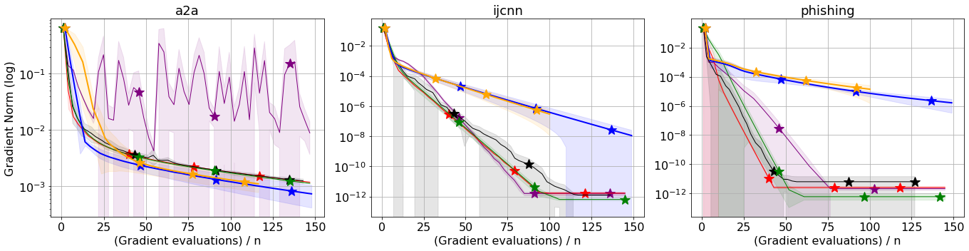
(a) Comparison against best-tuned variants

(b) Sensitivity to step-size

Figure 5: Comparison of AdaSVRG against SVRG variants, SVRG-BB and SARAH for logistic loss and batch-size = $64$. For the sensitivity to step-size plot to be readable, we limit the gradient norm to a maximum value of 10.

(a) Comparison against best-tuned variants

(b) Sensitivity to step-size

Figure 6: Comparison of AdaSVRG against SVRG variants, SVRG-BB and SARAH for Huber loss and batch-size = $64$. For the sensitivity to step-size plot to be readable, we limit the gradient norm to a maximum value of 10.

(a) Comparison against best-tuned variants

(b) Sensitivity to step-size

Figure 7: Comparison of AdaSVRG against SVRG variants, SVRG-BB and SARAH for squared loss and batch-size = $64$. For the sensitivity to step-size plot to be readable, we limit the gradient norm to a maximum value of 10. In some cases, SVRG-BB diverged, and we remove the curves accordingly so as not to clutter the plots.

L.3 Studying the effect of the batch-size on the performance of AdaSVRG

(a) Batch-size = 128

(b) Batch-size = 8

(c) Batch-size = 1

Figure 8: Comparison of AdaSVRG against best-tuned variants of SVRG, SVRG-BB and SARAH for logistic loss for different batch-sizes.

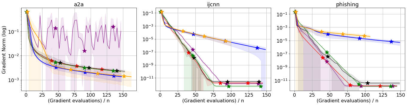
(a) Batch-size = 128

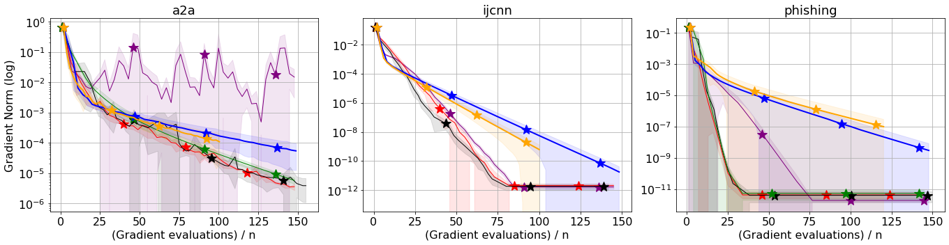
(b) Batch-size = 8

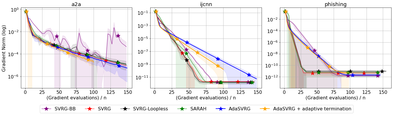
(c) Batch-size = 1

Figure 9: Comparison of AdaSVRG against best-tuned variants of SVRG, SVRG-BB and SARAH for logistic loss for different batch-sizes.

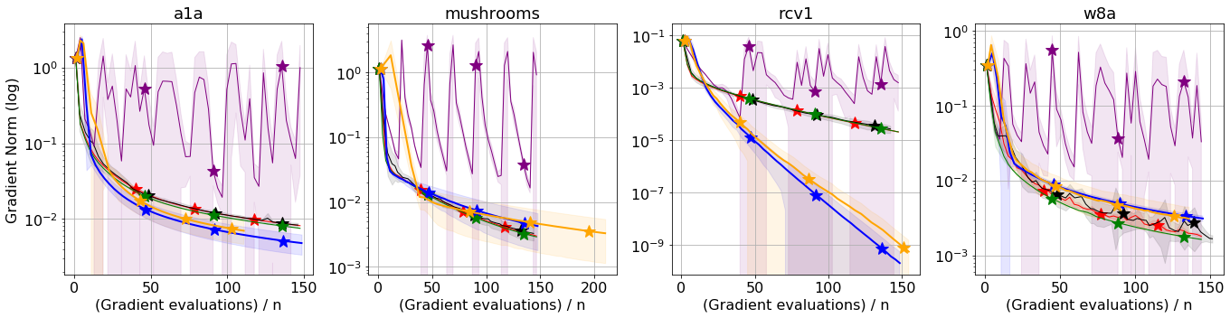
(a) Batch-size = 128

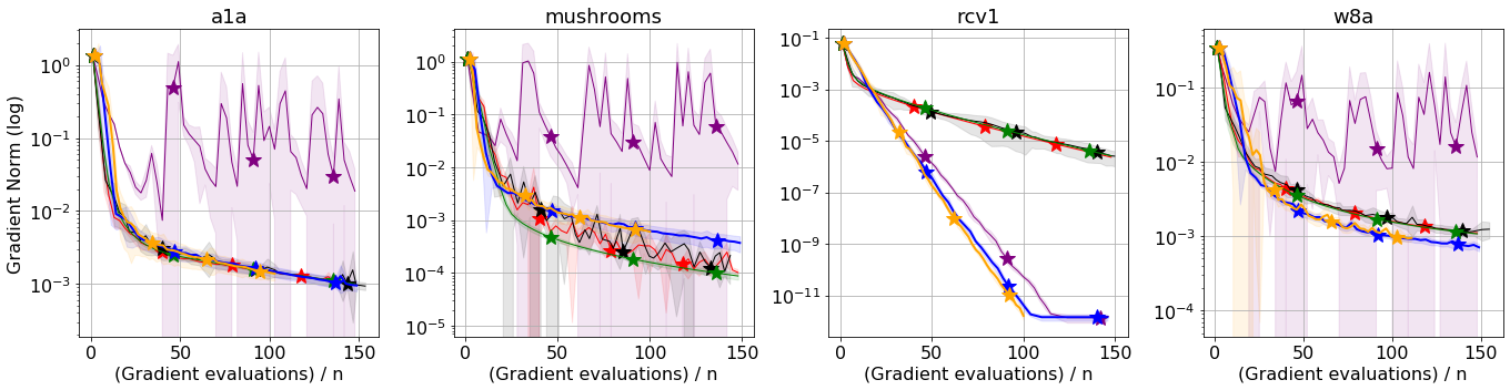
(b) Batch-size = 8

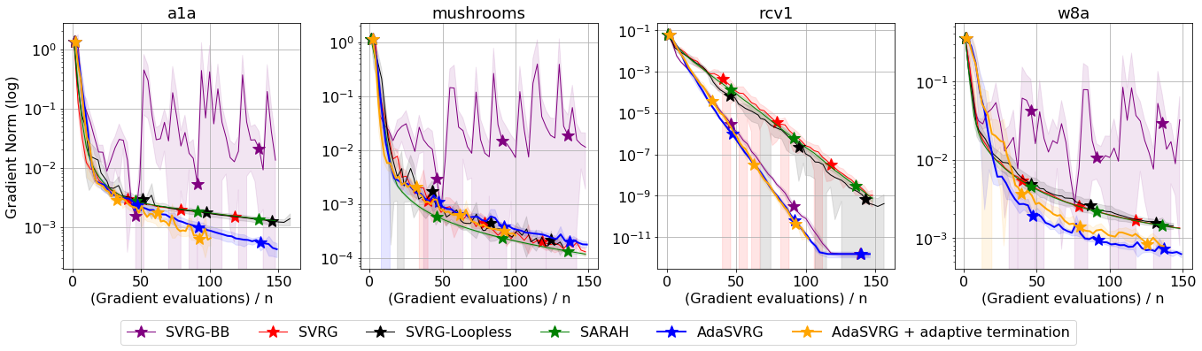
(c) Batch-size = 1

Figure 10: Comparison of AdaSVRG against best-tuned variants of SVRG, SVRG-BB and SARAH for Huber loss for different batch-sizes.

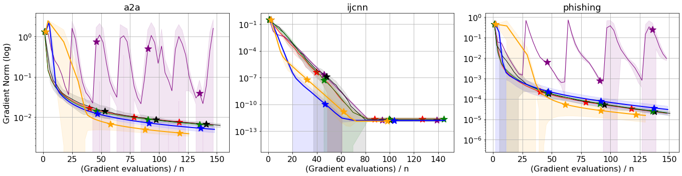
(a) Batch-size = 128

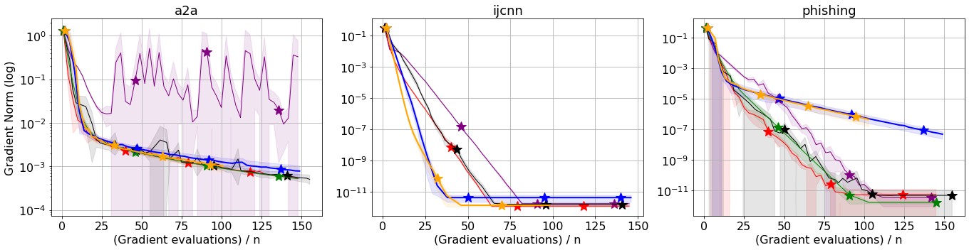
(b) Batch-size = 8

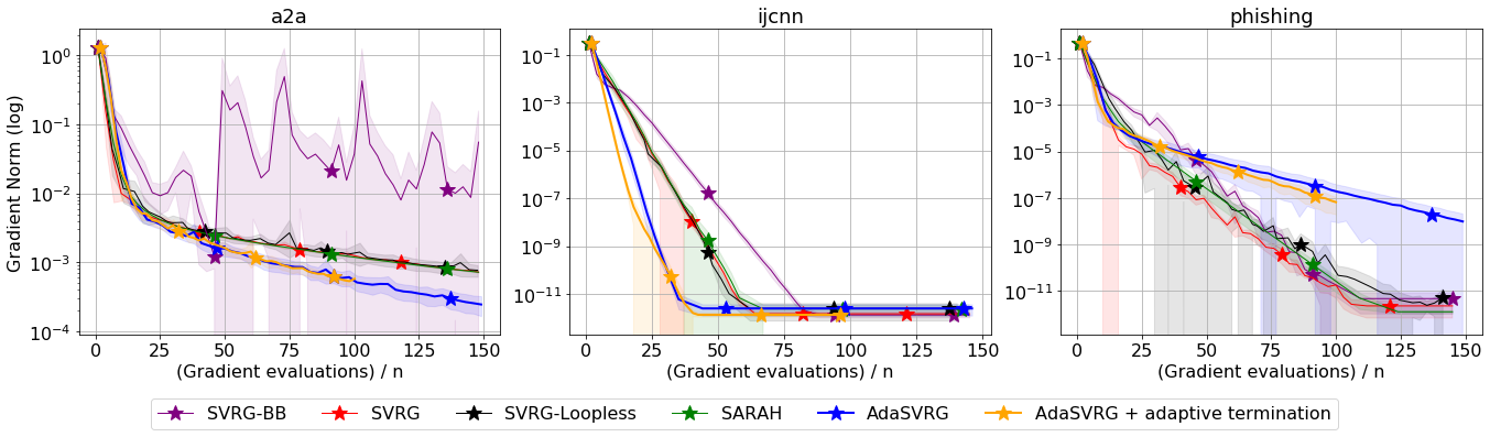
(c) Batch-size = 1

Figure 11: Comparison of AdaSVRG against best-tuned variants of SVRG, SVRG-BB and SARAH for Huber loss for different batch-sizes.

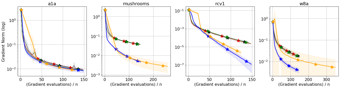
(a) Batch-size = 128

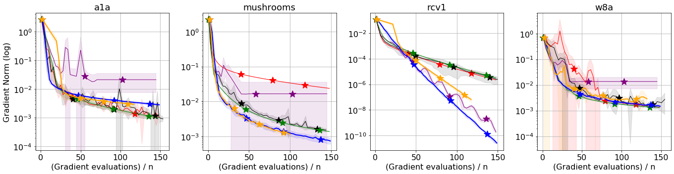
(b) Batch-size = 8

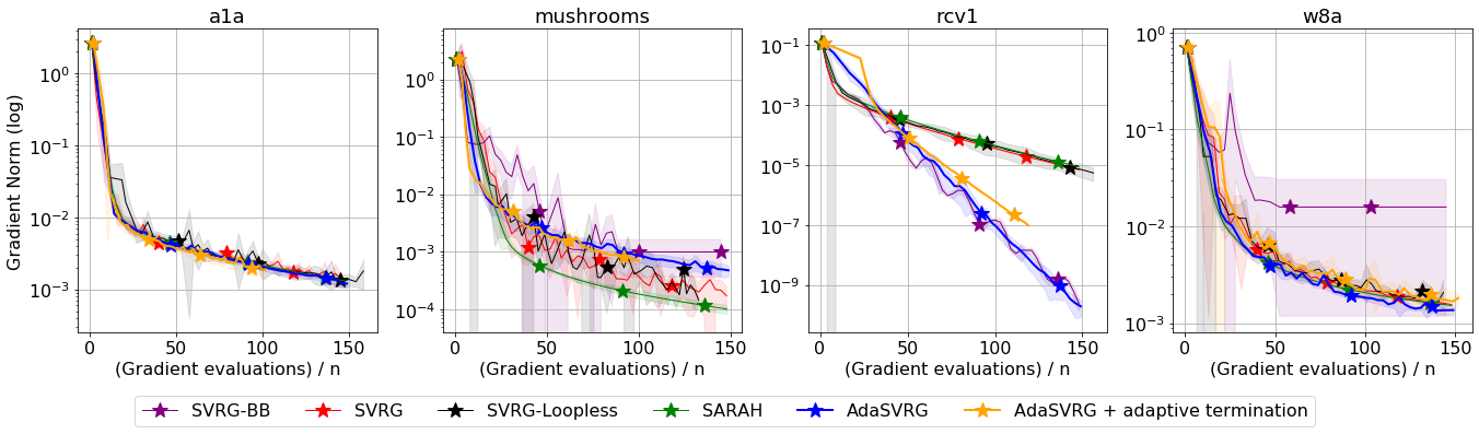
(c) Batch-size = 1

Figure 12: Comparison of AdaSVRG against best-tuned variants of SVRG, SVRG-BB and SARAH for squared loss for different batch-sizes. In some cases, SVRG-BB diverged, and we remove the curves accordingly so as not to clutter the plots.

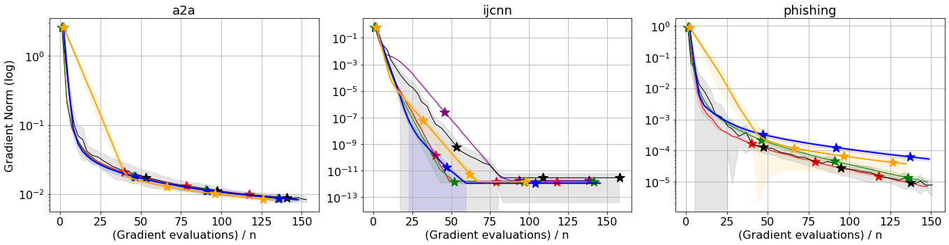
(a) Batch-size = 128

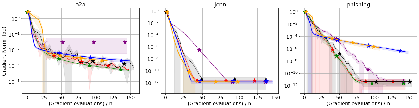
(b) Batch-size = 8

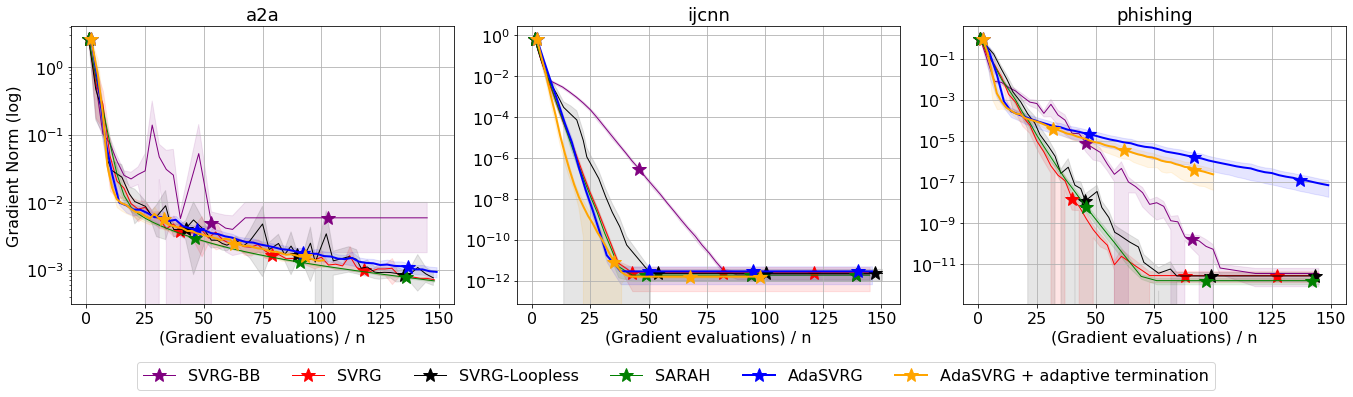
(c) Batch-size = 1

Figure 13: Comparison of AdaSVRG against best-tuned variants of SVRG, SVRG-BB and SARAH for squared loss for different batch-sizes. In some cases, SVRG-BB diverged, and we remove the curves accordingly so as not to clutter the plots.

L.4 Additional interpolation experiments

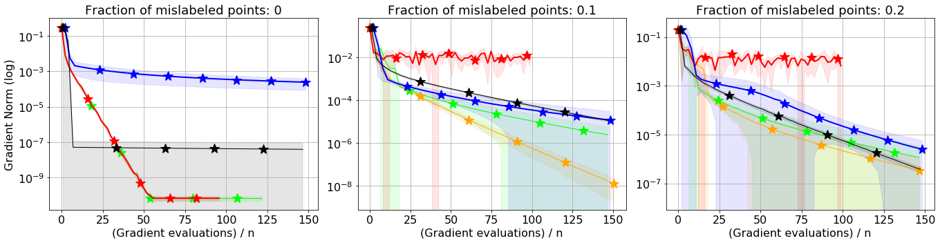
(a) Batch-size = 128

(b) Batch-size = 8

(c) Batch-size = 1

Figure 14: Comparison of best-tuned SGD, best-tuned SVRG, AdaGrad, AdaSVRG and Algorithm 4 with logisitic loss on datasets with different fraction of mislabeled data-points for different batch-sizes. Interpolation is exactly satisfied for the left-most plots.

(a) Batch-size = 128

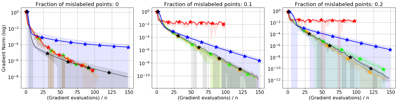
(b) Batch-size = 64

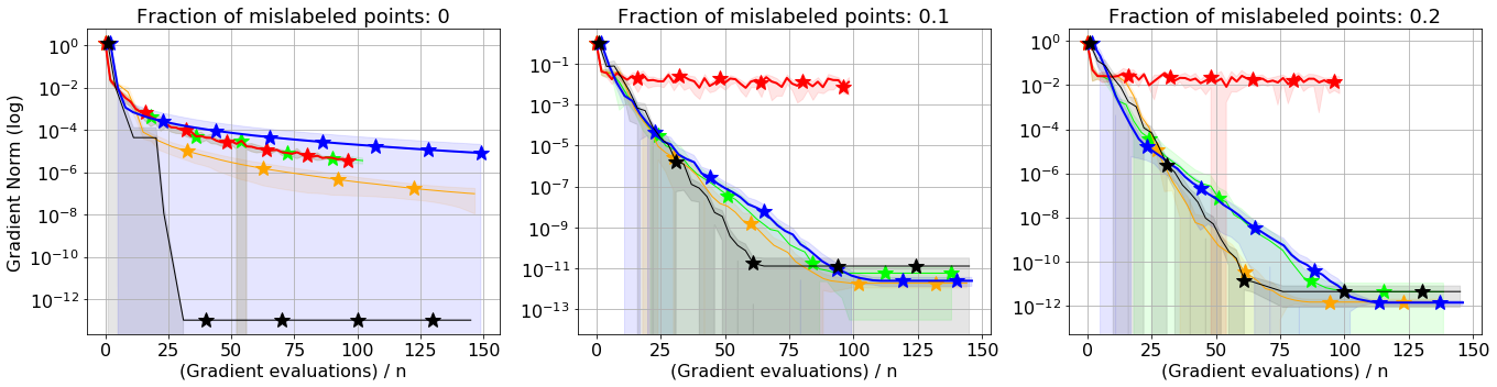
(c) Batch-size = 8

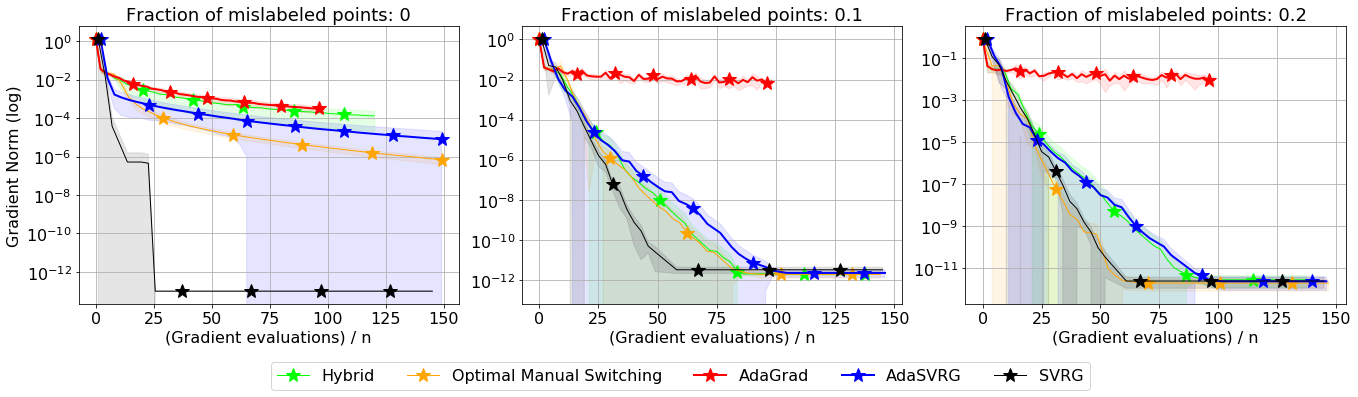
(d) Batch-size = 1

Figure 15: Comparison of best-tuned SGD, best-tuned SVRG, AdaGrad, AdaSVRG and Algorithm 4 with squared hinge loss on datasets with different fraction of mislabeled data-points for different batch-sizes. Interpolation is exactly satisfied for the left-most plots.

References

- Ahn et al., (2020) Ahn, K., Yun, C., and Sra, S. (2020). SGD with shuffling: optimal rates without component convexity and large epoch requirements. In Neural Information Processing Systems 2020, NeurIPS 2020.
- Allen-Zhu, (2017) Allen-Zhu, Z. (2017). Katyusha: The first direct acceleration of stochastic gradient methods. In Proceedings of the 49th Annual ACM SIGACT Symposium on Theory of Computing, STOC.
- Armijo, (1966) Armijo, L. (1966). Minimization of functions having lipschitz continuous first partial derivatives. Pacific Journal of mathematics, 16(1):1–3.
- Babanezhad Harikandeh et al., (2015) Babanezhad Harikandeh, R., Ahmed, M. O., Virani, A., Schmidt, M., Konečnỳ, J., and Sallinen, S. (2015). Stop wasting my gradients: Practical SVRG. Advances in Neural Information Processing Systems, 28:2251–2259.
- Barzilai and Borwein, (1988) Barzilai, J. and Borwein, J. M. (1988). Two-point step size gradient methods. IMA journal of numerical analysis, 8(1):141–148.
- Belkin et al., (2019) Belkin, M., Rakhlin, A., and Tsybakov, A. B. (2019). Does data interpolation contradict statistical optimality? In The 22nd International Conference on Artificial Intelligence and Statistics, pages 1611–1619. PMLR.
- Bollapragada et al., (2019) Bollapragada, R., Byrd, R. H., and Nocedal, J. (2019). Exact and inexact subsampled newton methods for optimization. IMA Journal of Numerical Analysis, 39(2):545–578.
- Boucheron et al., (2005) Boucheron, S., Bousquet, O., and Lugosi, G. (2005). Theory of classification: A survey of some recent advances. ESAIM: probability and statistics, 9:323–375.
- Chang and Lin, (2011) Chang, C.-C. and Lin, C.-J. (2011). LIBSVM: A library for support vector machines. ACM Transactions on Intelligent Systems and Technology, 2(3):1–27. Software available at http://www.csie.ntu.edu.tw/~cjlin/libsvm.
- Cutkosky and Boahen, (2017) Cutkosky, A. and Boahen, K. (2017). Online convex optimization with unconstrained domains and losses. arXiv preprint arXiv:1703.02622.
- Cutkosky and Orabona, (2019) Cutkosky, A. and Orabona, F. (2019). Momentum-based variance reduction in non-convex SGD. arXiv preprint arXiv:1905.10018.
- Defazio et al., (2014) Defazio, A., Bach, F., and Lacoste-Julien, S. (2014). SAGA: A fast incremental gradient method with support for non-strongly convex composite objectives. In Advances in Neural Information Processing Systems, NeurIPS.
- Defazio and Bottou, (2019) Defazio, A. and Bottou, L. (2019). On the ineffectiveness of variance reduced optimization for deep learning. In Advances in Neural Information Processing Systems, NeurIPS.
- Duchi et al., (2011) Duchi, J. C., Hazan, E., and Singer, Y. (2011). Adaptive subgradient methods for online learning and stochastic optimization. The Journal of Machine Learning Research, 12:2121–2159.
- Gower et al., (2020) Gower, R. M., Schmidt, M., Bach, F., and Richtarik, P. (2020). Variance-reduced methods for machine learning. Proceedings of the IEEE, 108(11):1968–1983.
- Hofmann et al., (2015) Hofmann, T., Lucchi, A., Lacoste-Julien, S., and McWilliams, B. (2015). Variance reduced stochastic gradient descent with neighbors. Advances in Neural Information Processing Systems, 28:2305–2313.
- Johnson and Zhang, (2013) Johnson, R. and Zhang, T. (2013). Accelerating stochastic gradient descent using predictive variance reduction. In Advances in Neural Information Processing Systems, NeurIPS.
- Konečnỳ and Richtárik, (2013) Konečnỳ, J. and Richtárik, P. (2013). Semi-stochastic gradient descent methods. arXiv preprint arXiv:1312.1666.
- Kovalev et al., (2020) Kovalev, D., Horváth, S., and Richtárik, P. (2020). Don’t jump through hoops and remove those loops: SVRG and Katyusha are better without the outer loop. In Algorithmic Learning Theory, pages 451–467. PMLR.
- Lan et al., (2019) Lan, G., Li, Z., and Zhou, Y. (2019). A unified variance-reduced accelerated gradient method for convex optimization. In Advances in Neural Information Processing Systems, pages 10462–10472.
- Lang et al., (2019) Lang, H., Xiao, L., and Zhang, P. (2019). Using statistics to automate stochastic optimization. In Advances in Neural Information Processing Systems, pages 9540–9550.
- Levy et al., (2018) Levy, K. Y., Yurtsever, A., and Cevher, V. (2018). Online adaptive methods, universality and acceleration. In Advances in Neural Information Processing Systems, NeurIPS.
- Li et al., (2020) Li, B., Wang, L., and Giannakis, G. B. (2020). Almost tune-free variance reduction. In International Conference on Machine Learning, pages 5969–5978. PMLR.
- Liang et al., (2020) Liang, T., Rakhlin, A., et al. (2020). Just interpolate: Kernel “ridgeless” regression can generalize. Annals of Statistics, 48(3):1329–1347.
- Liu et al., (2020) Liu, M., Zhang, W., Orabona, F., and Yang, T. (2020). Adam+: A stochastic method with adaptive variance reduction. arXiv preprint arXiv:2011.11985.
- Loizou et al., (2020) Loizou, N., Vaswani, S., Laradji, I., and Lacoste-Julien, S. (2020). Stochastic Polyak step-size for SGD: An adaptive learning rate for fast convergence. arXiv preprint:2002.10542.
- Ma et al., (2018) Ma, S., Bassily, R., and Belkin, M. (2018). The power of interpolation: Understanding the effectiveness of SGD in modern over-parametrized learning. In Proceedings of the 35th International Conference on Machine Learning, ICML.
- Mahdavi and Jin, (2013) Mahdavi, M. and Jin, R. (2013). MixedGrad: An O(1/T) convergence rate algorithm for stochastic smooth optimization. arXiv preprint arXiv:1307.7192.
- Mairal, (2013) Mairal, J. (2013). Optimization with first-order surrogate functions. In International Conference on Machine Learning, pages 783–791.
- Meng et al., (2020) Meng, S. Y., Vaswani, S., Laradji, I., Schmidt, M., and Lacoste-Julien, S. (2020). Fast and furious convergence: Stochastic second order methods under interpolation. In The 23nd International Conference on Artificial Intelligence and Statistics, AISTATS.
- Nesterov, (2004) Nesterov, Y. (2004). Introductory lectures on convex optimization: A basic course. Springer Science & Business Media.
- Nguyen et al., (2017) Nguyen, L. M., Liu, J., Scheinberg, K., and Takáč, M. (2017). SARAH: a novel method for machine learning problems using stochastic recursive gradient. In Proceedings of the 34th International Conference on Machine Learning-Volume 70, pages 2613–2621.
- Pesme et al., (2020) Pesme, S., Dieuleveut, A., and Flammarion, N. (2020). On convergence-diagnostic based step sizes for stochastic gradient descent. arXiv preprint arXiv:2007.00534.
- Pflug, (1983) Pflug, G. C. (1983). On the determination of the step size in stochastic quasigradient methods.
- Qian and Qian, (2019) Qian, Q. and Qian, X. (2019). The implicit bias of adagrad on separable data. arXiv preprint arXiv:1906.03559.
- Reddi et al., (2016) Reddi, S. J., Hefny, A., Sra, S., Poczos, B., and Smola, A. (2016). Stochastic variance reduction for nonconvex optimization. In International conference on machine learning, pages 314–323.
- Reddi et al., (2018) Reddi, S. J., Kale, S., and Kumar, S. (2018). On the convergence of Adam and Beyond. In International Conference on Learning Representations.
- Schmidt et al., (2015) Schmidt, M., Babanezhad, R., Ahmed, M., Defazio, A., Clifton, A., and Sarkar, A. (2015). Non-uniform stochastic average gradient method for training conditional random fields. In Proceedings of the Eighteenth International Conference on Artificial Intelligence and Statistics, AISTATS.
- Schmidt and Le Roux, (2013) Schmidt, M. and Le Roux, N. (2013). Fast convergence of stochastic gradient descent under a strong growth condition. arXiv preprint:1308.6370.
- Schmidt et al., (2017) Schmidt, M., Le Roux, N., and Bach, F. (2017). Minimizing finite sums with the stochastic average gradient. Mathematical Programming, 162(1-2):83–112.
- Sebbouh et al., (2019) Sebbouh, O., Gazagnadou, N., Jelassi, S., Bach, F., and Gower, R. (2019). Towards closing the gap between the theory and practice of SVRG. In Advances in Neural Information Processing Systems, pages 648–658.
- Shalev-Shwartz and Zhang, (2013) Shalev-Shwartz, S. and Zhang, T. (2013). Stochastic dual coordinate ascent methods for regularized loss minimization. Journal of Machine Learning Research, 14(Feb):567–599.
- Song et al., (2020) Song, C., Jiang, Y., and Ma, Y. (2020). Variance reduction via accelerated dual averaging for finite-sum optimization. Advances in Neural Information Processing Systems, 33.
- Sridharan et al., (2008) Sridharan, K., Shalev-Shwartz, S., and Srebro, N. (2008). Fast rates for regularized objectives. Advances in neural information processing systems, 21:1545–1552.
- Tan et al., (2016) Tan, C., Ma, S., Dai, Y.-H., and Qian, Y. (2016). Barzilai-Borwein step size for stochastic gradient descent. arXiv preprint arXiv:1605.04131.
- (46) Vaswani, S., Bach, F., and Schmidt, M. (2019a). Fast and faster convergence of SGD for over-parameterized models and an accelerated perceptron. In The 22nd International Conference on Artificial Intelligence and Statistics, AISTATS.
- Vaswani et al., (2020) Vaswani, S., Kunstner, F., Laradji, I., Meng, S. Y., Schmidt, M., and Lacoste-Julien, S. (2020). Adaptive gradient methods converge faster with over-parameterization (and you can do a line-search). arXiv preprint arXiv:2006.06835.
- (48) Vaswani, S., Mishkin, A., Laradji, I., Schmidt, M., Gidel, G., and Lacoste-Julien, S. (2019b). Painless stochastic gradient: Interpolation, line-search, and convergence rates. In Advances in Neural Information Processing Systems, NeurIPS.
- Ward et al., (2019) Ward, R., Wu, X., and Bottou, L. (2019). AdaGrad stepsizes: Sharp convergence over nonconvex landscapes, from any initialization. In Proceedings of the 36th International Conference on Machine Learning, ICML.
- Yaida, (2018) Yaida, S. (2018). Fluctuation-dissipation relations for stochastic gradient descent. arXiv preprint arXiv:1810.00004.
- Zhang et al., (2017) Zhang, C., Bengio, S., Hardt, M., Recht, B., and Vinyals, O. (2017). Understanding deep learning requires rethinking generalization. In 5th International Conference on Learning Representations, ICLR.