e1e-mail: capozziello@unina.it \thankstexte2e-mail: mirfaizalmir@googlemail.com \thankstexte3e-mail: hme123eda@gmail.com \thankstexte4e-mail: b.pourhassan@du.ac.ir \thankstexte5e-mail: vincenzo.salzano@usz.edu.pl
Logarithmic corrections to Newtonian gravity and Large Scale Structure
Abstract
Effects from nonstandard corrections to Newtonian gravity, at large scale, can be investigated using the cosmological structure formation. In particular, it is possible to show if and how a logarithmic correction (as that induced from nonlocal gravity) modifies the clustering properties of galaxies and of clusters of galaxies. The thermodynamics of such systems can be used to obtain important information about the effects of such modification on clustering. We will compare its effects with observational data and it will be demonstrated that the observations seem to point to a characteristic scale where such a logarithmic correction might be in play at galactic scales. However, at larger scales such statistical inferences are much weaker, so that a fully reliable statistical evidence for this kind of corrections cannot be stated without further investigations and the use of more varied and precise cosmological and astrophysical probes.
1 Introduction
The clustering of galaxies is the main mechanism to address the large scale structure of the Universe. Such clustering mechanism can be studied confronting numerical simulations (Frenk et al., 1999; Barnes et al., 2017) with observations (Ponman et al., 2003; Voit, 2005), using the local matter distributions of galaxies organized in groups, filaments and clusters. However, to analyze numerically the large scale structure formation, it is possible to approximate galaxies as point-like particles, and then study the clustering adopting the standard formalism of statistical mechanics. This approximation is valid because the distance between galaxies is much larger than their proper size. In fact, it has been demonstrated that the clustering mechanism can be studied considering a quasi-equilibrium description because the macroscopic quantities change very slowly as compared with the local relaxation time scales (Saslaw and Yang, 2009; Saslaw and Fang, 1996; Saslaw and Sheth, 1993; Rahmani et al., 2009). Pressure, average density and average temperature of clusters are the macroscopic quantities to be taken into account. Here the temperature is the effective one obtained by the kinetic theory of gases, for a gas of galaxies (each galaxy being approximated as a point particle). So, by this quasi-equilibrium description, the clustering of galaxies can be dealt as a thermodynamic system (Itoh et al., 1993; Saslaw et al., 1990). Specifically, one has to adopt a gravitational partition function (Saslaw, 1986; Saslaw et al., 1990) where point-like galaxies gravitationally interact. Such a partition function can be also used to study phase transitions for systems of interacting galaxies (Saslaw and Ahmad, 2010; Upadhyay et al., 2018; Khan and Malik, 2012).
It has to be pointed out that such a gravitational partition function diverges because the extended structure of galaxies has been neglected in this approximation. However, these divergences can be removed by adding a softening parameter, which accounts for the extended structure of galaxies as reported in (Ahmad and Hameeda, 2010). In a recent study it has also been proved that the nonlocal gravity is divergence free Hameeda et al. (2021). Thermodynamics for systems of galaxies is obtained from the partition function (regularized with a softening parameter), and this can in turn be used to study the clustering properties (Saslaw and Hamilton, 1984). It has been observed that any modification of gravitational partition function by a softening parameter, in turn, modifies the thermodynamic quantities of a given system. Vice versa, because these thermodynamic quantities are related to the clustering parameter, it also changes the clustering parameter itself. In fact, it can be demonstrated that the modification to the skewness and kurtosis of clustering systems occur due to such a softening parameter (Ahmad et al., 2002). This formalism has also been used to demonstrated that galaxy clusters are surrounded by halos, and this has been done adopting a wide range of samples (Sivakoff and Saslaw, 2005; Rahmani et al., 2009). Furthermore the isothermal compressibility gives also information on the clustering of galaxies (Ahmad et al., 2006).
Specifically, the clustering of galaxies occurs due to the gravitational force between them. However, it is now well-known by a wide range of cosmological observations (e.g. Type Ia Supernovae, Baryon Acoustic Oscillations and Cosmic Microwave Background) that the Universe is undergoing an accelerating expansion (Riess et al., 1998; Perlmutter et al., 1999; Aghanim et al., 2020). This cosmic expansion is pulling the galaxies away from each other. So, the cosmic expansion seems to oppose the gravitational force, and thus it is important to include its effect in the gravitational partition function. It has been argued that the cosmological constant related to the accelerated expansion can produce important local effects on the scale of galaxy clusters (Gurzadyan et al., 2020; Gurzadyan and Stepanian, 2018, 2019a; Gurzadyan and Penrose, 2013; Gurzadyan and Stepanian, 2019b). These effects can be investigated using model of interacting dark matter and dark energy (Gurzadyan et al., 2020; Gurzadyan and Stepanian, 2018). It is also possible to constrain the dark energy from the clustering of galaxies (Le Delliou et al., 2019). The cosmic expansion can also change the dynamics at the scale of galaxy clusters (Boonserm et al., 2020). Such a modification of cluster dynamics has also been investigated using different groups of galaxies (Peirani and Pacheco, 2008). Finally, one can state that the cosmological constant has consequences for the formation of galaxy clusters (Iliev and Shapiro, 2001). In summary, it is important to study the effects of cosmic expansion at the scale of clusters. From a more technical point of view, it has to be noted that the Fisher matrix formalism has been used to analyze the effects of cosmic expansion on clusters (Stark et al., 2017).
Thus, it is possible to obtain information about the cosmological constant, and, in general, about dark energy dynamics, from the local clustering of galaxies. So, it is important to incorporate the effects of cosmic expansion in the statistical mechanical description of the clustering of galaxies. In fact, an accurate measurement of the statistics of galaxies can be used to constraint the value of the cosmological constant (Aguena and Lima, 2018), and the distribution function of galaxies can be used to constraint the amount of the dark energy (Wen et al., 2020).
As such a statistical distribution function can be obtained from the gravitational partition function (Itoh et al., 1993; Saslaw et al., 1990), it is important to incorporate the effects of cosmic expansion in the partition function. So, the modification of the gravitational partition function by the cosmological constant term has also to be considered, and this modified gravitational partition function can be used to study the clustering process in an expanding Universe (Hameeda et al., 2016). This can be technically done by first analyzing the Helmholtz free energy and entropy for a system of galaxies. Then the clustering parameter for this system can be obtained, and it has been observed that this clustering parameter depends on the value of the cosmological constant. The modification of the gravitational partition function with a time dependent cosmological constant can be also used to study the effects of dynamical dark energy on clustering of galaxies (Pourhassan et al., 2017). It has been observed that the correlation function for this system are consistent with observations.
However, it is possible to obtain cosmic expansion without considering dark energy related to some new fundamental particle. In fact, large scale nonlocality related to some effective gravitational potential seems a realistic effect of gravitational field at infrared scales as recently reported in several papers, see for example (Deser and Woodard, 2007; Ding and Deng, 2019; Bahamonde et al., 2017a, b; Bajardi et al., 2020). It has been argued that such nonlocalities can occur due to some quantum gravitational effects (Deser and Woodard, 2007; Ding and Deng, 2019; Modesto and Rachwał, 2017). They can be relevant also in gravitational waves modes and polarizations (Capozziello et al., 2020; Belgacem et al., 2019). It has been demonstrated that string field theory produces nonlocal actions for the component fields, and these nonlocal actions can also be used to construct nonlocal cosmological models (Koshelev, 2007; Koshelev and Vernov, 2012). It is also possible to construct models of nonlocal cosmology from loop quantum gravity (Gielen et al., 2013; Gielen, 2019). This can be done adopting a sort of condensation of states in loop quantum gravity. In summary, it is possible to obtain nonlocal cosmologies using quantum gravitational effects at ultraviolet scales that propagate up to infrared scales.
In other words, as nonlocal cosmology can explain the cosmic expansion without dark energy (Deser and Woodard, 2007; Ding and Deng, 2019; Bahamonde et al., 2017a, b; Bajardi et al., 2020), such nonlocal corrections can also be used to incorporate the effects of cosmic expansion in the gravitational partition function. This one can then be used to analyze the effects of nonlocality on clustering of galaxies. It may be noted that even though general relativity is strongly constrained at the Solar System scales by several experiments and observations (Yunes and Siemens, 2013; Chicone and Mashhoon, 2016a; Tian and Zhu, 2019), nonlocal modification to general relativity can occur at large scales starting from galactic one (Dialektopoulos et al., 2019). At the same time, nonlocal gravity is safe from possible issues related to oscillating features on small scales, falling in the regime where such oscillations are subdominant Lazar (2020). It has also been proposed that such nonlocality could be constrained from the clustering of galaxies (Amendola et al., 2019). Thus, it is important to analyze the effect of nonlocal modification of gravity on the gravitational partition function and point out how it affects the clustering process. Such a modification can be analyzed using nonlocal corrections to the gravitational potential (Dialektopoulos et al., 2019; Hehl and Mashhoon, 2009a, b; Blome et al., 2010; Chicone and Mashhoon, 2016b). In general, the nonlocal gravitational partition function can be used to analyze the effects of nonlocality on clustering of galaxies. Although our main motivation for such a study is related to testing nonlocal gravity, we must note here that the logarithmic correction induced by such a theory is shared also by other alternative models of gravity, e.g. MOND (Shapiro et al., 2005; Famaey and McGaugh, 2012), Randall-Sundrum brane scenario (Park and Tamaryan, 2003), or other string-theoretical motivations (Soleng, 1995) which have been also tested with internal dynamics of spiral galaxies (Fabris and Campos, 2009). It may be noted that there is an intrinsic non-locality in string theory (Calcagni and Modesto, 2014; Biswas et al., 2012). Furthermore, even MOND has been related to nonlocality (Soussa and Woodard, 2003; Deffayet et al., 2011, 2014; Tan and Woodard, 2018; Kim et al., 2016). This could be due to the fact that nonlocality (Deser and Woodard, 2007; Ding and Deng, 2019), and several of these modifications, are motivated from quantum corrections to the original Einstein-Hilbert action. Even MOND can be obtained as a quantum correction in the Verlinde formalism (Bagchi and Fring, 2019). Thus, we expect some kind of universal form of correction to occur in most of them. In this perspective, our results will be more general and not strictly related to one particular scenario.
In Sec. 2, we discuss the clustering mechanism. After defining the nonlocal gravitational partition function, we consider the related thermodynamics and spatial correlation function. Observational data analysis is described in detail in Sec. 3. Specifically, we take into account data from galaxies and clusters and study the effects of nonlocality on the clustering mechanism. Results are discussed in Sec. 4, while conclusions are drawn in Sec. 5.
2 Modeling Clusters of galaxies
In general, a nonlocal modification of the Hilbert-Einstein action can have the following form (Deser and Woodard, 2007; Ding and Deng, 2019)
| (1) |
where is the Ricci scalar and is an arbitrary function, called distortion function, of the nonlocal term , which is explicitly given by the retarder Green’s function
| (2) |
Setting , the above action is equivalent to the Einstein-Hilbert one. The nonlocality is introduced by the inverse of the d’Alembert operator. In order to "localize" the action, an auxiliary scalar field can be introduced so that and then formally . As a consequence, characteristic lengths related to the nonlocal terms naturally come out (Dialektopoulos et al., 2019).
The weak-field limit of such a dynamics gives rise to corrections to the Newtonian potential which are interesting at large scales. These corrections can be polynomial or logarithmic and, in general, introduce characteristic scales. For a detailed discussion on this point see (Dialektopoulos et al., 2019).
In the framework of this theory, let us now model the clustering of galaxies using the gravitational partition function which we are going to define. We will explicitly adopt the nonlocal gravity, as discussed in (Hehl and Mashhoon, 2009b; Blome et al., 2010; Chicone and Mashhoon, 2016b), to obtain the corrections to such a gravitational partition function. After analyzing the effects of nonlocality, the nonlocal gravitational partition function will be used to analyze the clustering of galaxies. This can be done by considering the thermodynamics of this system, and then relating it to the clustering parameter. Then we will calculate the spatial correlation function.
2.1 Nonlocal Gravitational Partition Function
Let us take into account a system with a large number of galaxies. This system can be analyzed using a quasi-equilibrium description, where the change in macroscopic quantities is slower than the local relaxation time scales (Saslaw and Yang, 2009; Saslaw and Fang, 1996; Saslaw and Sheth, 1993; Rahmani et al., 2009). It is possible analyze such a system adopting an ensemble of cells, with same volume , or radius and average density. As the number of galaxies and their total energy can vary between these cells, the system can be analyzed in the framework of the grand canonical ensemble. Thus, it is possible to define a gravitational partition function. In this picture, a system of galaxies of mass interacting with a nonlocal gravitational potential can be written as (Saslaw, 1986; Saslaw et al., 1990)
| (3) | |||||
where are the momenta of different galaxies and is the nonlocal gravitational potential energy. Here is the average temperature, which is obtained from the kinetic theory of gases where each particle is represented by a galaxy. Now integrating on the momentum space, we can write this gravitational partition function as
| (4) |
where , the configuration integral, can be expressed as
| (5) |
The nonlocal gravitational potential energy is a function of the relative position vector , as both the local and nonlocal terms represent central forces. The total potential energy can be obtained by summing up the potential energies. So, we can write the total nonlocal potential energy as
| (6) |
We can write such a nonlocal gravitational potential energy for galaxies as (Hehl and Mashhoon, 2009b; Blome et al., 2010; Chicone and Mashhoon, 2016b)
| (7) |
Since galaxies have an extended structure, we need to modify the gravitational potential energy by a softening parameter (Ahmad and Hameeda, 2010; Ahmad et al., 2006). Thus, we can write
| (8) |
Now we can use a nonlocal two-point interaction function for galaxies to analyze this system. It vanishes in absence of interactions, and it is non-zero only for interacting galaxies. Thus, we can now express the nonlocal configuration integral as
| (9) | |||||
where we can express the nonlocal two-point interaction Mayer function as
| (10) |
It is worth noticing that such an expression for clustering integral has been discussed for local gravitational interactions (Ahmad et al., 2002, 2006). Here we have obtained the contributions to such Mayer function from nonlocal gravitational interactions (Hehl and Mashhoon, 2009b; Blome et al., 2010; Chicone and Mashhoon, 2016b). We can expand this nonlocal two-point interaction Mayer function as a power series. So, we can write as
| (11) |
Now using , we can write as
| (12) | |||||
where is given by
| (13) |
It may be noted here that is the hypergeometric function. Now using , we observe that So, using the scale invariance, , and , we can define as
| (14) |
where . From this expression for , we can obtain any general configuration integral. Using the so called dilute approximation, we can assume very small and take only the first term of the exponential expansion,
| (15) |
Thus, calculating the general configuration integral, we obtain
| (16) |
where
Now the gravitational partition function for this dilute gravitating system can be written as
| (18) |
This expression for the gravitational partition function can be used to analyze the effects of nonlocality on the clustering of galaxies.
2.2 Thermodynamics
It has to be noted that the gravitational partition function has already been used to study the thermodynamics of systems of galaxies, see (Itoh et al., 1993) and (Saslaw et al., 1990). We can thus adopt the nonlocal gravitational partition function to analyze the thermodynamics of this nonlocal system. The Helmholtz free energy is
| (19) |
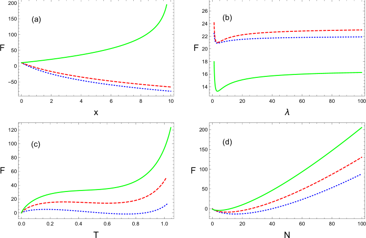
In the plots of Fig. 1, we analyze the dependence of the Helmholtz free energy on various parameters. The dependence of Helmholtz free energy on is represented in Fig. 1 (a). We can observe that the Helmholtz free energy is a decreasing function of for large value of the nonlocality parameter and an increasing function of for smaller value of the nonlocality parameter . So, the value of nonlocality parameter changes the dependence of the Helmholtz free energy on . In Fig. 1 (b), the Helmholtz free energy is plotted in terms of . We can see how there is a minimum for the Helmholtz free energy, and this minimum seems to occur at a specific value of . This minimum does not seem to change with the temperatures of the system. This observation can explain the change in the behavior of the Helmholtz free energy with the change in the value of , as was observed in Fig. 1 (a). In Fig. 1 (c), we plot the dependence of the Helmholtz free energy on the temperature of the system. Here the temperature corresponds to the temperature of a gas of galaxies, with each galaxy acting as a particle analog. We observe that generally the Helmholtz free energy increases with the temperature, but the rate of this increase depends on the number of galaxies. As we have plotted the dependence on temperature by considering the system as a gas of galaxies, we also analyze the dependence of the Helmholtz free energy on the number of galaxies in Fig. 1 (d). We observe that the Helmholtz free energy first decreases for a relatively small number of galaxies, becoming negative, and then increases as the number of galaxies becomes more than a certain value.
The entropy can now be calculated from this Helmholtz free energy, as
| (20) |
Now, for large , using , we obtain
| (21) |
where . where
| (22) |
This is the general clustering parameter for a system of galaxies interacting in presence of nonlocal gravity. The internal energy of a system of galaxies can now be written as
| (23) |
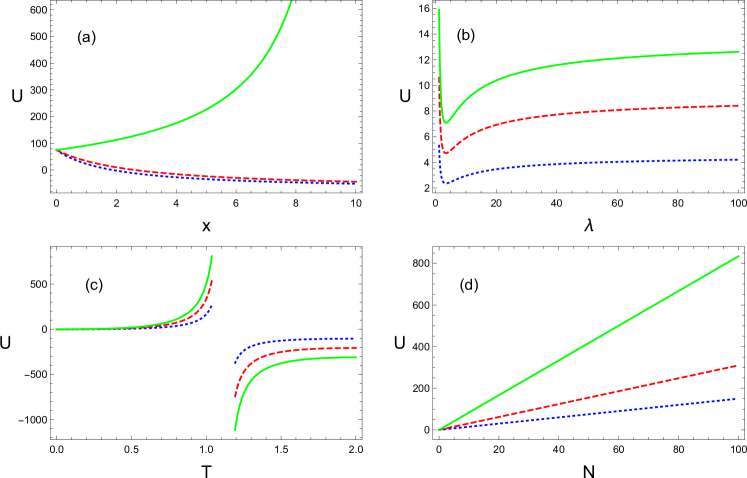
We have plotted the internal energy of a system of galaxies in Fig. 2. Its behavior is analyzed by investigating its dependence on various parameters. In Fig. 2 (a), we investigate how the internal energy of the system varies with . We observe that it is an increasing function of for smaller values of , and a decreasing function of for larger values of . In Fig. 2 (b), we analyze the dependence of the internal energy on the nonlocality parameter . We observe that there is a minimum for internal energy, and again this minimum does not seem to depend on the temperature of the system. We also investigate the dependence of the internal energy on the temperate of the system in Fig. 2 (c). It is observed that there is a discontinuity in the dependence of internal energy on temperature, which occurs independently of the number of galaxies. In Fig. 2 (d), the dependence of internal energy on the number of galaxies is plotted. It is observed that internal energy increases with the increase in the number of galaxies. However, the rate of increase is larger for larger values of .
Similarly, we can write the pressure and chemical potential for galaxies interacting through a nonlocal gravitational potential as
| (24) | ||||
The probability of finding galaxies can be written as
| (25) |
where is the grand-partition function defined by
| (26) |
and is the activity. Thus, for a system of gravitationally interacting galaxies in nonlocal gravity , we can write
| (27) |
Now the grand-partition function can be written as
| (28) |
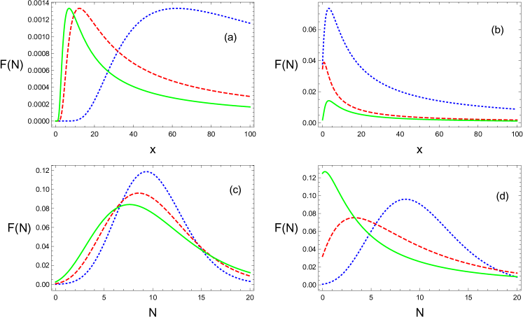
and the distribution function can be expressed as
| (29) |
In Fig. 3, we analyze the behavior of the distribution function for galaxies, and its dependence on different parameters used here. In general, the distribution function has the universal feature of having a maximum, while its functional shape changes, and depends on the considered parameters.
2.3 Spatial correlation function
It is well know that the interaction between different galaxies will cause correlation in their positions. The integral of the correlation function over a certain volume can be expressed in terms of the mean square fluctuation of the total number of galaxies in a given volume. Thus we can write
| (30) |
This can be further represented in terms of thermodynamic quantities as
| (31) |
Taking the volume derivative and using the equation of state for pressure , we get
| (32) |
The pressure can be written in terms of the clustering parameter as
| (33) |
We can write the change of volume with pressure at constant temperature
| (34) |
The expression for is
| (35) |
where and . Now we can write
| (36) |
The volume integral of correlation function is the quantity which can be compared with observational data in order to detect possible effects of nonlocal gravity.
3 Observational Data Analysis
We will test the nonlocal gravitational clustering with the cluster catalog in (Wen et al., 2012), containing clusters of galaxies in the redshift range from the Sloan Digital Sky Survey III (SDSS-III). We will take advantage of this catalog because it has all the needed ingredients to analyze clustering properties of both galaxies and clusters (although an alternative more recent version is in Wen and Han (2015)), using two different approaches.
3.1 Galaxies
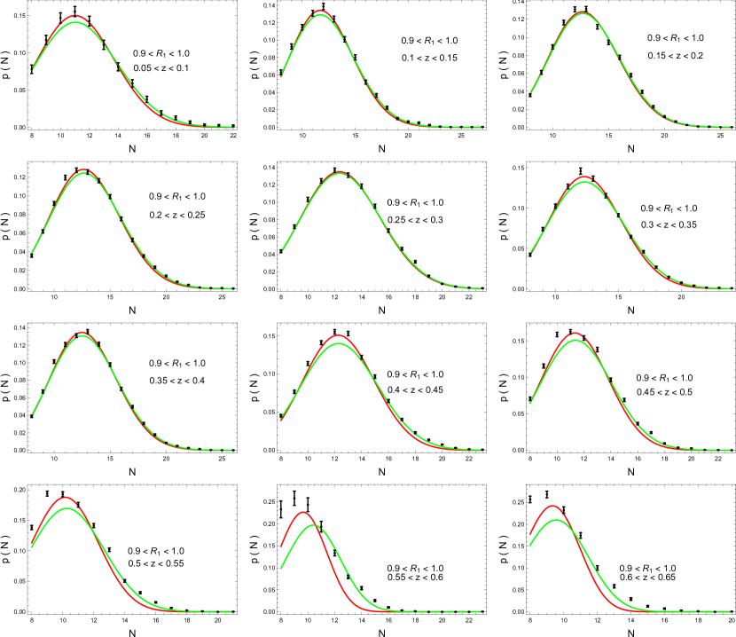
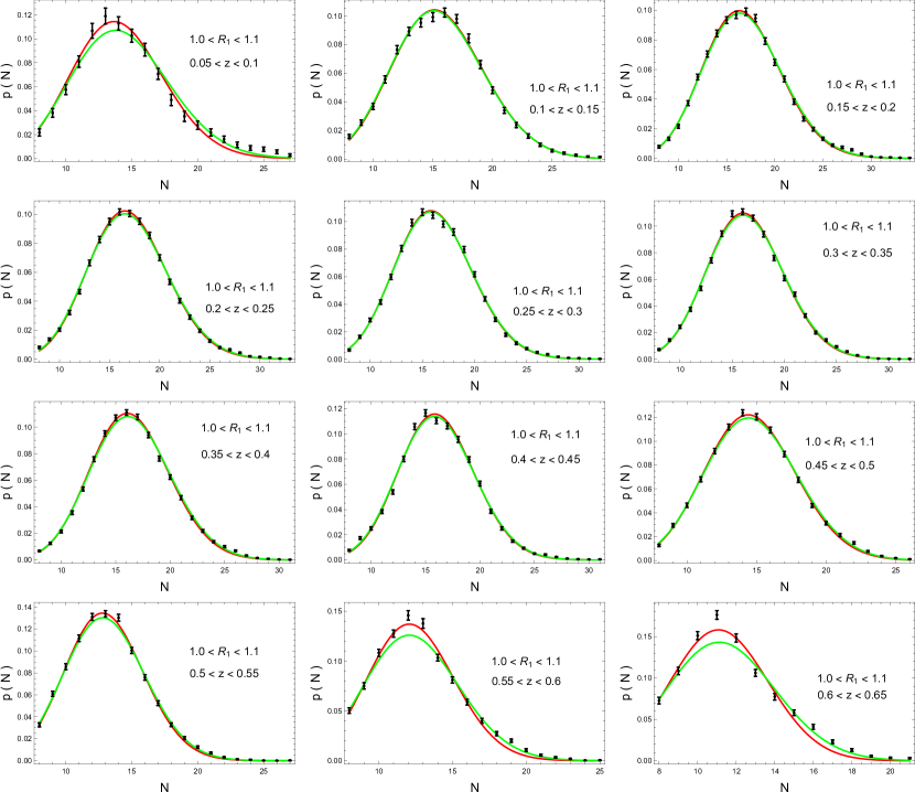
The analysis of the clustering of galaxies will be conducted with a sort of “smart” version of the standard counts-in-cell procedure. In general, one would first need to define cells/volumes with a given size, and then to count the gravitational structures of interest within them. Here, our “smart” volumes will be the clusters identified in the SDSS-III survey, and we will count the galaxies which are within each of them. From this procedure, we will be able to calculate the observed distribution function and to compare it with the theoretical expectation in nonlocal gravity as given by Eq. (2.2). The “smartness” in this procedure is that the cells/volumes we are going to analyze are physically realized systems, structures which exist and have been identified, contrarily to the standard way of proceeding, where the existence of clusters and interacting systems of galaxies is not assured neither verified. On the other hand, performing the count in this way, we are going to inevitably miss voids, which instead indirectly retain some information about the clustering properties.
All the needed data are provided by the catalogue in (Wen et al., 2012): the volume of the cells or, equivalently, the radius of the clusters, in Mpc, is defined as the radius within which the mean density of a cluster is times the critical density of the Universe at the same redshift and is the number of member galaxy candidates within of each cluster. The only caveat to take in mind is that the radii of the cells we are considering, i.e. the , are much smaller than the scales where the quasi-equilibrium clustering should be more effective (Yang and Saslaw, 2011, 2012); we will discuss this point when presenting our results.
We have divided the full catalogue in groups by redshift, with bin widths of , and by radius, with bin widths of Mpc, and we have eventually selected only the groups with a sufficiently large number of clusters to enable a strong and reliable statistical analysis. The final groups with which we will work will have radii in the three ranges, , and Mpc, and redshifts in the interval . We need to remind here that the catalogue is complete only up to a redshift , for clusters with an estimated mass ; at higher redshift, a bias toward larger clusters (larger masses) and possibly to higher counts-in-cell is possible (Wen et al., 2012).
In Table 1, we show the results derived from using Eq. (2.2) with the chosen data. The parameters involved in the analysis of Eq. (2.2) have been rewritten as:
- -
-
-
, the number of galaxies within each cell (cluster);
- -
-
-
the dimensionless softening parameter, ;
-
-
the dimensionless nonlocal characteristic length, .
The only parameter which fully characterizes the nonlocal gravity model we are focusing on is thus . All other parameters are standard in the sense that they would appear also whether standard GR would be considered. In Table 1 we also report the number of clusters in each redshift bin, , although this is not a fitting parameter.
When it comes to fit the data, we have defined and compared results from two different statistical tools. We have performed a least-square minimization using the defined as
| (39) |
where is the real counts-in-cell distribution extracted from the data, and is the theoretical counts-in-cell calculated from the nonlocal gravity model by using Eq. (2.2). The index derives from the fact that in each radius bin, the clusters have a variable amount of galaxies within them, ranging from some minimal number to a maximal one . Thus, the index selects the finite natural values of this range, where we evaluate the distribution function. We have also defined a second as
| (40) |
where the are the errors on which we have derived from a jackknife-like procedure as exposed below.
For each redshift and radius bin:
-
1.
we cut a variable fraction (randomly selected in the range ) from the total bin population;
-
2.
for each cut sample we derive the counts-in-cell distribution function times;
-
3.
we thus obtain a distribution of from the sets of ;
-
4.
from each distribution, which looks very close to a standard Gaussian, we derive the standard deviation and assume such value as the error .
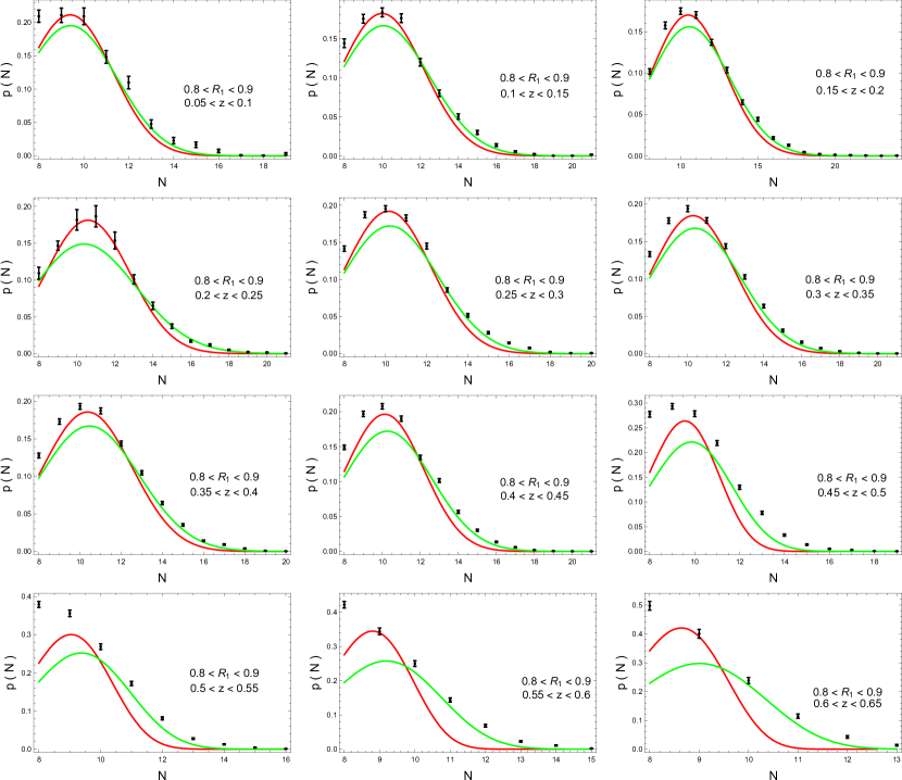
The data points and the errors on the distribution function which we finally obtain are shown respectively as black dots and bars in Figs. (5) - (6) - (7). The best fitting distributions obtained from the minimization of are shown in red; those ones derived from are in green.
The minimization of the defined is performed by using a Monte Carlo Markov Chain (MCMC) approach, running chains with points and using the uninformative and very general priors: ; ; ; .
3.2 Clusters
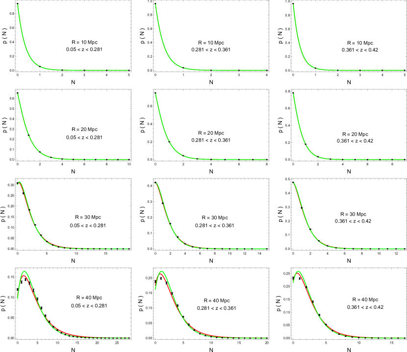
Concerning the count-in-cells where the counted objects within volumes are the clusters of galaxies, we follow a procedure which is very similar to what is described in (Yang and Saslaw, 2011). In order to be as much as clear as possible, we are going to enumerate all the steps in the following list.
The initial set up consists in the coming steps:
-
(1a)
we choose the size of the spherical cells/volumes we are going to analyze. We have selected four different physical lengths, , , , and Mpc;
-
(2a)
we divide the clusters in three groups by redshift, , and . These values have been chosen in order to span approximately the same comoving volume in each group: assuming a baseline Planck cosmology (Aghanim et al., 2020), with km s-1 Mpc-1 and , the volume is Mpc3. The number of clusters from the SDSS catalog falling into each group are, respectively, , and (the total sums up to , because we are taking only clusters with , for which the catalogue is complete);
-
(3a)
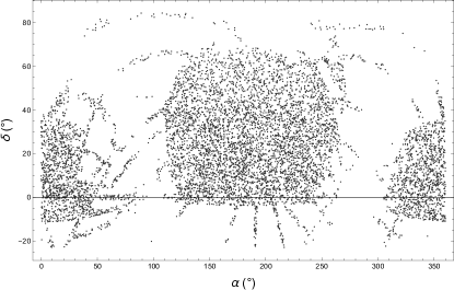
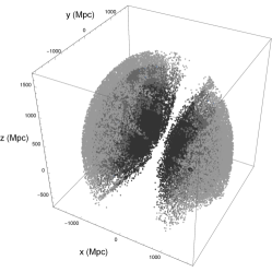
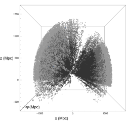
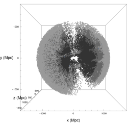
all clusters in the catalog are provided with redshift and celestial coordinates, the right ascension and declination . These quantities are converted into physical Cartesian coordinates using the standard formulae,
(41) where is the comoving distance calculated assuming the same fiducial cosmology as in the previous step. In Fig. 4 we show both the angular projection of the SDSS survey area (top panel), and the “physical length” distribution of the catalogue, with the three bins shown in different colors (bottom panel);
-
(4a)
we define a Cartesian grid covering the SDSS survey area. Each point in this grid will be the center of a cell which will be used for the count-in-cell procedure. In order to guarantee a full coverage of the area, considering that the volumes are spheres, the distance between each point (i.e. each center of each cell) is ;
-
(4a)
the SDSS survey does not cover the sky in a uniform way; thus, we are not going to include in our analysis all the points from the previously defined Cartesian grid. Actually, converting the Cartesian coordinates of each point back to celestial coordinates, we only select those ones which fall in the range defined by the initial cluster catalog. This step will acquire more significance as further steps in our procedure will be highlighted in the next points.
Having defined this initial set up, we have performed the following operations on/with it:
-
(1b)
we randomize the grid defined in the previous point , by shifting its origin by a random number in the interval . Actually, we apply this shift independently to each Cartesian axis of the grid;
-
(2b)
after each shift, we only retain cells which satisfy the condition described in the previous point . This assures us that any cell which should fall out of the SDSS survey will not be considered in the following analysis;
-
(3b)
additionally, we apply a jackknife cut of of cells selected randomly;
-
(4b)
the previous steps, , are realized times, each time having a different shift in the origin of the grid system (point ), a possibly different number of cells falling out of the SDSS survey are (point ), and a different set of cells cut from point .
After all these steps are performed, we eventually have at our disposal the grid of centers of cells/volumes, for each cell size provided at point , and divided in the three subgroups following the redshift criterion described at point , which will serve to perform the count-in-cell with the cluster catalog data. Basically, for each point in the grid, we will retain only the clusters whose distance from a given grid point (i.e. cell center) will be lower than the size taken into account. Because of point above, we basically have different grid sets to compare with the original catalogue, namely, we will have spanning the ranges where, as before, and are the minimum and maximum numbers of objects (clusters) within each cell/volume.
3.3 Results
The complete outcomes of our statistical analysis are presented in Table 1 for galaxies and Table 2 for clusters of galaxies. As a first comment, valid for both cases, let us notice that the softening parameter is not present in the tables because it is basically unconstrained, exhibiting a uniform distribution all over the given prior range . Thus, we can infer that its role in the fit is marginal.
3.3.1 Galaxies
For what concerns galaxies, from Table 1 we can see how the parameter is very well constrained, and there is no difference between using or . This statement is valid whatever radius and redshift bin is considered. Actually, we must remember that the catalog is complete only up to , after which we do have a bias toward smaller clusters, namely, clusters with a lower . And this is effectively seen in the tables, where rises slightly with redshift, becomes practically constant, and then starts to decrease for .
The same consideration is basically true also for the clustering parameter , even if in this case we can see how there is a trend with varying , while no peculiar change with redshift can be detected. In general, this parameter lies in the range for all cases; however, while for the smaller we can see how it is very well constrained, for growing , we are able to put only upper limits on it, which means that also small values of are compatible with data. As described in (Yang and Saslaw, 2012), we know that smaller values of correspond to clusters which have not yet fully virialized. It is worth noticing that such trend is on the opposite side with respect to (Sivakoff and Saslaw, 2005; Rahmani et al., 2009; Yang and Saslaw, 2012) where smaller cells volumes correspond to smaller values of ; although we must also stress that in (Sivakoff and Saslaw, 2005; Rahmani et al., 2009; Yang and Saslaw, 2012), the considered physical volumes are much larger than those we have defined here as well as the redshift bins, and the number of objects in each bin is much lower. In our case the bins are much finer, both in radius and in redshift.
For what concerns the only fully characterizing parameter of the nonlocal gravitational potential, i.e. , we can see how it is remarkably very well constrained in a specific and well defined range. Statistically speaking, we can see how it approximately lies in the range , which, in physical units, corresponds roughly to Mpc. We can detect a slight decrease for varying redshift, with smaller values at larger ; while it seems to be more pronounced a trend with varying , with larger for larger clusters. It is quite striking to have such values for this parameter, which are actually totally consistent with the size of gravitational structures/volumes under scrutiny. At the same time, they are also very different from a stable GR limit, which would be achieved when . Actually, from Eq. 7, one can see how it would be possible to recover an unstable GR-like limit even for .
Finally, from Figs. 5 - 6 - 7, we can also visually check the quality of the fits: the larger is the cell volume, the better is the fit.
We must stress here an important point: these results just show that a logarithmic correction to the Newtonian gravity might be consistent with the clustering of galaxies. But we cannot state at all that this correction is consistent with the full clustering process at these same scales, because, from the catalogue we have used, we have no information on voids, which should be taken into account. This is a further check which should be performed in the future.
3.3.2 Clusters
What we can check is how the full clustering process on larger scales behaves. As we have stated in the previous sections, if we move to consider the clustering of clusters of galaxies, the catalogue in hand does allow us to properly take into account voids. Although, in this case, results are a bit more fuzzy.
First of all, we focus on . We can see here a trend both in redshift and in volume size : decreases with redshift and increases with . The latter correspondence is of course expected, as large cells can contain more clusters; the former one is also somehow expected, because we might predict an intrinsic lack of clusters at higher redshifts, as they are caught in an epoch of formation, while a larger number of them is observable at smaller redshifts. Notice that our bins all have the same comoving volumes, so that any geometry-related issue should not be effective in this case.
The behavior of the clustering parameter is now fully consistent with literature (Sivakoff and Saslaw, 2005; Rahmani et al., 2009; Yang and Saslaw, 2012), with smaller values for smaller volumes, as well as for higher redshifts.
The nonlocal characteristic length , instead, in this case is quite unconstrained. We are unable to put strong boundaries on it and in Table 2 we can only assess upper limits on it. Although we must warn that such results are statistically weak, with the posteriors being quite irregular in most of the cases. This result can only be interpreted as a substantial negligible role of the parameter in the fitting procedure. Thus, we should conclude that on such large scales there is no evidence for a detectable logarithmic correction to the standard Newtonian potential.
| Mpc | Mpc | Mpc | ||||||||||
|---|---|---|---|---|---|---|---|---|---|---|---|---|
| Mpc | Mpc | Mpc | Mpc | ||||||||||
|---|---|---|---|---|---|---|---|---|---|---|---|---|---|
4 Discussion and Conclusions
Nonlocality effects can occur at large distances as the consequence of modified gravitational potential. Specifically, nonlocal gravity, besides the effects at cosmological scale as a possible engine for accelerated expansion (Deser and Woodard, 2007; Bahamonde et al., 2017b), is relevant also for large scale formation. In particular, it is capable of triggering the clustering of galaxies and clusters of galaxies.
In view of this statement, we have analyzed the effects of nonlocal gravitational potential on the structure formation comparing the model with observational data. This has been done by treating both galaxies and clusters of galaxies (in two distinct analysis) as points in a statistical mechanical system, and then analyzing their clustering using a gravitational partition function. This function has been modified according to the nonlocal gravitational potential and its influence on the properties of the gravitational clustering has been scrutinized. Finally, the model has also been compared with observational data, and we have demonstrated that a logarithmic correction to standard gravity seems to be consistent with the observations, at least with those concerning the galactic scale, i.e. within volumes corresponding to clusters of galaxies. Thus, it is possible to conclude that the nonlocal gravitational effects might be revealed at such scales. On the other hand, we must stress that the clustering of larger volumes of space, in which the points are the clusters of galaxies, does not show any evidence in favor of a such modification to gravity so that any inference should be suspended until further (maybe more precise) probes are checked.
For a more general discussion, it has be noted that other modifications of gravitational potential, explaining dark matter or dark energy effects, have been studied considering modifications of the gravitational partition function. For example, it is well-known that gravity modifies the large distance behavior of gravitational potential (Capozziello, 2002; Capozziello and De Laurentis, 2011; Sotiriou and Faraoni, 2010; Nojiri et al., 2017). Thus, the clustering of galaxies, interacting through effective potentials derived from gravity, has also been studied using a modified gravitational partition function, and it has been observed that also these models are consistent with observations for large samples of galaxies and clusters (Capozziello et al., 2009, 2018), although the corresponding statistical inferenec is a bit weaker that the nonlocal scenario we have considered here. It is worth noticing that the clustering of galaxies in gravity is also consistent with the constraints coming from the Planck data (De Martino et al., 2014).
The MOND gravitational partition function has also been used to study the thermodynamics and the clustering properties of systems of galaxies (Upadhyay et al., 2018; Hameeda et al., 2019).
Furthermore, the gravitational phase transition can also be analyzed using the gravitational partition function for systems of galaxies (Khan and Malik, 2012). In fact, a first order phase transition occurs due to the clustering of galaxies from a homogeneous phase. In this framework, it is possible to take into account the Yang-Lee theory for systems of galaxies, and use the complex fugacity to analyze the phase transition (Khan and Malik, 2013). A forthcoming step will be to extend the Yang-Lee theory for nonlocal gravitational potential, and analyze the phase transition for the related gravitational partition function.
In particular, it has to be noted that the clustering of galaxies has also been investigated using the cosmic energy equation (Wahid et al., 2011). As the cosmic energy equation is derived by approximating galaxies as points in a statistical mechanical system, a softening parameter can modify the cosmic energy equation (Ahmad et al., 2009). It has been demonstrated that a large scale modification of the gravitational potential also modifies the cosmic energy equation (Hameeda et al., 2018).
Acknowledgements
SC acknowledgs the support of the Istituto Nazionale di Fisica Nucleare (INFN), sezione di Napoli, iniziative specifiche QGSKY and MOONLIGHT-2.
References
- Frenk et al. (1999) C. S. Frenk et al., Astrophys. J. 525, 554 (1999), arXiv:astro-ph/9906160 .
- Barnes et al. (2017) D. J. Barnes, S. T. Kay, Y. M. Bahé, C. Dalla Vecchia, I. G. McCarthy, J. Schaye, R. G. Bower, A. Jenkins, P. A. Thomas, M. Schaller, R. A. Crain, T. Theuns, and S. D. M. White, Mon. Not. Roy. Astron. Soc. 471, 1088 (2017), arXiv:1703.10907 [astro-ph.GA] .
- Ponman et al. (2003) T. J. Ponman, A. J. R. Sanderson, and A. Finoguenov, Mon. Not. Roy. Astron. Soc. 343, 331 (2003), arXiv:astro-ph/0304048 .
- Voit (2005) G. M. Voit, Rev. Mod. Phys. 77, 207 (2005), arXiv:astro-ph/0410173 .
- Saslaw and Yang (2009) W. C. Saslaw and A. Yang, arXiv e-prints , arXiv:0902.0747 (2009), arXiv:0902.0747 [astro-ph.CO] .
- Saslaw and Fang (1996) W. C. Saslaw and F. Fang, Astrophys. J. 460, 16 (1996).
- Saslaw and Sheth (1993) W. C. Saslaw and R. K. Sheth, Astrophys. J. 409, 504 (1993).
- Rahmani et al. (2009) H. Rahmani, W. C. Saslaw, and S. Tavasoli, Astrophys. J. 695, 1121 (2009), arXiv:0902.1103 [astro-ph.CO] .
- Itoh et al. (1993) M. Itoh, S. Inagaki, and W. C. Saslaw, Astrophys. J. 403, 476 (1993).
- Saslaw et al. (1990) W. C. Saslaw, S. M. Chitre, M. Itoh, and S. Inagaki, Astrophys. J. 365, 419 (1990).
- Saslaw (1986) W. C. Saslaw, Astrophys. J. 304, 11 (1986).
- Saslaw and Ahmad (2010) W. C. Saslaw and F. Ahmad, Astrophys. J. 720, 1246 (2010).
- Upadhyay et al. (2018) S. Upadhyay, B. Pourhassan, and S. Capozziello, Int. J. Mod. Phys. D 28, 1950027 (2018), arXiv:1809.03579 [gr-qc] .
- Khan and Malik (2012) M. S. Khan and M. A. Malik, Mon. Not. Roy. Astron. Soc. 421, 2629 (2012).
- Ahmad and Hameeda (2010) F. Ahmad and Hameeda, Astrophysics and Space Science 330, 227 (2010).
- Hameeda et al. (2021) M. Hameeda, B. Pourhassan, M. C. Rocca, and A. B. Brzo, Eur. Phys. J. C 81, 146 (2021).
- Saslaw and Hamilton (1984) W. C. Saslaw and A. J. S. Hamilton, Astrophys. J. 276, 13 (1984).
- Ahmad et al. (2002) F. Ahmad, W. C. Saslaw, and N. I. Bhat, Astrophys. J. 571, 576 (2002).
- Sivakoff and Saslaw (2005) G. R. Sivakoff and W. C. Saslaw, Astrophys. J. 626, 795 (2005), arXiv:astro-ph/0503509 [astro-ph] .
- Rahmani et al. (2009) H. Rahmani, W. C. Saslaw, and S. Tavasoli, Astrophys. J. 695, 1121 (2009), arXiv:0902.1103 [astro-ph.CO] .
- Ahmad et al. (2006) F. Ahmad, W. C. Saslaw, and M. A. Malik, Astrophys. J. 645, 940 (2006).
- Riess et al. (1998) A. G. Riess et al. (Supernova Search Team), Astron. J. 116, 1009 (1998), arXiv:astro-ph/9805201 .
- Perlmutter et al. (1999) S. Perlmutter et al. (Supernova Cosmology Project), Astrophys. J. 517, 565 (1999), arXiv:astro-ph/9812133 .
- Aghanim et al. (2020) N. Aghanim et al. (Planck), Astron. Astrophys. 641, A6 (2020), arXiv:1807.06209 [astro-ph.CO] .
- Gurzadyan et al. (2020) V. G. Gurzadyan, A. A. Kocharyan, and A. Stepanian, Eur. Phys. J. C 80, 24 (2020), arXiv:2001.02634 [astro-ph.CO] .
- Gurzadyan and Stepanian (2018) V. G. Gurzadyan and A. Stepanian, Eur. Phys. J. C 78, 869 (2018), arXiv:1810.09846 [physics.gen-ph] .
- Gurzadyan and Stepanian (2019a) V. G. Gurzadyan and A. Stepanian, Eur. Phys. J. C 79, 169 (2019a), arXiv:1902.07171 [physics.gen-ph] .
- Gurzadyan and Penrose (2013) V. G. Gurzadyan and R. Penrose, Eur. Phys. J. Plus 128, 22 (2013), arXiv:1302.5162 [astro-ph.CO] .
- Gurzadyan and Stepanian (2019b) V. G. Gurzadyan and A. Stepanian, Eur. Phys. J. C 79, 568 (2019b), arXiv:1905.03442 [astro-ph.CO] .
- Le Delliou et al. (2019) M. Le Delliou, R. J. F. Marcondes, and G. a. B. L. Neto, Mon. Not. Roy. Astron. Soc. 490, 1944 (2019), arXiv:1811.10712 [astro-ph.CO] .
- Boonserm et al. (2020) P. Boonserm, T. Ngampitipan, A. Simpson, and M. Visser, Phys. Rev. D 101, 024050 (2020), arXiv:1909.06755 [gr-qc] .
- Peirani and Pacheco (2008) S. Peirani and J. A. D. F. Pacheco, Astron. Astrophys. 488, 845 (2008), arXiv:0806.4245 [astro-ph] .
- Iliev and Shapiro (2001) I. T. Iliev and P. R. Shapiro, Mon. Not. Roy. Astron. Soc. 325, 468 (2001), arXiv:astro-ph/0101067 .
- Stark et al. (2017) A. Stark, C. J. Miller, and D. Huterer, Phys. Rev. D 96, 023543 (2017), arXiv:1611.06886 [astro-ph.CO] .
- Aguena and Lima (2018) M. Aguena and M. Lima, Phys. Rev. D 98, 123529 (2018), arXiv:1611.05468 [astro-ph.CO] .
- Wen et al. (2020) D. Wen, A. J. Kemball, and W. C. Saslaw, Astrophys. J. 890, 160 (2020), arXiv:2001.06119 [astro-ph.CO] .
- Hameeda et al. (2016) M. Hameeda, S. Upadhyay, M. Faizal, and A. F. Ali, Mon. Not. Roy. Astron. Soc. 463, 3699 (2016), arXiv:1610.07990 [gr-qc] .
- Pourhassan et al. (2017) B. Pourhassan, S. Upadhyay, M. Hameeda, and M. Faizal, Mon. Not. Roy. Astron. Soc. 468, 3166 (2017), arXiv:1704.06085 [gr-qc] .
- Deser and Woodard (2007) S. Deser and R. P. Woodard, Phys. Rev. Lett. 99, 111301 (2007), arXiv:0706.2151 [astro-ph] .
- Ding and Deng (2019) J.-C. Ding and J.-B. Deng, JCAP 2019, 054 (2019), arXiv:1908.11223 [astro-ph.CO] .
- Bahamonde et al. (2017a) S. Bahamonde, S. Capozziello, and K. F. Dialektopoulos, Eur. Phys. J. C 77, 722 (2017a), arXiv:1708.06310 [gr-qc] .
- Bahamonde et al. (2017b) S. Bahamonde, S. Capozziello, M. Faizal, and R. C. Nunes, Eur. Phys. J. C 77, 628 (2017b), arXiv:1709.02692 [gr-qc] .
- Bajardi et al. (2020) F. Bajardi, S. Capozziello, and D. Vernieri, Eur. Phys. J. Plus 135, 942 (2020), arXiv:2011.01317 [gr-qc] .
- Modesto and Rachwał (2017) L. Modesto and L. Rachwał, Int. J. Mod. Phys. D 26, 1730020 (2017).
- Capozziello et al. (2020) S. Capozziello, M. Capriolo, and S. Nojiri, Phys. Lett. B 810, 135821 (2020), arXiv:2009.12777 [gr-qc] .
- Belgacem et al. (2019) E. Belgacem, Y. Dirian, A. Finke, S. Foffa, and M. Maggiore, JCAP 11, 022 (2019), arXiv:1907.02047 [astro-ph.CO] .
- Koshelev (2007) A. S. Koshelev, JHEP 04, 029 (2007), arXiv:hep-th/0701103 .
- Koshelev and Vernov (2012) A. S. Koshelev and S. Y. Vernov, Eur. Phys. J. C 72, 2198 (2012), arXiv:0903.5176 [hep-th] .
- Gielen et al. (2013) S. Gielen, D. Oriti, and L. Sindoni, Phys. Rev. Lett. 111, 031301 (2013), arXiv:1303.3576 [gr-qc] .
- Gielen (2019) S. Gielen, JCAP 02, 013 (2019), arXiv:1811.10639 [gr-qc] .
- Yunes and Siemens (2013) N. Yunes and X. Siemens, Living Rev. Rel. 16, 9 (2013), arXiv:1304.3473 [gr-qc] .
- Chicone and Mashhoon (2016a) C. Chicone and B. Mashhoon, Class. Quant. Grav. 33, 075005 (2016a), arXiv:1508.01508 [gr-qc] .
- Tian and Zhu (2019) S. X. Tian and Z.-H. Zhu, Phys. Rev. D 100, 124059 (2019).
- Dialektopoulos et al. (2019) K. F. Dialektopoulos, D. Borka, S. Capozziello, V. Borka Jovanović, and P. Jovanović, Phys. Rev. D 99, 044053 (2019), arXiv:1812.09289 [astro-ph.GA] .
- Lazar (2020) M. Lazar, Phys. Rev. D 102, 096002 (2020), arXiv:2009.09846 [gr-qc] .
- Amendola et al. (2019) L. Amendola, Y. Dirian, H. Nersisyan, and S. Park, JCAP 03, 045 (2019), arXiv:1901.07832 [astro-ph.CO] .
- Hehl and Mashhoon (2009a) F. W. Hehl and B. Mashhoon, Phys. Rev. D 79, 064028 (2009a), arXiv:0902.0560 [gr-qc] .
- Hehl and Mashhoon (2009b) F. W. Hehl and B. Mashhoon, Phys. Lett. B 673, 279 (2009b), arXiv:0812.1059 [gr-qc] .
- Blome et al. (2010) H.-J. Blome, C. Chicone, F. W. Hehl, and B. Mashhoon, Phys. Rev. D 81, 065020 (2010), arXiv:1002.1425 [gr-qc] .
- Chicone and Mashhoon (2016b) C. Chicone and B. Mashhoon, J. Math. Phys. 57, 072501 (2016b), arXiv:1510.07316 [gr-qc] .
- Shapiro et al. (2005) I. L. Shapiro, J. Sola, and H. Stefancic, JCAP 01, 012 (2005), arXiv:hep-ph/0410095 .
- Famaey and McGaugh (2012) B. Famaey and S. McGaugh, Living Rev. Rel. 15, 10 (2012), arXiv:1112.3960 [astro-ph.CO] .
- Park and Tamaryan (2003) D. K. Park and S. Tamaryan, Phys. Lett. B 554, 92 (2003), arXiv:hep-th/0212023 .
- Soleng (1995) H. H. Soleng, Gen. Rel. Grav. 27, 367 (1995), arXiv:gr-qc/9412053 .
- Fabris and Campos (2009) J. C. Fabris and J. P. Campos, Gen. Rel. Grav. 41, 93 (2009), arXiv:0710.3683 [astro-ph] .
- Calcagni and Modesto (2014) G. Calcagni and L. Modesto, J. Phys. A 47, 355402 (2014), arXiv:1310.4957 [hep-th] .
- Biswas et al. (2012) T. Biswas, J. Kapusta, and A. Reddy, JHEP 12, 008 (2012), arXiv:1201.1580 [hep-th] .
- Soussa and Woodard (2003) M. E. Soussa and R. P. Woodard, Class. Quant. Grav. 20, 2737 (2003), arXiv:astro-ph/0302030 .
- Deffayet et al. (2011) C. Deffayet, G. Esposito-Farese, and R. P. Woodard, Phys. Rev. D 84, 124054 (2011), arXiv:1106.4984 [gr-qc] .
- Deffayet et al. (2014) C. Deffayet, G. Esposito-Farese, and R. P. Woodard, Phys. Rev. D 90, 064038 (2014), [Addendum: Phys.Rev.D 90, 089901 (2014)], arXiv:1405.0393 [astro-ph.CO] .
- Tan and Woodard (2018) L. Tan and R. P. Woodard, JCAP 05, 037 (2018), arXiv:1804.01669 [gr-qc] .
- Kim et al. (2016) M. Kim, M. H. Rahat, M. Sayeb, L. Tan, R. P. Woodard, and B. Xu, Phys. Rev. D 94, 104009 (2016), arXiv:1608.07858 [gr-qc] .
- Bagchi and Fring (2019) B. Bagchi and A. Fring, Int. J. Mod. Phys. B 33, 1950018 (2019), arXiv:1709.04339 [physics.gen-ph] .
- Wen et al. (2012) Z. L. Wen, J. L. Han, and F. S. Liu, Astrophysical J. Supplement 199, 34 (2012), arXiv:1202.6424 [astro-ph.CO] .
- Wen and Han (2015) Z. L. Wen and J. L. Han, Astrophys. J. 807, 178 (2015), arXiv:1506.04503 [astro-ph.GA] .
- Yang and Saslaw (2011) A. Yang and W. C. Saslaw, Astrophys. J. 729, 123 (2011), arXiv:1009.0013 [astro-ph.CO] .
- Yang and Saslaw (2012) A. Yang and W. C. Saslaw, Astrophys. J. 753, 113 (2012), arXiv:1203.3823 [astro-ph.CO] .
- Capozziello (2002) S. Capozziello, Int. J. Mod. Phys. D 11, 483 (2002), arXiv:gr-qc/0201033 .
- Capozziello and De Laurentis (2011) S. Capozziello and M. De Laurentis, Phys. Rept. 509, 167 (2011), arXiv:1108.6266 [gr-qc] .
- Sotiriou and Faraoni (2010) T. P. Sotiriou and V. Faraoni, Rev. Mod. Phys. 82, 451 (2010), arXiv:0805.1726 [gr-qc] .
- Nojiri et al. (2017) S. Nojiri, S. D. Odintsov, and V. K. Oikonomou, Phys. Rept. 692, 1 (2017), arXiv:1705.11098 [gr-qc] .
- Capozziello et al. (2009) S. Capozziello, E. De Filippis, and V. Salzano, Mon. Not. Roy. Astron. Soc. 394, 947 (2009), arXiv:0809.1882 [astro-ph] .
- Capozziello et al. (2018) S. Capozziello, M. Faizal, M. Hameeda, B. Pourhassan, V. Salzano, and S. Upadhyay, Mon. Not. Roy. Astron. Soc. 474, 2430 (2018), arXiv:1711.06630 [astro-ph.CO] .
- De Martino et al. (2014) I. De Martino, M. De Laurentis, F. Atrio-Barandela, and S. Capozziello, Mon. Not. Roy. Astron. Soc. 442, 921 (2014), arXiv:1310.0693 [astro-ph.CO] .
- Hameeda et al. (2019) M. Hameeda, B. Pourhassan, M. Faizal, C. P. Masroor, R. U. H. Ansari, and P. K. Suresh, Eur. Phys. J. C 79, 769 (2019), arXiv:1911.01739 [gr-qc] .
- Khan and Malik (2013) M. S. Khan and M. A. Malik, Astrophysics and Space Science 348, 211 (2013).
- Wahid et al. (2011) A. Wahid, F. Ahmad, and A. Nazir, Astrophysics and Space Science 333, 241 (2011).
- Ahmad et al. (2009) F. Ahmad, A. Wahid, M. A. Malik, and S. Masood, International Journal of Modern Physics D 18, 119 (2009).
- Hameeda et al. (2018) M. Hameeda, S. Upadhyay, M. Faizal, A. F. Ali, and B. Pourhassan, Phys. Dark Univ. 19, 137 (2018), arXiv:1712.08591 [gr-qc] .