Braided Frobenius Algebras from Certain Hopf Algebras

Abstract.

A braided Frobenius algebra is a Frobenius algebra with braiding that commutes with the operations, that are related to diagrams of compact surfaces with boundary expressed as ribbon graphs. A heap is a ternary operation exemplified by a group with the operation $(x,y,z)\mapsto xy^{-1}z$, that is ternary self-distributive. Hopf algebras can be endowed with the algebra version of the heap operation. Using this, we construct braided Frobenius algebras from a class of certain Hopf algebras that admit integrals and cointegrals. For these Hopf algebras we show that the heap operation induces a braiding, by means of a Yang-Baxter operator on the tensor product, which satisfies the required compatibility conditions. Diagrammatic methods are employed for proving commutativity between the braiding and Frobenius operations.

1. Introduction

Frobenius algebras have been studied in recent decades in relation to 2-dimensional topological quantum field theories (TQFTs) [Kock], and to Khovanov homology [Khov] in knot theory, that is a categorification of the Jones polynomial [Jones]. Braid groups have been extensively used in relation to generalizations of the Jones polynomial, and braided monoidal categories have been developed to further extend knot invariants to ribbon graphs [RT], that consist of disk vertices and ribbon edges. Spatial graphs with a move that corresponds to handle slides have been studied for handlebody-links [Ishii]. Corresponding algebraic structures that have multiplication and braiding at the same time, with compatibility conditions, have also been studied [CIST, Lebed]. Compact surfaces with boundary can be represented by ribbon graphs, and their moves [Matsu] and their invariants [IMM] have been studied. For algebraic objects having both Frobenius and braiding structures, Frobenius objects in braided monoidal categories was proposed in [Comeau], and relations to a certain tangle category were discussed.

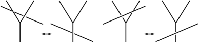
Figure 1. Axioms of a braided Frobenius algebra

Motivated from these developments, in this paper, we present a construction of braided Frobenius algebras from certain Hopf algebras. A braided Frobenius algebra is a Frobenius object in the braided strict monoidal category of modules over unital rings (Definition 5.1). Specifically, a braided Frobenius algebra is a Frobenius algebra $X=(V,\mu,\eta,\Delta,\epsilon)$ (multiplication, unit, comltiplication, counit) over a unital ring ${\mathbb{k}}$, which commute with the braiding, as explicitly formulated below. This commutation is represented by diagrams depicted in Figure 1, where the multiplication and braiding are represented by trivalent vertices and crossings, respectively, and these are part of moves for spatial graph diagrams.

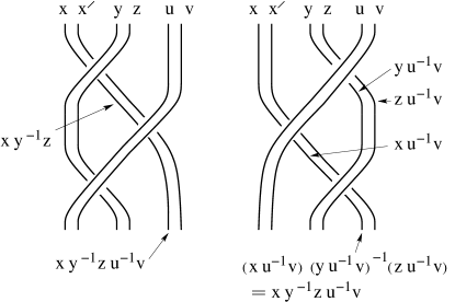
Figure 2. Heap operation and braid relation

The idea of the construction is based on heaps. A heap is an abstraction of a group endowed with the ternary operation $a\times b\times c\mapsto T(a,b,c)=ab^{-1}c$. It is computed that this operation on a group satisfies the ternary self-distributive law (TSD) $T((x,y,z),u,v)=T(T(x,u,v),T(y,u,v)T(z,u,v))$ for all $x,y,z,u,v$. Binary self-distributive operations have been studied in relation to the Yang-Baxter operators through tensor categories (e.g., [CCES]). In [ESZ] a diagrammatic interpretation of TSD was given in terms of framed links, providing set-theoretic Yang-Baxter operators. The assignment of heap elements on arcs and the heap operations to crossings are depicted in Figure 2, together with the TSD property corresponding to a braid relation (the type III Reidemeister move in knot theory). In [ESZheap], the constructions of TSD operations from heaps were generalized to monoidal categories. Those in the category of finite dimensional Hopf algebras over a field are called quantum heaps. We use quantum heaps $X$ to construct a Frobenius algebra structure on $V=X\otimes X$ that commute with braiding induced from the TSD operations. A key method of proofs is extensive use of diagrams.

The paper is organized as follows. In Section 2 we review basic definitions and facts regarding heap structures, Hopf algebras, Frobenius algebras and Yang-Baxter operators. In Section 3 we deal with ternary self-distributive (TSD) structures in coalgebras, and construct a Yang-Baxter operator associated to a TSD structure arising from quantum heaps in Hopf algebras. In Section 4 (co)pairings are constructed that commute with braidings. These (co)pairing are used for (co)units for Frobenius structures. In Section 5 we introduce the notion of braided Frobenius algebra and show that there is a class of these structures arising from quantum heaps where a Frobenius algebra is defined via Hopf algebra (co)integrals. Section 6 discusses relations to compact surfeces with boundary embedded in 3-space, and issues of twists in braided Frobenius algebras.

2. Preliminary

In this section we review materials used in this paper.

2.1. Heaps

We recall the definition and basic properties of heaps. Given a set $X$ with a ternary operation $[-]$, the set of equalities

$$[[x_{1},x_{2},x_{3}],x_{4},x_{5}]=[x_{1},[x_{4},x_{3},x_{2}],x_{5}]=[x_{1},x_{2},[x_{3},x_{4},x_{5}]]$$

is called para-associativity. The equations $[x,x,y]=y$ and $[x,y,y]=x$ are called the degeneracy conditions. A heap is a non-empty set with a ternary operation satisfying the para-associativity and the degeneracy conditions [ESZheap]. A typical example of a heap is a group $G$ where the ternary operation is given by $[x,y,z]=xy^{-1}z$, which we call a group heap.

Let $X$ be a set with a ternary operation $(x,y,z)\mapsto T(x,y,z)$. The condition $T((x,y,z),u,v)=T(T(x,u,v),T(y,u,v)T(z,u,v))$ for all $x,y,z,u,v\in X$, is called ternary self-distributivity, TSD for short. It is known and easily checked that the heap operation $(x,y,z)\mapsto[x,y,z]=T(x,y,z)$ is ternary self-distributive. We focus on the TSD property of heaps.

2.2. Hopf algebras

A Hopf algebra $(X,\mu,\eta,\Delta,\epsilon,S)$ (a module over a unital ring $\mathbb{k}$, multiplication, unit, comultiplication, counit, antipode, respectively), is defined as follows. First, a bialgebra $X$ has a multiplication $\mu:X\otimes X\longrightarrow X$ with unit $\eta$ and a comultiplication $\Delta:X\longrightarrow X\otimes X$ with counit $\epsilon$ such that the compatibility condition $\Delta\circ\mu=(\mu\otimes\mu)\tau\circ(\Delta\otimes\Delta)$ holds. Then a Hopf algebra is a bialgebra endowed with a map $S:X\longrightarrow X$, called antipode, satisfying the equations $\mu\circ(\mathbb{1}\otimes S)\circ\Delta=\eta\circ\epsilon=\mu\circ(S\otimes\mathbb{1})\circ\Delta$, called the antipode condition.

The diagrammatic representation of the algebraic operations appearing in a Hopf algebra is given in Figure 3. Diagrams are read from top to bottom. For example, the top two arcs of the trivalent vertex for $\mu$ (the leftmost diagram) represent $X\otimes X$, the vertex represents $\mu$, and the bottom arc represents $X$. In Figure 4 some of the defining axioms of a Hopf algebra are translated into diagrammatic equalities. Specifically, diagrams represent (A) associativity of $\mu$, (B) unit condition, (C), compatibility between $\mu$ and $\Delta$, (D) the antipode condition. The coassociativity and counit conditions are represented by diagrams that are vertical mirrors of (A) and (B), respectively.

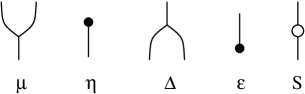
Figure 3. Operations of Hopf algebras

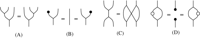
Figure 4. Axioms of Hopf algebras

Any Hopf algebra satisfies the equality $S\mu\tau=\mu(S\otimes S)$, where $\tau$ denotes the transposition $\tau(x\otimes y)=y\otimes x$ for simple tensors. This equality is depicted in Figure 5. A Hopf algebra is called involutory if $S^{2}={\mathbb{1}}$, the identity. It is known, [Kas] Theorem III.3.4, that if a Hopf algebra is commutative or cocommutative it follows that it is also involutory. In what follows, we will not mention that our Hopf algebras are involutory when they are (co)commutative, and freely apply the fact that $S^{2}={\mathbb{1}}$ without further mention.

For the comultiplication, we use Sweedler’s notation $\Delta(x)=x^{(1)}\otimes x^{(2)}$ supressing the summation. Further, we use $(\Delta\otimes{\mathbb{1}})\Delta(x)=(x^{(11)}\otimes x^{(12)})\otimes x^{(2)}$ and $({\mathbb{1}}\otimes\Delta)\Delta(x)=x^{(1)}\otimes(x^{(21)}\otimes x^{(22)})$, both of which are also written as $x^{(1)}\otimes x^{(2)}\otimes x^{(3)}$ from the coassociativity.

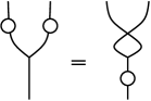
Figure 5. Twisting $\mu$ with antipodes

A left integral of $X$ is an element $\lambda\in X$ such that $x\lambda=\epsilon(x)\lambda$ for all $x\in X$. A right integral, a (two-sided) integral, cointegrals are defined similarly. Diagrams for integral conditions are depicted in Figure 6. The diagram (A) represents an integral, (B) represents the defining equation of a left integral, and similar for cointegrals in (C) and (D). The existence of integrals is a fundamental tool to endow a Hopf algebra with a Frobenius structure (defined below). It is known that the set of integrals of a free finite dimensional Hopf algebra over a PID admits a one dimensional space of integrals, see [LS]. More generally, a finitely generated projective Hopf algebra over a ring admits a left integral space of rank one [Par]. Observe that when a Hopf algebra is (co)commutative, it follows that a left (co)integral is also a right (co)integral.

Figure 6. Left (co)integral of Hopf algebras

2.3. Frobenius algebras

We use the following definition: A Frobenius algebra $(V,\mu,\eta,\Delta,\epsilon)$ is an associative and coassociative coalgebra over a unital ring ${\mathbb{k}}$ with multiplication $\mu$ and comultiplication $\Delta$, respectively, with unit $\eta:{\mathbb{k}}\rightarrow V$ and counit $\epsilon:V\rightarrow{\mathbb{k}}$ with the same conditions as Hopf algebras, such that $\mu$ and $\Delta$ satisfy the Frobenius compatibility condition: $\ (\mu\otimes{\mathbb{1}})({\mathbb{1}}\otimes\Delta)=\Delta\mu=({\mathbb{1}}\otimes\mu)(\Delta\otimes{\mathbb{1}})$. Thid condition is depicted in Figure 7.

Figure 7. Frobenius compatibility condition

2.4. The Yang-Baxter operator

Let $X$ be a module over a ring and let $R:X\otimes X\longrightarrow X\otimes X$ be an operator (i.e. a linear map). The Yang-Baxter equation, YBE for short, for $R$ is the functional equation

$$(R\otimes\mathbb{1})\circ(\mathbb{1}\otimes R)\circ(R\otimes\mathbb{1})=(\mathbb{1}\otimes R)\circ(R\otimes\mathbb{1})\circ(\mathbb{1}\otimes R)$$

where LHS and RHS are both endomorpshism of $X\otimes X\otimes X$. The YBE is well known to be represented by the type III Reidemeister move in knot theory, and has been widely studied in low-dimensional topology because it produces invariants of knots. If the operator $R$ satisfies the YBE, then it is said to be a pre Yang-Baxter operator. If, in addition, $R$ is invertible then we say that $R$ is a Yang-Baxter operator, YB operator for short.

3. Ternary self-distributive operations in coalgebras and braidings

In this section we provide a method of producing braidings from ternary self-distributive (TSD) operations.

Definition 3.1.

[ESZ] A morphism $T:V^{\otimes 3}\rightarrow V$ for a coalgebra $V$ over a unital ring ${\mathbb{k}}$ is called ternary self-distributive (TSD for short) if it satisfies, when expressed in simple tensors,

$$T(T(x\otimes y\otimes z)\otimes u\otimes v)$$

$$= T(T(x\otimes u^{(11)}\otimes v^{(11)})\otimes T(x\otimes u^{(12)}\otimes v^{(12)})\otimes T(x\otimes u^{(2)}\otimes v^{(2)})).$$

Lemma 3.2.

[ESZ] Let $(X,\mu,\Delta,\iota,\epsilon,S)$ be an involutory Hopf algebra. Let $T(x\otimes y\otimes z)=xS(y)z=\mu(\mu(x\otimes S(y))\otimes z)$ expressed in simple tensors, where the concatenation denotes the multiplication. Then $T$ is TSD.

This construction is represented by the diagrams in Figure 8.

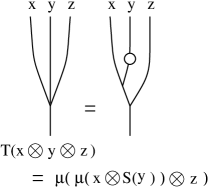
Figure 8. Quantum heap operation as a TSD

Definition 3.3.

A TSD morphism $T:V^{\otimes 3}\rightarrow V$ for a module $V$ over a unital ring ${\mathbb{k}}$ is called invertible if it satisfies

$$T(T(x\otimes y^{(2)}\otimes z^{(2)})\otimes z^{(1)}\otimes y^{(1)})=\epsilon(y)\epsilon(z)\cdot x,$$

for all $x,y,z\in V$.

Lemma 3.4.

Let $(X,\mu,\Delta,\iota,\epsilon,S)$ be an involutory Hopf algebra, and let $T(x\otimes y\otimes z)=xS(y)z$ be as defined in Lemma 3.2. If $(X,\Delta)$ is cocommutative, then $T$ is invertible.

Proof.

One computes

$$T(T(x\otimes y^{(2)}\otimes z^{(2)})\otimes z^{(1)}\otimes y^{(1)})$$

$$=xS(y^{(2)})z^{(2)}S(z^{(1)})y^{(1)}=xS(y^{(2)})S(z^{(1)})z^{(2)}y^{(1)}=\epsilon(z)\cdot xS(y^{(2)})y^{(1)}=\epsilon(y)\epsilon(z)\cdot x$$

as desired. ∎

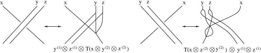
Figure 9. Hopf algebra maps corresponding to crossings

Lemma 3.5.

Let $(X,\Delta)$ be a cocommutative coalgebra over a unital ring ${\mathbb{k}}$. Let $T:X^{\otimes 3}\rightarrow X$ be an invertible TSD coalgebra morphism. Then the map $\beta_{1}:X^{\otimes 3}\rightarrow X^{\otimes 3}$ defined for simple tensors by $\beta_{1}(x\otimes y\otimes z)=y^{(1)}\otimes z^{(1)}\otimes T(x\otimes y^{(2)}\otimes z^{(2)})$ is invertible with the inverse $\beta_{1}^{-1}(y\otimes z\otimes x)=T(x\otimes z^{(2)}\otimes y^{(2)})\otimes y^{(1)}\otimes z^{(1)}$, so that $\beta_{1}\beta_{1}^{-1}={\mathbb{1}}$ and $\beta_{1}^{-1}\beta_{1}={\mathbb{1}}$.

Proof.

The proof is an application of the invertibility condition of $T$. On simple tensors we have

$$\beta_{1}^{-1}\beta_{1}(x\otimes y\otimes z) = \beta_{1}^{-1}(y^{(1)}\otimes z^{(1)}\otimes T(x\otimes y^{(2)}\otimes z^{(2)}))$$

$$= T(T(x\otimes y^{(2)}\otimes z^{(2)})\otimes z^{(12)}\otimes y^{(12)})\otimes y^{(11)}\otimes z^{(11)}$$

$$= T(T(x\otimes y^{(22)}\otimes z^{(22)})\otimes z^{(21)}\otimes y^{(21)})\otimes y^{(1)}\otimes z^{(1)}$$

$$= \epsilon(y^{(2)})\epsilon(z^{(2)})x\otimes y^{(1)}\otimes z^{(1)}$$

$$= x\otimes y\otimes z,$$

which shows that $\beta_{1}^{-1}\beta_{1}=\mathbb{1}$. Similar considerations imply that $\beta_{1}\beta_{1}^{-1}=\mathbb{1}$ as well. ∎

Diagrammatic representations of morphisms $\beta_{1}$ and $\beta_{1}^{-1}$ in Lemma 3.5 are depicted in the left and right of Figure 9, respectively. The first equality $\beta_{1}^{-1}\beta_{1}=\mathbb{1}$ in the lemma is represented by Figure 10.

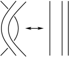
Figure 10. The type II Reidemeister move with a single under-arc and double over-arcs.

Lemma 3.6.

Let $(X,\Delta)$ be a cocommutative coalgebra over a unital ring ${\mathbb{k}}$. Let $T:X^{\otimes 3}\rightarrow X$ be an invertible TSD coalgebra morphism. Let $V=X\otimes X$ be endowed with the tensor coalgebra structure induced by $(X,\Delta)$. Then the map $\beta:V^{\otimes 2}\rightarrow V^{\otimes 2}$ defined for simple tensors by

$$\beta((x\otimes x^{\prime})\otimes(y\otimes z)):=(y^{(1)}\otimes z^{(1)})\otimes T(x\otimes y^{(21)}\otimes z^{(21)})\otimes T(x^{\prime}\otimes y^{(22)}\otimes z^{(22)})$$

satisfies the YBE. Furthermore, there is an inverse

$$\beta^{-1}((y\otimes z)\otimes(x\otimes x^{\prime}))=(T(x\otimes z^{(21)}\otimes y^{(21)})\otimes T(x^{\prime}\otimes z^{(22)}\otimes y^{(22)}))\otimes y^{(1)}\otimes z^{(1)}.$$

Proof.

We show that the YBE holds on simple tensors. Let $x,y,z,w,u,v\in X$, then the LHS of the YBE is computed as

$$(\beta\otimes\mathbb{1})(\mathbb{1}\otimes\beta)(\beta\otimes\mathbb{1})(x\otimes y\otimes z\otimes w\otimes u\otimes v)$$

$$= u^{(1)}\otimes v^{(1)}\otimes T(z^{(1)}\otimes u^{(2)}\otimes v^{(2)})\otimes T(w^{(1)}\otimes u^{(3)}\otimes v^{(3)})$$

$$\hskip 14.22636pt\otimes T(T(x\otimes z^{(2)}\otimes w^{(2)})\otimes u^{(4)}\otimes v^{(4)})$$

$$\hskip 14.22636pt\otimes T(T(y\otimes z^{(3)}\otimes w^{(3)})\otimes u^{(5)}\otimes v^{(5)}).$$

The RHS computed on $x\otimes y\otimes z\otimes w\otimes u\otimes v$ gives

$$(\mathbb{1}\otimes\beta)\circ(\beta\otimes\mathbb{1})\circ(\mathbb{1}\otimes\beta)(x\otimes y\otimes z\otimes w\otimes u\otimes v)$$

$$= u^{(1)}\otimes v^{(1)}\otimes T(z^{(1)}\otimes u^{(4)}\otimes v^{(4)})\otimes T(w^{(1)}\otimes u^{(7)}\otimes v^{(7)})$$

$$\otimes T(T(x\otimes u^{(2)}\otimes v^{(2)})\otimes T(z^{(2)}\otimes u^{(5)}\otimes v^{(5)})\otimes T(w^{(2)}\otimes u^{(8)}\otimes v^{(8)}))$$

$$\otimes T(T(y\otimes u^{(3)}\otimes v^{(3)})\otimes T(z^{(3)}\otimes u^{(6)}\otimes v^{(6)})\otimes T(w^{(3)}\otimes u^{(9)}\otimes v^{(9)})).$$

Rearranging terms by means of the cocommutativity of $\Delta$, using the fact that $T$ is a coalgebra morphism and applying the TSD property of $T$, we see that the two terms coincide, showing that $\beta$ satisfies the YBE.

To show that $\beta$ is invertible observe that, since $\Delta$ is cocommutative, one has $\beta=(\beta_{1}\otimes\mathbb{1})\circ(\mathbb{1}\otimes\beta_{1})$. Similar considerations allow us to write $\beta^{-1}$ as composition of terms where $\beta_{1}^{-1}$ appears. An iteration of Lemma 3.5 then shows that $\beta^{-1}$ is the inverse of $\beta$. ∎

Figure 9 shows the diagrammatic interpretation of the braiding and its inverse in Lemma 3.6 on a single edge of a ribbon. The full braiding, as well as its inverse, is obtained by repeating the procedure on both edges that delimit a ribbon.

Lemma 3.7.

Let $(X,\mu,\eta,\Delta,\epsilon,S)$ be an involutory Hopf algebra. Then the map $\beta:X^{\otimes 2}\rightarrow X^{\otimes 2}$ defined on simple tensors as

$$x\otimes y\otimes z\otimes w\mapsto z^{(1)}\otimes w^{(1)}\otimes xS(z^{(2)})w^{(2)}\otimes yS(z^{(3)})w^{(3)}$$

is a Yang-Baxter operator.

Proof.

The statement follows directly by applying Lemma 3.6 to the quantum heap construction of Lemma 3.2. The invertibility follows from Lemma 3.4. ∎

4. Braidings and pairings in quantum heaps

In this section we introduce pairings and copairings that commute with braiding constructed in the preceding section. We construct such (co)pairing using integrals of Hopf algebras.

Figure 11. The switchback property

Definition 4.1.

A pairing $\cup:V\otimes V\rightarrow\mathbb{k}$ and a copairing $\cap:{\mathbb{k}}\rightarrow V\otimes V$ in a module $V$ over a unital ring $\mathbb{k}$ are said to have (or satisfy) the switchback property if they satisfy the equalities

$$(\cup\otimes{\mathbb{1}})({\mathbb{1}}\otimes\cap)={\mathbb{1}}=({\mathbb{1}}\otimes\cup)(\cap\otimes{\mathbb{1}}).$$

The conditions imply that $\cup$ is non-singular.

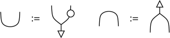
Figure 12. Defining cup and cap by left (co)integrals

Definition 4.2.

Let $(X,\mu,\eta,\Delta,\epsilon,S)$ be a finitely generated projective Hopf algebra over a (unital) ring $\mathbb{k}$. Then $X$ has an integral and a cointegral [Par]. Let us indicate them by $\lambda$ and $\gamma$, respectively. We define a cup on $X$ by $\cup:=\lambda\mu(\mathbb{1}\otimes S)$ and $\cap:=\Delta\gamma$, as depicted in Figure 12.

For a Hopf algebra $(X,\mu,\eta,\Delta,\epsilon,S)$, the following module $P(H^{*})$ was considered in [Par]. Let $\chi:X^{*}\rightarrow X^{*}\otimes X$ be a right $X$-comodule structure on $X^{*}$ defined by the left $H^{*}$-module structure. Then $P(H^{*})$ was defined by $P(H^{*})=\{x^{*}\in X^{*}\mid\chi(x^{*})=x^{*}\otimes 1\}$.

Lemma 4.3.

Let $(X,\mu,\eta,\Delta,\epsilon,S)$ be a finitely generated projective Hopf algebra over a ring $\mathbb{k}$, such that $P(X^{*})\cong{\mathbb{k}}$, and $\cup$, $\cap$ be as in Definition 4.2. Then $\cup$ and $\cap$ satisfy the switchback property.

Proof.

In [Par], it is proved, under the assumptions, that there exists an integral $\lambda$ and cointegral $\gamma$ such that $\cup^{\prime}=\lambda\mu$ and $\cap^{\prime}=(S\otimes{\mathbb{1}})\Delta\gamma$ satisfy the switchback property. It then follows that so do $\cup$ and $\cap$ in Definition 4.2 as well. ∎

Since we use this lemma extensively from here forward, we will assume that every Hopf algebra satisfies the assumption of this lemma. As pointed out in [Par], the condition that $P(H^{*})\cong\mathbb{k}$ is automatically satisfied when ${\rm pic}(\mathbb{k})=0$. This is the case for instance when $\mathbb{k}$ is a PID or a local ring. In particular, one obtains the result of Larson and Sweedler in [LS], where the ground ring is taken to be a PID.

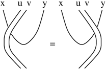
Figure 13. The passcup property

Definition 4.4.

Let $V$ be a coalgebra over a unital ring $\mathbb{k}$, with ternary morphism (of coalgebras) $T:V^{\otimes 3}\rightarrow V$. A pairing $\cup:V\otimes V\rightarrow\mathbb{k}$ is said to have (or satisfy) the passcup property with respect to $T$ if it satisfies

$$({\mathbb{1}}^{\otimes 2}\otimes\cup)(u^{(1)}\otimes v^{(1)}\otimes T(x\otimes u^{(2)}\otimes v^{(2)})\otimes y)=(\cup\otimes{\mathbb{1}}^{\otimes 2})(x\otimes T(y\otimes v^{(2)}\otimes u^{(2)})\otimes u^{(1)}\otimes v^{(1)})$$

for all $x,y,u,v\in V$.

The passcup property is depicted in Figure 13.

Lemma 4.5.

Let $(X,\mu,\eta,\Delta,\epsilon,S)$ be a cocommutative Hopf algebra. Then the pairing $\cup$ defined in Definition 4.2 satisfies the passcup property with respect to the TSD defined in Lemma 3.2.

Proof.

In order to prove the passcup property, we proceed as in Figure 14. The first equality corresponds to rewriting one negative crossing using the definition of inverse of quantum heap operation $T$, the first arrow utilizes naturality of the switching map $X\otimes X\rightarrow X\otimes X$, the second arrow corresponds to the compatibility relation between the antipode $S$ and the comultiplication $\Delta$ of $X$, the third arrow is given by redrawing the diagram using naturality of switching map, the fourth arrow corresponds to the fact that $\lambda$ is both a right and left integral. Involutority is used at Step (3). This completes the proof of the passcup property. ∎

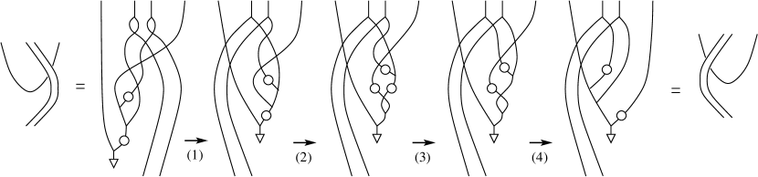
Figure 14. Proof of the passcup property

Lemma 4.6.

Let $(X,\mu,\eta,\Delta,\epsilon,S)$ be a commutative and cocommutative Hopf algebra and set $V=X\otimes X$. Then the cup and cap defined in Definition 12 commute with the braiding defined in Lemma 3.7. Specifically, it holds that $({\mathbb{1}}\otimes\cup)\beta=\cup\otimes{\mathbb{1}}$ and $(\cup\otimes{\mathbb{1}})\beta={\mathbb{1}}\otimes\cup$ as morphisms $V\otimes V\rightarrow V$, $({\mathbb{1}}\otimes\cap)\beta=\cap\otimes{\mathbb{1}}$ and $\beta(\cap\otimes{\mathbb{1}})={\mathbb{1}}\otimes\cap$ as morphisms $V\rightarrow V\otimes V$.

Proof.

Diagrammatic sketch proofs are found in Figures 15 through 18. In Figure 15, $({\mathbb{1}}\otimes\cup)\beta=\cup\otimes{\mathbb{1}}$ is proved by Lemmas 4.5 and 3.5 successively. Other equalities are proved as depicted, using Hopf algebra axioms and the definition of integrals. In Figure 16, other than axioms, commutativity is used in the 4th equality, and cocommutativity is used in the 5th equality. While the diagrams in Figures 16 and 17 treat the single-stranded case, an iteration of the diagrammatic proof implies the case with two edges sliding. Cocommutativity is used in the 3rd and 5th equalities in Figure 17, and 3rd equality in Figure 18. Observe that the equalities $S\eta=\eta$ and $\epsilon S=\epsilon$, which are consequences of $S$ being an anti-homomorphism, have been used. ∎

Figure 15. Proof of $({\mathbb{1}}\otimes\cup)\beta=\cup\otimes{\mathbb{1}}$

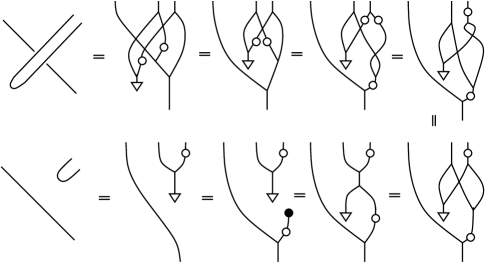
Figure 16. Proof of $(\cup\otimes{\mathbb{1}})\beta={\mathbb{1}}\otimes\cup$

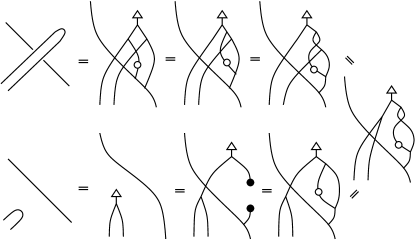
Figure 17. Proof of $({\mathbb{1}}\otimes\cap)\beta=\cap\otimes{\mathbb{1}}$

Figure 18. Proof of $\beta(\cap\otimes{\mathbb{1}})={\mathbb{1}}\otimes\cap$

5. Construction of braided Frobenius algebras

In [Comeau], a braided Frobenius object is defined to be a Frobenius object in a braided monoidal category. A monoidal category has (tensor) products among objects, with some other data and conditions, such as unitors and associators, corresponding to units and associativity of algebras. A monoidal category is strict if its associators and left/right unitors are identity natural transformations. A braided monoidal category has a braiding between (tensor) products of two objects, that are functorial. Hence it is natural to define a braided Frobenius algebra to be a Frobenuis object in the braided strict monoidal category of finitely generated modules over a unital ring. This definition is equivalent to having a braiding $\beta$ that commutes with all defining data of a Frobenius algebra, that corresponds to functoriality of braiding.

Definition 5.1.

(cf. [Comeau]) A braided Frobenius algebra is a Frobenuis object in the braided strict monoidal category of finitely generated projective modules over a unital ring. Specifically, a braided Frobenius algebra is a Frobenius algebra $X=(V,\mu,\eta,\Delta,\epsilon)$ (multiplication, unit, comltiplication, counit) over unital ring ${\mathbb{k}}$, which commute with the braiding, as follows:

$\begin{array}[]{cc}(\mu\otimes\mathbb{1})({\mathbb{1}}\otimes\beta)(\beta\otimes{\mathbb{1}})=\beta\otimes(\mathbb{1}\otimes\mu),&(\mathbb{1}\otimes\mu)(\beta\otimes{\mathbb{1}})({\mathbb{1}}\otimes\beta)=\beta\otimes(\mu\otimes{\mathbb{1}}),\\ (\Delta\otimes{\mathbb{1}})\beta=(\beta\otimes{\mathbb{1}})(\beta\otimes{\mathbb{1}})({\mathbb{1}}\otimes\Delta),&({\mathbb{1}}\otimes\Delta)\beta=(\beta\otimes{\mathbb{1}})(\beta\otimes{\mathbb{1}})(\Delta\otimes{\mathbb{1}}),\\ ({\mathbb{1}}\otimes\eta)\beta=\eta\otimes{\mathbb{1}},&\beta(\eta\otimes{\mathbb{1}})={\mathbb{1}}\otimes\eta,\\ \ ({\mathbb{1}}\otimes\epsilon)\beta=\epsilon\otimes{\mathbb{1}},&(\epsilon\otimes{\mathbb{1}})\beta={\mathbb{1}}\otimes\epsilon.\end{array}$

Figure 19. Commutation of (co)unit and braiding

The commuting conditions for a braided Frobenius algebra for multiplication are depicted in Figure 1. Those for comultiplication are represented by the upside down diagrams. The commuting conditions for the (co)unit are depicted in Figure 19.

We now proceed to construct a family of braided Frobenius algebras from a class of Hopf algebras. We mention that the monoid structure in the next theorem also appears in Sections 4 and 5 of [HV], under the name of pair of pants monoid, for dagger pivotal categories. In our construction, the fact that Frobenius monoids (e.g. algebras) are self-dual allows us to discard the duality in $X^{*}\otimes X$.

Theorem 5.2.

Let $(X,\mu,\eta,\Delta,\epsilon,S)$ be a commutative and cocommutative Hopf algebra. Then $V=X\otimes X$ has a braided Frobenius algebra structure.

Proof.

Since $X$ is an involutory Hopf algebra, applying Lemma 3.7 it follows that $X\otimes X$ has a braiding $\beta$ that is induced by the quantum heap structure of $X$. We define a product $\mu_{\otimes 2}:X^{\otimes 2}\otimes X^{\otimes 2}\rightarrow X^{\otimes 2}$ by means of $\cup$ as

$$\mu_{\otimes 2}:=\mathbb{1}\otimes\cup\otimes\mathbb{1}.$$

The coproduct $\Delta_{\otimes 2}:X^{\otimes 2}\rightarrow X^{\otimes 2}\otimes X^{\otimes 2}$ is obtained from $\cap$ by the definition

$$\Delta_{\otimes 2}:=\mathbb{1}\otimes\cap\otimes\mathbb{1}.$$

Product is associative since

$$\mu_{\otimes 2}\circ(\mu_{\otimes 2}\otimes\mathbb{1}^{\otimes 2}) = (\mathbb{1}\otimes\cup\otimes\mathbb{1})\circ(\mathbb{1}\otimes\cup\otimes\mathbb{1}\otimes\mathbb{1}^{\otimes 2})$$

$$= \mathbb{1}\otimes\cup\otimes\cup\otimes\mathbb{1}$$

$$= (\mathbb{1}\otimes\cup\otimes\mathbb{1})\circ(\mathbb{1}^{\otimes 2}\otimes\mathbb{1}\otimes\cup\otimes\mathbb{1})$$

$$= \mu_{\otimes 2}\circ(\mathbb{1}^{\otimes 2}\otimes\mu_{\otimes 2}).$$

Similarly, we see that $\Delta_{\otimes 2}$ is coassociative. The fact that $\mu_{\otimes 2}$ and $\Delta_{\otimes 2}$ satisfy the Frobenius laws is seen directly, as we have that $\Delta_{\otimes 2}\circ\mu_{\otimes 2}$, $(\mathbb{1}^{\otimes 2}\otimes\mu_{\otimes 2})\circ(\Delta_{\otimes 2}\otimes\mathbb{1}^{\otimes 2})$ and $(\mu_{\otimes 2}\otimes\mathbb{1}^{\otimes 2})\circ(\mathbb{1}^{\otimes 2}\Delta_{\otimes 2})$ evaluated on simple tensors $x\otimes y\otimes z\otimes w$ all equal

$$\cup(y\otimes z)\cdot x\otimes\cap(1)\otimes w,$$

where we have used $\cdot$ to separate an element of the ground ring $\mathbb{k}$ from elements of $X^{\otimes 4}$ to avoid confusion.

Figure 20. The unit axiom

The unit $\eta_{\otimes 2}:{\mathbb{k}}\rightarrow X^{\otimes 2}\otimes X^{\otimes 2}$ is defined by $\cap$. The unit condition follows from the switchback condition, as depicted in Figure 20. The counit $\epsilon_{\otimes 2}$ is defined by $\epsilon_{\otimes 2}=\cup$ and the counit condition follows similarly. Hence $X\otimes X$ is endowed with a Frobenius structure and a braiding induced from the quantum heap operation.

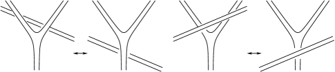
Figure 21. Braided Frobenius conditions for a doubled Hopf algebra

To complete the proof we need to show that braiding and Frobenius morphisms commute in the sense of Definition 5.1. The commutations between (co)units and braiding follow from Lemma 4.6 (see Figures 15 through 18). For doubled strands, the commutations between multiplication and braiding are depicted in Figure 21. These follow from commutations between counits and braiding. The commutations between comultiplication and braiding are represented by the upside down (the vertical mirror) figures of Figure 21, and follow from commutations between units and braiding. ∎

Example 5.3.

Let $X={\mathbb{k}}[G]$ be a group ring of a group heap $G$ with the TSD operation defined by linearlization of the group heap operation $T(x\otimes y\otimes z):=xy^{-1}z$ for $x,y,z\in G$. Endow $X$ with the Hopf algebra structure, where $\mu$ is defined by the linearlized group multiplication, group $\Delta(x)=x\otimes x$ for $x\in G$, unit defined by $\eta(1)=e\in G$ (the identity element), and counit defined by $\epsilon(x)=1$ for $x\in G$. The integral is defined by $\sum_{x\in G}x$ and cointegral by $e\mapsto 1$, $e\neq g\mapsto 0$. All conditions in Theorem 5.2 are checked. The braiding is defined from $T$, and for group elements $\beta((x\otimes y)\otimes(u\otimes v))=(u\otimes v)\otimes(xu^{-1}v\otimes yu^{-1}v)$. Thus the braiding is the linearlization of group heap braiding as depicted in Figure 2. If the group $G$ is abelian, $X$ satisfies the assumption of Theorem 5.2. Moreover, so does the dual Hopf algebra ${\mathbb{k}}[G]^{*}$.

Example 5.4.

Let $\mathbb{k}$ be a PID or a local ring of characteristic $p$. Then the truncated polynomial algebra $H=\mathbb{k}[X]/(X^{p^{k}})$ is a finitely genereated free (hence projective) Hopf algebra for any $k\geq 1$. As previously pointed out, $H$ satisfies $P(X^{*})\cong{\mathbb{k}}$ since $\mathbb{k}$ is either a PID or a local ring. We can therefore apply Lemma 4.3 and Theorem 5.2, since $H$ is commutative and cocommutative. Explicitly, the algebra structure of $H$ is determined by multiplication of polynomials, the comultiplication is obtained extending $\Delta(X)=1\otimes X+X\otimes 1$ to be an algebra homomorphism (note that it is here crucial that $H$ is truncated at a power of the characteristic of the ground ring), the counit is defined by $\epsilon(1)=1$, $\epsilon(X)=0$ and the antipode is given by $S(X)=-X$. This construction can be generalized to truncated polynomial algebras with more than one indeterminate.

We note that considering local rings gives a wider class of objects with respect to that of PID’s in [LS]. For instance, the ring ${\mathbb{Z}}_{p}[Y_{1},Y_{2}]/(Y_{1},Y_{2})^{2}$ is a local ring that is not a PID to which the previous construction can be applied.

6. Twists in braided Frobenius algebras

In this section we introduce twists in braided Frobenius algebras, and discuss relations to tortile category structure and surfaces with boundary embedded in 3-space.

Definition 6.1.

Let $(V,\Delta,\epsilon)$ be a finite dimensional coalgebra over a field ${\mathbb{k}}$ with a TSD operation $T:V^{\otimes 3}\rightarrow V$ (Definition 3.1). Then the operation $\theta:V\otimes V\rightarrow$ defined by

$$\theta(x\otimes y) = T(x^{(1)}\otimes x^{(2)}\otimes y^{(2)})\otimes T(y^{(1)}\otimes x^{(3)}\otimes y^{(3)})$$

is called a twist by $T$.

Remark 6.2.

The twisting introduced in Definition 6.1 is motivated from a “quantum” version of the core quandle [FR] operation $(x,y)\mapsto yx^{-1}y$ defined on groups. In fact we have

$$x\otimes y \mapsto x^{(1)}S(x^{(2)})y^{(2)}\otimes y^{(1)}S(x^{(3)})y^{(3)}$$

$$= \epsilon(x^{(1)})y^{(2)}\otimes y^{(1)}S(x^{(2)})y^{(3)}$$

$$= y^{(2)}\otimes y^{(1)}S(x)y^{(3)},$$

where the second term in the tensor product can be identified with the core quandle operation between $y^{(1)}$ and $x$.

Figure 22. Twisting a ribbon

The operation $\theta$ is written by maps as follows. Fix a basis $\{e_{i}:i=1,\ldots,n\}$ for $V$, and define the pairing $\vee:V\otimes V^{*}\rightarrow{\mathbb{k}}$ for the dual space $V^{*}$ by $\vee(x_{i}\otimes x_{j}^{*})=\delta_{i,j}$ with the Kronecker’s delta, and copairing $\wedge:{\mathbb{k}}\rightarrow V\otimes V^{*}$ by $\wedge(1)=\sum_{i=1}^{n}x_{i}\otimes x^{*}_{i}$. Then $\theta$ is written as

$$\theta=({\mathbb{1}}^{\otimes 2}\otimes\vee)({\mathbb{1}}^{\otimes 3}\otimes\vee\otimes{\mathbb{1}})(\beta\otimes{\mathbb{1}}^{\otimes 2})({\mathbb{1}}^{\otimes 3}\otimes\wedge\otimes{\mathbb{1}})({\mathbb{1}}^{\otimes 2}\otimes\wedge)$$

with the braiding $\beta$ induced from $T$ (Lemma 3.6). Diagrammatically, $\theta$ is represented by Figure 22, and corresponds to a full twist as in the right of the figure. In the figure, the maxima and minima corresponds to $\wedge$ and $\vee$, respectively, and indicated by such notations, to distinguish them from $\cap$ and $\cup$.

Proposition 6.3.

Let $(V,\Delta,\epsilon)$ be a cocommutative coalgebra over a unital ring ${\mathbb{k}}$ with a TSD operation $T:V^{\otimes 3}\rightarrow V$ (Definition 3.1). Let $\theta$ be the twist in Definition 6.1. Then $\theta$ commutes with the braiding $\beta$ induced from $T$. Specifically, we have $\beta(\theta\otimes{\mathbb{1}})=({\mathbb{1}}\otimes\theta)\beta$ and $\beta({\mathbb{1}}\otimes\theta)=(\theta\otimes{\mathbb{1}})\beta$.

Proof.

On simple tensors we have

$$\beta(\theta\otimes{\mathbb{1}})(x\otimes y\otimes z\otimes w) = \beta(T(x^{(1)}\otimes x^{(2)}\otimes y^{(2)})\otimes T(y^{(1)}\otimes x^{(3)}\otimes y^{(3)})\otimes z\otimes w)$$

$$= z^{(1)}\otimes w^{(1)}\otimes T(T(x^{(1)}\otimes x^{(2)}\otimes y^{(2)})\otimes z^{(2)}\otimes w^{(2)})$$

$$\hskip 14.22636pt\otimes T(T(y^{(1)}\otimes x^{(3)}\otimes y^{(3)})\otimes z^{(3)}\otimes w^{(3)}),$$

and also

$$({\mathbb{1}}\otimes\theta)\beta(x\otimes y\otimes z\otimes w) = ({\mathbb{1}}\otimes\theta)(z^{(1)}\otimes w^{(1)}\otimes T(x\otimes z^{(2)}\otimes w^{(2)})\otimes T(y\otimes z^{(3)}\otimes w^{(3)}))$$

$$= z^{(1)}\otimes w^{(1)}\otimes T(T(x^{(1)}\otimes z^{(21)}\otimes w^{(21)})\otimes T(x^{(2)}\otimes z^{(22)}\otimes w^{(22)})$$

$$\hskip 14.22636pt\otimes T(y^{(2)}\otimes z^{(32)}\otimes w^{(32)}))\otimes T(T(y^{(1)}\otimes z^{(31)}\otimes w^{(31)})$$

$$\hskip 14.22636pt\otimes T(x^{(3)}\otimes z^{(23)}\otimes w^{(23)})\otimes T(y^{(3)}\otimes z^{(33)}\otimes w^{(33)})),$$

where the fact that, by definition, $T$ is a coalgebra morphism has been applied. Applying cocommutativity of $\Delta$ we can rearrange the $z$ and $w$ terms in such a way that $\beta(\theta\otimes{\mathbb{1}})(x\otimes y\otimes z\otimes w)$ and $({\mathbb{1}}\otimes\theta)\beta(x\otimes y\otimes z\otimes w)$ differ by an application of the TSD condition of $T$ utilized twice. This shows the equality $\beta(\theta\otimes{\mathbb{1}})=({\mathbb{1}}\otimes\theta)\beta$.

Let us now consider the equation $\beta({\mathbb{1}}\otimes\theta)=(\theta\otimes{\mathbb{1}})\beta$. For the LHS we have

$$\beta({\mathbb{1}}\otimes\theta)(x\otimes y\otimes z\otimes w) = T(z^{(11)}\otimes z^{(21)}\otimes w^{(21)})\otimes T(w^{(11)}\otimes z^{(31)}\otimes w^{(31)})$$

$$\hskip 14.22636pt\otimes T(x\otimes T(z^{(12)}\otimes z^{(22)}\otimes w^{(22)})\otimes T(w^{(12)}\otimes z^{(32)}\otimes w^{(32)})$$

$$\hskip 14.22636pt\otimes T(y\otimes T(z^{(13)}\otimes z^{(23)}\otimes w^{(23)})\otimes T(w^{(13)}\otimes z^{(33)}\otimes w^{(33)}),$$

while for the RHS we have

$$(\theta\otimes{\mathbb{1}})\beta(x\otimes y\otimes z\otimes w) = T(z^{(11)}\otimes z^{(12)}\otimes w^{(12)})\otimes T(w^{(11)}\otimes z^{(13)}\otimes w^{(13)})$$

$$\hskip 14.22636pt\otimes T(x\otimes z^{(2)}\otimes w^{(2)})\otimes T(y\otimes z^{(3)}\otimes w^{(3)}).$$

To complete the proof we see that it is enough to show the equality

(1) $$T(x\otimes T(z^{(1)}\otimes z^{(2)}\otimes w^{(2)})\otimes T(w^{(1)}\otimes z^{(3)}\otimes w^{(3)})) = T(x\otimes z\otimes w).$$

We have

$$T(x\otimes T(z^{(1)}\otimes z^{(2)}\otimes w^{(2)})\otimes T(w^{(1)}\otimes z^{(3)}\otimes w^{(3)}))$$

$$= \epsilon(z^{(2)})\epsilon(w^{(2)})\cdot T(x\otimes T(z^{(1)}\otimes z^{(3)}\otimes w^{(3)})\otimes T(w^{(1)}\otimes z^{(4)}\otimes w^{(4)}))$$

$$= T(T(T(x\otimes w^{(3)}\otimes z^{(3)})\otimes z^{(2)}\otimes w^{(2)})\otimes T(z^{(1)}\otimes z^{(4)}\otimes w^{(4)})\otimes T(w^{(1)}\otimes z^{(5)}\otimes w^{(5)})),$$

where the first equality uses the definition of counit $\epsilon$, and the second equality makes use of the invertibility condition of $T$. Let us now apply the TSD property of $T$ to the terms $T(x\otimes w^{(2)}\otimes z^{(2)})$, $z^{(1)}$, $w^{(1)}$, $z^{(3)}$ and $w^{(3)}$, where we set $T(x\otimes w^{(3)}\otimes z^{(3)})=q$ for convenience. We get

$$T(T(q\otimes z^{(2)}\otimes w^{(2)})\otimes T(z^{(1)}\otimes z^{(4)}\otimes w^{(4)})\otimes T(w^{(1)}\otimes z^{(5)}\otimes w^{(5)}))$$

$$=T(T(q\otimes z^{(2)}\otimes w^{(2)})\otimes z^{(1)}\otimes w^{(1)})=\epsilon(z^{(1)})\epsilon(w^{(1)})\cdot T(x\otimes z^{(2)}\otimes w^{(2)})=T(x\otimes z\otimes w),$$

where invertibility of $T$, as well as cocommutativity of $\Delta$, has been used in the second equality. This shows that Equation (1) holds. ∎

Figure 23. Twisting a doubled ribbon

Remark 6.4.

Here we discuss relations to the tortile category. A braided monoidal category is called tortile [JS] (or ribbon [HV]) if there is a morphism $\theta_{X}$ called a twist for every object $X$ such that $\theta_{X,Y}=\beta_{Y,X}\beta_{X,Y}(\theta_{X}\otimes\theta_{Y})$ for all objects $X,Y$, where $\beta$ denotes the braiding.

Let $(V,\Delta,\epsilon)$ be a finite dimensional coalgebra over a field ${\mathbb{k}}$ with a TSD operation $T:V^{\otimes 3}\rightarrow V$ (Definition 3.1). Then Proposition 6.3 implies that the subcategory generated by $V$ in the category of braided monoidal category of finite dimensional coalgebras with TSDs forms a tortile category. The twist $\theta_{\otimes k}$ on $V^{\otimes k}$ is defined by parallel loops, that are defined by taking $k$-fold parallel ribbons. The case $k=2$ is depicted in Figure 23 left. The equality $\theta_{V,V}=\beta_{V,V}\beta_{V,V}(\theta_{V}\otimes\theta_{V})$ is indicated in the figure. The fact that full twist of parallel strings form a tortile category is pointed out in [JS]. In [JS] the twists are defined by parallel loops, that topologically correspond to full twists of parallel strings, using dual spaces. Thus the construction of this twists are obtained by applying the twists in [JS] to braiding defined by TSD operations on coalgebras.

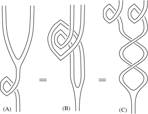
Figure 24. Commutation between a twist and multiplication

Proposition 6.5.

Let $X$ be as in Theorem 5.2, and let $V=X\otimes X$ denote the associated braided Frobenius structure on the doubled vector space. Let $\theta$ be the twist in Definition 6.1. Then the twist $\theta$ commutes with the multiplication and comultiplication. This means, with notations as in Remark 6.4, that $\theta_{V}\,\mu_{\otimes 2}=\mu_{\otimes 2}\,\theta_{V,V}$ and $\Delta_{\otimes 2}\theta_{V}=\theta_{V,V}\Delta_{\otimes 2}$ hold.

The commutation between the twist and multiplication is depicted in the left equality $(A)=(B)$ of Figure 24. The right equality $(B)=(C)$ is a consequence of Figure 23. We note that the resulting equality $(A)=(C)$ corresponds diagrammatically to twisting the trivalent vertex by one full twist.

Proof.

We verify equality $\theta_{V}\,\mu_{\otimes 2}=\mu_{\otimes 2}\,\theta_{V,V}$ on simple tensors $x\otimes y\otimes z\otimes w$. For the LHS we have

$$\theta_{V}\,\mu_{\otimes 2}(x\otimes y\otimes z\otimes w) = \gamma(yS(z))\cdot w^{(2)}\otimes w^{(1)}S(x)w^{(3)}.$$

The RHS is given as

$$\mu_{\otimes 2}\,\theta_{V,V}(x\otimes y\otimes z\otimes w) = \gamma(y^{(1)}S(x^{(3)})y^{(3)}S(z^{(3)})w^{(3)}S(w^{(4)})z^{(4)}S(y^{(4)})x^{(4)}S(z^{(1)}))$$

$$\cdot x^{(1)}S(x^{(2)})y^{(2)}S(z^{(2)})w^{(2)}\otimes w^{(1)}S(x^{(5)})y^{(5)}S(z^{(5)})w^{(5)}$$

$$= \gamma(y^{(1)}S(z^{(1)}))\cdot y^{(2)}S(z^{(2)})w^{(2)}\otimes w^{(1)}S(x)y^{(3)}S(z^{(3)})w^{(3)}$$

$$= \gamma(yS(z))\cdot w^{(2)}\otimes w^{(1)}S(x)w^{(3)},$$

where the first equality is obtained by unraveling the definitions, the second equality is a multiple application of the counit axiom, and the third equality follows by applying the definition of cointegral $\gamma$ twice. Equality $\Delta_{\otimes 2}\theta_{V}=\theta_{V,V}\Delta_{\otimes 2}$ is proven on simple tensors in a similar fashion. ∎

Figure 25. Twisting a ribbon by a loop

Remark 6.6.

For the braided Frobenius algebra $V$ constructed in Theorem 5.2, a twist $\Theta$ can be defined using $\cap$ and $\cup$ instead of $\wedge$ and $\vee$ as depicted in Figure 25 left. Specifically,

$$\Theta=({\mathbb{1}}^{\otimes 2}\otimes\cup)({\mathbb{1}}^{\otimes 3}\otimes\cup\otimes{\mathbb{1}})(\beta\otimes{\mathbb{1}}^{\otimes 2})({\mathbb{1}}^{\otimes 3}\otimes\cap\otimes{\mathbb{1}})({\mathbb{1}}^{\otimes 2}\otimes\cap)$$

with the braiding $\beta$ induced from $T$ (Lemma 3.6). Since all maps that appear in this formula commute with the braiding $\beta$ from earlier lemmas, $\Theta$ commute with $\beta$. By the same argument as Remark 6.4, we obtain a tortile category from $V$. Similarly, $\Theta$ commutes with $\mu$ and $\Delta$. A sketch proof of the commutation between $\mu$ and $\Theta$ is depicted in Figure 26.

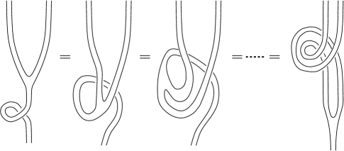
Figure 26. Sketch picture proof of commutation

We close the paper with remarks on invariants of embedded surfaces with boundary. It is of interest to find invariants of compact orientable surfaces with boundary represented by ribbon graph diagrams, as considered in [Matsu], in a way analogous to quantum invariants using braided Frobenius algebras. In this approach, a height function is fixed on the plane, and building blocks of diagrams consist of cups and caps in addition to crossings and trivalent vertices. Although a complete set of moves for ribbon graph diagrams for certain embedded surfaces was given in [Matsu], height functions were not considered. It is desirable to have a list of additional moves. For example, the passcup move and passcap move (the upside down of passcup) are such moves, and they are satisfied by braided Frobenius algebras constructed in this paper. Another move depicted in Figure 27 is also satisfied from Frobenius algebra axioms. Although most moves in [Matsu] for orientable surfaces (without half twists), with appropriate choices of height functions, are satisfied by our resulting braided Frobenius algebras, it is not clear at this time whether the equation corresponding to the move depicted in Figure 28 is satisfied, in general, under our construction. However, it may be satisfied by some specific examples, and may provide invariants for such surfaces.

Figure 27. Conversion of $\mu$ to $\Delta$ through $\cap$

Figure 28. Canceling a pair of loops

For non-orientable surfaces, ribbon graph diagrams [Matsu] contain half-twists, and there is a move of twisting a vertex as indicated in Figure 29, that involve half twists of ribbons merging at a vertex. From the topological correspondence of the twist $\theta$ to a full twists as in Figure 25, such a hypothetical half twist, which we denote by $\sqrt{\theta}$, would be required to satisfy $\sqrt{\theta}\circ\sqrt{\theta}=\theta$ (thus the notation). We have not found such a morphism in braided Frobenius algebras constructed in Theorem 5.2, and raise a question: For the twists ($\theta$ and $\Theta$) defined in this section for the braided Frobenius algebras constructed in Theorem 5.2, are there half twists $\sqrt{\theta}$ and $\sqrt{\Theta}$ ? We point out a curious fact that the composition of a half-twist of a vertex in Figure 29 twice is a full twist of a vertex represented by Figure 24, which is satisfied by the braided Frobenius algebras constructed in this paper.

Figure 29. Twisting a vertex of a ribbon

Acknowledgements. We are thankful to J. Scott Carter and Atsushi Ishii for valuable information. MS was supported in part by NSF DMS-1800443. EZ was supported by the Estonian Research Council via the Mobilitas Pluss scheme, grant MOBJD679.

References

- [1] Cohomology of categorical self-distributivityCarterJCransAlissa S.ElhamdadiMohamedSaitoMasahicoJ. Homotopy Relat. Struct.3112–632008@article{CCES, title = {Cohomology of categorical self-distributivity}, author = {Carter, J}, author = {Crans, Alissa S.}, author = {Elhamdadi, Mohamed}, author = {Saito, Masahico}, journal = {J. Homotopy Relat. Struct.}, volume = {3}, number = {1}, pages = {12–63}, year = {2008}}
- [3] CarterScottIshiiAtsushiSaitoMasahicoTanakaKokoroHomology for quandles with partial group operationsPacific J. Math.Pacific Journal of Mathematics2872017119–48@article{CIST, author = {Carter, Scott}, author = {Ishii, Atsushi}, author = {Saito, Masahico}, author = {Tanaka, Kokoro}, title = {Homology for quandles with partial group operations}, journal = {Pacific J. Math.}, fjournal = {Pacific Journal of Mathematics}, volume = {287}, year = {2017}, number = {1}, pages = {19–48}}
- [5] Braided frobenius algebrasComeauMarc2006Dissertation, University of Ottawa (Canada), https://ruor.uottawa.ca/handle/10393/27343@article{Comeau, title = {Braided Frobenius Algebras}, author = {Comeau, Marc}, year = {2006}, journal = {Dissertation, University of Ottawa (Canada), https://ruor.uottawa.ca/handle/10393/27343}}
- [7] Hopf-frobenius algebras and a simpler drinfeld doubleCollinsJosephDuncanRossBob Coecke and Mathew Leifer (Eds.): Quantum Physics and Logic 2019 (QPL) EPTCS 3182020150–180Document@article{CD, title = {Hopf-Frobenius algebras and a simpler Drinfeld double}, author = {Collins, Joseph}, author = {Duncan, Ross}, journal = {Bob Coecke and Mathew Leifer (Eds.): Quantum Physics and Logic 2019 (QPL) EPTCS 318}, year = {2020}, pages = {150–180}, doi = {doi:10.4204/EPTCS.318.10}}
- [9] Heap and ternary self-distributive cohomologyElhamdadiMohamedSaitoMasahicoZappalaEmanuelearXiv preprint arXiv:1910.028772019@article{ESZheap, title = {Heap and Ternary Self-Distributive Cohomology}, author = {Elhamdadi, Mohamed}, author = {Saito, Masahico}, author = {Zappala, Emanuele}, journal = {arXiv preprint arXiv:1910.02877}, year = {2019}} ElhamdadiMohamedSaitoMasahicoZappalaEmanueleHigher arity self-distributive operations in cascades and their cohomologyJournal of Algebra and Its Applications DocumentLinkhttps://doi.org/10.1142/S0219498821501164 @article{ESZ, author = {Elhamdadi, Mohamed}, author = {Saito, Masahico}, author = {Zappala, Emanuele}, title = {Higher arity self-distributive operations in Cascades and their cohomology}, journal = {Journal of Algebra and Its Applications}, volume = { {}}, number = { {}}, year = {}, doi = {10.1142/S0219498821501164}, url = {https://doi.org/10.1142/S0219498821501164 }, eprint = {https://doi.org/10.1142/S0219498821501164 }}
- [12] FennRogerRourkeColinRacks and links in codimension twoJournal of Knot Theory and Its Ramifications141992343–406@article{FR, author = {Fenn, Roger}, author = {Rourke, Colin}, title = {Racks and Links in Codimension Two}, journal = {Journal of Knot Theory and Its Ramifications}, volume = {1}, number = {4}, date = {1992}, pages = {343–406}}
- [14] Categories for quantum theory: an introductionHeunenChrisVicaryJamie2019Oxford University Press, USA@book{HV, title = {Categories for Quantum Theory: an introduction}, author = {Heunen, Chris}, author = {Vicary, Jamie}, year = {2019}, publisher = {Oxford University Press, USA}}
- [16] IshiiAtsushiMoves and invariants for knotted handlebodiesAlgebr. Geom. Topol.Algebraic \& Geometric Topology8200831403–1418@article{Ishii, author = {Ishii, Atsushi}, title = {Moves and invariants for knotted handlebodies}, journal = {Algebr. Geom. Topol.}, fjournal = {Algebraic \& Geometric Topology}, volume = {8}, year = {2008}, number = {3}, pages = {1403–1418}}
- [18] IshiiAtsushiMatsuzakiShosakuMuraoTomoA multiple group rack and oriented spatial surfacesJ. Knot Theory RamificationsJournal of Knot Theory and its Ramifications29202072050046, 20@article{IMM, author = {Ishii, Atsushi }, author = {Matsuzaki, Shosaku}, author = {Murao, Tomo}, title = {A multiple group rack and oriented spatial surfaces}, journal = {J. Knot Theory Ramifications}, fjournal = {Journal of Knot Theory and its Ramifications}, volume = {29}, year = {2020}, number = {7}, pages = {2050046, 20}}
- [20] Hecke algebra representations of braid groups and link polynomialsJonesV. F. R.Ann. of Math.21261987335–388JSTOR@article{Jones, title = {Hecke algebra representations of braid groups and link polynomials}, author = {Jones, V. F. R.}, journal = {Ann. of Math.}, number = {2}, volume = {126}, year = {1987}, pages = {335–388}, publisher = {JSTOR}}
- [22] Braided tensor categoriesJoyalAndréStreetRossAdv. Math.1021993120–78@article{JS, title = {Braided tensor categories}, author = {Joyal, Andr\'{e}}, author = { Street, Ross}, journal = {Adv. Math.}, volume = {102}, year = {1993}, number = {1}, pages = {20–78}}
- [24] Quantum groupsKasselChristian1552012Springer Science & Business Media@book{Kas, title = {Quantum groups}, author = {Kassel, Christian}, volume = {155}, year = {2012}, publisher = {Springer Science \& Business Media}}
- [26] KhovanovMikhailA categorification of the Jones polynomialDuke Math. J.Duke Mathematical Journal10120003359–426@article{Khov, author = {Khovanov, Mikhail}, title = {A categorification of the {J}ones polynomial}, journal = {Duke Math. J.}, fjournal = {Duke Mathematical Journal}, volume = {101}, year = {2000}, number = {3}, pages = {359–426}}
- [28] Frobenius algebras and 2-d topological quantum field theoriesKockJoachim592004Cambridge University Press@book{Kock, title = {Frobenius algebras and 2-d topological quantum field theories}, author = {Kock, Joachim}, volume = {59}, year = {2004}, publisher = {Cambridge University Press}}
- [30] An associative orthogonal bilinear form for hopf algebrasLarsonRichard GustavusSweedlerMoss EisenbergAmerican Journal of Mathematics91175–941969JSTOR@article{LS, title = {An associative orthogonal bilinear form for Hopf algebras}, author = {Larson, Richard Gustavus}, author = {Sweedler, Moss Eisenberg}, journal = {American Journal of Mathematics}, volume = {91}, number = {1}, pages = {75–94}, year = {1969}, publisher = {JSTOR}}
- [32] LebedVictoriaQualgebras and knotted 3-valent graphsFund. Math.Fundamenta Mathematicae23020152167–204@article{Lebed, author = {Lebed, Victoria}, title = {Qualgebras and knotted 3-valent graphs}, journal = {Fund. Math.}, fjournal = {Fundamenta Mathematicae}, volume = {230}, year = {2015}, number = {2}, pages = {167–204}}
- [34] MatsuzakiShosakuA diagrammatic presentation and its characterization of non-split compact surfaces in the 3-spherePreprint, arXiv:1905.031592019@article{Matsu, author = {Matsuzaki, Shosaku}, title = {A diagrammatic presentation and its characterization of non-split compact surfaces in the 3-sphere}, journal = {Preprint, arXiv:1905.03159}, year = {2019}}
- [36] When hopf algebras are frobenius algebrasPareigisBodoJournal of Algebra184588–5961971Elsevier@article{Par, title = {When Hopf algebras are Frobenius algebras}, author = {Pareigis, Bodo}, journal = {Journal of Algebra}, volume = {18}, number = {4}, pages = {588–596}, year = {1971}, publisher = {Elsevier}}
- [38] Ribbon graphs and their invariants derived from quantum groupsReshetikhinN. Yu.TuraevV. G.Comm. Math. Phys.127199011–26@article{RT, title = {Ribbon graphs and their invariants derived from quantum groups}, author = {Reshetikhin, N. Yu.}, author = {Turaev, V. G.}, journal = {Comm. Math. Phys.}, volume = {127}, year = {1990}, number = {1}, pages = {1–26}}
- [40] Fundamental heap for framed links and ribbon cocycle invariantsauthor=Zappala, EmanueleSaito, MasahicoPreprint, arXiv:2011.036842020@article{SZheap, title = {Fundamental heap for framed links and ribbon cocycle invariants}, author = {{Saito, Masahico} author={Zappala, Emanuele}}, journal = {Preprint, arXiv:2011.03684}, year = {2020}}
- [42] Non-associative algebraic structures in knot theoryZappalaEmanuelePh.D. dissertation, University of South Florida2020@article{EZ, title = {Non-Associative Algebraic Structures in Knot Theory}, author = {Zappala, Emanuele}, journal = {Ph.D. dissertation, University of South Florida}, year = {2020}}
- [44]