Simulating long-range hopping with periodically-driven superconducting qubits

Abstract

Quantum computers are a leading platform for the simulation of many-body physics. This task has been recently facilitated by the possibility to program directly the time-dependent pulses sent to the computer. Here, we use this feature to simulate quantum lattice models with long-range hopping. Our approach is based on an exact mapping between periodically driven quantum systems and one-dimensional lattices in the synthetic Floquet direction. By engineering a periodic drive with a power-law spectrum, we simulate a lattice with long-range hopping, whose decay exponent is freely tunable. We propose and realize experimentally two protocols to probe the long tails of the Floquet eigenfunctions and identify a scaling transition between long-range and short-range couplings. Our work offers a useful benchmark of pulse engineering and opens the route towards quantum simulations of rich nonequilibrium effects.

A common assumption of many-body physics is that particles can interact only with their neighbors. Similarly, in canonical lattice models, particles are often assumed to hop only between neighboring sites. While generically correct in condensed matter physics, this assumption is not applicable to gravitational models, unscreened Coulomb interactions, and synthetic materials, where the couplings can decay as a power-law. Long-range couplings can lead to counter-intuitive effects, such as violations of thermodynamic identities [morigi2004eigenmodes, bouchet2010thermodynamics, gupta2017world, campa2009statistical, campa2014physics] and anomalous mechanisms of information spreading [richerme2014non, zhang2017observation, vzunkovivc2018dynamical]. For systems with power-law decaying couplings, the transition between long range and short range correlations occurs at $\alpha=d$, where $\alpha$ is the decay power of the potential and $d$ is the dimension [dyson1969existence, thouless1969long, sak1973recursion]. This transition is further affected by disorder [levitov1999critical, nag2019many], thermal [brezin2014crossover, behan2017long] and quantum [defenu2020criticality] fluctuations, and competing orders [campa2019ising, xiao2019competition], giving rise to a wide range of classical and quantum phases with peculiar scaling laws.

The experimental study of this transition requires a simulator where $\alpha$ is not set by the physical decay of elementary forces and can be tuned continuously. This requirement is partially fulfilled by trapped ions, where phonon-mediated interactions can be used to simulate long-range quantum spin models, and $\alpha$ can be tuned within a limited range [porras2004effective, islam2013emergence]. Here, we propose and realize an alternative approach, based on periodically driven (Floquet) quantum models. In these systems, the frequency components of the wavefunctions give rise to an effective one-dimensional lattice and the harmonics of the drive correspond to arbitrary hopping terms . Intuitively, this synthetic Floquet dimension describes the number of photons absorbed or emitted from the drive. In the theoretical limit of a classical drive, such dimension is infinite in both directions.

To realize our protocol, we use a feature of noisy intermediate-scale quantum (NISQ) computers that has been recently made available via the cloud, namely pulse engineering. This term refers to the possibility of feeding arbitrary time-dependent pulses to the device [cross2017open, mckay2018qiskit, aleksandrowicz2019qiskit]. Pulse engineering is commonly used to characterize the qubits and to optimize the fidelity of a target gate, or of a set of gates [khaneja2005optimal, de2011second, kelly2014optimal, glaser2015training, lu2017enhancing, gokhale2019partial, chen2014fidelity, bukov2018reinforcement, zhang2019does, niu2019universal, stenger2020simulating, alexander2020qiskit, garion2020experimental]. Periodic drives have been recently used to create long-range couplings in the physical space [bastidas2020fullyprogrammable] and to simulate a two dimensional topological insulator [malz2020topological]. In this work, we use pulse engineering to simulate long-range couplings in the Floquet space.

Floquet theorem [floquet1883equations] guarantees that the time evolution of a system governed by a time-periodic Hamiltonian, $\hat{H}(t+\tau)=\hat{H}(t)$, can be written as $\ket{\psi(t)}=\sum_{n}c_{n}e^{-i\mu_{n}t}\ket{\phi_{n}(t)}$. Here, $\mu_{n}$ are the quasienergies, and $\ket{\phi_{n}(t)}$ are the Floquet functions. These functions are periodic in time, $\ket{\phi_{n}(t+\tau)}=\ket{\phi_{n}(t)}$, and can be expanded in a discrete Fourier series,

$$\ket{\phi_{n}(t)}= \sum_{m}e^{-im\omega_{p}t}\ket{\phi_{n}(m)},$$ (1)

where $\omega_{p}=2\pi/\tau$ is the pump frequency. By integrating the Schrödinger equation over one period, one obtains a time independent linear system of equations $\hat{H}_{F}\ket{\phi_{n}}=\hbar\mu_{n}\ket{\phi_{n}}$, where $\hat{H}_{F}$ is the Hamiltonian in an enlarged infinite dimensional Floquet space and $\ket{\phi_{n}}$ is a vector in this space, with $\innerproduct{m}{\phi_{n}}=\ket{\phi_{n}(m)}$. The central block of $\hat{H}_{F}$ is given by

$$\spmqty{undef},$$ (2)

where $\hat{H}^{(m)}=\tau^{-1}\int_{0}^{\tau}\hat{H}(t)e^{im\omega_{p}t}\differential{t}$ is the $m$^th discrete Fourier component of $\hat{H}(t)$ [shirley1965solution]. In the limit of large $\omega_{p}$, the off-diagonal terms of $\hat{H}_{F}$ can be treated perturbatively, giving rise to the well-known Magnus expansion. Note that Eq. 1 is invariant under the gauge transformation $\ket{\phi_{n}(m)}\rightarrow e^{i\omega_{p}t}\ket{\phi(m+1)}$, and hence $\hat{H}_{F}$ is invariant to discrete translations, $m\to m+1,~{}\hat{H}_{F}\to\hat{H}_{F}+\hbar\omega_{p}$.

Textbook examples of Floquet systems often involve sinusoidal drives, where $\hat{H}^{(m)}$ is non zero only for $m=\pm 1$, and $\hat{H}_{F}$ corresponds to a tilted lattice with nearest-neighbor couplings. In this case, all the eigenstates of $\hat{H}_{F}$ are localized in Floquet space. In analogy to Bloch oscillations of electrons in an electric field, quantum particles oscillate in the Floquet dimension, leading to a periodic alternation of energy emission and absorption (Rabi oscillations) [russomanno2017floquet, gagge2018bloch]. The situation does not change qualitatively when a finite number of harmonics is added. Hence, in most physical situations it is sufficient to focus only on a small segment of the Floquet space . The opposite situation is encountered if the system is periodically driven by delta-functions in time, giving rise to celebrated kicked models [chirikov2008chirikov], where $\hat{H}^{(m)}$ is independent on $m$. The Hamiltonian $\hat{H}_{F}$ corresponds to a model with all-to-all couplings and its eigenfunctions are completely delocalized in the Floquet space. In this case, a truncation of the Floquet space can lead to unphysical predictions .

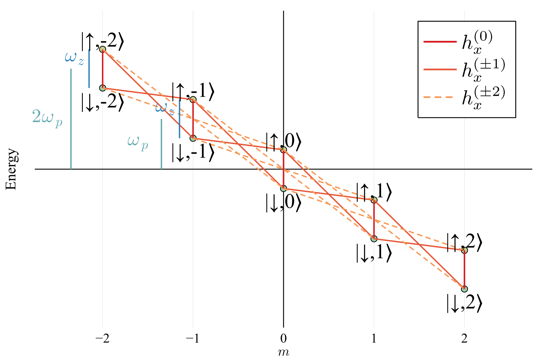
Figure 1: Schematic plot of the Floquet Hamiltonian for a single qubit described by Eq. 3 with $h_{x}(t)=h_{x}(t+\tau)$. Each state is characterized by two quantum numbers: spin ($\uparrow$ or $\downarrow$) and Floquet index ($m$). The vertical lines show the energy scales: the driving frequency, $\omega_{p}=2\pi/\tau$, and the two-level splitting, $\omega_{z}$. The first and second harmonics of the drive $h_{x}^{(\pm 1)}$ and $h_{x}^{(\pm 2)}$ correspond, respectively, to nearest neighbour and next-nearest neighbour couplings.

Aiming at quantum simulations with superconducting qubits, we specifically consider the spin model

$$\hat{H}(t)= -\frac{\hbar\omega_{z}}{2}\hat{\sigma}_{z}+\frac{\hbar h_{x}(t)}{2}\hat{\sigma}_{x},$$ (3)

where $\omega_{z}$ and $h_{x}(t)$ are tunable fields, and $\sigma_{\alpha}$ are Pauli matrices . For $h_{x}(t)=h_{x}(t+\tau)$ one obtains a Floquet Hamiltonian of the form of Eq. 2, with $\hat{H}_{0}=-\hbar\omega_{z}\hat{\sigma}_{z}/2+\hbar h_{x}^{(0)}\hat{\sigma}_{x}/2$ and $\hat{H}^{(m)}=h_{x}^{(m)}\hat{\sigma}^{x}$, where $h_{x}^{(m)}=\tau^{-1}\int_{0}^{\tau}h_{x}(t)e^{im\omega_{p}t}\differential{t}$. This Hamiltonian is equivalent to a two-band Wannier–Stark ladder and is schematically shown in Fig. 1, where, for convenience, we have depicted $\hat{H}^{(m)}$ for $|m|\leq 2$ only. To study long-range hopping models, we introduce a time-dependent drive with a power-law frequency spectrum,

$$h_{x}^{(m)}=\frac{h_{0}}{(1+\absolutevalue{m})^{\alpha}}.$$ (4)

This driving field interpolates between a kicked model at $\alpha=0$ and a weak sinusoidal drive for $\alpha\gg 1$. At intermediate $\alpha$’s, the Fourier transform of Eq. 4 corresponds to periodic kicks with a finite width. The resulting time evolution can be easily computed in two limiting cases: (i) For $\alpha=0$, the time evolution over one period is $U(\tau)=U_{z}U_{x}$, where $U_{z}=\exp(-i\omega_{z}\tau\hat{\sigma}_{z}/2)$ corresponds to the evolution between the kicks and $U_{x}=\exp(-ih_{0}\tau\hat{\sigma}_{x}/2)$ describes the kicks. Note that the same stroboscopic time evolution can be obtained by applying alternatively magnetic fields in the $x$ and $z$ direction for finite times. Such bang-bang[bellman1956bang, viola1998dynamical] protocol and the kicked model are characterized by the same stroboscopic evolution (which is the evolution over an integer number of periods), but lead to a different micromotion (i.e. the intermediate evolution during the time periods). Due to this difference, these two protocols are mapped to different lattice models: the bang-bang protocol corresponds to a short-range hopping model, while the kicked protocol is mapped to a long-range model. (ii) For $\omega_{z}=0$, the Hamiltonian corresponds to a time-dependent magnetic field in the $x$ direction, whose time evolution is $U(t)=\exp(-i\int\differential{t}h_{x}(t)\hat{\sigma}_{x}/2)$.

The driving field of Eq. 4 undergoes a scaling transition between short-range and long-range as a function of $\alpha$. In general, a system is said to be short ranged (or long-ranged) if the integral over space of the coupling is finite (or infinite). In systems with short-range couplings the total energy is extensive (i.e. proportional to the size of the system), while for long-ranged couplings, the total energy grows faster than the system size. See, for example, Refs. [campa2019ising, defenu2020criticality] for the critical properties of this transition, in the context of particles with power-law interactions. In our mapping to a one-dimensional lattice, the Fourier component $h_{x}^{(m)}$ plays the role of the coupling between two sites at distance $m$, see Fig. 1. The system is short/long ranged depending on the finiteness of the sum of $h_{x}^{(m)}$ over $m$, $h_{\mathrm{sum}}=\sum_{m}h_{x}^{(m)}$. In the case of the power-law spectrum introduced in Eq. 4, this quantity diverges for $\alpha<1$. Hence, the system under consideration undergoes a transition between short range and long range at $\alpha=1$.

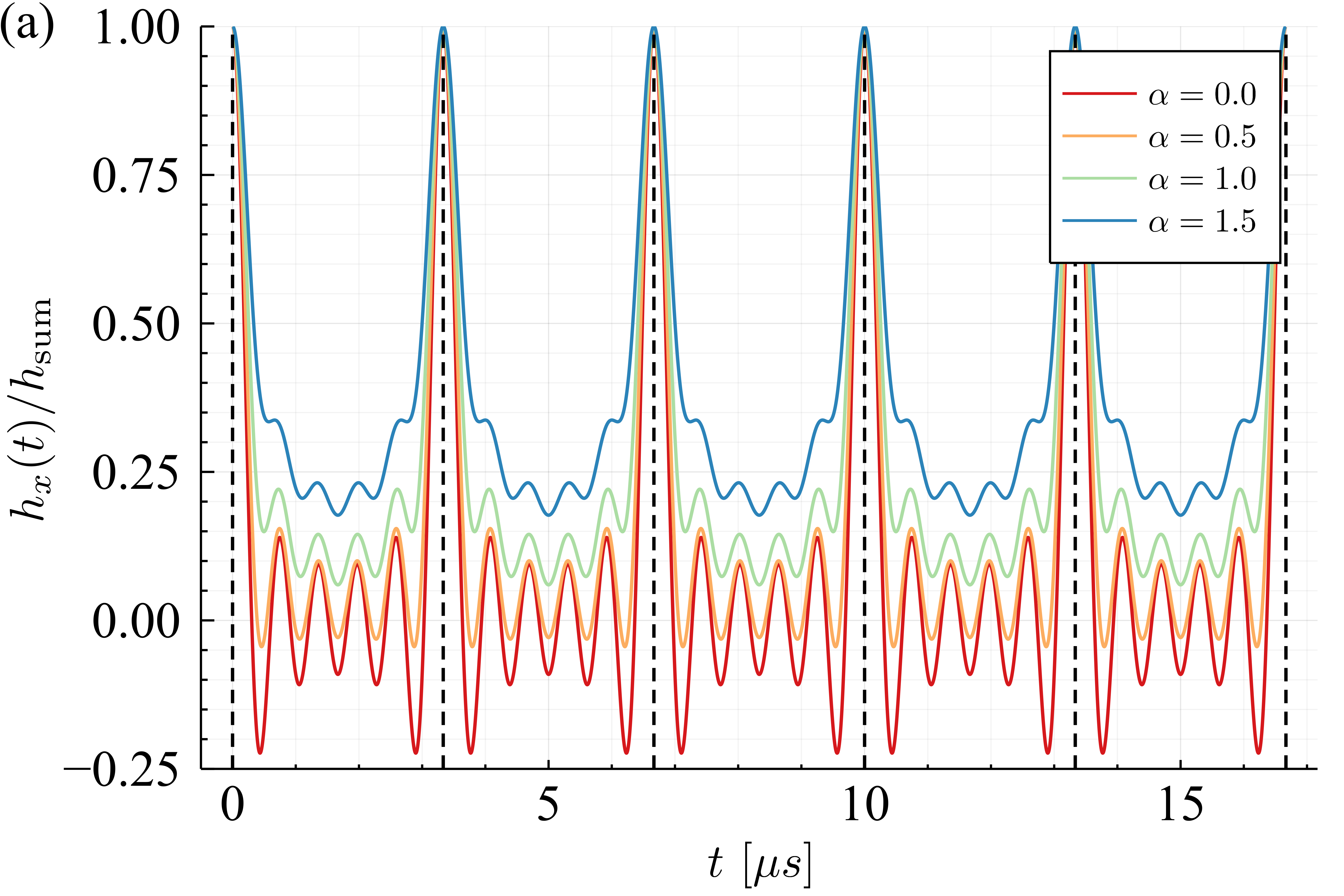
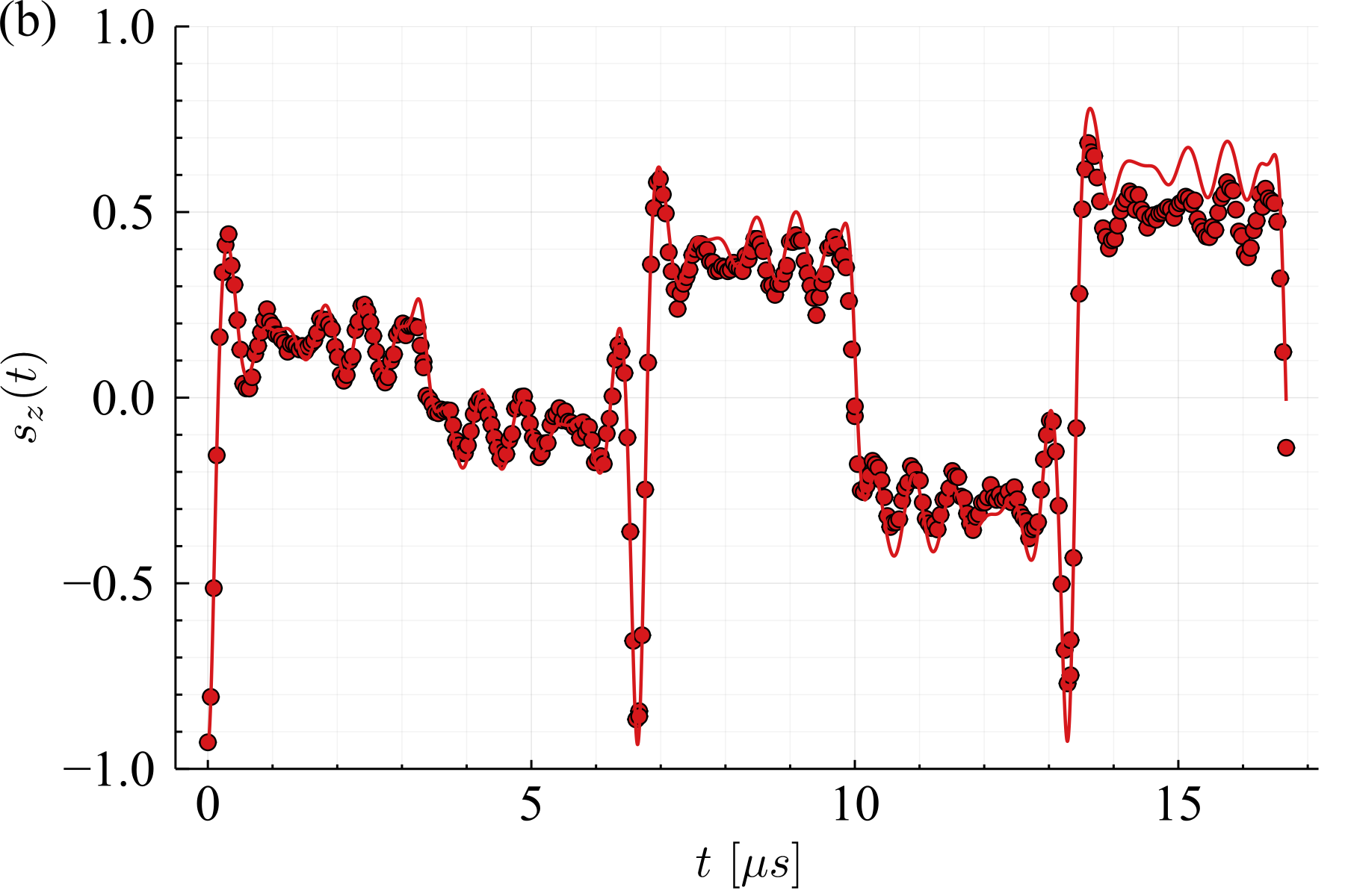
Figure 2: (a) Time-dependent drive with power law spectrum, Eq. 4, with a cutoff at $M=5$, for different values of $\alpha$. (b) Time evolution of the qubit for $M=5$ and $\alpha=0$, theory (lines) and experiment (dots).

In our mapping of periodically driven dynamics to long-range hopping, $h_{\mathrm{sum}}$ corresponds to the effective drive strength at integer multiples of $\tau$, $h_{\mathrm{sum}}=h_{x}(n\tau)$ with integer $n$, which is always finite in a real experiment. To address this problem, we introduce a physical cutoff $M$, by assuming that $h_{x}^{(m)}$ is given by Eq. 4 for all $m\leq M$, and equals 0 for $m>M$. The resulting time dependent drive in shown in Fig. 2(a). As we will see, the cutoff parameter $M$ offers a powerful knob to probe the power-law tails of the Floquet functions.

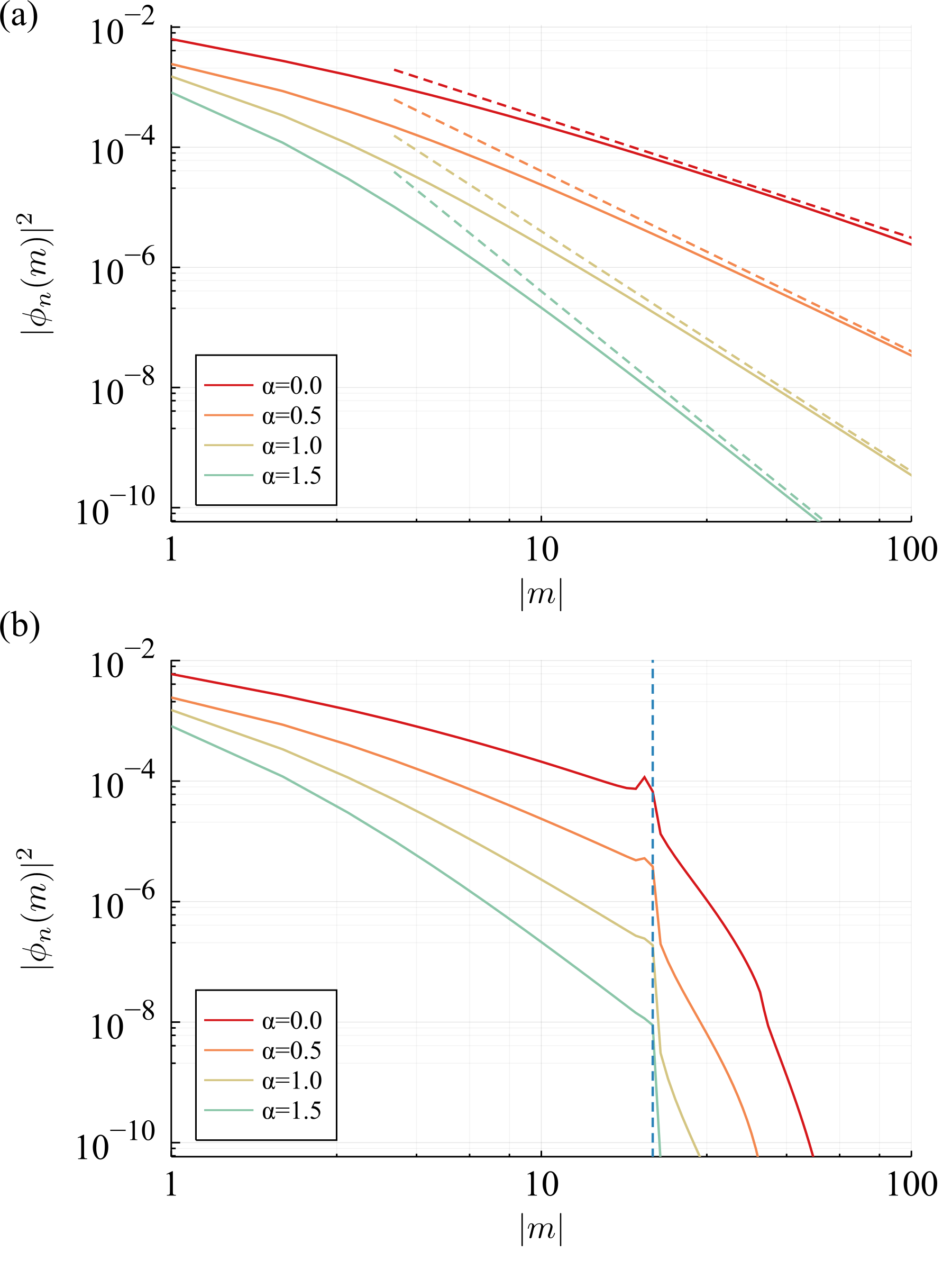
Figure 3: (a) Eigenstate of the Floquet Hamiltonian: numerical diagonalization of $\hat{H}_{F}$ (continuous lines) and power-law asymptotics (dashed lines), Eq. 5. The normalization of the wavefunction is guaranteed by the value of $\absolutevalue{\phi_{n}(m=0)}^{2}$ (not shown). (b) Numerical diagonalization in the presence of a cutoff at $M=20$, giving rise to distinctive peak at $m=M$.

Our experimental setup is a single-qubit quantum computer, available on the cloud, the IBM Quantum processor[ibm2021] ibmq_armonk v2.4.0 which is one of the IBM Quantum Canary processors. The typical physical parameters that we use are $\omega_{z}=2\pi\times$250\text{\,}\mathrm{kHz}$$, $h_{\mathrm{sum}}=2\pi\times$1.2\text{\,}\mathrm{MHz}$$, and $\omega_{p}=2\pi\times$300\text{\,}\mathrm{kHz}$$, or $\tau=$3.3\text{\,}\mathrm{\SIUnitSymbolMicro s}$$. This choice enables us to have $\delta t\ll\tau\ll\min[T_{1},T_{2}]$, where $\delta t=$0.000\,22\text{\,}\mathrm{\SIUnitSymbolMicro s}$$ is the smallest programmable time step and $T_{1}=$160\text{\,}\mathrm{\SIUnitSymbolMicro s}$$ and $T_{2}=$280\text{\,}\mathrm{\SIUnitSymbolMicro s}$$ are the decay and coherence times. In our experiment, we prepare the qubit in the $\ket{\downarrow}$ state, set $\omega_{z}$ to a fixed value, apply the drive $h_{x}(t)$ for time $t$, measure the expectation value $s_{z}(t)=\expectationvalue*{\hat{\sigma}_{z}}$ over 8192 shots, and repeat the procedure for 740 time steps between $t=0$ and $T=5\tau$, see Fig. 2(b).

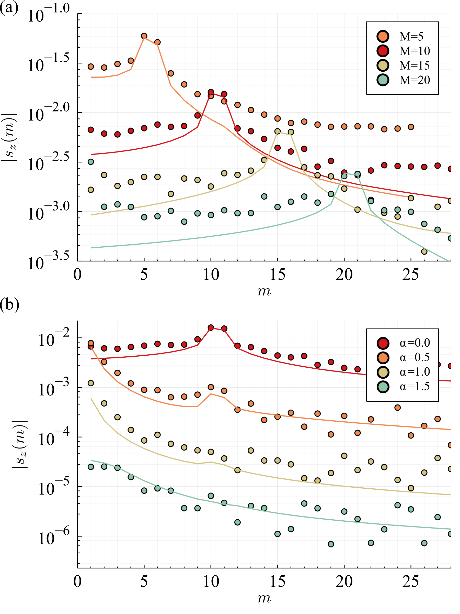
Figure 4: Amplitude of the discrete Fourier components $s_{z}(m)$: theory (lines) and experiment (dots). (a) For different values of $M$ at $\alpha=0$; (b) For different values of $\alpha$ at $M=10$. The pronounced peak at $m=M$ is an indicator of the long-range nature of the Floquet wavefunction (see text). For clarity, the curves with $\alpha>0$ in (b) are shifted vertically by $10^{2\alpha}$.

In the following, we propose and realize two complementary methods to experimentally probe the long-range nature of the model. The first method is based on the power-law scalings of the eigenstates of the enlarged Floquet Hamiltonian $\hat{H}_{F}$. In the absence of a cutoff, the Floquet functions are composed of a central peak at $m=0$ and long power-law tails, $\absolutevalue{{\phi_{n}(m)}}^{2}\sim\absolutevalue{m}^{-x}$, see Fig. 3(a). The value of $x$ can be analytically derived by the following scaling argument: If we consider the product of the $m$^th row of the matrix $\hat{H}_{F}$ with an eigenstate, the central peak gets multiplied by $h_{x}^{(m)}\sim\absolutevalue{m}^{-\alpha}$, while the long tail multiplies the $m$^th diagonal element of $\hat{H}_{F}$, giving rise to a contribution of the order $m^{1-x/2}$. Because the eigenvalue does not depend on $m$, the two contributions needs to scale in the same way and, hence, $x=2+2\alpha$, or

$$\absolutevalue{{\phi_{n}(m)}}^{2}\sim\frac{1}{\absolutevalue{m}^{2+2\alpha}}.$$ (5)

Note that for all $\alpha\geq 0$, one has $\sum_{m}\absolutevalue{\phi_{n}(m)}^{2}<\infty$, ensuring that the Floquet functions $\ket{\phi_{n}(t)}$ are normalizable. In the presence of a cutoff $M$, the Floquet functions decay exponentially for $m>M$, see Fig. 3(b). To preserve the normalization condition, the weight lost at $m\gg M$ appears as a pronounced peak at $m\approx M$. This peak indicates that the Floquet functions are affected by the cutoff only at distances $m\sim M$ and appears sharp on a logarithmic scale. Its integrated weight is proportional to $\sum_{m>M}m^{-2-2\alpha}\approx 1/M^{1+2\alpha}$ and rapidly decreases with $\alpha$. This peak can be experimentally probed by studying the Fourier components $s_{z}(m)=T^{-1}\int_{0}^{T}\differential{t}s_{z}(t)e^{-im\omega_{p}t}$, see Fig. 4. The key feature that we observe is a pronounced peak at $m=M$. This peak is washed out as $\alpha$ increases and becomes invisible at $\alpha>1$, probing the scaling transition at $\alpha=1$.

Our second method to probe the scaling of the Floquet functions relies on the relation between the time derivatives of physical observables and the moments of $\ket{\phi_{n}(m)}$. According to Eq. 1, the $q$^th time derivative of the expectation value of an operator $\hat{O}$ in the state $\ket{\phi_{n}(t)}$, $\pqty{\derivative*{t}}^{q}\expectationvalue*{\hat{O}(t)}_{n}$, equals to

$$(i\omega_{p})^{q}\sum_{m,m^{\prime}}(m-m^{\prime})^{q}\matrixelement{\phi_{n}(m^{\prime})}{\hat{O}}{\phi_{n}(m)}e^{i(m-m^{\prime})\omega_{p}t}.$$

A rigorous bound to this quantity can be obtained by assuming that $\hat{O}$ satisfies $\absolutevalue*{\matrixelement*{\phi_{n}}{\hat{O}}{\phi_{m}}}\leq\norm*{\hat{O}}$, where $\norm*{\hat{O}}$ is the operator norm . This requirement is generically satisfied by operators that act on a finite Hilbert space, such as spin operators, and it does not apply to some operators of a infinite Hilbert space, such as the position or momentum operators of an oscillator, whose matrix elements can be arbitrary large. In this case,

$$\absolutevalue{\derivative[q]{t}\expectationvalue*{\hat{O}(t)}}\leq \omega_{p}^{q}\norm*{\hat{O}}\sum_{\mathchoice{\hbox to0.0pt{$\displaystyle{m,m^{\prime}}$\hss}}{\hbox to0.0pt{$\textstyle{m,m^{\prime}}$\hss}}{\hbox to0.0pt{$\scriptstyle{m,m^{\prime}}$\hss}}{\hbox to0.0pt{$\scriptscriptstyle{m,m^{\prime}}$\hss}}}\absolutevalue{m-m^{\prime}}^{q}\innerproduct{\phi_{n}(m)}{\phi_{n}(m^{\prime})}.$$ (6)

Using the scaling relation of Eq. 5, one can show that the right hand side of Eq. 6 scales as $M^{q-\alpha}$ for large $M$, see appendix B. This expression is finite for $q<\alpha$ and diverges for $q\geq\alpha$. In particular, for the kicked Hamiltonian ($\alpha=0$) the $q=0$ series diverges, highlighting the above-mentioned truncation problem. For all $\alpha\leq 1$, the $q=1$ series diverges, leading to a divergence of the time derivative $\derivative*{t}\expectationvalue*{\hat{O}(t)}$. For larger values of $\alpha$, the $q=1$ series is convergent, but higher-order series (and, hence, higher order derivatives) are infinite. Hence, in our model the time derivatives of physical observables can serve as order parameters of the scaling transition, in analogy to the role of two-point correlation functions for symmetry breaking phase transitions. Figure 5 compares the experimental measurement and numerical calculation of the time derivative of $s_{z}(t)$. The scaling behavior changes drastically at the transition between long-range and short-range couplings ($\alpha=1$). For $\alpha\leq 1$, $\derivative*{s_{z}}{t}\pqty{t=\tau}$ diverges with increasing $M$, while for $\alpha>1$ it saturates to a finite value, in agreement with our scaling argument (see also appendix B).

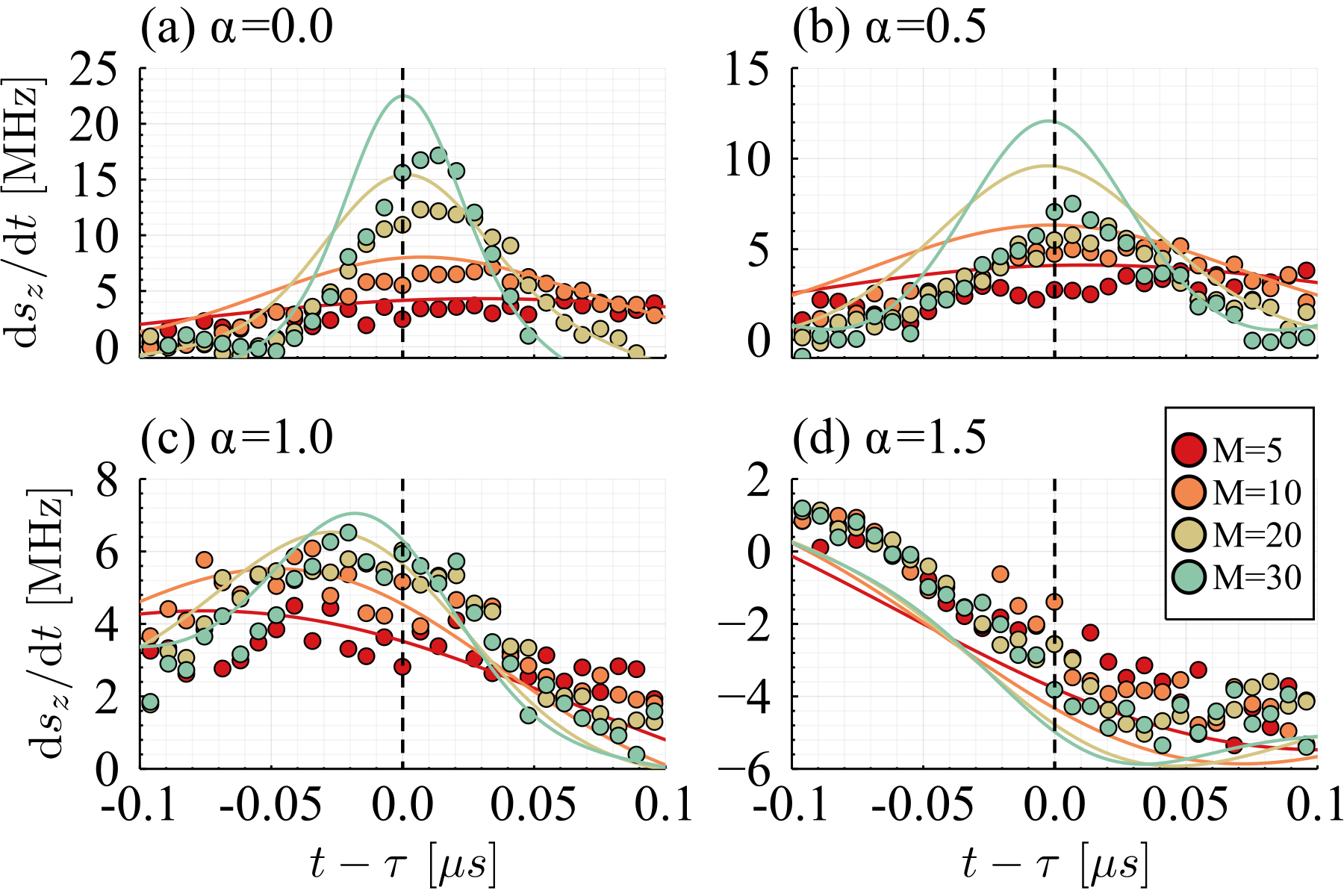
Figure 5: Time evolution of $\derivative*{s_{z}}{t}$ in the vicinity of $t=\tau$: theory (lines) and experiment (dots). The cutoff parameter $M$ allows us to identify the transition between long-range and short-range hopping at $\alpha=1$.

In conclusion, we used Floquet engineering to simulate a one dimensional lattice with power-law hopping. We studied the scaling properties of the Floquet eigenstates and determined the effects of the long tails on the expectation values of physical observables and their time derivatives. By realizing this model on a quantum computer, we demonstrated the experimental capability of controlling and measuring a large number ($M=30$) of harmonics. We were able to probe the long tails of the Floquet functions, both in real time and in Fourier space, and to study their dependence on the exponent $\alpha$. Our experimental observations probe the scaling transition between long-range and short-range couplings.

In recent years, superconducting circuits were used to simulate interesting nonequilibrium effects [bassman2021simulating, bharti2021noisy], including many-body localization of photons [roushan2017spectroscopic] and quench dynamics in one [smith2019simulating] and two [mei2020digital] dimensions. Our work adds an important tool to these simulators, namely pulse engineering for the realization of synthetic Floquet dimensions. Pulse engineering allows us to both realize Floquet Hamiltonians with arbitrary couplings, and to measure the dynamics within each time period, the so called micromotion. By measuring the time harmonic decomposition of the Floquet function, and confirm their scaling properties. Our approach goes beyond previous studies based on stroboscopic measurements, which probe the Floquet quasienergies, but are insensitive to the associated eigenfunctions. By implementing our protocol on a multi-qubit quantum computer, it will be possible to explore equilibrium and nonequilibrium phase transitions with long-range couplings.

Appendix A Quasienergies crossings

In this section we provide a brief analysis of the first Floquet-Brillouin zone of the periodically driven system with long-range interactions with the Floquet Hamiltonian (see Eqs. 2 and 4 in the main text), $\hat{H}_{F}$, and look for any spectral signatures related to the scaling transition. Because we are dealing with a two-level system, the folded spectrum has just two quasienergies. In the extended representation, this pair of quasienergies is repeated every integer multiple of the pump frequency, $\omega_{p}$. Hence, we cannot observe a clustering of states, which is associated with a phase transition, but at most, a level crossing.

We numerically calculated the quasienergies in the first Floquet-Brillouin zone. Typical results of the quasienergies in the folded zone are shown in LABEL:fig:app:der(a)-(c), for different values of $h_{0}$. We, indeed, find that the quasienergies can cross leading to exceptional points of the system. These crossings generically do not occur at $\alpha=1$ and are not related to the transition between long-range and short range couplings discussed in this work.

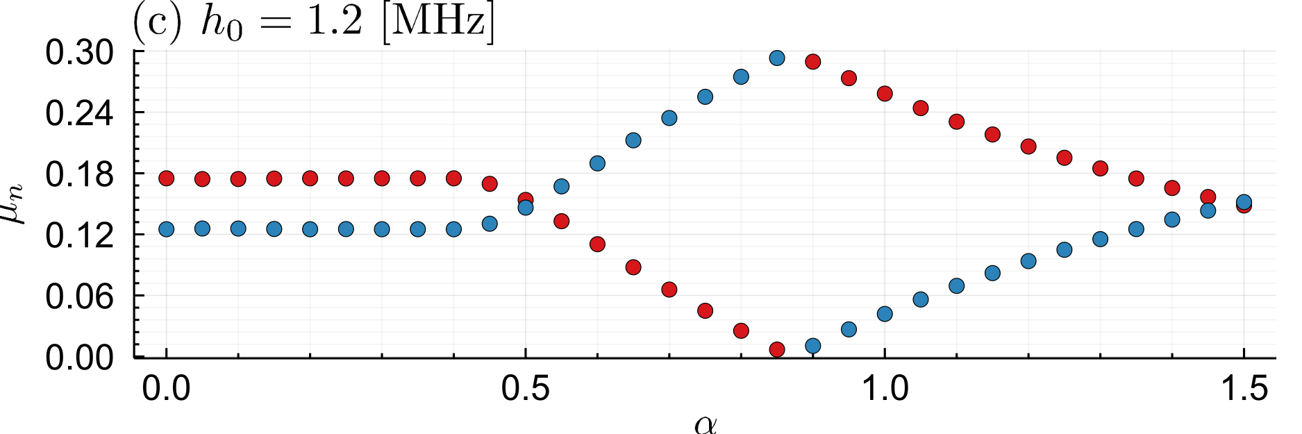
Figure 6: The quasienergies of Eqs. 2 and 5 for various values of the driving strength in the first Floquet-Brillouin zone. Each color represents a different quasienergy.

Appendix B Scaling study of the first derivative of $s_{z}(t)$

This section provides a deeper analysis of theoretical predictions related to Fig. 5 in the main text. In Eq. 6, we have obtained an upper bound for any derivative of generic observables, $\hat{O}(t)$. We will now show how to use the scaling law obtained in Eq. 5 in Eq. 6. We begin by remembering that the eigenfunctions scales as

$$\absolutevalue{\ket{\phi_{n}(m\neq 0)}}\sim \absolutevalue{m}^{-1-\alpha},$$ (7)

$$\absolutevalue{\ket{\phi_{n}(m=0)}}\sim \mathcal{O}(1)$$ (8)

We now separate the sum over $m$ and $m^{\prime}$ in Eq. 6 to two sums, one in which $m$ or $m^{\prime}$ equals zero and another where $m\neq 0$ and $m^{\prime}\neq 0$

$$\sum\limits_{m,m^{\prime}}\to \sum\limits_{\begin{subarray}{c}m,m^{\prime}\\ m\neq 0,m^{\prime}\neq 0\end{subarray}}+\sum\limits_{\begin{subarray}{c}m\\ m^{\prime}=0\end{subarray}},$$ (9)

We, first, consider the double sum with no zeros. For a large cutoff, $M$, we can approximate the double sum to a double integral

$$\sum\limits_{\begin{subarray}{c}m,m^{\prime}\\ m\neq 0,m^{\prime}\neq 0\end{subarray}}\to \iint\limits_{\begin{subarray}{c}m\neq 0\\ m^{\prime}\neq 0\end{subarray}}\differential{m}\differential{m^{\prime}},$$ (10)

using the scaling law of Eq. 7 we can rewrite Eq. 6 as

$$\absolutevalue{\derivative[q]{t}\expectationvalue*{\hat{O}(t)}}\leq\omega_{p}^{q}\norm*{\hat{O}}\\ \times\iint\limits_{\begin{subarray}{c}m\neq 0\\ m^{\prime}\neq 0\end{subarray}}\differential{m}\differential{m^{\prime}}\absolutevalue{m-m^{\prime}}^{q}\absolutevalue{m}^{-1-\alpha}\absolutevalue{m^{\prime}}^{-1-\alpha},$$ (11)

we will examine the scaling of the integral, so we will ignore any numerical constants for the sake of brevity

$$\iint\limits_{\begin{subarray}{c}m\neq 0\\ m^{\prime}\neq 0\end{subarray}}\differential{m}\differential{m^{\prime}}\absolutevalue{m-m^{\prime}}^{q}\absolutevalue{m}^{-1-\alpha}\absolutevalue{m^{\prime}}^{-1-\alpha}\\ \begin{aligned} \\ \sim&\int\limits_{1}^{M}\differential{m}\int\limits_{1}^{m}\differential{m^{\prime}}\pqty{m-m^{\prime}}^{q}m^{-1-\alpha}\pqty{m^{\prime}}^{-1-\alpha}\\ \sim&\int\limits_{1}^{M}\differential{m}\int\limits_{1}^{m}\differential{m^{\prime}}\sum\limits_{k=0}^{q}m^{q-k}\pqty{m^{\prime}}^{k}m^{-1-\alpha}\pqty{m^{\prime}}^{-1-\alpha}\\ \sim&\int\limits_{1}^{M}\differential{m}\int\limits_{1}^{m}\differential{m^{\prime}}\sum\limits_{k=0}^{q}m^{q-k-1-\alpha}\pqty{m^{\prime}}^{k-1-\alpha}\\ \sim&\int\limits_{1}^{M}\differential{m}\sum\limits_{k=0}^{q}m^{q-k-1-\alpha}m^{k-\alpha}\\ \sim&\int\limits_{1}^{M}\differential{m}m^{q-1-2\alpha}.\end{aligned}$$ (12)

At this point we need to preform the integral carefully. If $q=2\alpha$ the integral has a logarithmic behavior. Otherwise, if $q>2\alpha$, the integral scales as $M^{q-2\alpha}$ or saturates to a finite values of order ine if $q<2\alpha$. Hence, we find

$$\iint\limits_{\begin{subarray}{c}m\neq 0\\ m^{\prime}\neq 0\end{subarray}}\differential{m}\differential{m^{\prime}}\absolutevalue{m-m^{\prime}}^{q}\absolutevalue{m}^{-1-\alpha}\absolutevalue{m^{\prime}}^{-1-\alpha}\\ \sim\begin{cases}\ln(M),&q=2\alpha,\\ M^{q-2\alpha},&q>2\alpha,\\ 1,&q\leq 2\alpha.\end{cases}.$$ (13)

Now we will focus on the sum in which either $m$ or $m^{\prime}$ equals zero. As before, we convert the sum into an integral

$$\sum\limits_{\begin{subarray}{c}m\\ m^{\prime}=0\end{subarray}}\to \int\limits_{1}^{M}\differential{m},$$ (14)

plugging in the scaling law of Eq. 8 we rewrite Eq. 6

$$\begin{split}\int\limits_{1}^{M}\differential{m}\absolutevalue{m}^{-1-\alpha}\absolutevalue{m}^{q}\sim&\int\limits_{1}^{M}\differential{m}\pqty{m}^{q-1-\alpha}.\end{split}$$ (16)

Just like before, we need to preform the integral carefully. If $q=\alpha$ the integral has a logarithmic behavior. Otherwise, if $q>\alpha$ the integral scales as $M^{q-\alpha}$, or scales as 1 if $q<\alpha$.

$$\int\limits_{1}^{M}\differential{m}\absolutevalue{m}^{-1-\alpha}\absolutevalue{m}^{q}\sim \begin{cases}\ln(M),&q=\alpha,\\ M^{q-\alpha},&q>\alpha,\\ 1,&q\leq\alpha.\end{cases}.$$ (17)

Using Eqs. 9, 13 and 17 we can deduce the leading behavior of Eq. 6 presented in the text

(18)