The TW Hya Rosetta Stone Project IV: A hydrocarbon rich disk atmosphere

Abstract

Connecting the composition of planet-forming disks with that of gas giant exoplanet atmospheres, in particular through C/O ratios, is one of the key goals of disk chemistry. Small hydrocarbons like $\rm C_{2}H$ and $\rm C_{3}H_{2}$ have been identified as tracers of C/O, as they form abundantly under high C/O conditions. We present resolved $c-$C₃H₂ observations from the TW Hya Rosetta Stone Project, a program designed to map the chemistry of common molecules at $15-20$ au resolution in the TW Hya disk. Augmented by archival data, these observations comprise the most extensive multi-line set for disks of both ortho and para spin isomers spanning a wide range of energies, $E_{u}=29-97$ K. We find the ortho-to-para ratio of $c-$C₃H₂ is consistent with 3 throughout extent of the emission, and the total abundance of both $c-$C₃H₂ isomers is $(7.5-10)\times 10^{-11}$ per H atom, or $1-10$% of the previously published $\rm C_{2}H$ abundance in the same source. We find $c-$C₃H₂ comes from a layer near the surface that extends no deeper than $z/r=0.25$. Our observations are consistent with substantial radial variation in gas-phase C/O in TW Hya, with a sharp increase outside $\sim 30$ au. Even if we are not directly tracing the midplane, if planets accrete from the surface via, e.g., meridonial flows, then such a change should be imprinted on forming planets. Perhaps interestingly, the HR 8799 planetary system also shows an increasing gradient in its giant planets’ atmospheric C/O ratios. While these stars are quite different, hydrocarbon rings in disks are common, and therefore our results are consistent with the young planets of HR 8799 still bearing the imprint of their parent disk’s volatile chemistry.

1 Introduction

We are entering an era where measurements of the compositions of giant exoplanet atmospheres are becoming increasingly common. A diversity of chemical properties (via carbon-to-oxygen ratios, or C/O) has been seen (e.g., Madhusudhan et al., 2011; Madhusudhan, 2012; Kreidberg et al., 2015), including within a single planetary system (HR8799; Bonnefoy et al., 2016; Lavie et al., 2017; Lacour et al., 2019; Mollière et al., 2020). To understand the origins of this diversity, we must study planets’ formation environments: gas rich protoplanetary disks. The chemical properties of these disks are driven by at least two factors, i. the make-up of the molecular cloud out of which the star and disk formed (e.g., Visser et al., 2009, 2011; Drozdovskaya et al., 2019), and ii. the disk physical properties (irradiation level, temperature, density, etc.) that can drive an actively evolving chemistry prior to and during planet formation (e.g., Cleeves et al., 2014).

The relative contribution of these factors, i.e., the role of inheritance versus later chemical reprocessing in the disk itself, changes with both radial and vertical location. For example, near the highly irradiated disk surface and/or close to the central star, the chemistry is effectively “scrambled” leaving little memory of the molecular composition of the cloud. Near the midplane, especially in the outer disk (beyond $\sim 10$ au), the high extinction levels provide a safer haven for some of the material originating in the molecular cloud to be preserved, with further processing requiring moderate to high external irradiation or cosmic ray fluxes (e.g., Bergin et al., 2014; Cleeves et al., 2014; Yu et al., 2017; Eistrup et al., 2018); however, it is unclear whether disks are sufficiently ionized to facilitate an active midplane chemistry (Cleeves et al., 2015).

There is a growing body of evidence that the observable chemistry in planet forming disks, at least that within the “warm molecular layer” (Aikawa et al., 2002), deviates from “typical” molecular cloud chemistry. For example, observations of CO emission and CO isotopologues are faint when compared to expectations based on dust masses from millimeter emission, a gas-to-dust correction factor, and an interstellar CO abundance (e.g., Favre et al., 2015; Schwarz et al., 2016; Ansdell et al., 2016). Water was surprisingly challenging to detect in protoplanetary disks with Herschel, and when detected, fluxes were more than an order of magnitude lower than anticipated based on astrochemical modeling with UV irradiated water ice at interstellar abundances (Bergin et al., 2010; Hogerheijde et al., 2011; Du et al., 2017). The abundant interstellar complex organic methanol, first detected in disks by the Atacama Large Millimeter Array (ALMA), was similarly quite faint (Walsh et al., 2014), yet observations of CH₃CN appeared relatively bright, with nearly a 1:1 abundance ratio inferred between them for the TW Hya disk (Loomis et al., 2018).

Therefore we need better constraints on the chemical composition of disk gas, especially at an elemental level, to understand the chemical reservoir from which planets may accrete and what, e.g., C/O or N/O ratio they might inherit at least initially. Chemical models have demonstrated that the abundances of simple hydrocarbons like C₂H and $c-$C₃H₂ are very sensitive to the C/O ratio of the gas (e.g., Bergin et al., 2016; Kama et al., 2016; Cleeves et al., 2018; Miotello et al., 2019; Fedele & Favre, 2020). Pure freeze-out of solids from gas can vary C/O in the gas or ice from $\sim 0.2$ to 1 (Öberg et al., 2011) around the conventional solar value of 0.54. Cleeves et al. (2018) found that the abundance of C₂H was extremely sensitive to the bulk C/O in volatiles until C/O $>1$ (ratios of 1.9 and 3.7 were indistinguishable in their models; see also Bosman et al. (2021)). Therefore, hydrocarbons are expected to be a useful tool for estimating C/O up to $\sim 1.5$, which overlaps with observed exoplanet atmospheric values. As a result, disk hydrocarbon studies open an exciting potential avenue to connect the composition of the gas in disks to that measured in planets’ atmospheres. In addition, observations of hydrocarbon emission in disks have been found to be generally quite bright at sub-mm wavelengths (Qi et al., 2013a; Kastner et al., 2014, 2015; Bergin et al., 2016; Cleeves et al., 2018; Bergner et al., 2019), enabling small surveys ($\lesssim 14$ sources) of C₂H emission in disks (Guilloteau et al., 2016; Miotello et al., 2019; Bergner et al., 2019).

The next step is localizing the distribution of hydrocarbons in the disk, to understand the range of possible C/O values a planet could inherit from a single disk environment. The first resolved image of C₂H was made of the TW Hya disk by Kastner et al. (2015) with the Submillimeter Array, where it was found to have a ring-like morphology. Its disk-averaged physical nature was constrained using multiple transitions and its hyperfine structure. However, due to the face-on nature of this disk $5-7^{\circ}$ (Qi et al., 2006, 2008; Huang et al., 2018), degenerate excitation solutions were found to fit the data, either a cold, dense solution or alternatively a relatively warmer, but low density solution. The former would suggest an enhanced (greater than solar) C/O ratio fairly deep into the disk gas, near the planet-forming region, while the latter would suggest that the C/O enhancement primarily is closer to the surface and perhaps less connected to the planet forming midplane.

Bergin et al. (2016) presented further resolved observations confirming C₂H’s ring-like geometry, as well as observations of $c-$C₃H₂ toward TW Hya. The spatial distribution of C₂H and $c-$C₃H₂ were found to match identically in radial distribution, suggestive that this radial region of the TW Hya disk supports a generally rich hydrocarbon chemistry, consistent with an elevated C/O ratio in this region.

The present paper uses multi-line observations of $c-$C₃H₂ to better spatially constrain the nature of the hydrocarbon layer in the TW Hya protoplanetary disk, with the goal of improving our interpretation of the C/O ratio(s) of this disk. The observations were conducted as part of the TW Hya as a Chemical Rosetta Stone Project (PI: Cleeves), and have been augmented with ALMA archival data. The set of lines covers energies spanning 29.1 K to 96.5 K, and with the relatively highly critical density and range of opacities probed, these lines are well suited to constraining the nature, and crucially the location, of small hydrocarbon chemistry in TW Hya.

2 Observations

2.1 ALMA Observations

Table 1: $c-$C₃H₂ Observations

Line	o or p	$\nu$	$A_{ij}$	Eu	Channel width	rms	Int. flux	Program
		(GHz)	(s-1)	(K)	(km/s)	(mJy/beam)	(mJy km/s)
$4_{3,2}-3_{2,1}$	o	227.16913	3.113E-04	29.07	0.16	3.2	$80\pm 5$	1
$7_{3,4}-6_{4,3}$	o	351.52327	1.237E-03	77.24	0.21	3.4	$237\pm 13$	2
$8_{3,6}-7_{2,5}$	o	352.19364	1.734E-03	86.93	0.21	4.2	$220\pm 30$	3
$5_{5,1}-4_{4,0}$	p	338.20399	1.598E-03	48.78	0.21	5.3	$140\pm 16$	3
$8_{2,6}-7_{3,5}$	p	352.18551	1.735E-03	86.93	0.21	4.3	$96\pm 15$	3
$9_{1,8}-8_{2,7}$	o (bl)	351.96593	2.117E-03	93.34	0.21	2.9	$398\pm 14$	2,3
$9_{2,8}-8_{1,7}$	p (bl)	351.96594	2.117E-03	93.34
$10_{1,10}-9_{0,9}$	o (bl)	351.78157	2.439E-03	96.50	0.21	2.9	$330\pm 15$	2,3
$10_{0,10}-9_{1,9}$	p (bl)	351.78157	2.439E-03	96.50

The observations of $c-$C₃H₂ utilized in the present study were carried out with ALMA as part of three different observational programs. We present new observations of $c-$C₃H₂ taken as part of the TW Hya as a Chemical Rosetta Stone Program (PI: Cleeves, 2016.1.00311.S), augmented by archival observations from 2013.1.00198.S (PI: Bergin) and 2013.1.00114.S (PI: Öberg). The complete set of $c-$C₃H₂ transitions from these programs used in our analysis are listed in Table 1. The observations from 2016.1.00311.S were carried out with 40 antennas on April 8, 2017 (C40-2; 15m – 390m baselines) and May 21, 2017 (C40-5; 15m – 1124m baselines). The April 8 observation used J1037-2934 for bandpass and phase calibration, and J1058+0133 for flux calibration. The May 21 observation used J1037-2934 for bandpass, flux, and phase calibration.

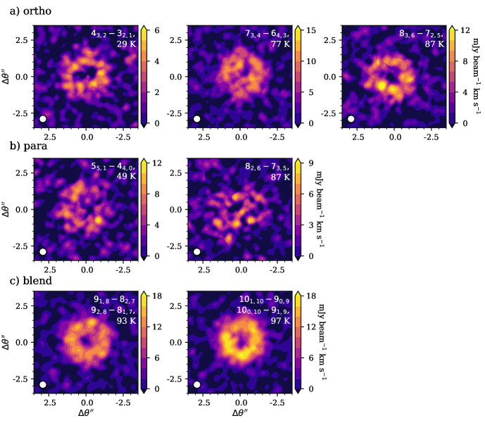
Figure 1: Moment zero maps for the five isolated transitions of a) ortho, b) para, and c) two blended transitions of $c-$C₃H₂ that are analyzed in this work. Line ID and upper state energy are labelled in the upper right corner of each panel.

All data were calibrated with the ALMA pipeline with CASA version 4.7.0. Prior to imaging, we phase self-calibrated the data using the line-free portions of the continuum, adopting a solution interval of 30s and averaging polarizations. In addition, spws were self calibrated independently, and we set a minimum signal to noise ratio of 3 and a minimum number of baselines per antenna of 6. The calibration process for the observations from program 2013.1.00198.S and 2013.1.00114.S are reported in Bergin et al. (2016) and Öberg et al. (2017) and not repeated here.

The projects 2013.1.00198.S and 2016.1.00311.S had overlapping coverage of the bright 10 – 9 and 9 – 8 blends (see Table 1). The integrated line flux measured between these two programs differed by about 10% (well within the quoted ALMA flux uncertainty), however we adjusted the flux of 2013.1.00198.S to match the flux measured in 2016.1.00311.S flux. As a result, 6 of the 7 lines have internally consistent fluxes, and therefore RMS uncertainties reported here do not include flux calibration uncertainty, as that will either net increase/decrease measured flux but will not impact the spatially resolved shape of the line images.

2.2 Images and Radial Integrated Flux Profiles

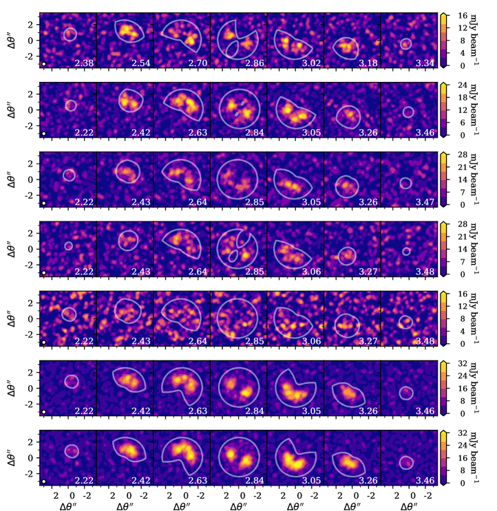
Figure 8: Channel maps for the transitions of $c-$C₃H₂ observed, where o = ortho, p = para, and b = blend. The contour indicates the Keplerian mask used for cleaning and for the measurements of the fluxes presented in Table 1.

The continuum was subtracted in the uv-plane using the CASA task uvcontsub assuming a linear fit to the continuum shape. Imaging was carried out using the tclean task in a semi-automated fashion described here. The source velocity was assumed to be 2.84 km s^-1. For each line, using all available data for a given transition, we begin by creating a dirty image to determine the standard deviation per beam in line free channels and the beam size for each transition. From these data, we create a mask based on expectations from Keplerian motion using the code presented as part of Pegues et al. (2020), see also code reference jpegues (2020). We assume an inclination of $5^{\circ}$, a position angle of $152^{\circ}$, and a stellar mass of 0.8 M_⊙ to create the Keplerian mask following Huang et al. (2018). We assume a distance of 59.5 pc (Gaia Collaboration et al., 2016). The mask is convolved with the respective beam for each data set (typically between $0\farcs 2-0\farcs 4$). Because we want to have a consistent beam size across all the transitions, which we chose to be $0\farcs 5$, we calculate the uv-taper that is necessary to create a beam of just below $0\farcs 5$ on the major axis. We then clean each line with its respective mask in non-interactive mode down to a noise level of 3$\sigma$ standard deviation, with the line specific uv-taper applied. Finally, we take the cleaned image and apply the CASA task imsmooth, which operates in the image plane, to create a final image with an exactly $0\farcs 5$ round beam. The result of this imaging process is shown in Figure 1. The corresponding channel maps for all transitions are also provided in Appendix A, Figure 8.

The ring-like nature of the emission is clear from the moment-0 maps, and the general faintness of the para transitions compared to the ortho transitions is also clear. We do not use these moment-0 maps for analysis, showing them here to illustrate the detection significance, and instead we apply the GoFish package (Teague, 2019) to improve the signal to noise of the radial profile for each transition. GoFish works in the image plane to spectrally align spectra at a given radius by taking into account the projected disk rotation, such that the spectra can be stacked, thereby creating a higher signal-to-noise ratio radial intensity profile. We assume the same disk parameters as for the Keplerian masking above to carry out the GoFish deprojection. The deprojection is done on the cleaned image cubes produced with the method described above, and the output is a spectrum at each radius where the width of the emission is some combination of the thermal width and any non-thermal broadening or beam convolution broadening, since Keplerian motion has been accounted for. After shifting and stacking the azimuthal emission, we integrate over a conservative velocity range of 2.5 km s^-1 to 3.18 km s^-1 and obtain the profiles shown in Figure 2. Note that even though the para transitions are faint in the moment-0 maps in Figure 1, the ring-like structure becomes clearer in the GoFish extraction and the peak of the resolved profile is detected at $\geq 3-4\sigma$.

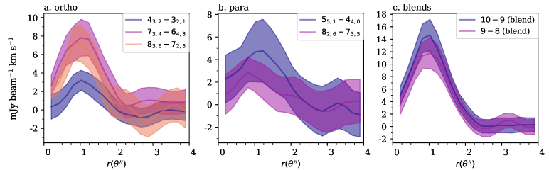
Figure 2: Profiles extracted by the pixel stacking technique within the GoFish code (Teague, 2019). Transitions indicated in the legend. Shaded region indicates the error on the radial profile.

3 Methods

From this multi-line data set of $c-$C₃H₂ rotational transitions spanning upper state energies from 29.1 K to 96.5 K, we aim to use excitation to constrain the location of the hydrocarbon layer in the TW Hya disk. To fit the data, we use a simple slab model method (see e.g., Qi et al., 2008; Öberg et al., 2017) and employ a non-LTE line radiative transfer code based upon Ratran (Hogerheijde & van der Tak, 2000, Astrophysics Source Code Library, record 0008.002) designed to handle blended transitions and be computationally efficient (https://github.com/ryanaloomis/nLTErt1d). The inputs to this code are height ($z$), gas volumetric density, dust density, gas temperature, dust temperature, non-thermal line width, and abundance relative to hydrogen of the molecule of interest.

We approximate the emission from TW Hya as a series of radial annular regions, where the physical conditions as a function of height at each radial location are taken from the Cleeves et al. (2015) model of TW Hya. The gas temperature, dust temperature, and gas density are taken from this model, where the total mass of this TW Hya disk model is 0.04 $M_{\odot}$.

The “slab” $c-$C₃H₂ distribution is bounded by an inner and outer radius, and a vertically computed upper and lower column density of H, $N_{\rm H_{2}}$. Note that for the ISM, $N_{\rm H_{2}}=1.9\times 10^{21}$ cm${}^{-2}=1~{}A_{V}$. But since our model has 6.7$\times$ less small grains in the surface of the disk due to the formation and subsequent settling of larger grains, then $1~{}A_{V}$ occurs at $N_{\rm H_{2}}=1.27\times 10^{22}$ cm^-2. The general reasoning for this vertical parameterization rather than a simple $z/r$ cut is that we expect the $c-$C₃H₂ distribution to be driven by the stellar radiation field, largely UV (Du et al., 2015; Bergin et al., 2016). The abundance is set to a constant value within this “slab,” where we vary the value of this constant. The underlying physical structure and the calculated $N_{\rm H_{2}}$ contours bounding the $c-$C₃H₂ distribution are shown in Figure 3. As can be seen in the right-hand panel, the slabs closer to the disk surface are dominated by warmer temperatures, while deeper in (higher $N_{\rm H_{2}}$) the gas temperatures decrease.

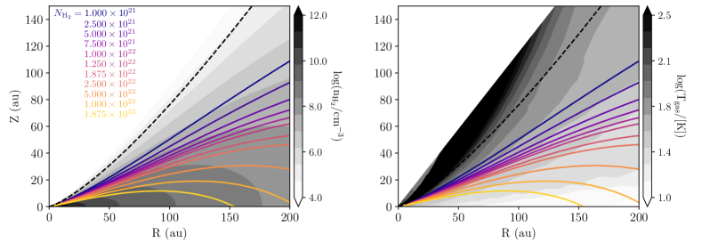
Figure 3: Slab $c-$C₃H₂ model definitions. The vertical extent of $c-$C₃H₂ is described by the vertically integrated column density derived from the Cleeves et al. (2015) TW Hya model shown in grey shaded contours. The upper limit for all models is $N_{\rm H_{2}}=10^{19}$ cm^-2 (dashed line). The bottom of the $c-$C₃H₂ slab is described by the color line contours as labelled in the left panel. The inner and outer radius parameters truncate these boundaries vertically, and the abundance is assumed to be constant inside of the layer.

In addition to the four parameters described above, we also fit for the ortho to para ratio of $c-$C₃H₂, where as can be seen in Table 1 our data set contains both spin isomers and two blended pairs of ortho and para transitions (the brightest lines). We adopt the collisional rate coefficients hosted on the Leiden LAMDA database (Schöier et al., 2005) originally computed in Chandra & Kegel (2000) for ortho and para separately. For the blended transitions, the components of the blends had identical molecular parameters (e.g., Einstein A coefficients, near identical frequencies), and therefore we simulated emission for the blends by first estimating the level populations for each of the ortho and para components independently (while we did not impose it on the solution, the emission was seen to be largely in LTE). We then took a weighted average of the ortho and para populations in the upper and lower states respectively (the population fractions were the same for both spin isomers). This allowed us to simulate the blended $c-$C₃H₂ emission as that from a “single” molecule. We took this approach since for some of the models the blended transitions became optically thick, so we could not simply sum the line fluxes from the independent components without potentially overestimating the blended line flux.

Table 2: Slab Model Parameters

Parameter	Values	Unit
Min H2 Column	$10^{19}$	cm-2
Max H2 Column ($\times 10^{21}$)	1, 2.5, 5, 7.5,	cm-2
	10, 12.5, 18.75, 25,
	50, 100, 187.5
$\chi$($c-$C3H2) ($\times 10^{-11}$)	1, 1.875, 3.75, 5,	per H
	7.5, 10, 25, 50, 75,
	100, 250, 500, $10^{3}$
OPR	1, 3	n/a
$R_{\rm inner}$ $c-$C3H2	20, 25, 30, 35, 40	au
$R_{\rm outer}$ $c-$C3H2	80, 90, 100, 110, 120	au
Total number of models	7150

To create the synthetic integrated radial intensity profile for each model, we reconstruct a 2D sky image of the velocity integrated line brightness and convolve the image with a Gaussian $0\farcs 5$ beam. The use of the larger beam was primarily to be able to circularize and homogenize the beam for all lines in the sample and to improve the signal to noise per beam. We then extract the convolved radial brightness profile in annuli with the same spacing as the GoFish intensity profile.

Goodness of fit is assessed based on a reduced $\chi^{2}$ between the beam-convolved model spectrally integrated intensity profile and the data. To estimate $\chi^{2}$, the flux in a given annulus for the data and model are measured per beam, and we sum the square of the difference divided by the observed RMS uncertainty. The number of annuli super samples the beam but is divided out by the reduced $\chi^{2}$. All lines are treated equally in our overall assessment of fit for a given set of slab model parameters, even though some lines are brighter than others. We made this decision since the brighter lines are optically thick blended transitions, and the lower SNR profiles provide important constraints on our fit. Note, we only consider the RMS uncertainty in this estimate and do not include flux calibration error since eight out of nine lines have self-consistent fluxes, such that flux uncertainty will globally shift all radial line profiles upwards or downwards rather than expanding the error bars uniformly. The only exception is the ortho $c-$C₃H₂ line $4_{3,2}-3_{2,1}$. We therefore have also examined our best fit models from the profiles as extracted directly from GoFish, and then with a 10% uniform increase and decrease on just the $4_{3,2}-3_{2,1}$, with the rest of the lines fixed. We do not find a change in the best fit models, in part since we have two other ortho lines. Furthermore, the models that fit the rest of the data give reasonable fits to the native $4_{3,2}-3_{2,1}$ observations without flux scaling, and therefore we do not vary the flux for the remainder of the analysis described here.

Initially, we also varied the minimum column density of the layer, but since we did not see a significant change between changing the upper boundary from $N_{\rm H_{2}}=1\times 10^{19}$ cm^-2 to $1\times 10^{20}$ cm^-2, we decided to fix the upper boundary for the full grid of simulations to the former value of $1\times 10^{19}$ cm^-2, which for the reduced dust atmosphere corresponds to an $A_{V}$ of 0.0008, i.e., very high up in the atmosphere, where the H₂ gas density is also very tenuous ($\sim 10^{5}$ cm^-3). Thus very little $c-$C₃H₂ in this layer contributes to the emission. The full set of parameters and their values considered in the simulation grid are provided in Table 2. Essentially, each model varies the inner and outer extent, lower layer extent via the column density, the abundance within the layer, and the ortho-to-para ratio of $c-$C₃H₂. The range of values was explored is based on a combination of previous modeling results (e.g., Bergin et al., 2016) along with making sure we explored a wide space around regions that gave better fits to assess degeneracies in the parameter space.

4 Results

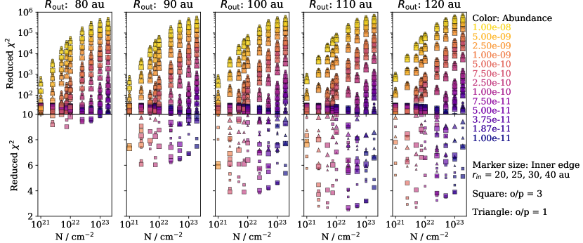
Figure 4: Reduced $\chi^{2}$ between the observed visibilities and modelled visibilities. Each point represents the model fit for all observed lines as a summed reduced $\chi^{2}$. The model parameters are described by the point color (abundance), size (inner radius of $c-$C₃H₂), and shape (ortho to para ratio). The columns indicate different outer radii for the $c-$C₃H₂ slab, for the full range of H₂ column densities considered on each x-axis. The poor fits are shown on a logarithmic scale on the top row, while the better fits are shown as a linear scale on the bottom row.

4.1 Fiducial Model Results

A comparison between all of the 7,150 models in our grid and all observed transitions is illustrated in Figure 4. Each point represents $\chi^{2}_{\rm reduced}$ for all observed lines simultaneously. Due to the large dynamic range across the model grid, we have split each panel into a top and bottom panel where the top row has log scale $\chi^{2}_{\rm reduced}$ and the bottom row shows the same data but with a linear scale for clarity. The best fit models (those with the lowest $\chi^{2}_{\rm reduced}$) are those that appear on the bottom row. From Figure 4, a few key features become clear, and are enumerated here:

1. The models that agree the best with the data have the outer edge of the $c-$C₃H₂ emission at $>100$ au.

2. None of the other parameters in our grid can be tuned to achieve a model with a good fit with an outer edge at $<100$ au.

3. An inner edge of 25 and 30 au tends to be a better fit for the $c-$C₃H₂ distribution. We note that this edge is close to the half-beam of the data (0$\farcs$25 = 15 au), and so cannot constrain this any further from existing data. We also note that the $c-$C₃H₂ “empty” inner disk model is consistent with the non-zero flux near the star seen in our radial profile due to beam convolution effects. Finally, we note that both the value for the inner and outer edge only hold if a slab model is an adequate representation of the data, and certainly more complex structural representations could be explored with higher SNR data.

4. The flatness of the $\chi^{2}_{\rm reduced}$ for the best models suggests some degeneracy between the maximum column density, i.e., the depth of the layer, and the abundance of $c-$C₃H₂ in the layer, which is to be expected especially if the emission is thermalized.

5. While the observations suggest the $c-$C₃H₂ originates in a region of sufficiently high gas density to be thermalized, we can further constrain the vertical location of the $c-$C₃H₂ layer by taking advantage of the wide span of upper state energies in our data set. We can rule out $c-$C₃H₂ emitting from the upper surface (i.e., $N_{\rm H_{2}}\leq 10^{21}$ cm^-2) or from the midplane, below $N_{\rm H_{2}}\geq 10^{23}$ cm^-2. These column densities translate to $A_{V}\leq 0.05$ and $A_{V}\geq 5$, respectively, due to the dust-poor gas in the disk surface.

6. There are no good fits that have an ortho-to-para ratio of $c-$C₃H₂ of 1. Ortho-to-para of 3 is strongly favored over 1. We do not try to fit between these values given the signal to noise of the data.

To provide an even clearer picture of our best fit models, we extract the 30 models with the lowest $\chi^{2}$ from our grid and plot a histogram of the model parameters (see Figure 5). We also plot the radial intensity profiles of these models in Figure 6. Based on this sub-selection of models, an inner radius of 25 or 30 au is favored by 2/3 of the 30 models. Nearly all of the best fit models have an outer radius of $c-$C₃H₂ at $>100$ au, with 110 au favored slightly over 120 au. While there is some degeneracy between the depth of the slab measured by $N_{\rm max}$ and the abundance per H of $c-$C₃H₂, it is clear that models with $N_{\rm max}$ of $(1-3)\times 10^{22}$ cm^-2 are favored by most. The abundance of $c-$C₃H₂ in the slab is between $(3-30)\times 10^{-11}$ per H atom. To test how much of the spread is due to the degeneracy between the thickness of the layer and the abundance, we also show in Figure 5 a histogram of the product of $\chi_{\rm c-C_{3}H_{2}}$ and $N_{\rm max}$ and find that this distribution is much tighter, and corresponds to an approximate column density of $c-$C₃H₂ in the slab of $(1-3)\times 10^{12}$ cm^-2.

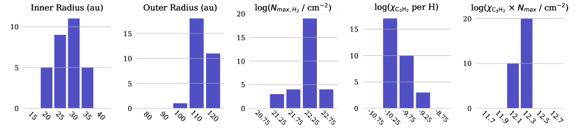
Figure 5: Histogram of the parameters of the 30 best fit models. Note 1 $A_{\rm V}$ Corresponds to $N_{\rm H_{2}}=1.27\times 10^{22}$ cm^-2 given the reduced dust in the upper layers of TW Hya.

The 30 best fit models are shown in Figure 6 in dark grey, and we have additionally highlighted the four best fit models in color and provided their physical parameters in the key. Note all 30 models have an ortho to para ratio of 3, so that parameter is not listed in the figure. The best fit models have similar characteristics, and abundance of $(7.5-10)\times 10^{-11}$ per H atom, and extend down to an H₂ column density of approximately $2\pm 0.5\times 10^{22}$ cm^-2. This depth corresponds to a vertically integrated $A_{V}$ of about 1 due to the reduced small dust mass in the disk upper layers in the Cleeves et al. (2015) TW Hya model.

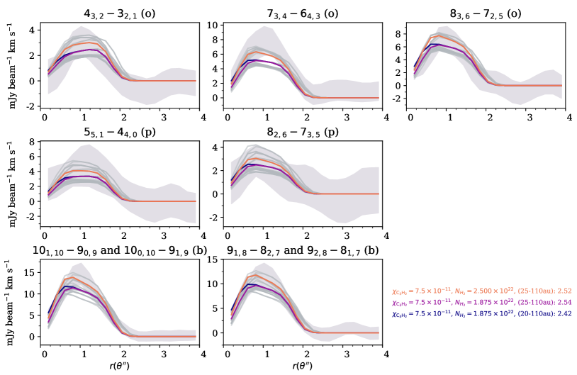
Figure 6: Radial profiles of the integrated emission from each transition, including error bars (shaded gray). Profiles extracted using GoFish. The thirty best fit models are show as gray lines, while the top three models are shown in color, and have parameters indicated in the legend in the lower right-hand corner.

5 Discussion

We have carried out a resolved, multi-line study of hydrocarbon emission in the TW Hya disk as traced by $c-$C₃H₂. The observations span a wide range of upper state energy from 29 K to 96.5 K, and include both ortho and para forms of $c-$C₃H₂. Hydrocarbons like $c-$C₃H₂ and the more widely studied C₂H have been suggested to be good tracers of C/O ratios in disks, which is a parameter that we are now beginning to measure in the atmospheres of gas-rich exoplanets, which should be strongly influenced by (if not set by) the gas in their parent disk (e.g., Öberg et al., 2011; Öberg & Bergin, 2016, and more). Therefore, it is crucial to understand the nature of the gas that these species trace, and specifically where in the disk they are located to understand how closely it links to what forming planets might accrete.

The present study augments previous studies of the chemically related species, C₂H, also observed toward the TW Hya disk (Kastner et al., 2015; Bergin et al., 2016). We confirm the earlier finding of Bergin et al. (2016) that the radial extent of $c-$C₃H₂ (qualitatively determined by stacking) appears very similar to the brighter C₂H emission. If we assume C₂H and $c-$C₃H₂ originate from a similar layer, e.g., in $z/r$ space or column density space, the present study provides further context on the vertical distribution of the hydrocarbon layer in TW Hya, and what that means for eventually using this species to measure C/O in this disk (see, e.g., Cleeves et al., 2018). In the following sections we discuss our main findings.

5.1 $c-$C₃H₂ is located in and above the warm molecular layer in a ring

We find that all models that provide reasonable fits to the full data set do not extend much further below an H₂ column density of a few $\times 10^{22}$ cm^-2. Given that the small dust mass in this model is only 15% of the interstellar value, this layer corresponds to a maximum $A_{V}$ of 1 – 2. We do not have strong constraints on the upper extent of the layer, and where additional observations for lines with higher upper state energies (and smaller Einstein A coefficients) would be helpful. While this lower boundary does not directly correspond to a normalized height value of $z/r$ due to the nature of the assumed density profile (a power-law with an exponential taper), we can say that within the radial boundaries of the emission, that the $c-$C₃H₂ arises above a $z/r$ value of approximately 0.25 based upon Figure 3, and no higher than 0.4. This range is consistent with the location of C₂H in this source as modeled in Bergin et al. (2016).

We also constrain the radial distribution of the $c-$C₃H₂ layer. The inner edge of the $c-$C₃H₂ distribution (25 – 30 au) is consistent with the CO snow line (Qi et al., 2013b; Zhang et al., 2017) and/or the dip in CO emission (Huang et al., 2018) and scattered light (Debes et al., 2013; van Boekel et al., 2016). The inner deficit of $c-$C₃H₂ might be signalling a large chemical shift, perhaps a large reduction of C/O at this radius. Models have predicted an enhancement of CO interior to the CO snow line due to dust evolutionary processes (Krijt et al., 2018); however, CO adds equal parts C and O and will not tend to reduce C/O especially if it is somewhat elevated (above solar, 0.54) but still below 1 already. An alternative explanation is that the same process that sequestered water ice into larger grains has begun in a delayed way on the carbon-bearing molecules (e.g., Cleeves et al., 2018). This process would be fastest in the inner disk and would move outward, which might explain why different disks have a wide variety of C₂H ring patterns (e.g., Bergin et al., 2016). Seeing whether these rings have a predictable time evolution for a statistically significant sample of disks would help elucidate the cause (see also discussion in Bergner et al., 2019). It would likewise be interesting to compare with other species that also show inner chemical deficits, like CN (Cazzoletti et al., 2018).

The outer edge of $c-$C₃H₂ is located at 110 – 120 au. It is not clear why this radius is remarkable, besides that it corresponds also to the edge of C₂H (Bergin et al., 2016). The millimeter pebble disk extends to approximately 60 au, however there is a flatter weakly emitting “shoulder” in the ALMA observed 852 micron flux out to around 100 au (Andrews et al., 2012, 2016; van Boekel et al., 2016; Huang et al., 2018). The CO disk extends out beyond 200 au (Andrews et al., 2012; Schwarz et al., 2016; Huang et al., 2018), though there is a sharp drop in ¹³CO at around 100 au (Zhang et al., 2017). While the scattered light extends out to 200 au like the CO gas disk, it has some potentially interesting features around 100 au. For example, there is a brightness peak in the observed NIR scattered light at about 100 au (van Boekel et al., 2016). Debes et al. (2013) attributes this change at 100 au to be potentially related to sculpting by a Neptune-mass planet. In addition, there appears to be a shift in the “color” of the scattering at 100 au, where it is neutral interior to 100 au and becomes more blue outside of 100 au (Debes et al., 2013; van Boekel et al., 2016). Therefore this location seems to be an important transition; however, its nature remains unclear. Perhaps it marks a significant change in gas density (i.e., H₂) or alternatively a chemical change where the disk becomes so tenuous that the external UV field becomes too harsh and densities too low to support chemistry more advanced than CO.

5.2 The rotational emission of $c-$C₃H₂ appears to be thermalized

We find that our best fit models have some spread in $N_{\rm max}$ and $\chi_{\rm c-C_{3}H_{2}}$ that would be expected given that we are more fundamentally tracing a column density of $c-$C₃H₂ with our observations, especially due to the face on nature of this disk. Within these models, most of the emission is coming from the bottom of the layer, and the emission appears well represented by LTE (see also Teague et al., 2018, for a non-LTE analysis of CS). To provide context, some models with the same $c-$C₃H₂ column density placed very high up in the disk, well above $A_{V}=1$ with a very high $c-$C₃H₂ abundance and a low value of $N_{\rm max}$ do not provide good fits to the observations. These models are also no longer thermalized. We conclude that the $c-$C₃H₂ appears to be reasonably well approximated by LTE. The critical density for the transitions observed is typically around $10^{6}$ cm^-3, and our results suggest there remains a substantial amount of H₂ gas, $>10^{6}$ cm^-3, at high ($z/r>0.25$) altitudes and moderately far out radii (25 – 110 au), consistent with disk mass estimates provided by HD for this source (Bergin et al., 2013; Favre et al., 2013; Cleeves et al., 2015; Trapman et al., 2019; Calahan et al., 2020). How this relatively old disk maintains such a large amount of gas, however, is still unclear.

5.3 The abundance of $c-$C₃H₂ relative to C₂H is consistent with gas-phase chemical models

Bergin et al. (2016) modeled the related species C₂H in TW Hya using full thermo-chemical models. Consistent with the results of Du et al. (2015), in this work it appeared clear that to reproduce the observed brightness of C₂H the carbon relative to oxygen ratio of the gas must be very high, greater than the solar ratio of 0.54. To obtain a high C/O ratio, either there must be a source of carbon enhancement, such as carbon grain or PAH destruction (Anderson et al., 2017), and/or a deficit of oxygen, possibly due to grain growth and settling (Hogerheijde et al., 2011; Salinas et al., 2016; Cleeves et al., 2018). The same will be true for $c-$C₃H₂. Taking our best fit model abundances of $c-$C₃H₂ and comparing it to the results of Bergin et al. (2016) for C₂H in TW Hya, we find $c-$C₃H₂’s abundance is $\sim 3-30\%$ that of C₂H. If instead we use the column density, for Bergin et al. (2016)’s C/O = 1 model, the $c-$C₃H₂ to C₂H ratio is approximately 10%. While detailed chemical modeling is beyond the scope of the present paper, we can compare this percentage to a published model of a different disk, IM Lup, where C/O was also varied (Cleeves et al., 2018) purely by removal of volatile oxygen (via water sequestration into large grains, presumably settled into the midplane as well as O-removal from CO for the more extreme C/O ratios). In the $z/r$ layer of 0.25 – 0.5, that model finds a $c-$C₃H₂ to C₂H percentage of 1 – 10%, broadly consistent with our findings here, without the need for additional carbon sources. In comparing these percentages with other star-forming environments, we see that this ratio of $c-$C₃H₂ to C₂H is also broadly consistent with what is observed in PDRs (e.g., $\sim 3$% toward the Orion Bar Cuadrado et al., 2015).

While the chemistry is consistent with gas phase routes, we cannot formally rule out carbon grain / PAH destruction as a source of additional carbon enhancement (e.g., Kastner et al., 2015; Bergin et al., 2016; Anderson et al., 2017; Bosman et al., 2021). We also note that the abundance ratio is consistent with a scenario of a “dry” – i.e., H₂O ice/gas poor – surface of the TW Hya disk, which also agrees with the Herschel results for the disk’s cold water vapor abundance Hogerheijde et al. (2011) and scattered light constraints (e.g., Weinberger et al., 2002; Debes et al., 2013).

5.4 The ortho-to-para ratio of $c-$C₃H₂ is consistent with a constant value of 3

Via the non-LTE fitting we find that the ortho-to-para ratio across the slab can be well reproduced with a single value of 3, however we only consider values of 1 or 3 in our grid. To confirm this result, we have done an additional disk-averaged rotational diagram analysis using the unblended ortho and para transitions, which are also optically thin based on our model comparisons. Figure 7 shows the results of the fitting, and we find that the ortho and para lines have consistent rotational temperatures, and the derived ortho-to-para ratio from the column densities is $3.02\pm 0.78$.

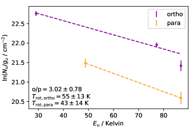
Figure 7: Disk-averaged rotational diagram of the unblended lines. We find similar ortho and para rotational temperatures and a disk integrated ortho-to-para ratio consistent with 3.

So where does this ortho-to-para ratio come from? Both ortho and para forms of $c-$C₃H₂ mainly form via gas phase reactions (e.g., Vrtilek et al., 1987; Park et al., 2006), in particular via C₃H⁺ reacting with H₂ via radiative association. Morisawa et al. (2006) demonstrate that the ortho-to-para ratio of $c-$C₃H₂ in steady state can be approximated by:

$$[o/p]_{\rm C_{3}H_{2}}=\frac{(5+3\phi)\times[o/p]_{\rm H_{2}}+3\phi+3}{(1+\phi)\times[o/p]_{\rm H_{2}}+\phi+3},$$ (1)

where $\phi$ essentially reflects the ratio of the rate of formation of $c-$C₃H₂ by electron dissociative recombination of C₃H${}_{3}^{+}$ compared to reactions of C₃H${}_{3}^{+}$ with atoms (however, see also the discussion in Park et al., 2006, for additional effects). The parameter $\phi$ is equal to $k_{\rm DR}[n_{e}]/k_{\rm ion-Y}[n_{\rm Y}]$, where $k_{\rm DR}$ is the rate of dissociative recombination, $n_{e}$ is the number density of electrons, $k_{\rm ion-Y}$ is the reaction rate of C₃H${}_{3}^{+}$ with species Y and $[n_{\rm Y}]$ is the number density of said species. If the ortho-to-para ratio of H₂ goes to 3, the dependence on $\phi$ drops out of Equation 1. If the ortho-to-para ratio of H₂ is small due to a cold formation mechanism of H₂, then the ortho-to-para ratio of $c-$C₃H₂ depends on $\phi$, going to 1 if $\phi$ is small and 3 if $\phi$ is large. Therefore, if this equation holds, obtaining the observed ortho to para ratio of 3 in $c-$C₃H₂ means either H₂ has an ortho-to-para of 3, or $\phi$ is large.

We can estimate what $\phi$ regime $c-$C₃H₂ may be in using the Cleeves et al. (2018) model of a solar nebula like disk. Taking approximate values from a location of r = 50 au and $z/r$ of 0.3 au, the electron density is approximately $10^{-9}$ per H, and is largely governed by photoionization of atomic carbon. The recombination rate with electrons is approximately 10^-6 cm³ s^-1 at 50 K (Loison et al., 2017). For the denominator, if we take reactions with C as representative, the rate is $\sim 10^{-9}$ cm³ s^-1, and the abundance is also $10^{-9}$ per H. Therefore, $\phi$ comes down to the ratio of the rate coefficients, which is $>>1$. Therefore it is not clear whether our measured $c-$C₃H₂ ortho to para ratio is shedding light on the ortho-to-para ratio of H₂ or if it is related to the relative rate of dissociative recombination.

5.5 C/O implications for forming planets

While there are exciting prospects to use hydrocarbons to constrain C/O ratios in disks to connect with planets, we must understand what region our observations fundamentally probe. Our results find that the $c-$C₃H₂ emission largely comes from the UV irradiated layer, above an $A_{V}$ of 1 ($z/r>0.25$). While this implies we are not directly tracing the midplane regions where planets gain most of their gas mass, it is still informative in the quest to understand what compositions planets might accrete. The bright hydrocarbon emission has been attributed to high gas-phase C/O ratios, much greater than solar (Du et al., 2015; Kama et al., 2016; Bergin et al., 2016; Miotello et al., 2019). Either the molecular layer has a carbon enhancement (perhaps due to carbon grain destruction) or an oxygen deficit, or both. The simplest explanation for an oxygen deficit is the growth of water-ice rich grains leading to the formation of larger, midplane bound pebbles or even larger bodies as suggested by Hogerheijde et al. (2011) and consistent with models of Krijt et al. (2016). A midplane ice enrichment might facilitate enhanced planet formation via an increase in solid mass, and a larger reservoir of water ice from which planets could accrete, perhaps a good scenario for forming habitable planets.

Recently, in the HD 163296 disk, Teague et al. (2019) discovered a velocity pattern in CO gas emission consistent with in-fall from the surface toward annular disk gaps. These results imply the surface gas in the disk is feeding potential planet forming regions, and that with our observations we could be tracing the same gas reservoir that might feed proto-giant planets’ atmospheres (see also Cridland et al., 2020). Specifically in TW Hya, Teague et al. (2019) found evidence of vertical motion around 90 au, near the van Boekel et al. (2016) scattered light gap. If such motions are common, this would be exciting as the layer traced by $c-$C₃H₂ would be more directly related to the chemistry that sets planets’ atmospheric compositions.

Along these lines, the 20 Myr-old HR 8799 system’s four outer planets have been independently chemically characterized using VLT SPHERE, and their C/O ratios radially varies (Lavie et al., 2017; Bonnefoy et al., 2016). The inner two planets ($d$ at 24 au and $e$ at 15 au; Marois et al., 2008, 2010) have low C/O ratios – consistent with zero due to low C/H, while the outer two planets ($b$ at 38 au and $c$ at 68 au) have far larger C/O ratios of 0.8 – 0.9 (Lavie et al., 2017). More recently, Mollière et al. (2020) reevaluated the atmospheric C/O ratios for planet $e$ and found a C/O value of 0.6, so less extreme of a jump than previously estimated. These results emphasize the need for careful treatment of non-equilibrium atmospheric effects and care in interpreting individual C/O estimates.

Interestingly, HR 8799’s tentative radial increase from sub-solar/solar up to super solar values in C/O is spatially consistent with TW Hya’s increase in hydrocarbon emission. In fact, the radial separation of the inner planets falls interior to the start of TW Hya’s hydrocarbon ring, while the outer planets’ orbits are within the radial bounds of the hydrocarbon ring. Of course there are many differences between TW Hya and the HR 8799 system, including that HR 8799’s host star has a mass of 1.5 M_⊙ compared to TW Hya’s 0.8 M_⊙, so such a connection is purely speculative. However, an interesting feature worth pointing out is that the younger disk IM Lup does not show the same large inner ring in hydrocarbons (Cleeves et al., 2018), and instead has a more centrally peaked/flattened distribution. Rings do appear to be common among intermediate aged disks (Bergin et al., 2016; Bergner et al., 2019), including some of the $\gtrsim 1$ Myr disks in Lupus (Miotello et al., 2019). For example the 3-10 Myr (Bertout et al., 2007) DM Tau disk also shows a combination of an inner hydrocarbon enhancement and a secondary outer ring (Bergin et al., 2016). If this qualitative observation is a truly common feature, perhaps the varied atmospheric C/O in HR 8799’s planets indicate the system formed “chemically later” in a disk more like TW Hya than early like IM Lup. Additional observations of hydrocarbon morphologues coupled with modeling that brings together chemistry and gas-giant formation simulations are necessary to fully test this hypothesis.

Example central channels (velocity averaged for clarity) of the observed $c-$C₃H₂ transitions toward TW Hya and the masks used to clean the data and generate the moment-0 maps.

References

- Aikawa et al. (2002) Aikawa, Y., van Zadelhoff, G. J., van Dishoeck, E. F., & Herbst, E. 2002, A&A, 386, 622
- Anderson et al. (2017) Anderson, D. E., Bergin, E. A., Blake, G. A., et al. 2017, ApJ, 845, 13
- Andrews et al. (2012) Andrews, S. M., Wilner, D. J., Hughes, A. M., et al. 2012, ApJ, 744, 162
- Andrews et al. (2016) Andrews, S. M., Wilner, D. J., Zhu, Z., et al. 2016, ApJ, 820, L40
- Ansdell et al. (2016) Ansdell, M., Williams, J. P., van der Marel, N., et al. 2016, ApJ, 828, 46
- Bergin et al. (2014) Bergin, E. A., Cleeves, L. I., Crockett, N., & Blake, G. A. 2014, Faraday Discussions, 168, 61
- Bergin et al. (2016) Bergin, E. A., Du, F., Cleeves, L. I., et al. 2016, ArXiv e-prints, arXiv:1609.06337
- Bergin et al. (2010) Bergin, E. A., Hogerheijde, M. R., Brinch, C., et al. 2010, A&A, 521, L33+
- Bergin et al. (2013) Bergin, E. A., Cleeves, L. I., Gorti, U., et al. 2013, Nature, 493, 644
- Bergner et al. (2019) Bergner, J. B., Öberg, K. I., Bergin, E. A., et al. 2019, ApJ, 876, 25
- Bertout et al. (2007) Bertout, C., Siess, L., & Cabrit, S. 2007, A&A, 473, L21
- Bonnefoy et al. (2016) Bonnefoy, M., Zurlo, A., Baudino, J. L., et al. 2016, A&A, 587, A58
- Bosman et al. (2021) Bosman, A. D., Alarcon, F., Zhang, K., & Bergin, E. A. 2021, arXiv e-prints, arXiv:2101.12502
- Calahan et al. (2020) Calahan, J., Bergin, E. A., & al, e. 2020, ApJ, 0
- Cazzoletti et al. (2018) Cazzoletti, P., van Dishoeck, E. F., Visser, R., Facchini, S., & Bruderer, S. 2018, A&A, 609, A93
- Chandra & Kegel (2000) Chandra, & Kegel. 2000, Astron. Astrophys. Suppl. Ser., 142, 113. https://doi.org/10.1051/aas:2000142
- Cleeves et al. (2014) Cleeves, L. I., Bergin, E. A., Alexander, C. M. O. ., et al. 2014, Science, 345, 1590
- Cleeves et al. (2015) Cleeves, L. I., Bergin, E. A., Qi, C., Adams, F. C., & Öberg, K. I. 2015, ApJ, 799, 204
- Cleeves et al. (2018) Cleeves, L. I., Öberg, K. I., Wilner, D. J., et al. 2018, ApJ, 865, 155
- Cridland et al. (2020) Cridland, A. J., Bosman, A. D., & van Dishoeck, E. F. 2020, A&A, 635, A68
- Cuadrado et al. (2015) Cuadrado, S., Goicoechea, J. R., Pilleri, P., et al. 2015, A&A, 575, A82
- Debes et al. (2013) Debes, J. H., Jang-Condell, H., Weinberger, A. J., Roberge, A., & Schneider, G. 2013, ApJ, 771, 45
- Drozdovskaya et al. (2019) Drozdovskaya, M. N., van Dishoeck, E. F., Rubin, M., Jørgensen, J. K., & Altwegg, K. 2019, MNRAS, 490, 50
- Du et al. (2015) Du, F., Bergin, E. A., & Hogerheijde, M. R. 2015, ApJ, 807, L32
- Du et al. (2017) Du, F., Bergin, E. A., Hogerheijde, M., et al. 2017, ApJ, 842, 98
- Eistrup et al. (2018) Eistrup, C., Walsh, C., & van Dishoeck, E. F. 2018, A&A, 613, A14
- Favre et al. (2015) Favre, C., Bergin, E. A., Cleeves, L. I., et al. 2015, ArXiv e-prints, arXiv:1503.02659
- Favre et al. (2013) Favre, C., Cleeves, L. I., Bergin, E. A., Qi, C., & Blake, G. A. 2013, ApJ, 776, L38
- Fedele & Favre (2020) Fedele, D., & Favre, C. 2020, arXiv e-prints, arXiv:2005.03891
- Gaia Collaboration et al. (2016) Gaia Collaboration, Brown, A. G. A., Vallenari, A., et al. 2016, ArXiv e-prints, arXiv:1609.04172
- Guilloteau et al. (2016) Guilloteau, S., Reboussin, L., Dutrey, A., et al. 2016, A&A, 592, A124
- Hogerheijde & van der Tak (2000) Hogerheijde, M. R., & van der Tak, F. F. S. 2000, A&A, 362, 697
- Hogerheijde et al. (2011) Hogerheijde, M. R., Bergin, E. A., Brinch, C., et al. 2011, Science, 334, 338
- Huang et al. (2018) Huang, J., Andrews, S. M., Cleeves, L. I., et al. 2018, ApJ, 852, 122
- jpegues (2020) jpegues. 2020, jpegues/kepmask: Python Package: pykepmask v2.0.0, vv2.0.0, Zenodo, doi:10.5281/zenodo.3672187. https://doi.org/10.5281/zenodo.3672187
- Kama et al. (2016) Kama, M., Bruderer, S., van Dishoeck, E. F., et al. 2016, A&A, 592, A83
- Kastner et al. (2014) Kastner, J. H., Hily-Blant, P., Rodriguez, D. R., Punzi, K., & Forveille, T. 2014, ApJ, 793, 55
- Kastner et al. (2015) Kastner, J. H., Qi, C., Gorti, U., et al. 2015, ApJ, 806, 75
- Kreidberg et al. (2015) Kreidberg, L., Line, M. R., Bean, J. L., et al. 2015, ApJ, 814, 66
- Krijt et al. (2016) Krijt, S., Ciesla, F. J., & Bergin, E. A. 2016, ApJ, 833, 285
- Krijt et al. (2018) Krijt, S., Schwarz, K. R., Bergin, E. A., & Ciesla, F. J. 2018, ApJ, 864, 78
- Lacour et al. (2019) Lacour, S., Nowak, M., Wang, J., et al. 2019, VizieR Online Data Catalog, J/A+A/623/L11
- Lavie et al. (2017) Lavie, B., Mendonça, J. M., Mordasini, C., et al. 2017, AJ, 154, 91
- Loison et al. (2017) Loison, J.-C., Agúndez, M., Wakelam, V., et al. 2017, MNRAS, 470, 4075
- Loomis et al. (2018) Loomis, R. A., Cleeves, L. I., Öberg, K. I., et al. 2018, ApJ, 859, 131
- Madhusudhan (2012) Madhusudhan, N. 2012, ApJ, 758, 36
- Madhusudhan et al. (2011) Madhusudhan, N., Harrington, J., Stevenson, K. B., et al. 2011, Nature, 469, 64
- Marois et al. (2008) Marois, C., Macintosh, B., Barman, T., et al. 2008, Science, 322, 1348
- Marois et al. (2010) Marois, C., Zuckerman, B., Konopacky, Q. M., Macintosh, B., & Barman, T. 2010, Nature, 468, 1080
- Miotello et al. (2019) Miotello, A., Facchini, S., van Dishoeck, E. F., et al. 2019, A&A, 631, A69
- Mollière et al. (2020) Mollière, P., Stolker, T., Lacour, S., et al. 2020, A&A, 640, A131
- Morisawa et al. (2006) Morisawa, Y., Fushitani, M., Kato, Y., et al. 2006, ApJ, 642, 954
- Müller et al. (2005) Müller, H. S. P., Schlöder, F., Stutzki, J., & Winnewisser, G. 2005, Journal of Molecular Structure, 742, 215
- Öberg & Bergin (2016) Öberg, K. I., & Bergin, E. A. 2016, ApJ, 831, L19
- Öberg et al. (2011) Öberg, K. I., Murray-Clay, R., & Bergin, E. A. 2011, ApJ, 743, L16
- Öberg et al. (2017) Öberg, K. I., Guzmán, V. V., Merchantz, C. J., et al. 2017, ApJ, 839, 43
- Park et al. (2006) Park, I. H., Wakelam, V., & Herbst, E. 2006, A&A, 449, 631
- Pegues et al. (2020) Pegues, J., Öberg, K. I., Bergner, J. B., et al. 2020, ApJ, 890, 142
- Qi et al. (2013a) Qi, C., Öberg, K. I., Wilner, D. J., & Rosenfeld, K. A. 2013a, ApJ, 765, L14
- Qi et al. (2008) Qi, C., Wilner, D. J., Aikawa, Y., Blake, G. A., & Hogerheijde, M. R. 2008, ApJ, 681, 1396
- Qi et al. (2006) Qi, C., Wilner, D. J., Calvet, N., et al. 2006, ApJ, 636, L157
- Qi et al. (2013b) Qi, C., Öberg, K. I., Wilner, D. J., et al. 2013b, Science, 341, 630
- Salinas et al. (2016) Salinas, V. N., Hogerheijde, M. R., Bergin, E. A., et al. 2016, A&A, 591, A122
- Schöier et al. (2005) Schöier, F. L., van der Tak, F. F. S., van Dishoeck, E. F., & Black, J. H. 2005, A&A, 432, 369
- Schwarz et al. (2016) Schwarz, K. R., Bergin, E. A., Cleeves, L. I., et al. 2016, ApJ, 823, 91
- Teague (2019) Teague, R. 2019, The Journal of Open Source Software, 4, 1632
- Teague et al. (2019) Teague, R., Bae, J., & Bergin, E. A. 2019, Nature, 574, 378
- Teague et al. (2018) Teague, R., Henning, T., Guilloteau, S., et al. 2018, ApJ, 864, 133
- Trapman et al. (2019) Trapman, L., Facchini, S., Hogerheijde, M. R., van Dishoeck, E. F., & Bruderer, S. 2019, A&A, 629, A79
- van Boekel et al. (2016) van Boekel, R., Henning, T., Menu, J., et al. 2016, ArXiv e-prints, arXiv:1610.08939
- Visser et al. (2011) Visser, R., Doty, S. D., & van Dishoeck, E. F. 2011, A&A, 534, A132
- Visser et al. (2009) Visser, R., van Dishoeck, E. F., Doty, S. D., & Dullemond, C. P. 2009, A&A, 495, 881
- Vrtilek et al. (1987) Vrtilek, J. M., Gottlieb, C. A., & Thaddeus, P. 1987, ApJ, 314, 716
- Walsh et al. (2014) Walsh, C., Millar, T. J., Nomura, H., et al. 2014, A&A, 563, A33
- Weinberger et al. (2002) Weinberger, A. J., Becklin, E. E., Schneider, G., et al. 2002, ApJ, 566, 409
- Yu et al. (2017) Yu, M., Evans, Neal J., I., Dodson-Robinson, S. E., Willacy, K., & Turner, N. J. 2017, ApJ, 850, 169
- Zhang et al. (2017) Zhang, K., Bergin, E. A., Blake, G. A., Cleeves, L. I., & Schwarz, K. R. 2017, Nature Astronomy, 1, 0130