Knowledge Hypergraph Embedding Meets Relational Algebra

Abstract

Embedding-based methods for reasoning in knowledge hypergraphs learn a representation for each entity and relation. Current methods do not capture the procedural rules underlying the relations in the graph. We propose a simple embedding-based model called ReAlE that performs link prediction in knowledge hypergraphs (generalized knowledge graphs) and can represent high-level abstractions in terms of relational algebra operations. We show theoretically that ReAlE is fully expressive and provide proofs and empirical evidence that it can represent a large subset of the primitive relational algebra operations, namely renaming, projection, set union, selection, and set difference. We also verify experimentally that ReAlE outperforms state-of-the-art models in knowledge hypergraph completion, and in representing each of these primitive relational algebra operations. For the latter experiment, we generate a synthetic knowledge hypergraph, for which we design an algorithm based on the Erdős-Rényi model for generating random graphs.

1 Introduction

Knowledge hypergraphs are knowledge bases that store information about the world in the form of tuples describing relations among entities. They can be seen as a generalization of knowledge graphs in which relations are defined on two entities. In recent times, the most dominant paradigm has been to learn and reason on knowledge graphs. However, hypergraphs are the original structure of many existing graph datasets. Wen et al. (2016) observe that in the original Freebase (Bollacker et al., 2008) more than $1/3$rd of the entities participate in non-binary relations (i.e., defined on more than two entities). Fatemi et al. (2020) observe, in addition, that $61$% of the relations in the original Freebase are non-binary. Similar to knowledge graphs, knowledge hypergraphs are incomplete because curating and storing all the true information in the world is difficult. The goal of link prediction in knowledge hypergraphs (or knowledge hypergraph completion) is to predict unknown links or relationships among entities based on existing ones. While it is possible to convert a knowledge hypergraph into a knowledge graph and apply existing methods on it, Wen et al. (2016) and Fatemi et al. (2020) show that embedding-based methods for knowledge graph completion do not work well out of the box for knowledge graphs obtained through such conversion techniques.

Most of the models developed to perform link prediction in knowledge hypergraphs are extensions of those used for link prediction in knowledge graphs. But a model designed to reason over binary relations does not necessarily generalize well to non-binary relations. Furthermore, it is not clear if the existing models for knowledge hypergraph completion effectively capture the relational semantics underlying the knowledge hypergraphs. Recent research (Battaglia et al., 2018; Teru et al., 2020) has highlighted the role of relational inductive biases in building learning agents that learn entity-independent relational semantics and reason in a compositional manner. Such agents can generalize better to unseen structures. In this work, we are interested in exploring the foundations of the knowledge hypergraph completion task; we thus aim to design a model for reasoning in knowledge hypergraphs that is simple, expressive, and can represent high-level abstractions in terms of relational algebra operations. We hypothesize that models that can reason about relations in terms of relational algebra operations have better generalization power.

Relational algebra is a formalization that is at the core of relational models (e.g., relational databases). It consists of several primitive operations that can be combined to synthesize all other operations used. Each such operation takes relations as input and returns a relation as output. In a knowledge hypergraph, these operations can describe how relations depend on each other. To illustrate the connection between relational algebra operations and relations in knowledge hypergraphs, consider the example in Figure 1 that shows samples from some knowledge hypergraph. The relations in the example feature the two primitive relational algebra operations renaming and projection. Relation $bought$ is a renaming of $sold$. Relation $buyer$ is a projection of relation $sold$. If a model is able to represent these two operations, it can potentially learn that a tuple $bought(X,Y,I)$ (person $X$ bought from person $Y$ item $I$) is implied by tuple $sold(Y,X,I)$ (person $Y$ sold to person $X$ item $I$); or that a tuple $buyer(X,I)$ (person $X$ is the buyer of item $I$) is implied by the tuple $sold(Y,X,I)$. An embedding model that cannot represent the relational algebra operations renaming and projection would not be able to learn that relation $bought$ in Figure 1 is a renaming of relation $sold$. It would thus be difficult for such a model to reason about the relationship between these two relations. In contrast, a model that can represent renaming and projection operations is potentially able to determine that $bought(alex,drew,book)$ is true because the train set contains $sold(drew,alex,book)$ and $bought$ is a renaming of $sold$.

Designing reasoning methods that can capture the relational semantics in terms of relational algebra is especially important in the context of knowledge hypergraphs, where many relations are defined on more than two entities. Domains with beyond-binary relations often provide multiple methods of expressing the same underlying notion, as seen in the above example where relations $sold$ and $bought$ encode the same information. In contrast, since all relations in a knowledge graph are binary (have arity $2$), many of the relational algebra operations (such as projection, which changes the arity of the relation) are not applicable to this setting. This also highlights the importance of knowledge hypergraphs as a data model that encodes rich relational structures ripe for further exploration.

Figure 1: An example of a knowledge hypergraph split into train and test sets. The train set contains tuples $sold(drew,alex,book)$, $buyer(alex,book)$, $sold(mike,sam,tv)$, and $bought(sam,mike,tv)$. Relation $bought$ can be obtained by applying a renaming operation to relation $sold$. Similarly, relation $buyer$ is a projection of relation $sold$. Learning these relational algebra operations can help the model generalize better to the tuples in the test set. The test responses, from top to bottom, are $drew$, $tv$, and $mike$.

Our goal in this work is to design a knowledge hypergraph model that is simple, expressive, and can provably represent relational algebra operations. To achieve this, we propose a model called ReAlE. We show theoretically that ReAlE can represent the operations renaming, projection, selection, set union, and set difference, and experimentally verify that it performs well in predicting such relations in existing knowledge bases. We further prove that ReAlE is fully expressive. The contributions of this work are as follows.

1. ReAlE, an embedding-based method for knowledge hypergraph completion that can provably represent the relational algebra operations renaming, projection, set union, selection, and set difference,

2. experimental results that show that ReAlE outperforms the state-of-the-art on well-known public datasets, and

3. a framework for generating synthetic knowledge hypergraphs, which is based on the Erdős-Rényi random graph generation model and can generate relations by repeated application of primitive relational algebra operations. Such datasets can serve as benchmarks for evaluating the relational algebraic generalization power of knowledge hypergraph completion methods. We use our algorithm to generate the dataset REL-ER (RELational Erdős-Rényi) and use it in our experiments.

2 Related Work

Existing work in the area of knowledge hypergraph completion can be grouped into the following categories.

Statistical Relational Learning. Models under the umbrella of statistical relational learning (Raedt et al., 2016) can handle variable arity relations and explicitly model the interdependencies of relations. Our work is complementary to these approaches in that ReAlE is an embedding-based model that represents relational algebra operations implicitly, rather than representing them explicitly.

Translational approaches. Models in this category are extensions of translational approaches for binary relations to beyond-binary. One of the earliest models in this category is m-TransH (Wen et al., 2016), which extends TransH (Wang et al., 2014) to knowledge hypergraph embedding. RAE (Zhang et al., 2018) extends m-TransH by adding the relatedness of values – the likelihood that two values co-participate in a common instance – to the loss function. NaLP (Guan et al., 2019) uses a similar strategy to RAE, but models the relatedness of values based on the roles they play in different tuples. Models in this category have severe restrictions on the types of relations they can model. Liu et al. (2020) discuss these limitations, and we address them more formally in Section 5.

Tensor factorization based approaches. Models in this category extend tensor factorization models for knowledge graph completion to knowledge hypergraph completion. Liu et al. (2020) propose GETD, which extends Tucker (Balažević et al., 2019) to n-ary relations. GETD is fully expressive. However, given that for each relation it learns a tensor with a dimension equal to the arity of the relation, the memory and time complexity of GETD grow exponentially with the arity of relations in the dataset. Fatemi et al. (2020) propose HypE which is motivated by SimplE (Kazemi & Poole, 2018). HypE disentangles the embeddings of relations from the positions of its arguments and thus the memory and time complexity grows linearly with the arity of the relations in the dataset. HypE is fully expressive but cannot represent some relational algebra operations. We discuss this in Section 5.

Key-value pair based approaches. Models in this category, such as NeuInfer and HINGE (Guan et al., 2020; Rosso et al., 2020), assume that a tuple is composed of a triple (binary relation), plus a list of attributes in the form of key-value pairs. The problem these works study is slightly different as we consider all information as part of a tuple. They evaluate their models on datasets for which they obtain the tuple attributes from external data sources using heuristics and thus their results are not comparable to ours.

Graph neural networks approaches. These approaches extend graph neural networks to hypergraph neural networks (Feng et al., 2019; Yadati et al., 2018). G-MPNN (Yadati, 2020) further extends these models to knowledge hypergraphs (directed and labeled hyperedges). The G-MPNN scoring function assumes relations are symmetric, and thus has restrictions in modeling the non-symmetric relations and is not fully expressive.

Present work. Reasoning in hypergraphs is a relatively underexplored area that has recently gained more attention. While the methods above show promise, none of them offer more understanding of the knowledge hypergraph completion task, as these works lack theoretical analysis of the models they propose and do not provide evidence to the type of entity-independent relational semantic they can model. In this work, we design a model based on relational algebra which is the calculus of relational models. Besides the theoretical contributions, we show empirically how basing our model on relational algebra operations give us improvements compared to the existing works.

3 Definition and Notation

Assume a finite set of entities ${\mathcal{E}}$ and a finite set of relations ${\mathcal{R}}$. Each relation has a fixed non-negative integral arity. A tuple is the form of $r(x_{1},\dots,x_{n})$ where $r\in{\mathcal{R}}$, $n=|r|$ is the arity of $r$, and each $x_{i}\in{\mathcal{E}}$. Let $\tau$ be the set of ground truth tuples; it specifies all of the tuples that are true. If a tuple is not in $\tau$, it is false. A knowledge hypergraph consists of a subset of the tuples $\tau^{\prime}\subseteq\tau$. Knowledge hypergraph completion is the problem of predicting the missing tuples in $\tau^{\prime}$, that is, finding the tuples $\tau\setminus\tau^{\prime}$. A knowledge graph is a special case of a knowledge hypergraph where all relations have arity $2$.

An embedding is a function from an entity or a relation to a vector or a matrix (or a higher-order tensor) over a field. We use bold lower-case for embeddings, that is, $\mathbf{x}$ is the embedding of entity $x$, and $\mathbf{r}$ is the embedding of relation $r$. For the task of knowledge hypergraph completion, an embedding-based model having parameters $\theta$ defines a function $\phi_{\theta}$ that takes a tuple as input and generates a prediction, e.g., a probability (or a score) of the tuple being true. A model is fully expressive if given any assignment of truth values to all tuples, there exists an assignment of values to $\theta$ that accurately separates the true tuples from the false ones.

Following Python notation, $\mathbf{x}[k]$ is the $k$-th index of vector $\mathbf{x}$ and $\mathbf{r}[i][k]$ is the $i$-th row and $k$-th column of matrix $r$. We use $\times$ for multiplication of two scalars. The bijective function $\pi:\{1,\dots,n\}\rightarrow\{1,\dots,n\}$ takes a sequence $(x_{1},x_{2},\dots,x_{n})$ and outputs a sequence $(x_{\pi(1)},x_{\pi(2)},\dots,{x_{\pi(n)}})$. For example, if $\pi=\{1\mapsto 2,2\mapsto 1,3\mapsto 3\}$ then, $(x_{\pi(1)},x_{\pi(2)},x_{\pi(3)})=(x_{2},x_{1},x_{3})$.

4 Proposed Method

ReAlE (Relational Algebra Embedding) is a knowledge hypergraph completion model that has parameters $\theta$ and a scoring function ${\phi_{\theta}}$. We motivate our model bottom-up by first describing an intuitive model for this task (Equation 1); we then discuss why this formulation would not work well and adjust it in ReAlE (Equation 10).

Given a tuple $r(x_{1},\dots,x_{n})$, determining whether it is true or false depends on the relation and the entities involved; it also depends on the position of each entity in the tuple, as the role of an entity changes with its position and relation. For example, the role of $drew$ is different in the tuples $sold(drew,alex,book)$ and $sold(alex,drew,book)$ as the position of $drew$ is different. The role of $drew$ is also different in the tuples $sold(drew,alex,book)$ and $bought(drew,alex,book)$ as the relation is different.

An intuitive model to decide whether a tuple is true or not is one that embeds each entity $x_{i}\in{\mathcal{E}}$ into a vector $\mathbf{x_{i}}\in[0,1]^{d}$ of length $d$, and the relation $r$ into a matrix $\mathbf{r}\in\mathbb{R}^{|r|\times d}$, where the $i^{th}$ row in $\mathbf{r}$ operates over the entity at position $i$. Each relation $r$ has a bias term $b_{r}$ as a relation dependent constant that does not depend on any entities and allows the model to have the flexibility to search through the solution space (similar to a bias term in linear regression). Such a model defines a score for a tuple. This score may be interpreted as “the higher the score, the more likely it is that the tuple is true”, and can be expressed as follows:

$${\phi^{\circ}_{\theta}}{} (r(x_{1},\dots,x_{n}))=\sigma\left(b_{r}+\sum_{i=1}^{|r|}\sum_{k=0}^{d-1}\mathbf{x_{i}}[k]\times\mathbf{r}[i][k]\right)$$ (1)

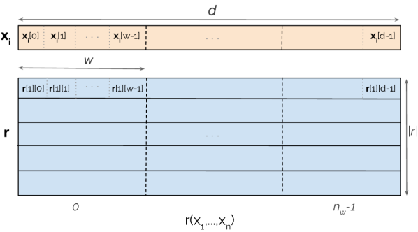
Figure 2: A schematic of the entity and relation embeddings in ReAlE: the embedding dimension $d$ is divided into $n_{w}$ windows of size $w$.

The above scoring function is similar to Canonical Polyadic (Hitchcock, 1927) for tensor decomposition, as the same indices in the embedding of entities and relations are multiplied and the final score is the result of summing these multiplications. Studies (Kazemi & Poole, 2018; Lacroix et al., 2018), however, show that designs similar to that in Equation 1 do not properly model the interaction between embeddings of entities and relations at different indices, and that by adding interaction among different elements of the embeddings in different indices, the information flows better and the performance improves.

Therefore, one missing component in Equation 1 is the interaction of different elements of the embeddings. To create such an interaction, we introduce the concept of windows, a range of indices whereby elements within the same window interact with each other. ReAlE uses windows to increase interaction between embeddings; it then uses a nonlinear function $\sigma$ to obtain the contribution of each window, which are then added to produce a score. The number of embedding elements for each entity in a window is the window size and is a hyperparameter (see Figure 2). Let $w$ denote the window size, $n_{w}=\lfloor\frac{d}{w}\rfloor$ the number of windows, and $b_{r}^{j}$ the bias term of relation $r$ for the $j^{th}$ window, for all $j=0,\dots,n_{w}-1$. Equation 10 defines ReAlE’s score of a tuple $r(x_{1},x_{2},\dots,x_{n})$, where $\sigma$ is a monotonically-increasing nonlinear function that is differentiable almost everywhere.

$$\begin{split}&{\phi_{\theta}}(r(x_{1},\dots,x_{n}))=\\ &\frac{1}{n_{w}}\sum_{j=0}^{n_{w}-1}\sigma\left(b_{r}^{j}+\sum_{i=1}^{|r|}\sum_{k=0}^{w-1}\mathbf{x_{i}}[jw+k]\times\mathbf{r}[i][jw+k]\right)\end{split}$$ (2)

Learning ReAlE Model.

To learn a ReAlE model, we use stochastic gradient descent with mini-batches. In each learning iteration, we take in a batch of positive tuples from the knowledge hypergraph. As a knowledge hypergraph typically only has positive instances and we need to also train our model on negative instances, we generate negative examples by following the contrastive approach of Bordes et al. (2013).

Given a knowledge hypergraph defined on $\tau^{\prime}$, we let $\tau^{\prime}_{\mathrm{train}}$, $\tau^{\prime}_{\mathrm{test}}$, and $\tau^{\prime}_{\mathrm{valid}}$ denote the (pairwise disjoint) train, test, and validation sets, respectively, so that $\tau^{\prime}=\tau^{\prime}_{\mathrm{train}}\sqcup\tau^{\prime}_{\mathrm{test}}\sqcup\tau^{\prime}_{\mathrm{valid}}$ where $\sqcup$ is disjoint set union. To build a model that completes $\tau^{\prime}$, we train it using $\tau^{\prime}_{\mathrm{train}}$, tune the hyperparameters of the model using $\tau^{\prime}_{\mathrm{valid}}$, and evaluate its efficacy on $\tau^{\prime}_{\mathrm{test}}$. For any tuple $t$ in $\tau^{\prime}$, we let $T_{\mathrm{neg}}(t)$ be a function that generate a set of related negative samples. We define the following cross entropy loss that has been shown to be effective for link prediction (Kadlec et al., 2017).

$$\mathcal{L}(\theta,\tau^{\prime}_{\mathrm{batch}})=\sum_{t\in\tau^{\prime}_{\mathrm{batch}}}{-\log\left(\frac{\mathrm{e}^{{\phi_{\theta}}(t)}}{\displaystyle\sum_{t^{\prime}\in~{}\{t\}~{}\cup~{}T_{\mathrm{neg}}(t)}{\mathrm{e}^{{\phi_{\theta}}(t^{\prime})}}}\right)}$$ (3)

Here, $\theta$ represents parameters of the model including relation and entity embeddings, and ${\phi_{\theta}}$ is the function given by Equation (10) that maps a tuple to a score using parameters $\theta$, and $\tau^{\prime}_{batch}$ is a batch of tuples in $\tau^{\prime}_{train}$. Algorithm 1 shows a high-level description of how we train a ReAlE model.

Algorithm 1 Learning ReAlE

Input: Tuples $\tau^{\prime}_{train}$, loss function $\mathcal{L}$, scoring function ${\phi_{\theta}}{}$

Output: Embeddings $\mathbf{x}$ and $\mathbf{r}$ for all entities and relations in $\tau^{\prime}_{train}$.

Initialize $\mathbf{x}$ and $\mathbf{r}$ (at random)

for every batch $\tau^{\prime}_{\mathrm{batch}}$ of tuples in $\tau^{\prime}_{train}$ do

       for tuple $t$ in $\tau^{\prime}_{\mathrm{batch}}$ do

             Generate negative tuples $T_{neg}(t)$   for $t^{\prime}\in\{t\}\cup T_{neg}(t)$ do

                   Compute ${\phi_{\theta}}(t^{\prime})$      (Eq. 10) 

             end for

            

       end for

      Compute the loss $\mathcal{L}(\theta,\tau^{\prime}_{\mathrm{batch}})$              (Eq. 3)  Compute the gradient of loss with respect to $\mathbf{x}$ and $\mathbf{r}$   Update embeddings $\mathbf{x}$ and $\mathbf{r}$ through back-propagation  

end for

5 Theoretical Analysis

To better understand the expressive power of ReAlE and the types of reasoning it can perform, in this section we analyze the extent of its expressivity and its capacity to represent relational algebra operations without the operations being known or given to the learner.

Relational algebra allows for quantification, in particular for statements that are true for all entities or are true for at least one. To allow for such statements, we introduce the notion of variables, which, following the convention of Datalog, we write in upper case, e.g., $X_{1},\dots,X_{n}$. We use lower case $x_{1},\dots,x_{n}$ to denote particular entities. To make a meaningful statement, each variable is quantified using $\forall$ (the statement is true for all assignments of entities to the variable) and $\exists$ (the statement is true if there exists an assignment of an entity to the variable). $\bar{x}$ is a sequence of particular entities and $\bar{X}$ is a sequence of variables. The symbol $\neg$ is the negation operator.

For any $\bar{x}$ and any relation $r$, we define the relation complement function $f$ as $f({\phi_{\theta}}(r({\bar{x}})))={\phi_{\theta}}(\neg r({\bar{x}}))$. This function depends on the choice of the nonlinearity $\sigma$ of the scoring function in Equation 10. For example, if $\sigma$ is the Sigmoid function, then $f({\phi_{\theta}}(r({\bar{x}})))=1-{\phi_{\theta}}(r({\bar{x})})$; if it is the hyperbolic tangent (tanh), then $f({\phi_{\theta}}(r({\bar{x}})))=-{\phi_{\theta}}(r({\bar{x}}))$. In what follows, we assume that $f$ exists for the selected $\sigma$.

We defer all proofs to Appendix A.

5.1 Full Expressivity

The two results in this section state that ReAlE is fully expressive and that some other models are not.

Theorem 1 (Expressivity)

For any ground truth over entities $\mathcal{E}$ and relations $\mathcal{R}$ containing $\lambda$ true tuples with $\alpha=\max_{r\in{\mathcal{R}}}(|r|)$ as the maximum arity over all relations in $\mathcal{R}$, there is a ReAlE model with $n_{w}=\lambda$, $w=\alpha$, $d=\max(\alpha\lambda,\alpha)$, and $\sigma(x)=\frac{1}{1+\exp(-x)}$ that accurately separates the true tuples from the false ones.

Theorem 2

m-TransH, RAE, and NaLP are not fully expressive and have restrictions on the relations they can represent.

5.2 Representing Relational Algebra with ReAlE

In this section, we describe the primitive relational algebra operations and prove how closely ReAlE can represent each.

5.2.1 Renaming

Renaming changes the name of one or more entities in a relation. A renaming operation can be written as the following logical rule, where $t$ is defined in terms of $s$.

$$\forall X_{1},\dots,X_{n}~{}~{}~{}~{}~{}~{}~{}~{}t({X_{1},\dots,X_{n}})\leftrightarrow s(X_{\pi(1)},\dots,X_{\pi(n)})$$ (4)

For example, $\forall~{}X,Y,I~{}~{}bought(X,Y,I)\leftrightarrow~{}sold(Y,X,I)$ represents renaming relation (person X bought item I from person Y) into relation (person Y sold item I to person X).

Theorem 3 (Renaming)

Given permutation function $\pi$, and relation $s$, there exists a parametrization for relation $t$ in ReAlE such that for entities $x_{1},\dots,x_{n}$, with arbitrary embeddings,

$${\phi_{\theta}}(t(x_{1},\dots,x_{n}))={\phi_{\theta}}(s(x_{\pi(1)},x_{\pi(2)},\dots,x_{\pi(n)}))$$

5.2.2 Projection

A projection operation that defines $t$ as a projection of $s$ can be written as the following (for $m<n$).

$$\forall X_{1},\dots,X_{m}~{}t(X_{1},\dots,X_{m})~{}\\ \leftrightarrow\exists{X_{m+1},\dots,X_{n}}~{}~{}~{}~{}s(X_{1},\dots,X_{m},\dots,X_{n})$$ (5)

Note that projection can be paired with renaming to allow for arbitrary subsets and ordering of arguments. For example,

$$\forall X,I~{}seller(X,I)\leftrightarrow\exists P~{}bought(P,X,I)$$

Theorem 4 (Projection)

For any relation $s$ on $n$ arguments there exists a parametrization for relation $t$ on $m<n$ arguments in ReAlE such that for any arbitrary sequence $x_{1},\dots,x_{n}$

$${\phi_{\theta}}(t(x_{1},\dots,x_{m}))\geq{\phi_{\theta}}(s(x_{1},\dots,x_{n}))$$

Inequality is the best we can hope for, because multiple tuples with relation $s$ might project to the same tuple with relation $t$. The score of the tuple with relation $t$ should thus be greater than or equal to the maximum score for $s$.

5.2.3 Selection

Selection returns the subset of tuples of a relation that satisfy a given condition. Here, we consider equality conditions whereby a selection operation reduces the number of arguments, and has two forms defining $t$ as a selection of $s$.

$$\forall X_{1},\dots,X_{n}~{}~{}~{}~{}~{}~{}~{}t(X_{1},\dots,X_{p-1},X_{p+1},\dots,X_{q},\dots,X_{n})\\ \leftrightarrow\exists X_{p}~{}~{}s(X_{1},\dots,X_{n})\land(X_{p}=X_{q})$$ (6)

$$\forall X_{1},\dots,X_{n}~{}~{}~{}~{}~{}~{}~{}~{}~{}~{}~{}t(X_{1},\dots,X_{p-1},X_{p+1},\dots,X_{n})\\ \leftrightarrow\exists X_{p}~{}~{}~{}s(X_{1},\dots,X_{n})\land(X_{p}=c)\textrm{~{}~{}~{}for fixed }c$$ (7)

For example,

$$\forall X,Y~{}sold\_coffee(X,Y)\leftrightarrow\exists I~{}sold(X,Y,I)\land(I=coffee)$$

in which $sold\_coffee(X,Y)$ is true if $X$ sold coffee to $Y$.

Observe that selecting tuples with the condition $X_{p}=X_{q}$ for arbitrary $p$ and $q$ is equivalent to first renaming the tuple so that $X_{p}$ is in position $n$ and $X_{q}$ is in position $n-1$; and then performing a selection with the condition $X_{n-1}=X_{n}$ or $X_{n}=c$. Thus, to simplify our proofs, we show the selection operation for the case when $X_{n-1}=X_{n}$ and $X_{n}=c$.

Theorem 5 (Selection 1)

For arbitrary relation $s$, there exists a parametrization for relation $t$ in ReAlE such that for arbitrary entities $x_{1},\dots,x_{n}$

$${\phi_{\theta}}(t(x_{1},\dots,x_{n-1}))={\phi_{\theta}}(s(x_{1},\dots,x_{n-1},x_{n-1}))\\$$

Theorem 6 (Selection 2)

For arbitrary relation $s$ and for a fixed constant $c$, there exists a parametrization for relation $t$ in ReAlE such that for arbitrary entities $x_{1},\dots,x_{n}$

$${\phi_{\theta}}(t(x_{1},\dots,x_{n-1}))={\phi_{\theta}}(s(x_{1},\dots,x_{n-1},c))$$

5.2.4 Set Union

Set union operates on relations of the same arity, and returns a new relation containing the tuples that appear in at least one of the relations. A set union operation can be written as the following logical rule with relation $t$ as the union of $s$ and $r$.

$$\forall\bar{X}~{}~{}~{}~{}~{}~{}~{}~{}t(\bar{X})\leftrightarrow s(\bar{X})\lor r(\bar{X})$$ (8)

For example,

$$\forall X_{1},X_{2},I~{}~{}~{}traded(X_{1},X_{2},I)\\ \leftrightarrow~{}sold(X_{1},X_{2},I)\lor bought(X_{1},X_{2},I)$$

For a ReAlE model to be able to represent the set union operation, first observe that any score for a tuple $t$ that represents the union of relations $r$ and $s$ depends on how dependent the two relations $r$ and $s$ are. For example, if $s$ is a subset of $r$, then the score of $t$ is equal to that of $r$. But since we do not know about such dependence relations in the data, then the best we can hope for is a bound that shows that the score of $t$ is at least as high as the maximum score of either $r$ or $s$, as the following lemma states.

Theorem 7 (Set Union)

For arbitrary relations $s$ and $r$ with the same arity, there exists a parametrization for relation $t$ in ReAlE such that for arbitrary entity set $\bar{x}$

$${\phi_{\theta}}(t(\bar{x}))\geq\max({\phi_{\theta}}(s(\bar{x})),{\phi_{\theta}}(r(\bar{x})))$$

5.2.5 Set Difference

Set difference operates on relations of the same arity, and returns a new relation containing the tuples from the left relation that do not appear in the right one. The set difference operation can be written as the following logical rule, where relation $t$ is set difference of $s$ and $r$.

$$\forall\bar{X}~{}~{}~{}~{}~{}~{}~{}~{}t(\bar{X})\leftarrow s(\bar{X})\land\neg r(\bar{X})$$ (9)

For example, relation $needs\_filter(X,Y)$ is true if $X$ bought coffee but did not buy coffee filter from $Y$.

$$\forall X,Y~{}~{}needs\_filter(X,Y)\leftarrow bought\_coffee(X,Y)\land\\ \neg bought\_filter(X,Y)$$

Similar to set union, the score of a set difference operator depends on how dependent the relations $r$ and $s$ are. For the same reasons, the best we can hope for in this case is to show that the score of $t$ is smaller than that of both $s$ and $\neg r$ (since $t(\bar{X})$ is true only when both $s(\bar{X})$ and $\neg r(\bar{X})$ are true, then the scores of the latter two must be higher). In the lemma that follows, $f$ is the relation complement function described in the introduction of Section 5.

Theorem 8 (Set Difference)

For arbitrary relations $r$ and $s$ with the same arity, if $f$ is a linear relation complement function and $f(\sigma(x))=\sigma(c*x)$ with $c$ as a constant, there exists a parametrization for relation $t$ in ReAlE such that for arbitrary entities $x_{1},\dots,x_{n}$

$${\phi_{\theta}}(t(\bar{x}))\leq\min({\phi_{\theta}}(s(\bar{x})),f({\phi_{\theta}}(r(\bar{x}))))$$

Table 1: Knowledge hypergraph completion results on JF17K, FB-auto and m-FB15K for baselines and the proposed method. Our method ReAlE outperforms the baselines on all datasets. The sign “-” indicates that the corresponding paper has not provided the results. GETD is trained on a significantly smaller embedding dimension compared to the baselines to fit into the memory. Refer to Appendix C for implementation details of baselines and the proposed model.

	JF17K				FB-auto				m-FB15K
Model	MRR	Hit@1	Hit@3	Hit@10	MRR	Hit@1	Hit@3	Hit@10	MRR	Hit@1	Hit@3	Hit@10
m-DistMult (Fatemi et al., 2020)	0.463	0.372	0.510	0.634	0.784	0.745	0.815	0.845	0.705	0.633	0.740	0.844
m-CP (Fatemi et al., 2020)	0.392	0.303	0.441	0.560	0.752	0.704	0.785	0.837	0.680	0.605	0.715	0.828
m-TransH (Wen et al., 2016)	0.444	0.370	0.475	0.581	0.728	0.727	0.728	0.728	0.623	0.531	0.669	0.809
RAE (Zhang et al., 2018)	0.310	0.219	0.334	0.504	-	-	-	-	-	-	-	-
NaLP (Guan et al., 2019)	0.366	0.290	0.391	0.516	-	-	-	-	-	-	-	-
GETD (Liu et al., 2020)	0.151	0.104	0.151	0.258	0.367	0.254	0.422	0.601	-	-	-	-
HSimplE (Fatemi et al., 2020)	0.472	0.378	0.520	0.645	0.798	0.766	0.821	0.855	0.730	0.664	0.763	0.859
HypE (Fatemi et al., 2020)	0.494	0.408	0.538	0.656	0.804	0.774	0.823	0.856	0.777	0.725	0.800	0.881
G-MPNN (Yadati, 2020)	0.501	0.425	0.537	0.660	-	-	-	-	0.779	0.732	0.805	0.894
ReAlE (Ours)	0.530	0.454	0.563	0.677	0.861	0.836	0.877	0.908	0.801	0.755	0.823	0.901

5.3 Representing Relational Algebra with HypE

So far, we have established the theoretical properties of the proposed model and we showed that m-TransH, RAE, and NaLP (and G-MPNN in Section 2) are not fully expressive. In Appendix A.4, we further prove that HypE cannot represent all relational algebra operations. In particular, we show that HypE cannot represent selection.

6 Experimental Setup

In this section, we explain the datasets that are used in the experiments. We further explain the evaluation metrics used to compare models. We defer the implementation details of our model and baselines to Appendix C.

6.1 Datasets

To evaluate ReAlE for knowledge hypergraph completion, we conduct experiments on two classes of datasets.

Real-world datasets. We use three real-world datasets for our experiments: JF17K is proposed by Wen et al. (2016), and FB-AUTO and M-FB15K are proposed by Fatemi et al. (2020). Refer to Appendix B for statistics of the datasets.

Synthetic dataset. To study and evaluate the generalization power of models in a controlled environment, we also generate a synthetic dataset to use in our experiments. This practice has become common in recent years, with the creation of several procedurally generated benchmarks to study the generalization power of models in different tasks. Examples of such datasets include CLEVR (Johnson et al., 2017) for images, TextWorld (Côté et al., 2018) for text data, and GraphLog (Sinha et al., 2020) for graph data. To create a benchmark for analyzing the relational algebraic generalization power of ReAlE for hypergraph completion, we consider the following criteria.

1. Completeness: The benchmarks must contain the desired relational algebra operations; in our case: renaming, projection, selection, set union, and set difference.

2. Diversity: The benchmark must contain a variety of relations that are the result of repeated application of relational algebra operations having varying depth.

3. Compositional generalization: The benchmark must contain relations that are the result of repeated application of operations of different types.

To synthesize a dataset that satisfies the above conditions, we extend the Erdős-Rényi model (Erdős & Rényi, 1959) for generating random graphs to directed edge-labeled hypergraphs. We use this hypergraph generation model to first generate a given number of true tuples; we then apply the five relational algebra operations to these tuples (repeatedly and recursively) to obtain new tuples with varying depth. A detailed description of our extension to the Erdős-Rényi model and the full algorithm for generating the synthetic dataset can be found in Appendix B.

Table 2: Breakdown performance of MRR across composite relations (based on a sequence of primitive operations) and of varying depth on the REL-ER dataset along with their statistics.

		Operation type					Depth
Model	All	elementary	renaming	project	set union	set difference	1	2	3	4
m-TransH (Wen et al., 2016)	0.387	0.166	0.447	0.652	0.459	0.464	0.531	0.499	0.352	0.03
HypE (Fatemi et al., 2020)	0.689	0.335	0.877	0.856	0.888	0.894	0.881	0.872	0.897	0.976
ReAlE (Ours)	0.709	0.336	0.882	0.877	0.932	0.923	0.887	0.950	0.945	0.938
#tuples	5378	1833	458	762	1676	649	2075	1204	245	21

6.2 Evaluation Metrics

We evaluate the link prediction performance with two standard metrics Mean Reciprocal Rank (MRR) and Hit@k, $k\in\{1,3,10\}$. Both MRR and Hit@k rely on the ranking of a tuple $x\in\tau^{\prime}_{\mathrm{test}}$ within a set of corrupted tuples.

For each tuple $r(x_{1},\dots,x_{n})$ in $\tau^{\prime}_{\mathrm{test}}$ and each entity position $i$ in the tuple, we generate $|{\mathcal{E}}|-1$ corrupted tuples by replacing the entity $x_{i}$ with each of the entities in ${\mathcal{E}}\setminus\{x_{i}\}$. For example, by corrupting entity $x_{i}$, we obtain a new tuple $r(x_{1},\dots,x_{i}^{c},\dots,x_{n})$ where $x_{i}^{c}\in{\mathcal{E}}\setminus\{x_{i}\}$. Let the set of corrupted tuples, plus $r(x_{1},\dots,x_{n})$, be denoted by $\zeta_{i}(r(x_{1},\dots,x_{n}))$. Let $\mathrm{rank}_{i}(r(x_{1},\dots,x_{n}))$ be the ranking of $r(x_{1},\dots,x_{n})$ within $\zeta_{i}(r(x_{1},\dots,x_{n}))$ based on the score ${\phi_{\theta}}(x)$ for each $x\in\zeta_{i}(r(x_{1},\dots,x_{n}))$. In an ideal knowledge hypergraph completion method, $\mathrm{rank}_{i}(r(x_{1},\dots,x_{n}))$ is $1$ among all corrupted tuples $\zeta_{i}(r(x_{i},\dots,x_{n}))$. We compute the MRR as $\frac{1}{N}\sum_{r(x_{1},\dots,x_{n})\in\tau^{\prime}_{\mathrm{test}}}\sum_{i=1}^{n}\frac{1}{\mathrm{rank}_{i}(r(x_{1},\dots,x_{n}))}$ where $N=\sum_{r(x_{1},\dots x_{n})\in\tau^{\prime}_{\mathrm{test}}}|r|$ is the number of prediction tasks. Hit@k measures the proportion of tuples in $\tau^{\prime}_{\mathrm{test}}$ that rank among the top $k$ in their corresponding corrupted sets. Following Bordes et al. (2013), we remove all corrupted tuples that are in $\tau^{\prime}$ from our computation of MRR and Hit@k.

7 Experiments

We organize our experiments into three groups satisfying three different objectives. The goal of the first set of experiments is to evaluate the proposed method on real datasets and compare its performance to that of existing work. Our second goal is to test the ability of ReAlE to represent the primitive relational algebra operations. For this purpose, we evaluate our model on a synthetic dataset in which tuples are generated by repeated application of relational algebra operations. This provides us with a controlled environment where we know the ground-truth about what operation(s) each relation represents. The final set of experiments is an ablation study that examines the effect of window size.

7.1 Results on Real Datasets

We evaluate ReAlE on three public datasets JF17K, FB-AUTO, and M-FB15K and compare its performance to that of existing models. Our experiments show that ReAlE outperforms existing knowledge hypergraph completion models across all three datasets JF17K, FB-auto, and m-FB15K. Results are summarized in Table 1.

7.2 Results on Synthetic Datasets

To evaluate our model in a controlled environment, we create a synthetic dataset whose statistics (e.g., number of entities, number of relations, number of tuples per relation) is proportional to that of JF17K. We call this synthetic dataset REL-ER. We break down the performance of our model based on the type of relational algebra operation and its depth. As a first step of the synthetic dataset generation, we create a list of tuples at random. The relations involved in these tuples are called elementary relations, as they are not generated based on any relational algebra operation. We then create a set of tuples that are based on composite relations: those defined as a sequence of primitive relational algebra operations that are applied recursively to elementary relations. We let the type of a composite relation be the last operation applied. We collect our results by type and list them under the corresponding column in Table 2. Note that choice of the last operation for defining the type does not change the overall performance of the model; it merely helps us break down the performance to gain insight. As there is no obvious way of defining the type of a composite relation, we experimented with letting it be determined by the first, last, or all operations; our experiments showed little variation between the results. We define the depth of a relation recursively. An elementary relation has depth of $0$. A relation that is the result of a unary operation (e.g., projection or renaming) has a depth of one plus the depth of the input relation. For a relation that is the result of a binary operation (e.g., set union or set difference), the depth is one plus the maximum depth of the input relations.

The results of our experiments on REL-ER are summarized in Table 2 and show that our proposed model outperforms the state-of-the-art in almost all cases. As the decomposed performance shows, the improvement to the general result is due mostly to improvements in the performance of renaming, projection, selection, set union, and set difference as well as improvements for elementary relations. These results confirm that our theoretical findings are in line with the practical results. Note that the reason why we do not have tuples for the selection operation in the test set is that, by nature, selection generates very few tuples; and as the split of train/test/validation in REL-ER is done at random, the chance of having selection tuples in the test set is very low and did not occur when we synthesized the dataset (selection tuples are still present in the train data).

7.3 Ablation Study on Varying Window Sizes

We compare the performance of ReAlE when trained with different window sizes to empirically study its effect on the results. The outcome of the study is summarized in Figure 5, which shows the MRR of ReAlE with the best set of hyperparameters for window sizes of the first five divisors of the embedding dimension. In our framework, a larger window size implies more interaction between the elements of the embeddings. As the chart shows, the performance of ReAlE is at a maximum between window sizes of 2 and 4, but is lower at smaller and larger sizes. A window size of 1 is the same as having no windows. This result confirms the importance of having windows to ensure interaction between the embedding elements, and also suggests that excessive interaction of embedding elements cannot further improve performance. Therefore, window size is a sensitive hyperparameter that needs to be tuned for the best performance given the dataset.

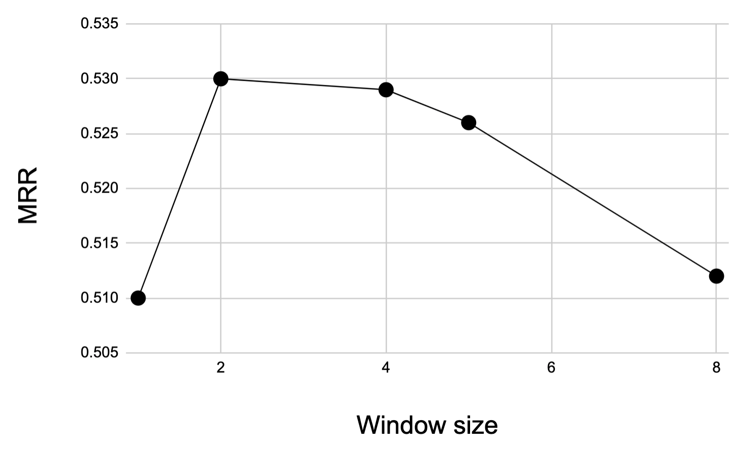
Figure 3: MRR of ReAlE for window sizes as the first five divisors of the embedding size (200) on JF17K.

8 Conclusion

In this work, we introduce ReAlE for reasoning in knowledge hypergraphs. To design a powerful method, we build on the primitives of relational algebra, which is the calculus of relational models. We prove that ReAlE can represent the primitive relational algebra operations renaming, projection, selection, set union, and set difference, and is fully expressive. The results of our experiments on real and synthetic datasets are consistent with the theoretical findings.

Appendix A Theoretical Analysis

The current section groups the theoretical analysis of our work into four parts. In particular, Section A.1 proves that ReAlE is fully expressive. Section A.2 proves that m-TransH, RAE, and NaLP are not fully expressive (G-MPNN scoring function and its non-expressiveness were discussed in Section 2 of the main paper). Section A.3 shows how closely ReAlE can represent relational algebra operations. Section A.4 further proves that HypE cannot represent all relational algebra operations (in particular, we show that HypE cannot represent selection).

For completeness, we restate the theorems and the scoring function. In what follows, we use lower case $x_{1},\dots,x_{n}$ to denote particular entities, $\bar{x}$ a sequence of particular entities, and $\mathbf{x}$ the embedding of $x$. Recall that our model embeds each entity $x_{i}$ into a vector $\mathbf{x_{i}}\in[0,1]^{d}$ of length $d$, and each relation $r$ into a matrix $\mathbf{r}\in\mathbb{R}^{|r|\times d}$. Recall that $w$ denotes the window size, $n_{w}=\lfloor\frac{d}{w}\rfloor$ the number of windows, and $b_{r}^{j}$ the bias term of relation $r$ for the $j^{th}$ window, for all $j=0,\dots,n_{w}-1$. Equation 10 defines ReAlE’s score of a tuple $r(x_{1},x_{2},\dots,x_{n})$, where $\sigma$ is a monotonically-increasing nonlinear function that is differentiable almost everywhere and $\theta$ is the set of all entity and relation embeddings.

$$\begin{split}&{\phi_{\theta}}(r(x_{1},\dots,x_{n}))=\\ &\frac{1}{n_{w}}\sum_{j=0}^{n_{w}-1}\sigma\left(b_{r}^{j}+\sum_{i=1}^{|r|}\sum_{k=0}^{w-1}\mathbf{x_{i}}[jw+k]\times\mathbf{r}[i][jw+k]\right)\end{split}$$ (10)

A.1 Full Expressivity of ReAlE

The following result proves that there exists a setting of the parameters for which ReAlE can separate true and false tuples for arbitrary input. In particular, we show it for the case where $\sigma$ is the sigmoid function.

Theorem 1 (Expressivity)

For any ground truth over entities $\mathcal{E}$ and relations $\mathcal{R}$ containing $\lambda$ true tuples with $\alpha=\max_{r\in{\mathcal{R}}}(|r|)$ as the maximum arity over all relations in $\mathcal{R}$, there is a ReAlE model with $n_{w}=\lambda$, $w=\alpha$, $d=\max(\alpha\lambda,\alpha)$, and $\sigma(x)=\frac{1}{1+\exp(-x)}$ that accurately separates the true tuples from the false ones.

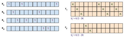
Figure 4: An example of a ReAlE embedding assignments for true tuples $\tau_{0}=r_{1}(x_{a},x_{b},x_{c})$, $\tau_{1}=r_{2}(x_{a},x_{c})$, $\tau_{2}=r_{1}(x_{c},x_{b},x_{d})$ and $\tau_{3}=r_{1}(x_{d},x_{c},x_{a})$. Here, the number of true tuples $\lambda=n_{w}=4$, maximum arity $\omega=3$. Cells that are set to zero are left empty for better readability. As an example, given that $x_{b}$ is in position $1$ of $\tau_{2}$, we set cell $2\times\omega+1=7$ of $x_{b}$ to $1$. We further set the value of $r_{1}$ at positions [$1$][$7$] to $K$.

Proof: Let $T=\{\tau_{0},\tau_{1},\dots,\tau_{\lambda-1}\}$ be all the true tuples defined over $\mathcal{E}$ and $\mathcal{R}$. To prove the theorem, we show an assignment of embedding values for each of the entities and relations in $T$ such that the scoring function of ReAlE is as follows.

$$\phi(\tau)\begin{cases}\geq\frac{1-\epsilon}{\lambda}&\text{if $\tau\in T$}\\ <\epsilon&\text{otherwise}\end{cases}$$

Here, $\epsilon$ is an arbitrary small value such that $\epsilon<\frac{1}{2+\lambda^{2}}$. Observe that $\lambda$ is a positive integer. Therefore, $\epsilon$ and $\frac{1-\epsilon}{\lambda}$ never meet.

We first consider the case where $\lambda>0$.

Let $K=2\times\sigma^{-1}(1-\epsilon)$. Then, $\sigma(\frac{K}{2})=1-\epsilon$ and $\sigma(\frac{-K}{2})=\epsilon$. We begin the proof by first describing an assignment of the embeddings of each of the entities and relations in ReAlE; we then proceed to show that with such an embedding, ReAlE accurately separates the true tuples from the false ones.

We consider the embeddings of entities to be $n_{w}=\lambda$ blocks of size $w$ each, such that each block $i$ is conceptually associated with true tuple $\tau_{i}$ for all $0\leq i<\lambda$. Then, for a given entity $x_{m}$ at position $m$ of tuple $\tau_{i}$, we set the value $\mathbf{x_{m}}[$iw + m$]$ to $1$, for all $0\leq i<\lambda$. All other values in $\mathbf{x_{m}}$ are set to zero. For the relation embeddings, first recall that these embeddings are matrices of dimension $|r|\times w\lambda$, and we consider each of the $|r|$ rows of this matrix to be $\lambda$ blocks of size $w$, where $|r|>1$ is the arity of the given relation. If a given relation $r$ appears in true tuple $\tau_{i}$, we set the $|r|$ values at position [$iw+k$][$iw+k$] to $K$, for all $0\leq k<|r|$ and $0\leq i<\lambda$; all other values in the relation embedding are set to zero. Finally, we set all the bias terms in our model to $b_{r}^{j}=\frac{K}{2}-|r|\times K$, for all $0\leq j<\lambda$. As an example, consider Figure 4, in which the first true tuple $\tau_{0}$ is defined on relation $r_{1}$; thus the embedding of $r_{1}$ has all ones in its first $3\times 3$ block (note that since $r_{1}$ is the relation in the third and fourth true tuples, then the third and fourth blocks of the embedding of $r_{1}$ are also filled with $1$s). $\tau_{0}$ has entity $x_{b}$ at its second position; hence the embedding of $x_{b}$ has a $1$ at its second position. We claim that with such an assignment, the score of tuples that are true is $\geq\frac{1-\epsilon}{\lambda}$ and $<\epsilon$ otherwise.

To see why this assignment works, first observe that our scoring function ${\phi_{\theta}}{}$ is an averaging of the sum of $\lambda$ sigmoids; each sigmoid is defined on an embedding block where we sum the bias term with the sum of pairwise product between the entity and relation embeddings of the given block.

Let $\tau_{p}=r(x_{1},\dots,x_{m})$ be a true tuple and observe the embeddings of its entities and relations. The blocks at position $p$ of the embeddings of each of $x_{1},\dots,x_{m}$ contain exactly one value $1$ each (with the rest being zero); and the block at position $p$ of the relation embedding for $r$ contains all $K$s. With such an assignment, the block at position $p$ will contribute the following sigmoid to the scoring function.

$$\sigma\left(b_{r}^{p}+|r|K\right)=\sigma\left(\frac{K}{2}-(|r|K)+(|r|K)\right)=\sigma\left(\frac{K}{2}\right)=1-\epsilon$$ (11)

All other blocks $q\neq p$ in $\tau_{p}$ contain at least one entity embedding block (for each of $x_{a},\dots,x_{m}$) to be all zeros (because otherwise they will be duplicate tuples in $T$). Assume that there are $c>0$ entity blocks that are all zeros for block $q$. Then, we have $|r|-c$ blocks that contain exactly one cell with value $1$, for all $0\leq q<\lambda$, $q\neq p$. Looking at $\tau_{0}$ in the example of Figure 4, if $q=1$ (second block), then $c=1$ since the second block of $x_{b}$ is all zeros.

Thus, any block $q$ in $\tau_{p}$ will contribute to the scoring function in one of two ways, depending on whether or not $r$ is a relation in $\tau_{q}$.

If $r$ happens to be a relation in $\tau_{q}$ (e.g. $r_{1}$ is a relation in $\tau_{0}$, $\tau_{2}$ and $\tau_{3}$ in Figure 4), then the $|r|\times w$-sized block at position $q$ of the relation embedding is all set to $K$; and since $c>1$,

$$\begin{split}&\sigma\left(b_{r}^{q}+(|r|-c)K\right)=\\ &\sigma\left(\frac{K}{2}-(|r|K)+(|r|-c)K\right)=\sigma\left(\frac{K}{2}-cK\right)<\epsilon\end{split}$$ (12)

If $r$ is not a relation in $\tau_{q}$, then the block at position $q$ of the relation embedding is all zeros. In this case,

$$\sigma\left(b_{r}^{q}+0\right)=\sigma\left(\frac{K}{2}-(|r|K)\right)<\epsilon$$ (13)

In the end, the score of any true tuple ${\phi_{\theta}}{}(\tau_{p})$ will be the sum of $\lambda$ sigmoids divided by $\lambda$ such that exactly one of these sigmoids (block at position $p$) has a value $1-\epsilon$, while the other $\lambda-1$ sigmoids $<\epsilon$. The score of a true tuple $\tau_{p}$ can thus be bounded as follows.

$${\phi_{\theta}}{(\tau_{p})}>=\frac{1-\epsilon}{\lambda}$$ (14)

In the case of a false tuple, all the sigmoids will yield values $<\epsilon$ (as they will be of the forms in either of Equations LABEL:eq:express_false_1, or 13). The score of a false tuple $\tau_{f}$ can thus be bounded as follows.

$${\phi_{\theta}}{(\tau_{f})}<\frac{\lambda\epsilon}{\lambda}=\epsilon$$ (15)

To complete the proof, we consider the case when $\lambda=0$. In this case, we let the entity and relation embeddings be blocks of arbitrary size and set all values to zero. We set the bias terms as before. Then, the score of any tuple will be ${\phi_{\theta}}{(\tau_{f})}<\epsilon$ (Equation 15), which is what we want. This completes the proof. $\Box$

A.2 Full Expressivity of Some Baselines

The following results prove that some of the baselines are not fully expressive and have severe restrictions on the types of relations they can model. Liu et al. (2020) discuss some of these limitations, and here we address them more formally.

Theorem 2

m-TransH, RAE, and NaLP are not fully expressive and have restrictions on the relations these approaches can represent.

The proof of the above theorem follows from Lemma 2.1 and Lemma 2.2 below.

Lemma 2.1

m-TransH and RAE are not fully expressive and have restriction on what relations these approaches can represent.

Proof: Kazemi & Poole (2018) prove that TransH (Wang et al., 2014) is not fully expressive and explore its restrictions. As m-TransH reduces to TransH for binary relations, it inherits all its restrictions and is not fully expressive. RAE also follows the same strategy as m-TransH in modeling the relations. Therefore, both m-TransH and RAE are not fully expressive. $\Box$

Lemma 2.2

NaLP is not fully expressive.

Proof: NaLP first concatenates the embeddings of entities and the embedding of their corresponding roles in the tuples, then applies to them the following functions: 1D convolution, projection layer, minimum, and another projection layer. Looking carefully at the output of the model, the NaLP scoring function for a tuple $r(x_{1},\dots,x_{n})$ is in the form of $|\mathbf{P_{1}}\mathbf{x_{1}}+\dots+\mathbf{P_{n}}\mathbf{x_{n}}+\mathbf{r}|_{1}$ with $\mathbf{P_{i}}$ as learnable diagonal matrices with some shared parameters. In the binary setup ($n=2$), the score function of NaLP is $|\mathbf{P_{1}}\mathbf{x_{1}}+\mathbf{P_{2}}\mathbf{x_{2}}+\mathbf{r}|_{1}$. Kazemi & Poole (2018), however, proved that translational methods having a score function of $|\mathbf{P_{1}}\mathbf{x_{1}}-\alpha\mathbf{P_{2}}\mathbf{x_{2}}+\mathbf{r}|_{i}$ are not fully expressive and have severe restrictions on what relations these approaches can represent. NaLP has the same score function with $\alpha=-1$ and $i=1$ and therefore is not fully expressive. $\Box$

A.3 Representing Relational Algebra with ReAlE

Theorem 3 (Renaming)

Given permutation function $\pi$, and relation $s$, there exists a parametrization for relation $t$ in ReAlE such that for entities $x_{1},\dots,x_{n}$, with arbitrary embeddings

$${\phi_{\theta}}(t(x_{1},\dots,x_{n}))={\phi_{\theta}}(s(x_{\pi(1)},x_{\pi(2)},\dots,x_{\pi(n)}))$$

Proof: To prove the above statement, we show that given entity embeddings $\mathbf{x_{1}},\dots,\mathbf{x_{n}}$ and an embedding for $s$, there exists a parametrization for $t$ that satisfies the above equality.

We claim that the following settings for $t$ are enough to show the theorem.

1. $\mathbf{t}[\pi(i)][k]=\mathbf{s}[i][k]~{}~{}~{}\forall~{}1\leq i\leq n,~{}\forall~{}0\leq k<d$, and

2. $b^{j}_{t}=b^{j}_{s}~{}~{}~{}\forall~{}0\leq j<n_{w}$

To see why, we simply expand the score function of $s$ and replace the values for $s$ by that of $t$ as described, to obtain the score for $t$.

$${\phi_{\theta}}(s(x_{\pi(1)},x_{\pi(2)},\dots,x_{\pi(n)}))=\frac{1}{n_{w}}\sum_{j=0}^{n_{w}-1}\sigma(b_{s}^{j}+\sum_{i=1}^{|s|}\sum_{k=0}^{w-1}\mathbf{x}_{\pi(i)}[j\times w+k]\times\mathbf{s}[i][j\times w+k])=\frac{1}{n_{w}}\sum_{j=0}^{n_{w}-1}\sigma(b_{t}^{j}+\sum_{i=1}^{|s|}\sum_{k=0}^{w-1}\mathbf{x}_{\pi(i)}[j\times w+k]\times\mathbf{t}[\pi(i)][j\times w+k])=\frac{1}{n_{w}}\sum_{j=0}^{n_{w}-1}\sigma(b_{t}^{j}+\sum_{i=1}^{|t|}\sum_{k=0}^{w-1}\mathbf{x}_{i}[j\times w+k]\times\mathbf{t}[i][j\times w+k])={\phi_{\theta}}(t(x_{1},x_{2},\dots,x_{n}))$$

$\Box$

Theorem 4 (Projection)

For any relation $s$ on $n$ arguments there exists a parametrization for relation $t$ on $m<n$ arguments in ReAlE such that for any arbitrary sequence $x_{1},\dots,x_{n}$

$${\phi_{\theta}}(t(x_{1},\dots,x_{m}))\geq{\phi_{\theta}}(s(x_{1},\dots,x_{n}))$$

Proof: To prove the above statement, we first expand the score function of each side of the inequality.

$${\phi_{\theta}}(t(x_{1},\dots,x_{m}))=\frac{1}{n_{w}}\sum_{j=0}^{n_{w}-1}\sigma(b_{t}^{j}+\sum_{i=1}^{m}\sum_{k=0}^{w-1}\mathbf{x}_{i}[j\times w+k]\times\mathbf{t}[i][j\times w+k])$$ (16)

$${\phi_{\theta}}(s(x_{1},\dots,x_{n}))={\frac{1}{n_{w}}\sum_{j=0}^{n_{w}-1}\sigma(b_{s}^{j}+\sum_{i=1}^{m}\sum_{k=0}^{w-1}\mathbf{x}_{i}[j\times w+k]\times\mathbf{s}[i][j\times w+k]}+~{}\sum_{i=m+1}^{n}\sum_{k=0}^{w-1}\mathbf{x}_{i}[j\times w+k]\times\mathbf{s}[i][j\times w+k])$$ (17)

The theorem holds with the following assignments.

1. $\mathbf{t}[i][k]=\mathbf{s}[i][k]~{}~{}~{}\forall~{}1\leq i\leq m,~{}\forall~{}0\leq k<d$, and

2. $b^{j}_{t}=b^{j}_{s}+\displaystyle\sum_{i=m+1}^{n}\sum_{k=0}^{w-1}\max(0,\mathbf{s}[i][k])~{}~{}~{}\forall~{}0\leq j<n_{w}$

$\Box$

Theorem 5 (Selection 1)

For arbitrary relation $s$, there exists a parametrization for relation $t$ in ReAlE such that for arbitrary entities $x_{1},\dots,x_{n-1}$

$${\phi_{\theta}}(t(x_{1},\dots,x_{n-1}))={\phi_{\theta}}(s(x_{1},\dots,x_{n-1},x_{n-1}))\\$$

Proof: To prove the above statement, we first expand the score function of ${\phi_{\theta}}$ for the right side of the equality.

$$\begin{split}&{\phi_{\theta}}(s(x_{1},\dots,x_{n-1},x_{n-1}))\\ =&\frac{1}{n_{w}}\sum_{j=0}^{n_{w}-1}\sigma(b_{s}^{j}+\sum_{i=1}^{n-2}\sum_{k=0}^{w-1}\mathbf{x}_{i}[j\times w+k]\times\mathbf{s}[i][j\times w+k]\\ &+\sum_{k=0}^{w-1}\mathbf{x}_{n-1}[j\times w+k]\times\mathbf{s}[n-1][j\times w+k]\\ &+\sum_{k=0}^{w-1}\mathbf{x}_{n-1}[j\times w+k]\times\mathbf{s}[n][j\times w+k])\\ =&~{}(\text{grouping terms})\\ &\frac{1}{n_{w}}\sum_{j=0}^{n_{w}-1}\sigma(b_{s}^{j}+\sum_{i=1}^{n-2}\sum_{k=0}^{w-1}\mathbf{x}_{i}[j\times w+k]\times\mathbf{s}[i][j\times w+k]\\ &+{\sum_{k=0}^{w-1}\mathbf{x}_{n-1}[j\times w+k]\times(\mathbf{s}[n-1][j\times w+k]}+\mathbf{s}[n][j\times w+k]))\end{split}$$ (18)

For the lemma to hold, the above score has to be equal to that of $t$, which is described as follws.

$${\phi_{\theta}}(t(x_{1},\dots,x_{n-1}))={\frac{1}{n_{w}}\sum_{j=0}^{n_{w}-1}\sigma(b_{t}^{j}+\sum_{i=1}^{n-2}\sum_{k=0}^{w-1}\mathbf{x}_{i}[j\times w+k]\times\mathbf{t}[i][j\times w+k]}+{\sum_{k=0}^{w-1}\mathbf{x}_{n-1}[j\times w+k]\times\mathbf{t}[n-1][j\times w+k])}$$ (19)

The scores in Equations 18 and 19 are equal when the embedding and bias of $t$ are set as follows.

1. $\mathbf{t}[i][k]=\mathbf{s}[i][k]~{}~{}~{}\forall~{}1\leq i\leq n-2,~{}\forall~{}0\leq k<d$, and

2. $\mathbf{t}[n-1][k]=\mathbf{s}[n-1][k]+\mathbf{s}[n][k]~{}~{}~{}~{}\forall~{}0\leq k<d$, and

3. $b^{j}_{t}=b^{j}_{s}~{}~{}~{}\forall~{}0\leq j<n_{w}$

$\Box$

Theorem 6 (Selection 2)

For arbitrary relation $s$ and for a fixed constant $c$, there exists a parametrization for relation $t$ in ReAlE such that for arbitrary entities $x_{1},\dots,x_{n-1}$

$${\phi_{\theta}}(t(x_{1},\dots,x_{n-1}))={\phi_{\theta}}(s(x_{1},\dots,x_{n-1},c))$$

Proof: Using similar score expansions as in the proof of Lemma 5, we can rewrite the scores of the two relations as follows.

$$\begin{split}&{\phi_{\theta}}(s(x_{1},\dots,x_{n-1},c))\\ &=\frac{1}{n_{w}}\sum_{j=0}^{n_{w}-1}\sigma(b_{s}^{j}+\sum_{i=1}^{n-2}\sum_{k=0}^{w-1}\mathbf{x}_{i}[j\times w+k]\times\mathbf{s}[i][j\times w+k]\\ &+\sum_{k=0}^{w-1}\mathbf{x}_{n-1}[j\times w+k]\times\mathbf{s}[n-1][j\times w+k]\\ &+\sum_{k=0}^{w-1}\mathbf{c}[j\times w+k]\times\mathbf{s}[n][j\times w+k])\end{split}$$ (20)

$${{\phi_{\theta}}(t(x_{1},\dots,x_{n-1}))}=\frac{1}{n_{w}}\sum_{j=0}^{n_{w}-1}\sigma(b_{t}^{j}+{\sum_{i=1}^{n-2}\sum_{k=0}^{w-1}\mathbf{x}_{i}[j\times w+k]\times\mathbf{t}[i][j\times w+k]}+{\sum_{k=0}^{w-1}\mathbf{x}_{n-1}[j\times w+k]\times\mathbf{t}[n-1][j\times w+k])}$$ (21)

The scores in Equations 20 and 21 are equal when the embedding and bias of $t$ are as set follows.

1. $\mathbf{t}[i][k]=\mathbf{s}[i][k]~{}~{}~{}\forall~{}1\leq i\leq n-1,~{}\forall~{}0\leq k<d$, and

2. $b^{j}_{t}=b^{j}_{s}+\sum_{k=0}^{w-1}\mathbf{s}[n][j\times w+k]\times\mathbf{c}[j\times w+k]~{}~{}~{}\forall~{}0\leq j<n_{w}$

$\Box$

Theorem 7 (Set Union)

For arbitrary relations $s$ and $r$ with the same arity, there exists a parametrization for relation $t$ in ReAlE such that for arbitrary entity set $\bar{x}$

$${\phi_{\theta}}(t(\bar{x}))\geq\max({\phi_{\theta}}(s(\bar{x})),{\phi_{\theta}}(r(\bar{x})))$$

Proof: Given that ReAlE embeds entities in non-negative vectors and examining the scoring functions of each of the relations $t$, $r$, $s$, it can be observed that the above inequality holds by setting the following values.

1. $t[i][k]=\max(s[i][k],r[i][k])$     $\forall~{}~{}1\leq i<|\bar{x}|$ and $0\leq k<d$.

2. $b^{j}_{t}=\max(b^{j}_{s},b^{j}_{r})$     $\forall~{}~{}0\leq j<n_{w}$.

$\Box$

In the lemma that follows, recall that the relation complement function (if it exists) is some linear function $f({\phi_{\theta}}(r({\bar{x}})))={\phi_{\theta}}(\neg r({\bar{x}}))$ for arbitrary relation $r$ and entities $\bar{x}$ that also has the form $f(\sigma(x))=\sigma(c\times x)$ with $c$ as a constant. For instance, when $\sigma$ is sigmoid, $f(x)=1-x$ and $c=-1$ ($f(\sigma(x))=1-\sigma(x)=\sigma(-x)$) and when $\sigma$ is tanh, $f(x)=-x$ and $c=-1$ ($f(\sigma(x))=-\sigma(x)=\sigma(-x)$).

Theorem 8 (Set Difference)

For arbitrary relations $r$ and $s$ with the same arity, if $f$ is a linear relation complement function and $f(\sigma(x))=\sigma(c\times x)$ with $c$ as a constant, there exists a parametrization for relation $t$ in ReAlE such that for arbitrary entities $x_{1},\dots,x_{n}$

$${\phi_{\theta}}(t(\bar{x}))\leq\min({\phi_{\theta}}(s(\bar{x})),f({\phi_{\theta}}(r(\bar{x}))))$$

Proof:

As $f$ is the relation complement, we have:

$${\phi_{\theta}}(\neg r(x_{1},\dots,x_{n}))=f({\phi_{\theta}}(r(x_{1},\dots,x_{n})))$$

As $f$ is linear, we can distribute it inside the summation as follows:

$$f({\phi_{\theta}}(r(x_{1},\dots,x_{n})))=\frac{1}{n_{w}}\sum_{j=0}^{n_{w}-1}f(\sigma(b_{r}^{j}+\sum_{i=1}^{|r|}\sum_{k=0}^{w-1}\mathbf{x_{i}}[jw+k]\times\mathbf{r}[i][jw+k]))$$

Now, as $f(\sigma(x))=\sigma(c\times x)$, we can distribute it inside the $\sigma$ as follows:

$$f({\phi_{\theta}}(r(x_{1},\dots,x_{n})))=\frac{1}{n_{w}}\sum_{j=0}^{n_{w}-1}\sigma\left(b_{r}^{j}\times c+\sum_{i=1}^{|r|}\sum_{k=0}^{w-1}\mathbf{x_{i}}[jw+k]\times\mathbf{r}[i][jw+k]\right\times c)$$

Therefore, for the above inequality to hold, the bias terms and embedding values of $t$ must be at most that of each of $s$ and the complement of the score of $r$. Examining the scoring functions of each of the relations $t$, $r$, $s$, it can be observed that the lemma holds when the following is set.

1. $t[i][k]=\min(s[i][k],r[i][k]\times c)$     $\forall~{}~{}1\leq i<|\bar{x}|$ and $0\leq k<d$.

2. $b^{j}_{t}=\min(b^{j}_{s},b^{j}_{r}\times c)$     $\forall~{}~{}0\leq j<n_{w}$.

$\Box$

A.4 Representing Relational Algebra with HypE

So far, we showed that ReAlE is fully expressive and can represent the relational algebra operations renaming, projection, selection, set union, and set difference. We also showed that most other models for knowledge hypergraph completion are not fully expressive. In this section, we show that even as HypE is fully expressive in general, it cannot represent some relational algebra operations (namely, selection) while at the same time retaining its full expressivity. In special cases, such as when all tuples are false, it obviously can, however, we show that in the general case it cannot.

We proceed by first showing in Theorem 9 that HypE cannot represent selection for arbitrary entity and relation embeddings while retaining full expressivity. Now, one might think that even if representing selection is not possible for all embeddings, there might be some embedding space for which HypE would be able to represent selection. In Theorem 10 we show that when the embedding size is less than the number of entities (as it usually is the case), then there is no setting for which HypE would be able to represent selection.

Recall that HypE embeds an entity $x_{i}$ and a relation $r$ in vectors $\mathbf{x_{i}}\in\mathbb{R}^{d}$ and $\mathbf{r}\in\mathbb{R}^{d}$ respectively, where $d$ be the embedding size. In what follows, we let $f(x,p)$ be a function that computes the convolution of the embedding of entity $x$ with the corresponding convolution filters associated to position $p$ and outputs a vector (see (Fatemi et al., 2020) for more details). We let ${\phi_{\theta}^{H}}{}$ to be the HypE scoring function.

Theorem 9 (HypE Selection 1 (a))

For arbitrary relation $s$ and arbitrary embeddings for entities $x_{1},\dots,x_{n-1}$, there exists no parametrization for relation $t$ in HypE such that

$${\phi_{\theta}^{H}}(t(x_{1},\dots,x_{n-1}))={\phi_{\theta}^{H}}(s(x_{1},\dots,x_{n-1},x_{n-1}))\\$$ (22)

Proof:

To see why there is no parametrization for $t$ that satisfies Equation (22), we first expand the left and right hand side of the equality as follows.

$${\phi_{\theta}^{H}}(t(x_{1},\dots,x_{n-1}))={\phi_{\theta}^{H}}(s(x_{1},\dots,x_{n-1},x_{n-1}))\\$$

$$\begin{split}&\sum_{i=1}^{d}\mathbf{t}[i]\times f(x_{1},1)[i]\times\dots\times f(x_{n-1},n-1)[i]=\\ &\sum_{i=1}^{d}\mathbf{s}[i]\times f(x_{1},1)[i]\times\dots\times f(x_{n-1},n-1)[i]\times f(x_{n-1},n)[i]\end{split}$$

For this equation to hold, the following should hold for arbitrary entities $x_{1},\dots,x_{n-1}$, and $\forall~{}~{}1\leq i\leq d$.

$$or\begin{cases}f(x_{1},1)[i]\times\dots\times f(x_{n-1},n-1)[i]=0\\ \mathbf{t}[i]=\mathbf{s}[i]\times f(x_{n-1},n)[i]\end{cases}$$ (23)

For an entity $x$ at position $p$ in a tuple, the output of function $f(x,p)$ depends on the embedding of entity $x$ and the convolution filters associated with position $p$. Note that these convolution filters are shared among all relations in the knowledge hypergraph and are not specific to relation $s$ or $t$.

As we want Equation (23) to hold for arbitrary entity embeddings, it is easy to see that there exists at least one setup for convolution filters and entity embeddings for which none of the factors in the product $f(x_{i},1)[i]\times\dots\times f(x_{n-1},n-1)[i]$ is zero.

Now consider such an embedding setting. The only way Equation (23) is satisfied is when we set $\mathbf{t}[i]=\mathbf{s}[i]\times f(x_{n-1},n)[i]$ for all $1\leq i\leq d$. Observe that by setting the embedding of relation $t$ to the embedding of $s$ times $f(x_{n-1},n)$ for a particular entity $x_{n-1}$, we have effectively set it to a fixed value. Now consider an entity $x_{k}$ such that $f(x_{k},n)\neq f(x_{n-1},n)$, and apply the selection $t$ to $x_{k}$ by replacing $x_{n-1}$ with $x_{k}$ in Equation (22). The equality condition in the equation will not hold, because none of the conditions in Equation (23) hold. Therefore, in this setup, $t$ fails to represent $s$ for arbitrary entity embeddings.

Given that relation $t$ should represent selection of $s$ for all the entities in the hypergraph, setting it to a fixed value will make it incapable of representing selection for arbitrary entities. We can thus conclude that there is no parametrization for HypE such that it can represent selection for arbitrary embeddings of relations and entities. $\Box$

We now show that when the embedding size is less than the number of entities $|{\mathcal{E}}|$ in the hypergraph, there is no setting for which HypE would be able to represent selection without losing full expressivity.

Theorem 10 (HypE Selection 1 (b))

For arbitrary relation $s$, there exists no parametrization for relation $t$ in HypE having scoring function ${\phi_{\theta}^{H}}$ such that for arbitrary entities $x_{1},\dots,x_{n}$ and embedding dimension $d<|{\mathcal{E}}|$, where $|{\mathcal{E}}|$ is the number of entities in the knowledge hypergraph, HypE remains fully expressive and

$${\phi_{\theta}^{H}}(t(x_{1},\dots,x_{n-1}))={\phi_{\theta}^{H}}(s(x_{1},\dots,x_{n-1},x_{n-1}))\\$$

Proof:

Consider $|s|=2$ and $|t|=1$ and tuples $t(x_{j})$ and $s(x_{j},x_{j})$ such that relation $t$ is a selection of $s$. We will show that when the embedding dimension $d$ of the entities is smaller than the number of entities in the knowledge hypergraph, there is no parametrization of HypE that gets $t$ to represent $s$ while retaining full expressivity.

For the sake of contradiction, assume that the lemma statement is false. Then there exists a parametrization for $t$ such that HypE is fully expressive and that

$${\phi_{\theta}^{H}}(t(x_{j}))={\phi_{\theta}^{H}}(s(x_{j},x_{j}))$$

Expanding the score function for $s$ and $t$ we get

$$\sum_{i=1}^{d}\mathbf{t}[i]\times f(x_{j},1)[i]=\sum_{i=1}^{d}\mathbf{s}[i]\times f(x_{j},1)[i]\times f(x_{j},2)[i]$$

$$\Rightarrow\sum_{i=1}^{d}f(x_{j},1)[i]\times\left(\mathbf{t}[i]-\mathbf{s}[i]\times f(x_{j},2)[i]\right)=0$$

For this equation to hold for arbitrary entities $x_{1},x_{2},\dots,x_{n}$, it should hold for all $1\leq i\leq d$ and all $1\leq j\leq|{\mathcal{E}}|$ for which $\mathbf{s}(x_{j},x_{j})$ is true. Assuming that $d<|{\mathcal{E}}|$, we need to have the following hold for all $1\leq j\leq|{\mathcal{E}}|$ and $1\leq i\leq d$.

$$or\begin{cases}f(x_{j},1)[i]=0\\ \mathbf{t}[i]=\mathbf{s}[i]\times f(x_{j},2)[i]\\ \end{cases}$$ (24)

We claim that to satisfy the above equation simultaneously for all possible $i$ and $j$, there must be at least one entity $x_{k}$ for which the convolution function returns a zero vector; that is, $f(x_{k},1)[i]=0$ for all $0\leq i\leq d$. To see why this is true, assume the contrary; that is, for each convolution filter $f(x_{j},1)$ has at least one bit that is different than zero for arbitrary entity $x_{j}$. Without loss of generality, let the $j$th bit $f(x_{j},1)[j]=K_{j}$, for all $1\leq j\leq|{\mathcal{E}}|$ and $K_{j}\in\mathcal{R^{*}}$. Then, to satisfy Equation 24 at index $j$, we must set $\mathbf{t}[j]=\mathbf{s}[j]\times f(x_{j},2)[j]$. As Equation 24 must be satisfied for all entities, then all other entities $x_{k}$ with $k\neq j$ must have their $j$-th bit set to zero. Thus $f(x_{k},1)[j]=0$ for all $0\leq j\leq d$ and $j\neq k$. See Figure 5. Since we have $d<|{\mathcal{E}}|$, and by the pigeon-hole principle, there must be at least one entity $x_{d+1}$ such that $f(x_{d+1},1)=0$ for all $1\leq i\leq d$. This contradicts the original assumption, and thus there exists at least one $k$ for which $f(x_{k},1)$ returns a zero vector.

This would further imply that any tuple having $x_{k}$ in the first position will have a score ${\phi_{\theta}^{H}}{}$ of zero. This would be regardless of the relation in the tuple, or whether or not it is true. This violates the full-expressivity of HypE, thus contradicting the original assumption that the lemma statement is False. Therefore, when $d<|{\mathcal{E}}|$, there is no parametrization for $t$ such that HypE represents selection while retaining full expressivity. $\Box$

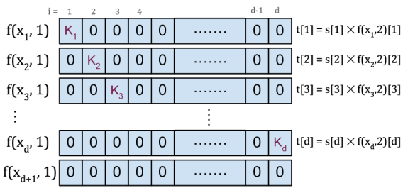
Figure 5: Proof of Theorem 10: If at least one value of each vector $f(x_{i},1)$ is different than zero ($K_{i}$ ¿ 0) and the value of at most one position $i$ can be non-zero (the $d$ columns in the figure), then by the pigeon-hole principle, we will run out of indices as we have more entities in the knowledge hypergraph. In the above image, the entity $x_{d+1}.$

Appendix B Datasets

B.1 Public Dataset Statistics

Table 3 summarizes the statistics for the public knowledge hypergraph datasets JF17K, FB-auto, and m-FB15K.

Table 3: Dataset Statistics.

			number of tuples			number of tuples with respective arity
Dataset	$|\mathcal{E}|$	$|\mathcal{R}|$	#train	#valid	#test	#arity=2	#arity=3	#arity=4	#arity=5	#arity=6
JF17K	29,177	327	77,733	–	24,915	56,322	34,550	9,509	2,230	37
FB-auto	3,410	8	6,778	2,255	2,180	3,786	0	215	7,212	0
m-FB15K	10,314	71	415,375	39,348	38,797	82,247	400,027	26	11,220	0

B.2 Synthetic Dataset

To study and evaluate the generalization power of hypergraph completion models in a controlled environment, we generate a synthetic dataset called REL-ER (RELational Erdős-Rényi). To create REL-ER, we build on the Erdős-Rényi model (Erdős & Rényi, 1959) for generating random graphs and extend it to knowledge hypergraphs. In what follows, we discuss the details of our algorithm.

B.2.1 Knowledge Hypergraphs

A knowledge hypergraph is a directed hypergraph $H=(V,E,R)$ with nodes (entities) $V$, edges (tuples) $E$, and edge labels (relations) $R$ such that:

• every edge in the hypergraph consists of an ordered sequence of nodes,

• every edge has a label $r_{i}\in R$, and

• edges with the same label are defined on the same number of nodes.

Observe that in knowledge hypergraphs, edges having the same label form a uniform directed hypergraph (all edges defined on the same number of nodes). We can thus think of $H$ as the combination of $|R|$ directed uniform hypergraphs.

B.2.2 Extending Erdős-Rényi to Knowledge Hypergraphs

In the Erdős-Rényi model, all graphs with a fixed number of nodes and edges are equally likely. Equivalently, in such a random graph, each edge is present in the graph with a fixed probability $p$, independent of other edges. In this section, we describe a method of generating a random knowledge hypergraph inspired by the Erdős-Rényi process.

Let $n$ be the (predefined) number of nodes in the hypergraph and $n_{r}$ be the number of relations. We let $R$ be a list of relations defined in terms of arity and a probability that influences the number of tuples generated for that given relation. More formally,

$$R=\{(k_{i},p_{i})|k_{i}=arity,0\leq p_{i}\leq 1,\forall i=0,\dots,n_{r}\}$$

The expected number of edges generated for a given relation $r_{i}$ is $m_{i}=k_{i}!{n\choose k_{i}}p_{i}$. As the process of including edges in the graph is a Binomial, we can compute this expected value by sampling from the following probability density.

$$P(m_{i})={N\choose{m_{i}}}p_{i}(1-p_{i})^{N-m_{i}}$$

where $N=k_{i}!{n\choose k_{i}}$ is the number of possible $k_{i}$-uniform (directed) edges in the hypergraph.

The running time of Algorithm 2 depends on the number of nodes $n$ and the arity $k_{i}$ of each relation. Let $\displaystyle k=max_{k_{i}\in R}k_{i}$. Thus the running time of Algorithm 2 is $O(|R|n^{k})$.

Algorithm 2 generate_knowledge_hypergraph($V$, $R$))

  edge_list = []

  $n$ = len($V$)

  for $r$, ($k$, $p$) in enumerate(R) do

     $N=k!{n\choose k}$

     $m$ = random.binomial($N$, $p$) {result of flipping a coin $N$ times with probability of success $p$}

     edge_count = 0

     while edge_count $<=m$ do

        edge = random.sample($V$, $k$) {select $k$ vertices from $V$ at random}

        if edge not in edge_list then

           edge_list.append([$r$] + edge)

           edge_count = edge_count + 1

        end if

     end while

  end for

  return edge_list

B.2.3 Dataset Generation

To evaluate a model on how well it represents relational algebra operations, we generate a set of ground-truth true tuples, each of which is the result of repeated application of a primary relational algebra operation to an existing tuple (hyperedge). The operations we are interested in are renaming, projection, selection, set union and set difference.

  $E$ = generate_knowledge_hypergraph($V$, $R$)

  for $i$ in $range(n\_derived\_tuples)$ do

     $op$ = randomly select one primary operation

     $tuple$ = randomly select one hyperedge from $E$

     apply $op$ to $tuple$

     add $tuple$ to the set of edges $E$

  end for

Algorithm 3 generate_ground_truth($V$, $R$, $n\_derived\_tuples$)

Finally, the complete algorithm to generate the train, valid, and test sets of the synthetic dataset is described in Algorithm 4 below.

Algorithm 4 synthesize_dataset($V$, $R$, $n\_derived\_tuples$)

  $ground\_truth$ = generate_ground_truth($V$, $R$,                          $n\_derived\_tuples$)

  $relational\_data$ = sub-sample from $ground\_truth$

  train, valid, test = randomly split $relational\_data$ into train, valid and test

Appendix C Implementation Details

We implement ReAlE in PyTorch (Paszke et al., 2019) and use Adagrad (Duchi et al., 2011) as the optimizer and dropout (Srivastava et al., 2014) to regularize the model. We perform early stopping and hyperparameter tuning based on the MRR on the validation set. We fix the maximum number of epochs to $1000$ and batch size to $128$. We set the embedding size and negative ratio to $200$ and $10$ respectively. We tune $lr$ (learning rate) and $w$ (window size) using the sets $\{0.05,0.08,0.1,0.2\}$, and $\{1,2,4,5,8\}$ (first five divisors of 200). We tune $\sigma$ (nonlinear function) using the set $\{tanh,sigmoid,exponent\}$ for the JF17K dataset. The results of the different nonlinear functions are in Table 4. As $sigmoid$ outperforms the $tanh$ and $exponent$, we only tried $sigmoid$ for other datasets.

Reported results for the baselines on JF17K, FB-AUTO, and M-FB15K are taken from the original paper except for that of GETD (Liu et al., 2020). The original paper of GETD only reports results for arity 3 and 4 as trained and tested separately in the corresponding arity. However, in our experimental setup, we train and test in a dataset containing relations of different arities. For that, we train and test GETD. As GETD learns a tensor of dimension $|r|$ for each relation $r$, it needs $d^{|r|}$ (with $d$ as embedding size) number of parameters. The original paper proposes smart strategies to reduce the number of parameters to be learned by the model. However, we still need to store the relation embedding and thus need to store $d^{|r|}$ floating-point numbers for each relation $r$. Because of our memory limitation ($16$GB GPU), we could only train the GETD model for embedding size of less than $10$.

The sign “-” in Table 1 indicates that the corresponding paper has not provided the results.

For the experiment on the synthetic dataset, we compare our model with m-TransH (Wen et al., 2016) and HypE (Fatemi et al., 2020), which are the only competitive baselines that have provided the code (https://github.com/ElementAI/HypE, https://github.com/wenjf/multi-relational_learning).

The code and the data for all the experiments is available at https://github.com/baharefatemi/ReAlE.

Table 4: Knowledge hypergraph completion results for ReAlE on JF17K for different $\sigma$ (nonlinear function).

	JF17K
Model	MRR	Hit@1	Hit@3	Hit@10
ReAlE ($\sigma$ as exponent) (Ours)	0.394	0.311	0.428	0.548
ReAlE ($\sigma$ as tanh) (Ours)	0.512	0.430	0.548	0.667
ReAlE ($\sigma$ as sigmoid) (Ours)	0.530	0.454	0.563	0.677

References

- Balažević et al. (2019) Balažević, I., Allen, C., and Hospedales, T. M. Tucker: Tensor factorization for knowledge graph completion. arXiv preprint arXiv:1901.09590, 2019.
- Battaglia et al. (2018) Battaglia, P. W., Hamrick, J. B., Bapst, V., Sanchez-Gonzalez, A., Zambaldi, V., Malinowski, M., Tacchetti, A., Raposo, D., Santoro, A., Faulkner, R., et al. Relational inductive biases, deep learning, and graph networks. arXiv preprint arXiv:1806.01261, 2018.
- Bollacker et al. (2008) Bollacker, K., Evans, C., Paritosh, P., Sturge, T., and Taylor, J. Freebase: a collaboratively created graph database for structuring human knowledge. In ACM ICMD, 2008.
- Bordes et al. (2013) Bordes, A., Usunier, N., Garcia-Duran, A., Weston, J., and Yakhnenko, O. Translating embeddings for modeling multi-relational data. In NIPS, 2013.
- Côté et al. (2018) Côté, M.-A., Kádár, Á., Yuan, X., Kybartas, B., Barnes, T., Fine, E., Moore, J., Hausknecht, M., El Asri, L., Adada, M., et al. Textworld: A learning environment for text-based games. In Workshop on Computer Games, pp. 41–75. Springer, 2018.
- Duchi et al. (2011) Duchi, J., Hazan, E., and Singer, Y. Adaptive subgradient methods for online learning and stochastic optimization. JMLR, 12(Jul):2121–2159, 2011.
- Erdős & Rényi (1959) Erdős, P. and Rényi, A. On random graphs. Publicationes Mathematicae Debrecen, 6:290–297, 1959.
- Fatemi et al. (2020) Fatemi, B., Taslakian, P., Vazquez, D., and Poole, D. Knowledge hypergraphs: Prediction beyond binary relations. In IJCAI, 2020.
- Feng et al. (2019) Feng, Y., You, H., Zhang, Z., Ji, R., and Gao, Y. Hypergraph neural networks. In AAAI, 2019.
- Guan et al. (2019) Guan, S., Jin, X., Wang, Y., and Cheng, X. Link prediction on n-ary relational data. In The World Wide Web Conference, pp. 583–593, 2019.
- Guan et al. (2020) Guan, S., Jin, X., Guo, J., Wang, Y., and Cheng, X. Neuinfer: Knowledge inference on n-ary facts. In Proceedings of the 58th Annual Meeting of the Association for Computational Linguistics, pp. 6141–6151, 2020.
- Hitchcock (1927) Hitchcock, F. L. The expression of a tensor or a polyadic as a sum of products. Journal of Mathematics and Physics, 6(1-4):164–189, 1927.
- Johnson et al. (2017) Johnson, J., Hariharan, B., van der Maaten, L., Fei-Fei, L., Lawrence Zitnick, C., and Girshick, R. Clevr: A diagnostic dataset for compositional language and elementary visual reasoning. In Proceedings of the IEEE Conference on Computer Vision and Pattern Recognition, pp. 2901–2910, 2017.
- Kadlec et al. (2017) Kadlec, R., Bajgar, O., and Kleindienst, J. Knowledge base completion: Baselines strike back. In RepL4NLP, 2017.
- Kazemi & Poole (2018) Kazemi, S. M. and Poole, D. Simple embedding for link prediction in knowledge graphs. In NIPS, 2018.
- Lacroix et al. (2018) Lacroix, T., Usunier, N., and Obozinski, G. Canonical tensor decomposition for knowledge base completion. ICML, 2018.
- Liu et al. (2020) Liu, Y., Yao, Q., and Li, Y. Generalizing tensor decomposition for n-ary relational knowledge bases. In Proceedings of The Web Conference 2020, pp. 1104–1114, 2020.
- Paszke et al. (2019) Paszke, A., Gross, S., Massa, F., Lerer, A., Bradbury, J., Chanan, G., Killeen, T., Lin, Z., Gimelshein, N., Antiga, L., Desmaison, A., Kopf, A., Yang, E., DeVito, Z., Raison, M., Tejani, A., Chilamkurthy, S., Steiner, B., Fang, L., Bai, J., and Chintala, S. Pytorch: An imperative style, high-performance deep learning library. In NeurIPS. 2019.
- Raedt et al. (2016) Raedt, L. D., Kersting, K., Natarajan, S., and Poole, D. Statistical relational artificial intelligence: Logic, probability, and computation. Synthesis Lectures on Artificial Intelligence and Machine Learning, 10(2):1–189, 2016.
- Rosso et al. (2020) Rosso, P., Yang, D., and Mauroux, P. C. Beyond triplets: hyper-relational knowledge graph embedding for link prediction. In Proceedings of The Web Conference 2020, pp. 1885–1896, 2020.
- Sinha et al. (2020) Sinha, K., Sodhani, S., Pineau, J., and Hamilton, W. L. Evaluating logical generalization in graph neural networks. arXiv preprint arXiv:2003.06560, 2020.
- Srivastava et al. (2014) Srivastava, N., Hinton, G., Krizhevsky, A., Sutskever, I., and Salakhutdinov, R. Dropout: a simple way to prevent neural networks from overfitting. JMLR, 15(1):1929–1958, 2014.
- Teru et al. (2020) Teru, K., Denis, E., and Hamilton, W. Inductive relation prediction by subgraph reasoning. In International Conference on Machine Learning, pp. 9448–9457. PMLR, 2020.
- Wang et al. (2014) Wang, Z., Zhang, J., Feng, J., and Chen, Z. Knowledge graph embedding by translating on hyperplanes. In AAAI, 2014.
- Wen et al. (2016) Wen, J., Li, J., Mao, Y., Chen, S., and Zhang, R. On the representation and embedding of knowledge bases beyond binary relations. In IJCAI, 2016.
- Yadati (2020) Yadati, N. Neural message passing for multi-relational ordered and recursive hypergraphs. Advances in Neural Information Processing Systems, 33, 2020.
- Yadati et al. (2018) Yadati, N., Nimishakavi, M., Yadav, P., Louis, A., and Talukdar, P. Hypergcn: Hypergraph convolutional networks for semi-supervised classification. arXiv preprint arXiv:1809.02589, 2018.
- Zhang et al. (2018) Zhang, R., Li, J., Mei, J., and Mao, Y. Scalable instance reconstruction in knowledge bases via relatedness affiliated embedding. In Proceedings of the 2018 World Wide Web Conference, pp. 1185–1194, 2018.