Linear Functions to the Extended Reals

Abstract

This note investigates functions from $\mathbb{R}^{d}$ to $\mathbb{R}\cup\{\pm\infty\}$ that satisfy axioms of linearity wherever allowed by extended-value arithmetic. They have a nontrivial structure defined inductively on $d$, and unlike finite linear functions, they require $\Omega(d^{2})$ parameters to uniquely identify. In particular they can capture vertical tangent planes to epigraphs: a function (never $-\infty$) is convex if and only if it has an extended-valued subgradient at every point in its effective domain, if and only if it is the supremum of a family of “affine extended” functions. These results are applied to the well-known characterization of proper scoring rules, for the finite-dimensional case: it is carefully and rigorously extended here to a more constructive form. In particular it is investigated when proper scoring rules can be constructed from a given convex function.

1 Introduction

The extended real number line, denoted $\overline{\mathbb{R}}=\mathbb{R}\cup\{\pm\infty\}$, is widely useful particularly in convex analysis. But I am not aware of an answer to the question: What would it mean to have a “linear” $f:\mathbb{R}^{d}\to\overline{\mathbb{R}}$? The extended reals have enough structure to hope for a useful answer, but differ enough from a vector space to need investigation. A natural approach is that $f$ must satisfy the usual linearity axioms of homogeneity and additivity whenever legal under extended-reals arithmetic. Here is an example when $d=3$:

$$f(x,y,z)=\begin{cases}\text{if $z>0$}&\rightarrow~{}~{}\infty\\ \text{if $z<0$}&\rightarrow~{}~{}-\infty\\ \text{if $z=0$}&\rightarrow~{}~{}\begin{cases}\text{if $y>0$}&\rightarrow~{}~{}\infty\\ \text{if $y<0$}&\rightarrow~{}~{}-\infty\\ \text{if $y=0$}&\rightarrow~{}~{}x.\end{cases}\end{cases}$$

We will see that all linear extended functions (Definition 2.1) on $\mathbb{R}^{d}$ have the above inductive format, descending dimension-by-dimension until reaching a finite linear function (Proposition 2.5). In fact, a natural representation of this procedure is parsimonious, requiring as many as $\Omega(d^{2})$ real-valued parameters to uniquely identify an extended linear function on $\mathbb{R}^{d}$ (Proposition 2.6). This structure raises the possibility, left for future work, that linear extended functions are significantly nontrivial on infinite-dimensional spaces.

Linear extended functions arise naturally as extended subgradients (Definition 3.1) of a convex function $g$. These can be used to construct affine extended functions (Definition 3.4) capturing vertical supporting hyperplanes to convex epigraphs. Along such a hyperplane, intersected with the boundary of the domain, $g$ can sometimes have the structure of an arbitrary convex function in $d-1$ dimensions. For example, the above $f$ is an extended subgradient, at the point $(1,0,0)$, of the discontinuous convex function

$$g(x,y,z)=\begin{cases}\text{if $z>0$}&\rightarrow~{}~{}\infty\\ \text{if $z<0$}&\rightarrow~{}~{}0\\ \text{if $z=0$}&\rightarrow~{}~{}\begin{cases}\text{if $y>0$}&\rightarrow~{}~{}\infty\\ \text{if $y<0$}&\rightarrow~{}~{}0\\ \text{if $y=0$}&\rightarrow~{}~{}\frac{1}{2}x^{2}.\end{cases}\end{cases}$$

A proper function (one that is never $-\infty$) is convex if and only if it has an extended subgradient at every point in its effective domain (Proposition 3.10). We also find it is convex if and only if it is the pointwise supremum of affine extended functions (Proposition 3.7).

Proper scoring rules.

The motivation for this investigation was the study of scoring rules: functions $S$ assigning a score $S(p,y)$ to any prediction $p$ (a probability distribution over outcomes) and observed outcome $y$. This $S$ is called proper if reporting the true distribution of the outcome maximizes expected score. A well-known characterization states that proper scoring rules arise as and only as subgradients of convex functions (McCarthy, 1956; Savage, 1971; Schervish, 1989).

Modern works (Gneiting and Raftery, 2007; Frongillo and Kash, 2014) generalize this characterization to allow scores of $-\infty$, corresponding to convex functions that are not subdifferentiable. These works therefore replace subgradients with briefly-defined generalized “subtangents”, but they slightly sidestep the questions tackled head-on here: existence of these objects and their roles in convex analysis. So these characterizations are not fully constructive. In particular, it may surprise even experts that rigorous answers are not available to the following questions, given a convex function $g$: (a) under what conditions can one construct a proper scoring rule from it? (b) when is the resulting scoring rule strictly proper? (c) do the answers depend on which subgradients of $g$ are used, when multiple choices are available?

Section 4 uses the machinery of extended linear functions to prove a “construction of proper scoring rules” that answers such questions for the finite-outcome case.

First, Theorem 4.9 allows predictions to range over the entire simplex. It implies a slightly-informal claim of Gneiting and Raftery (2007), Section 3.1: Any convex function on the probability simplex gives rise to a proper scoring rule (using any choices of its extended subgradients). Furthermore, it shows that a strictly convex function can only give rise to strictly proper scoring rules and vice versa. These facts are likely known by experts in the community; however, I do not know of formal claims and proofs. This may be because, when scoring rules can be $-\infty$, proofs seem to require significant formalization and investigation of “subtangents”. In this paper, this investigation is supplied by linear extended functions and characterizations of (strictly) convex functions as those that have (uniquely supporting) extended subgradients everywhere.

Next, Theorem 4.15 allows prediction spaces $\mathcal{P}$ to be any subset of the simplex. It sharpens the characterizations of Gneiting and Raftery (2007); Frongillo and Kash (2014) by showing $S$ to be proper if and only if it can be constructed from extended subgradients of a convex $g$ that is interior-locally-Lipschitz (Definition 4.13). It also answers the construction questions (a)-(c) above, e.g. showing that given such a $g$, some but not necessarily all selections of its extended subgradients give rise to proper scoring rules.

Preliminaries.

Functions in this work are defined on Euclidean spaces of dimension $d\geq 0$. I ask the reader’s pardon for abusing notation slightly: I use $\mathbb{R}^{d}$ refer to any such space. For example, I may argue that a certain function exists on domain $\mathbb{R}^{d}$, then refer to that function as being defined on a given $d$-dimensional subspace of $\mathbb{R}^{d+1}$.

Let $g:\mathbb{R}^{d}\to\overline{\mathbb{R}}$. The effective domain $\textrm{effdom}\mathopen{}\mathclose{{}\left(g}\right)$ of $g$ is $\{x\in\mathbb{R}^{d}~{}:~{}g(x)\neq\infty\}$. The function $g$ is convex if its epigraph $\{(x,y)\in\mathbb{R}^{d}\times\mathbb{R}:y\geq g(x)\}$ is a convex set. Equivalently, it is convex if for all $x,x^{\prime}\in\textrm{effdom}\mathopen{}\mathclose{{}\left(g}\right)$ and all $0<\rho<1$, $g(\rho\cdot x+(1-\rho)x^{\prime})\leq\rho g(x)+(1-\rho)g(x^{\prime})$, observing that this sum may contain $-\infty$ but not $+\infty$. It is strictly convex on a convex set $\mathcal{P}\subseteq\textrm{effdom}\mathopen{}\mathclose{{}\left(g}\right)$ if the previous inequality is always strict for $x,x^{\prime}\in\mathcal{P}$ with $x\neq x^{\prime}$.

We say a function $h$ minorizes $g$ if $h(x)\leq g(x)$ for all $x$. $\textrm{cl}\mathopen{}\mathclose{{}\left(A}\right)$ denotes the closure of the set $A$ and $\textrm{int}\mathopen{}\mathclose{{}\left(A}\right)$ its interior. For $a\in\overline{\mathbb{R}}$, the sign function is $\textrm{sign}(a)=1$ if $a>0$, $\textrm{sign}(a)=0$ if $a=0$, and $\textrm{sign}(a)=-1$ if $a<0$.

The extended reals.

The extended reals, $\overline{\mathbb{R}}=\mathbb{R}\cup\{\pm\infty\}$, have the following rules of arithmetic for any $\alpha,\beta\in\mathbb{R}$: $\beta+\infty=\infty$, $\beta-\infty=-\infty$, and

$$\alpha\cdot\infty=\begin{cases}\infty&\alpha>0\\ 0&\alpha=0\\ -\infty&\alpha<0.\end{cases}$$

Illegal and disallowed is addition of $\infty$ and $-\infty$. Addition is associative and commutative as long as it is legal; multiplication of multiple scalars and possibly one non-scalar is associative and commutatitve. Multiplication by a scalar distributes over legal sums.

$\overline{\mathbb{R}}$ has the following rules of comparison: $-\infty<\beta<\infty$ for every $\beta\in\mathbb{R}$. The supremum of a subset of $\overline{\mathbb{R}}$ is $\infty$ if it contains $\infty$ or it contains an unbounded-above set of reals; the analogous facts hold for the infimum. Also, $\inf\emptyset=\infty$ and $\sup\emptyset=-\infty$. I will not put a topology on $\overline{\mathbb{R}}$ in this work.

2 Linear extended functions

The following definition makes sense with a general real vector space $\mathcal{X}$ in place of $\mathbb{R}^{d}$, but it remains to be seen if all results can extend.

Definition 2.1.

Call the function $f:\mathbb{R}^{d}\to\overline{\mathbb{R}}$ a linear extended function if:

1. (scaling) For all $x\in\mathbb{R}^{d}$ and all $\alpha\in\mathbb{R}$: $f(\alpha x)=\alpha f(x)$.

2. (additivity) For all $x,x^{\prime}\in\mathbb{R}^{d}$: If $f(x)+f(x^{\prime})$ is legal, i.e. $\{f(x),f(x^{\prime})\}\neq\{\pm\infty\}$, then $f(x+x^{\prime})=f(x)+f(x^{\prime})$.

If the range of $f$ is included in $\mathbb{R}$, Definition 2.1 reduces to the usual definition of a linear function. For clarity, this paper may emphasize the distinction by calling such $f$ finite linear.

To see that this definition can be satisfied nontrivially, let $f_{1},f_{2}:\mathbb{R}^{d}\to\mathbb{R}$ be finite linear and consider $f(x):=\infty\cdot f_{1}(x)+f_{2}(x)$. With a representation $f_{1}(x)=v_{1}\cdot x$, we have

$$f(x)=\begin{cases}\infty&v_{1}\cdot x>0\\ -\infty&v_{1}\cdot x<0\\ f_{2}(x)&v_{1}\cdot x=0.\end{cases}$$

Claim 2.2.

Any such $f$ is a linear extended function.

Proof.

Multiplication by a scalar distributes over the legal sum $\infty\cdot f_{1}(x)+f_{2}(x)$, so $\alpha f(x)=\infty\cdot f_{1}(\alpha x)+f_{2}(\alpha x)=f(\alpha x)$. To obtain additivity of $f$, consider cases on the pair $(v_{1}\cdot x,~{}v_{1}\cdot x^{\prime})$. If both are zero, $f(x+x^{\prime})=f_{2}(x+x^{\prime})=f_{2}(x)+f_{2}(x^{\prime})=f(x)+f(x^{\prime})$. If they have opposite signs, then $\{f(x),f(x^{\prime})\}=\{\pm\infty\}$ and the requirement is vacuous. If one is positive and the other nonnegative, then $v_{1}\cdot(x+x^{\prime})>0$, so we have $f(x+x^{\prime})=\infty=f(x)+f(x^{\prime})$. The remaining case, one negative and the other nonpositive, is exactly analogous. ∎

Such $f$ are not all the linear extended functions, because the subspace where $x\cdot v_{1}=0$ need not be entirely finite-valued. As in the introduction’s example, it can itself be divided into infinite and neg-infinite open halfspaces, with $f$ finite only on some further-reduced subspace. We will show that all linear extended functions can be constructed in this recursive way, Algorithm 1 (heavily relying on the setting of $\mathbb{R}^{d}$).

Algorithm 1 Computing a linear extended function $f:\mathbb{R}^{d}\to\overline{\mathbb{R}}$

  Parameters: $t\in\{0,\ldots,d\}$; finite linear $\hat{f}:\mathbb{R}^{d-t}\to\mathbb{R}$; if $t\geq 1$, unit vectors $v_{1}\in\mathbb{R}^{d},\ldots,v_{t}\in\mathbb{R}^{d-t+1}$

  Input: $x\in\mathbb{R}^{d}$

  for $j=1,\ldots,t$ do

     if $v_{j}\cdot x>0$ then

        return $\infty$

     else if $v_{j}\cdot x<0$ then

        return $-\infty$

     end if

     reparameterize $x$ as a vector in $\mathbb{R}^{d-j}$, a member of the subspace $\{x^{\prime}~{}:~{}v_{j}\cdot x^{\prime}=0\}$

  end for

  return $\hat{f}(x)$

For the following lemma, recall that a subset $S$ of $\mathbb{R}^{d}$ is a convex cone if, when $x,x^{\prime}\in S$ and $\alpha,\beta>0$, we have $\alpha x+\beta x^{\prime}\in S$. A convex cone need not contain $\vec{0}$.

Lemma 2.3 (Decomposition).

$f:\mathbb{R}^{d}\to\overline{\mathbb{R}}$ is linear extended if and only if: (1) the sets $S^{+}=f^{-1}(\infty)$ and $S^{-}=f^{-1}(-\infty)$ are convex cones with $S^{+}=-S^{-}$, and (2) the set $F=f^{-1}(\mathbb{R})$ is a subspace of $\mathbb{R}^{d}$, and (3) $f$ coincides with some finite linear function on $F$.

Proof.

$(\implies)$ Let $f$ be linear extended. The scaling axiom implies $f(\vec{0})=0$, so $\vec{0}\in F$. Observe that $F$ is closed under scaling (by the scaling axiom) and addition (the addition axiom is never vacuous on $x,x^{\prime}\in F$). So it is a subspace. $f$ satisfies scaling and additivity (never vacuous) for all members of $F$, so it is finite linear there. This proves (2) and (3). Next: the scaling axiom implies that if $x\in S^{+}$ then $-x\in S^{-}$, giving $S^{+}=-S^{-}$ as claimed. Now let $x,x^{\prime}\in S^{+}$ and $\alpha,\beta>0$. The scaling axiom implies $\alpha x$ and $\beta x^{\prime}$ are in $S^{+}$. The additivity axiom implies $\alpha x+\beta x^{\prime}\in S^{+}$, proving it is a convex cone. We immediately get $S^{-}=-S^{+}$ is a convex cone as well, proving (1).

$(\impliedby)$ Suppose $F$ is a subspace on which $f$ is finite linear and $S^{+}=-S^{-}$ is a convex cone. We prove $f$ satisfies the two axioms needed to be linear extended. First, $F$ includes $\vec{0}$ by virtue of being a subspace (inclusion of $\vec{0}$ is also implied by $S^{+}=-S^{-}$, because $S^{+}\cap S^{-}=\emptyset$). Because $f$ is finite linear on $F$, $f(\vec{0})=0$. We now show $f$ satisfies the two axioms of linearity.

For scaling, if $x\in F$, the axiom follows from closure of $F$ under scaling and finite linearity of $f$ on $F$. Else, let $\alpha\in\mathbb{R}$ and $x\in S^{+}$ (the case $x\in S^{-}$ is exactly analogous). If $\alpha>0$, then $\alpha x\in S^{+}$ because it is a convex cone, which gives $f(\alpha x)=\alpha f(x)=\infty$. If $\alpha=0$, then $f(\alpha x)=\alpha f(x)=0$. If $\alpha<0$, then use that $-x\in S^{-}$ by assumption, and since $S^{-}$ is a cone and $-\alpha>0$, we have $(-\alpha)(-x)\in S^{-}$. In other words, $f(\alpha x)=-\infty=\alpha f(x)$, as required.

For additivity, let $x,x^{\prime}$ be given.

• If $x,x^{\prime}\in F$, additivity follows from closure of $F$ under addition and finite linearity of $f$ on $F$.

• If $x,x^{\prime}\in S^{+}$, then $x+x^{\prime}\in S^{+}$ as required because it is a convex cone; analogously for $x,x^{\prime}\in S^{-}$.

• If $x\in S^{+},x^{\prime}\in S^{-}$ or vice versa, the axiom is vacuously satisfied.

The remaining case is, without loss of generality, $x\in S^{+},x^{\prime}\in F$ (the proof is identical for $x\in S^{-},x^{\prime}\in F$). We must show $x+x^{\prime}\in S^{+}$. Because $F$ is a subspace and $x^{\prime}\in F,x\not\in F$, we must have $x+x^{\prime}\not\in F$. Now suppose for contradiction that $x+x^{\prime}\in S^{-}$. We have $-x\in S^{-}$ because $S^{-}=-S^{+}$. Because $S^{-}$ is a convex cone, it is closed under addition, so $x+x^{\prime}+(-x)=x^{\prime}\in S^{-}$, a contradiction. So $x+x^{\prime}\in S^{+}$. ∎

Lemma 2.4 (Recursive definition).

$f:\mathbb{R}^{d}\to\overline{\mathbb{R}}$ is linear extended if and only if one of the following hold:

1. $f$ is finite linear (this case must hold if $d=0$), or

2. There exists a unit vector $v_{1}$ and linear extended function $f_{2}$ on the $d-1$ dimensional subspace $\{x~{}:~{}v_{1}\cdot x=0\}$ such that $f(x)=f_{2}(x)$ if $x\cdot v_{1}=0$, else $f(x)=\infty\cdot\textrm{sign}(v_{1}\cdot x)$.

Proof.

$(\implies)$ Suppose $f$ is linear extended. The case $d=0$ is immediate, as $f(\vec{0})=0$ by the scaling axiom. So let $d\geq 1$ and suppose $f$ is not finite linear; we show case (2) holds. Let $S^{+}=f^{-1}(\infty)$, $S^{-}=f^{-1}(-\infty)$, and $F=f^{-1}(\mathbb{R})$. Recall from Lemma 2.3 that $F$ is a subspace, necessarily of dimension $<d$ by assumption that $f$ is not finite; meanwhile $S^{+}=-S^{-}$ and both are convex cones.

We first claim that there is an open halfspace on which $f(x)=\infty$, i.e. included in $S^{+}$. First, $\textrm{cl}\mathopen{}\mathclose{{}\left(S^{+}}\right)$ includes a closed halfspace: if not, the set $\textrm{cl}\mathopen{}\mathclose{{}\left(S^{+}}\right)\cup\textrm{cl}\mathopen{}\mathclose{{}\left(S^{-}}\right)\neq\mathbb{R}^{d}$ and then its complement, an open set, would necessarily have affine dimension $d$ yet would be included in $F$, a contradiction. Now, because $S^{+}$ is convex, it includes the relative interior of $\textrm{cl}\mathopen{}\mathclose{{}\left(S^{+}}\right)$, so it includes an open halfspace.

Write this open halfspace $\{x~{}:~{}v_{1}\cdot x>0\}$ for some unit vector $v_{1}$. Because $S^{-}=-S^{+}$, we have $f(x)=-\infty$ on the complement $\{x~{}:~{}v_{1}\cdot x<0\}$. Let $f_{2}$ be the restriction of $f$ to the remaining subspace, $\{x~{}:~{}v_{1}\cdot x=0\}$. This set is closed under addition and scaling, and $f$ satisfies the axioms of a linear extended function, so $f_{2}$ is a linear extended function as well.

$(\impliedby)$ If case (1) holds and $f$ is finite linear, then it is immediately linear extended as well, QED. In case (2), we apply Lemma 2.3 to $f_{2}$. We obtain that it is finite linear on a subspace of $\{x~{}:~{}v_{1}\cdot x=0\}$, which is a subspace of $\mathbb{R}^{d}$, giving that $f$ is finite linear on a subspace. We also obtain $f_{2}^{-1}(\infty)=-f_{2}^{-1}(-\infty)$ and is a convex cone. It follows directly that $f^{-1}(\infty)=-f^{-1}(-\infty)$. In fact, $f^{-1}(\infty)=f_{2}^{-1}(\infty)\cup\{x~{}:~{}v_{1}\cdot x>0\}$. The first set is a convex cone lying in the closure of the second set, also a convex cone. So the union is a convex cone: scaling is immediate; any nontrivial convex combination of a point from each set lies in the second, giving convexity; scaling and convexity give additivity. This shows that $f^{-1}(\infty)$ is a convex cone, the final piece needed to apply Lemma 2.3 and declare $f$ linear extended. ∎

Proposition 2.5 (Correctness of Algorithm 1).

A function $f:\mathbb{R}^{d}\to\overline{\mathbb{R}}$ is linear extended if and only if it is computed by Algorithm 1 for some $t\in\{0,\ldots,d\}$, some $v_{1}\in\mathbb{R}^{d},\ldots,v_{t}\in\mathbb{R}^{d-t+1}$, and some finite linear $\hat{f}:\mathbb{R}^{d}\to\mathbb{R}$.

Proof.

$(\implies)$ Suppose $f$ is linear extended. By Lemma 2.4, there are two cases. If $f$ is finite linear, then take $t=0$ and $\hat{f}=f$ in Algorithm 1. Otherwise, Lemma 2.4 gives a unit vector $v_{1}$ so that $f(x)=\infty$ if $v_{1}\cdot x>0$ and $f(x)=-\infty$ if $v_{1}\cdot x<0$, as in Algorithm 1. $f$ is linear extended on $\{x~{}:~{}v_{1}\cdot x=0\}$, so we iterate the procedure until reaching a subspace where $f$ is finite linear, setting $t$ to be the number of iterations.

$(\impliedby)$ Suppose $f$ is computed by Algorithm 1. We will use the two cases of Lemma 2.4 to show $f$ is linear extended. If $t=0$, then $f$ is finite linear, hence linear extended (case 1). If $t\geq 1$, then $f$ is in case 2 with unit vector $v_{1}$ and function $f_{2}$ equal to the implementation of Algorithm 1 on $t-1$, $\hat{f}$, and $v_{2},\dots,v_{t}$. This proves by induction on $t$ that, if $f$ is computed by Algorithm 1, then it satisfies one of the cases of Lemma 2.4, so it is linear extended. ∎

Proposition 2.6 (Parsimonious parameterization).

Each linear extended function has a unique representation by the parameters of Algorithm 1.

Proof.

For $i\in\{1,2\}$, let $f^{(i)}$ be the function computed by Algorithm 1 with the parameters $t^{(i)}$, $\hat{f}^{(i)}$, $\{v_{j}^{(i)}~{}:~{}j=1,\dots,t^{(i)}\}$. We will prove that $f^{(1)}$ and $f^{(2)}$ are distinct if any of their parameters differ: i.e. if $t^{(1)}\neq t^{(2)}$, or else $\hat{f}^{(1)}\neq\hat{f}^{(2)}$, or else there exists $j$ with $v_{j}^{(1)}\neq v_{j}^{(2)}$.

By Lemma 2.3, each $f^{(i)}$ is finite linear on a subspace $F^{(i)}$ and positive (negative) infinite on a convex cone $S^{i,+}$ (respectively, $S^{i,-}$) with $S^{i,+}=-S^{i,-}$. It follows that they are equal if and only if: $S^{1,+}=S^{2,+}$ (this implies $F^{(1)}=F^{(2)}$) and they coincide on $F^{(1)}$.

If $t^{(1)}\neq t^{(2)}$, then the dimensions of $F^{(1)}$ and $F^{(2)}$ differ, so they are nonequal, so $S^{1,+}\neq S^{2,+}$ and the functions are not the same. So suppose $t^{(1)}=t^{(2)}$. Now suppose the unit vectors are not the same, i.e. there is some smallest index $j$ such that $v^{(1)}_{j}\neq v^{(2)}_{j}$. Observe that on iteration $j$ of the algorithm, the $d-j+1$ dimensional subspace under consideration is identical for $f^{(1)}$ and $f^{(2)}$. But now there is some $x$ with $v^{(1)}_{j}\cdot x>0$ while $v^{(2)}_{j}\cdot x<0$, for example, $x=v^{(1)}_{j}-v^{(2)}_{j}$. On this $x$ (parameterized as a vector in $\mathbb{R}^{d}$), $f^{(1)}(x)=\infty$ while $f^{(2)}(x)=-\infty$, so the functions differ.

Finally, suppose $t^{(1)}=t^{(2)}$ and all unit vectors are the same. Observe that $F^{(1)}=F^{(2)}$. But if $\hat{f}^{(1)}\neq\hat{f}^{(2)}$, then there is a point in $F^{(1)}$ where $\hat{f}^{(1)}$ and $\hat{f}^{(2)}$ differ. On this point (parameterized as a vector in $\mathbb{R}^{d}$), $f^{(1)}$ and $f^{(2)}$ differ. ∎ One corollary is the following definition:

Definition 2.7 (Depth).

Say the depth of a linear extended function $f$ is the value of $t$ in its parameterization of Algorithm 1 (shown in Proposition 2.6 to be unique).

Another is that, while finite linear functions on $\mathbb{R}^{d}$ are uniquely identified by $d$ real-valued parameters, linear extended functions require as many as ${d\choose 2}+1=\Omega(d^{2})$: Unit vectors in $\mathbb{R}^{k}$ require $k-1$ parameters (for $k\geq 2$), so even assuming depth $t=d-1$, identifying the unit vectors takes $d-1+\cdots+1={d\choose 2}$ parameters, and one more defines $\hat{f}:\mathbb{R}\to\mathbb{R}$.

By the way, we would be remiss in forgetting to prove:

Proposition 2.8 (Convexity).

Linear extended functions are convex.

Proof.

We prove convexity by showing the epigraph of a linear extended function $f:\mathbb{R}^{d}\to\overline{\mathbb{R}}$ is convex. By induction on $d$: If $d=0$, then $f$ is finite linear (Lemma 2.4), so it has a convex epigraph. Otherwise, let $d\geq 1$. If $f$ is finite linear, then again it has a convex epigraph, QED. Otherwise, by Lemma 2.4, its epigraph is $A\cup B$ where: $A=\{x:v_{1}\cdot x<0\}$ for some unit vector $v_{1}\in\mathbb{R}^{d}$; and $B$ is the epigraph (appropriately reparameterized) of a linear extended function $f_{2}:\mathbb{R}^{d-1}\to\overline{\mathbb{R}}$ on the set $\{x:v_{1}\cdot x=0\}$. We have $B\subseteq\textrm{cl}\mathopen{}\mathclose{{}\left(A}\right)$, and both sets are convex (by inductive hypothesis), so their union is convex: any nontrivial convex combination of points lies in the interior of $A$. ∎ The effective domain of a linear extended function at least includes an open halfspace. If the depth is zero, it is $\mathbb{R}^{d}$; if the depth is $1$, it is a closed halfspace $\{x~{}:~{}v_{1}\cdot x\leq 0\}$, and otherwise it is neither a closed nor open set.

Structure.

It seems difficult to put useful algebraic or topological structure on the set of linear extended functions on $\mathbb{R}^{d}$. For example, addition of two functions is typically undefined. Convergence in the parameters of Algorithm 1 does not seem to imply pointwise convergence of the functions, as for instance we can have a sequence $v_{1}^{(m)}\to v_{1}$ such that members of $\{x~{}:~{}v_{1}\cdot x=0\}$ are always mapped to $\infty$. But perhaps future work can put a creative structure on this set.

3 Extended subgradients

Recall that a subgradient of a function $g$ at a point $x_{0}$ is a (finite) linear function $f$ satisfying $g(x)\geq g(x_{0})+f(x-x_{0})$ for all $x$. The following definition of extended subgradient replaces $f$ with a linear extended function; to force sums to be legal, we will only define it at points in the effective domain of a “proper” function, i.e. one that is never $-\infty$. A main aim of this section is to show that a proper function is convex if and only if it has an extended subgradient everywhere in its effective domain (Proposition 3.10).

Definition 3.1 (Extended subgradient).

Given a function $g:\mathbb{R}^{d}\to\mathbb{R}\cup\{\infty\}$, a linear extended function $f$ is an extended subgradient of $g$ at a point $x_{0}$ in its effective domain if, for all $x\in\mathbb{R}^{d}$, $g(x)\geq g(x_{0})+f(x-x_{0})$.

Again for clarity, if this $f$ is a finite linear function, we may call it a finite subgradient of $g$. Note that the sum appearing in Definition 3.1 is always legal because $g(x_{0})\in\mathbb{R}$ under its assumptions.

As is well-known, finite subgradients correspond to supporting hyperplanes of the epigraphs of convex functions $g$, but they do not exist at points where all such hyperplanes are vertical; consider, in one dimension,

$$g(x)=\begin{cases}0&x<1\\ 1&x=1\\ \infty&x>1.\end{cases}$$ (1)

We next show that every $g$ has an extended subgradient everywhere in its effective domain. For example, $f(z)=\infty\cdot z$ is an extended subgradient of the above $g$ at $x=1$.

Proposition 3.2 (Existence of extended subgradients).

Each convex function $g:\mathbb{R}^{d}\to\mathbb{R}\cup\{\infty\}$ has an extended subgradient at every point in its effective domain.

Proof.

Let $x$ be in the effective domain $G$ of $g$; we construct an extended subgradient $f_{x}$. The author finds the following approach most intuitive: Define $g_{x}(z)=g(x+z)-g(x)$, the shift of $g$ that moves $(x,g(x))$ to $(\vec{0},0)$. Let $G_{x}=\textrm{effdom}\mathopen{}\mathclose{{}\left(g_{x}}\right)$. Now we appeal to a technical lemma, Lemma 3.3 (next), which says there exists a linear extended $f_{x}$ that minorizes $g_{x}$. This completes the proof: For any $x^{\prime}\in\mathbb{R}^{d}$, we have $f_{x}(x^{\prime}-x)\leq g_{x}(x^{\prime}-x)$, which rearranges to give $g(x)+f_{x}(x^{\prime}-x)\leq g(x^{\prime})$ (using that $g(x)\in\mathbb{R}$ by assumption). ∎

Lemma 3.3.

Let $g_{x}:\mathbb{R}^{d}\to\mathbb{R}\cup\{\infty\}$ be a convex function with $g_{x}(\vec{0})=0$. Then there exists a linear extended function $f_{x}$ with $f_{x}(z)\leq g_{x}(z)$ for all $z\in\mathbb{R}^{d}$.

Proof.

First we make Claim (*): if $\vec{0}$ is in the interior of the effective domain $G_{x}$ of $g_{x}$, then such an $f_{x}$ exists. This follows because $g_{x}$ necessarily has at $\vec{0}$ a finite subgradient (Rockafellar (1970), Theorem 23.4), which we can take to be $f_{x}$.

Now, we prove the result by induction on $d$.

If $d=0$, then it is only possible to have $f_{x}=g_{x}$.

If $d\geq 1$, there are two cases. If $\vec{0}$ is in the interior of $G_{x}$, then Claim (*) applies and we are done.

Otherwise, $\vec{0}$ is in the boundary of the convex set $G_{x}$. This implies that there exists a hyperplane supporting $G_{x}$ at $\vec{0}$. That is, there is some unit vector $v\in\mathbb{R}^{d}$ such that $G_{x}\subseteq\{z~{}:~{}v\cdot z\leq 0\}$. Set $f_{x}(z)=\infty$ if $v\cdot z>0$ and $f_{x}(z)=-\infty$ if $v\cdot z<0$. Note $f_{x}$ minorizes $g$ on these regions, in the first case because $g_{x}(z)=\infty=f_{x}(z)$ (by definition of effective domain), and in the second case because $f_{x}(z)=-\infty$.

So it remains to define $f_{x}$ on the subspace $S:=\{z~{}:~{}v\cdot z=0\}$ and show that it minorizes $g_{x}$ there. But $g_{x}$, restricted to this subspace, is again a proper convex function equalling $0$ at $\vec{0}$, so by induction we have a minorizing linear extended function $\hat{f_{x}}$ on this $d-1$ dimensional subspace. Define $f_{x}(z)=\hat{f_{x}}(z)$ for $z\in S$. Then $f_{x}$ minorizes $g_{x}$ everywhere. We also have that $f_{x}$ is linear extended by Lemma 2.4, as it satisfies the necessary recursive format. ∎ This proof would have gone through if Claim (*) used “relative interior” rather than interior, because supporting hyperplanes also exist at the relative boundary. That version would have constructed extended subgradients of possibly lesser depth (Definition 2.7).

It is now useful to define affine extended functions. Observe that a bad definition would be “a linear extended function plus a constant.” Both vertical and horizontal shifts of linear extended functions must be allowed in order to capture, e.g.

$$h(x)=\begin{cases}-\infty&x<1\\ 1&x=1\\ \infty&x>1.\end{cases}$$ (2)

Definition 3.4 (Affine extended function).

A function $h:\mathbb{R}^{d}\to\overline{\mathbb{R}}$ is affine extended if for some $\beta\in\mathbb{R}$ and $x_{0}\in\mathbb{R}^{d}$ and some linear extended $f:\mathbb{R}^{d}\to\overline{\mathbb{R}}$ we have $h(x)=f(x-x_{0})+\beta$.

Definition 3.5 (Supports).

An affine extended function $h$ supports a function $g:\mathbb{R}^{d}\to\overline{\mathbb{R}}$ at a point $x_{0}\in\mathbb{R}^{d}$ if $h(x_{0})=g(x_{0})$ and for all $x\in\mathbb{R}^{d}$, $h(x)\leq g(x)$.

For example, the above $h$ in Display 2 supports, at $x_{0}=1$, the previous example $g$ of Display 1. Actually, $h$ supports $g$ at all $x_{0}\geq 1$.

Observation 3.6.

Given $\beta,x_{0},f$, define the affine extended function $h(x)=f(x-x_{0})+\beta$.

1. $h$ is convex: its epigraph is a shift of a linear extended function’s.

2. Let $g:\mathbb{R}^{d}\to\mathbb{R}\cup\{\infty\}$ such that $x_{0}\in\textrm{effdom}\mathopen{}\mathclose{{}\left(g}\right)$. Then $h$ supports $g$ at $x_{0}$ if and only if $f$ is an extended subgradient of $g$ at $x_{0}$.

3. If $h(x_{1})$ is finite, then for all $x$ we have $h(x)=f(x-x_{1})+\beta_{1}$ where $\beta_{1}=f(x_{1}-x_{0})+\beta$.

Point 2 follows because $h$ supports $g$ at $x_{0}$ if and only if $\beta=g(x_{0})$ and $g(x)\geq\beta+f(x-x_{0})$ for all $x$. Point 3 follows because $h(x_{1})=f(x_{1}-x_{0})+\beta$, so $f(x_{1}-x_{0})$ is finite: the sum $f(x-x_{1})+f(x_{1}-x_{0})$ is always legal and equals $f(x-x_{0})$.

An important fact in convex analysis is that a closed (i.e. lower semicontinuous) convex function $g$ is the pointwise supremum of a family of affine functions. We have the following analogue.

Proposition 3.7 (Supremum characterization).

A function $g:\mathbb{R}^{d}\to\mathbb{R}\cup\{\infty\}$ is convex if and only if it is the pointwise supremum of a family of affine extended functions.

Proof.

$(\impliedby)$ Let $H$ be a family of affine extended functions and let $g(x):=\sup_{h\in H}h(x)$. The epigraph of each affine extended function is a convex set (Observation 3.6), and $g$’s epigraph is the intersection of these, hence a convex set, so $g$ is convex.

$(\implies)$ Suppose $g$ is convex; let $H$ be the set of affine extended functions minorizing $g$. We show $g(x)=\sup_{h\in H}h(x)$.

First consider $x$ in the effective domain $G$ of $g$. By Proposition 3.2, $g$ has an extended subgradient at $x$, which implies (Observation 3.6) it has a supporting affine function $h_{x}$ there, and of course $h_{x}\in H$. We have $g(x)=h_{x}(x)$ and by definition $g(x)\geq h(x)$ for all $h\in H$, so $g(x)=\max_{h\in H}h(x)$.

Finally, let $x\not\in G$. We must show that $\sup_{h\in H}h(x)=\infty$. We apply a technical lemma, Lemma 3.8 (stated and proven next), to obtain a set $H^{\prime}$ of affine extended functions that all equal $-\infty$ on $G$ (hence $H^{\prime}\subseteq H$), but for which $\sup_{h\in H^{\prime}}h(x)=\infty$, as required. ∎

Lemma 3.8.

Let $G$ be a convex set in $\mathbb{R}^{d}$ and let $x\not\in G$. There is a set $H^{\prime}$ of affine extended functions such that $\sup_{h\in H^{\prime}}h(x)=\infty$ while $h(x^{\prime})=-\infty$ for all $h\in H$ and $x^{\prime}\in G$.

For intuition, observe that the easiest case is if $x\not\in\textrm{cl}\mathopen{}\mathclose{{}\left(G}\right)$, when we can use a strongly separating hyperplane to get a single $h$ that is $\infty$ at $x$ and $-\infty$ on $G$. The most difficult case is when $x$ is an extreme, but not exposed, point of $\textrm{cl}\mathopen{}\mathclose{{}\left(G}\right)$. (Picture a convex $g$ with effective domain $\textrm{cl}\mathopen{}\mathclose{{}\left(G}\right)$; now modify $g$ so that $g(x)=\infty$.) Capturing this case requires the full recursive structure of linear extended functions.

Proof.

Let $G^{\prime}=\{x^{\prime}-x~{}:~{}x^{\prime}\in G\}$. Note that $G^{\prime}$ is a convex set not containing $\vec{0}$. By Lemma 3.9, next, there is a linear extended function $f$ equalling $-\infty$ on $G^{\prime}$. Construct $H=\{h(x^{\prime})=f(x^{\prime}-x)+\beta~{}:~{}\beta\in\mathbb{R}\}$. Then $\sup_{h\in H}h(x)=\sup_{\beta\in\mathbb{R}}\beta=\infty$, while for $x^{\prime}\in G$ we have $h(x^{\prime})=f(x^{\prime}-x)+\beta=-\infty$. This proves Lemma 3.8. ∎

Lemma 3.9.

Given a convex set $G^{\prime}\subseteq\mathbb{R}^{d}$ not containing $\vec{0}$, there exists a linear extended $f$ with $f(x^{\prime})=-\infty$ for all $x^{\prime}\in G^{\prime}$.

Proof.

Note that if $G^{\prime}=\emptyset$, then the claim is immediately true; and if $d=0$, then $G^{\prime}$ must be empty. Now by induction on $d$: If $d=1$, then we can choose $f(z)=\infty\cdot z$ or else $f(z)=-\infty\cdot z$; one of these must be $-\infty$ on the convex set $G^{\prime}$.

Now suppose $d\geq 2$; we construct $f$. The convex hull of $G^{\prime}\cup\{\vec{0}\}$ must be supported at $\vec{0}$, which is a boundary point, by some hyperplane. Let this hyperplane be parameterized by the unit vector $v_{1}$ where $G^{\prime}\subseteq\{z~{}:~{}v_{1}\cdot z\leq 0\}$. Set $f(z)=\infty$ if $v_{1}\cdot z>0$ and $-\infty$ if $v_{1}\cdot z<0$. It remains to define $f$ on the subspace $S:=\{z~{}:~{}v_{1}\cdot z=0\}$. Immediately, $G^{\prime}\cap S$ is a convex set not containing $\vec{0}$. So by inductive hypothesis, there is a linear extended $\hat{f}:\mathbb{R}^{d-1}\to\overline{\mathbb{R}}$ that is $-\infty$ everywhere on $G^{\prime}\cap S$. Set $f(z)=\hat{f}(z)$ on $S$. Now we have $f$ is linear extended because it satisfies the recursive hypotheses of Lemma 2.4. We also have that $f$ is $-\infty$ on $G^{\prime}$: each $z\in G^{\prime}$ either has $v_{1}\cdot z<0$ or $z\in S$, and both cases have been covered. ∎

Consider the convex function in one dimension,

$$g(x)=\begin{cases}0&x<1\\ \infty&x\geq 1.\end{cases}$$

For the previous proof to obtain $g$ as a pointwise supremum of affine extended functions, it needed a sequence of the form

$$h(x)=\begin{cases}-\infty&x<1\\ \beta&x=1\\ \infty&x>1.\end{cases}$$

Indeed, one can show that $g$ has no affine extended supporting function at $x=1$. But it does everywhere else: in particular, $h$ supports $g$ at all $x>1$. So we might have hoped that each convex function is the pointwise maximum of affine extended functions; but the example of $g$ and $x=1$ prevents this. This does hold on $g$’s effective domain (implied by existence of extended subgradients there, Proposition 3.2).

Speaking of which, we are now ready to prove the converse.

Proposition 3.10 (Subgradient characterization).

A function $g:\mathbb{R}^{d}\to\mathbb{R}\cup\{\infty\}$ is convex if and only if it has an extended subgradient at every point in its effective domain.

Proof.

$(\implies)$ This is Proposition 3.2.

$(\impliedby)$ Suppose $g$ has an extended subgradient at each point in its effective domain $G$. We will show it is the pointwise supremum of a family $H$ of affine extended functions, hence (Proposition 3.7) convex.

First, let $H^{*}$ be the set of affine extended functions that support $g$. Then $H^{*}$ must include a supporting function at each $x$ in the effective domain (Observation 3.6). Now we repeat a trick: for each $x\not\in G$, we obtain from Lemma 3.8 a set $H_{x}$ of affine extended functions that are all $-\infty$ on $G$, but for which $\sup_{h\in H_{x}}h(x)=\infty$. Letting $H=H^{*}$ unioned with $\bigcup_{x\not\in G}H_{x}$, we claim $g(x)=\sup_{h\in H}h(x)$. First, every $h\in H$ minorizes $g$: this follows immediately for $h\in H^{*}$, and by definition of effective domain for each $H_{x}$. For $x\in G$, the claim then follows because $H^{*}$ contains a supporting function with $h(x)=g(x)$. For $x\not\in G$, the claim follows by construction of $H_{x}$. So $g(x)=\sup_{h\in H}h(x)$. ∎

Finally, characterizations of strict convexity will be useful. Say an affine extended function is uniquely supporting of $g$ at $b\in\mathcal{P}\subseteq\textrm{effdom}\mathopen{}\mathclose{{}\left(g}\right)$, with respect to $\mathcal{P}$, if it supports $g$ at $b$ and at no other point in $\mathcal{P}$.

Lemma 3.11 (Strict convexity).

Let $g:\mathbb{R}^{d}\to\mathbb{R}\cup\{\infty\}$ be convex, and let $\mathcal{P}\subseteq\textrm{effdom}\mathopen{}\mathclose{{}\left(g}\right)$ be a convex set. The following are equivalent: (1) $g$ is strictly convex on $\mathcal{P}$; (2) no two distinct points in $\mathcal{P}$ share an extended subgradient; (3) every affine extended function supports $g$ in $\mathcal{P}$ at most once; (4) $g$ has at each $x\in\mathcal{P}$ a uniquely supporting affine extended function.

Although the differences between (2,3,4) are small, they may be useful in different scenarios. For example, proving (4) may be the easiest way to show $g$ is strictly convex, whereas (3) may be the more powerful implication of strict convexity.

Proof.

We prove a ring of contrapositives.

$(\lnot 1~{}\implies~{}\lnot 4)$ If $g$ is convex but not strictly convex on $\mathcal{P}\subseteq\textrm{effdom}\mathopen{}\mathclose{{}\left(g}\right)$, then there are two points $a,c\in\mathcal{P}$ with $a\neq c$ and there is $0<\rho<1$ such that, for $b=\rho\cdot a+(1-\rho)c$, $g(b)=\rho g(a)+(1-\rho))g(c)$. We show $g$ has no uniquely supporting $h$ at $b$; intuitively, tangents at $b$ must be tangent at $a$ and $c$ as well.

Let $h$ be any supporting affine extended function at $b$ and write $h(x)=g(b)+f(x-b)$. Because $h$ is supporting, $g(c)\geq h(c)=g(b)+f(c-b)$, implying with the axioms of linear extended functions that $f(b-c)\geq g(b)-g(c)$. Now, $b-c=\rho(a-c)=\frac{\rho}{1-\rho}(a-b)$. So $f(b-c)=\frac{\rho}{1-\rho}f(a-b)$. Similarly, $g(b)-g(c)=\rho(g(a)-g(c))=\frac{\rho}{1-\rho}(g(a)-g(b))$. So $f(a-b)\geq g(a)-g(b)$, so $h(a)=g(b)+f(a-b)\geq g(a)$. But because $h$ supports $g$, we also have $h(a)\leq g(a)$, so $h(a)=g(a)$ and $h$ supports $g$ at $a$.

$(\lnot 4~{}\implies~{}\lnot 3)$ Almost immediate: $g$ has a supporting affine extended function at every point in $\mathcal{P}$ because it has an extended subgradient everywhere (Proposition 3.2). If $\lnot 4$, then one supports $g$ at two points in $\mathcal{P}$.

$(\lnot 3~{}\implies~{}\lnot 2)$ Suppose an affine extended $h$ supports $g$ at two distinct points $a,b\in\mathcal{P}$. Using Observation 3.6, we can write $h(x)=f(x-a)+g(a)=f(x-b)+g(b)$ for a unique linear extended $f$, so $f$ is an extended subgradient at two distinct points.

$(\lnot 2~{}\implies~{}\lnot 1)$ Suppose $f$ is an extended subgradient at distinct points $a,c\in\mathcal{P}$. By definition of extended subgradient, we have $g(a)\geq g(c)+f(a-c)$ and $g(c)\geq g(a)-f(a-c)$, implying $f(a-c)=g(a)-g(c)$.

Now let $b=\rho\cdot a+(1-\rho)c$ for any $0<\rho<1$. By convexity and linear extended axioms, $g(b)\geq g(a)-f(a-b)=g(a)-f((1-\rho)(a-c))=g(a)-(1-\rho)(g(a)-g(c))=\rho g(a)+(1-\rho)g(c)$. So $g$ is not strictly convex. ∎

The extended subdifferential.

Although its topological properties and general usefulness are unclear, we should probably not conclude without defining the extended subdifferential of the function $g:\mathbb{R}^{d}\to\mathbb{R}\cup\{\infty\}$ at $x\in\textrm{effdom}\mathopen{}\mathclose{{}\left(g}\right)$ to be the (nonempty) set of extended subgradients of $g$ at $x$. On the interior of $\textrm{effdom}\mathopen{}\mathclose{{}\left(g}\right)$, the extended subdifferential can only contain finite subgradients. But note that if the effective domain has affine dimension smaller than $\mathbb{R}^{d}$, then the epigraph is contained in one of its vertical tangent supporting hyperplanes. In this case, the relative interior, although it has finite sugradients, will have extended ones as well that take on non-finite values outside the effective domain.

4 Proper scoring rules

This section will first define scoring rules; then recall their characterization and discuss why it is not fully constructive; then use linear extended functions to prove more complete and constructive versions.

4.1 Definitions

$\mathcal{Y}$ is a finite set of mutually exclusive and exhaustive outcomes, also called observations. The probability simplex on $\mathcal{Y}$ is $\Delta_{\mathcal{Y}}=\{p\in\mathbb{R}^{\mathcal{Y}}~{}:~{}(\forall y)~{}p(y)\geq 0~{};~{}\sum_{y\in\mathcal{Y}}p(y)=1\}$. The support of $p\in\Delta_{\mathcal{Y}}$ is $\textrm{Supp}\mathopen{}\mathclose{{}\left(p}\right)=\{y:p(y)>0\}$. The distribution with full mass on $y$ is $\delta_{y}\in\Delta_{\mathcal{Y}}$.

Proper scoring rules (e.g. Gneiting and Raftery (2007)) model an expert providing a forecast $p\in\Delta_{\mathcal{Y}}$, after which $y\in\mathcal{Y}$ is observed and the expert’s score is $S(p,y)$. The expert chooses $p$ to maximize expected score according to an internal belief $q\in\Delta_{\mathcal{Y}}$. More generally, it is sometimes assumed that reports and beliefs are restricted to a subset $\mathcal{P}\subseteq\Delta_{\mathcal{Y}}$. Two of the most well-known are the log scoring rule, where $S(p,y)=\log p(y)$; and the quadratic scoring rule, where $S(p,y)=-\|\delta_{y}-p\|_{2}^{2}$. An example of a scoring rule that is not proper is $S(p,y)=p(y)$.

Definition 4.1 (Scoring rule, regular).

Let $\mathcal{Y}$ be finite and $\mathcal{P}\subseteq\Delta_{\mathcal{Y}}$, nonempty. A function $S:\mathcal{P}\times\mathcal{Y}\to\overline{\mathbb{R}}$ is termed a scoring rule. It is regular if $S(p,y)\neq\infty$ for all $p\in\mathcal{P}$, $y\in\mathcal{Y}$.

Regular scoring rules are nice for two reasons. First, calculating expected scores such as $\sum_{y}q(y)S(p,y)$ may lead to illegal sums if $S(p,y)\in\overline{\mathbb{R}}$, but regular scores guarantee that the sum is legal (using that $q(y)\geq 0$). Second, even if illegal sums were no problem (e.g. if we disallowed $-\infty$), allowing scores of $S(p,y)=\infty$ leads to strange and unexciting rules: $p$ is an optimal report for any belief $q$ unless $q(y)=0$.

Definition 4.2 (Expected score, strictly proper).

Given a regular scoring rule $S:\mathcal{P}\times\mathcal{Y}\to\mathbb{R}\cup\{-\infty\}$, the expected score for report $p\in\mathcal{P}$ under belief $q\in\Delta_{\mathcal{Y}}$ is written $S(p;q):=\sum_{y\in\mathcal{Y}}q(y)S(p,y)$. The regular scoring rule $S$ is proper if for all $p,q\in\mathcal{P}$ with $p\neq q$, $S(p;q)\leq S(q;q)$, and it is strictly proper if this inequality is always strict.

Why use a general definition of scoring rules, taking values in $\overline{\mathbb{R}}$, if I claim that the only interesting rules are regular? It will be useful for technical reasons: we will consider constructions that obviously yield a well-defined scoring rule, then investigate conditions under which that scoring rule is regular. Understanding these conditions is a main contribution of Theorem 4.9 and particularly Theorem 4.15.

The well-known proper scoring rule characterization, discussed next, roughly states that all proper scoring rules are of the following form.

Definition 4.3 (Subtangent rule).

If a scoring rule $S:\mathcal{P}\times\mathcal{Y}\to\overline{\mathbb{R}}$ satisfies

$$S(p,y) =g(p)+f_{p}(\delta_{y}-p) \forall p\in\mathcal{P},y\in\mathcal{Y}$$ (3)

for some convex function $g:\mathbb{R}^{\mathcal{Y}}\to\mathbb{R}\cup\{\infty\}$ with $\mathcal{P}\subseteq\textrm{effdom}\mathopen{}\mathclose{{}\left(g}\right)$ and some choices of its extended subgradients $f_{p}$ at each $p\in\mathcal{P}$, then call $S$ a subtangent rule (of $g$).

The geometric intuition is that the affine extended function $q\mapsto g(p)+f_{p}(q-p)$ is a linear approximation of $g$ at the point $p$. So a subtangent rule, on prediction $p$ and observation $y$, evaluates this linear approximation at $\delta_{y}$.

4.2 Prior characterizations and missing pieces

The classic characterization.

The scoring rule characterization has appeared in many forms, notably in McCarthy (1956); Savage (1971); Schervish (1989); Gneiting and Raftery (2007). In particular, Savage (1971) proved:

Theorem 4.4 (Savage (1971) characterization).

A scoring rule $S$ on $\mathcal{P}=\Delta_{\mathcal{Y}}$ taking only finite values is proper (respectively, strictly proper) if and only if it is of the form (3) for some convex (respectively, strictly convex) $g$ with finite subgradients $\{f_{p}\}$.

There are several nonconstructive wrinkles in this result. By itself, it does not answer the following questions (and the fact that it does not may surprise even experts, especially if the answers feel obvious and well-known).

1. Let the finite-valued $S$ be proper, but not strictly proper. Theorem 4.4 asserts that it is of the form (3) for some convex $g$. Can $g$ be strictly convex?

2. Now let $S$ be strictly proper. Theorem 4.4 asserts that it is of the form (3) for some strictly convex $g$. Can it also be of the form (3) for some other, non-strictly convex $g$?

3. Let $g:\Delta_{\mathcal{Y}}\to\mathbb{R}$ be convex. Theorem 4.4 implies that if there exists a finite-valued scoring rule $S$ of the form (3), then $S$ is proper. But does such an $S$ exist?

4. Now let $g$ be strictly convex and suppose it has a finite-valued proper scoring rule $S$ of the form (3). Is $S$ necessarily strictly proper?

For the finite-valued case, answers are not too difficult to derive, although I do not know of a citation. But as discussed next, these questions are also unanswered by characterizations that allow scores of $-\infty$; although to an extent the answers may be known to experts. Theorems 4.9 and 4.15 will address them.

Extension to scores with $-\infty$.

Savage (1971) disallows (intentionally, Section 9.4) the log scoring rule of Good (1952), $S(p,y)=\log p(y)$, because it can assign score $-\infty$ if $p(y)=0$. The prominence of the log scoring rule has historically (e.g. Hendrickson and Buehler (1971)) motivated including it, but doing so requires generalizing the characterization to include possibly-neg-infinite scores.

The modern treatment of Gneiting and Raftery (2007) (also Frongillo and Kash (2014)) captures such scoring rules as follows: It briefly defines extended-valued subtangents, analogues of this paper’s extended subgradients (but possibly on infinite-dimensional spaces, so for instance requirements of “legal sums” are replaced with “quasi-integrable”). The characterization can then be stated: A regular scoring rule is (strictly) proper if and only if it is of the form (3) for some (strictly) convex $g$ with subtangents $\{f_{p}\}$.

However, these characterizations have drawbacks analogous to those enumerated above, and also utilize the somewhat-mysterious subtangent objects. This motivates Theorem 4.9 (for the case $\mathcal{P}=\Delta_{\mathcal{Y}}$) and Theorem 4.15 (for general $\mathcal{P}\subseteq\Delta_{\mathcal{Y}}$), which are more specific about when and how subtangent scoring rules can be constructed.

In particular, for $\mathcal{P}=\Delta_{\mathcal{Y}}$, Theorem 4.9 formalizes a slightly-informal construction and claim of Gneiting and Raftery (2007), Section 3.1: given any convex function on $\Delta_{\mathcal{Y}}$, all of its subtangent rules are proper. I do not know if proving it would be rigorously possible without much of the development of extended subgradients in this paper. This circles us back to first paper to state a characterization, McCarthy (1956), which asserts “any convex function of a set of probabilities may serve”, but, omitting proofs, merely remarks, “The derivative has to be taken in a suitable generalized sense.”

For general $\mathcal{P}$, the following question becomes interesting: Suppose we are given a convex function $g$ and form a subtangent scoring rule $S$. Prior characterizations imply that if $S$ is regular, then it is proper. But under what conditions is $S$ regular? Theorem 4.15 gives an answer (see also Figure 1), namely, one must choose certain subgradients of a $g$ that is interior-locally-Lipschitz (Definition 4.13).

Aside: subgradient rules.

For completeness, we will briefly connect to a different version of the characterization (McCarthy, 1956; Hendrickson and Buehler, 1971): a regular scoring rule is proper if and only if it is a subgradient rule of a positively homogeneous convex function $g$, where:

Definition 4.5 (Subgradient scoring rule).

Let $\mathcal{Y}$ be finite and $\mathcal{P}\subseteq\Delta_{\mathcal{Y}}$. A scoring rule $S:\mathcal{P}\times\mathcal{Y}\to\overline{\mathbb{R}}$ is a subgradient scoring rule (of $g$) if

$$S(p,y) =f_{p}(\delta_{y}) \forall p\in\mathcal{P},y\in\mathcal{Y}$$ (4)

for some set of extended subgradients, $f_{p}$ at each $p\in\mathcal{P}$, of some convex function $g:\mathbb{R}^{\mathcal{Y}}\to\mathbb{R}\cup\{\infty\}$ with $\textrm{effdom}\mathopen{}\mathclose{{}\left(g}\right)\supseteq\mathcal{P}$.

To understand the interplay of the two characterizations, consider the convex function $g(z)=z\cdot\vec{1}-1=\sum_{y\in\mathcal{Y}}z(y)-1$. In particular, it is zero for $z\in\Delta_{\mathcal{Y}}$. Its subgradients are $f_{p}(z)=z\cdot\vec{1}$ for all $z$. The proper scoring rule $S(p,y)=0~{}(\forall p,y)$ is a subtangent rule of $g$, since it is of the form $S(p,y)=g(p)+f_{p}(\delta_{y}-p)=0+0=0$. It is not a subgradient rule of $g$, since each $f_{p}(\delta_{y})=1$, whereas $S(p,y)=0$.

So $S$ instantiates the Savage characterization (subtangent rules) and not the McCarthy characterization (subgradient rules) with respect to this $g$. However, this all-zero scoring rule is not a counterexample to the McCarthy characterization: it is a subgradient rule of some other convex function, which is in fact positively homogeneous, i.e. $g(z)=0$.

Another example: The log scoring rule $S(p,y)=\log p(y)$ is typically presented as a subtangent rule of the negative entropy $g(p)=\sum_{y\in\mathcal{Y}}p(y)\log p(y)$ (infinite if $p\not\in\Delta_{\mathcal{Y}}$), but it is not a subgradient rule of that function, as pointed out by Marschak (1959). But, as Hendrickson and Buehler (1971) responds, it is a subgradient rule of the positively homogeneous function $g(p)=\sum_{y\in\mathcal{Y}}p(y)\log\mathopen{}\mathclose{{}\left(p(y)/\sum_{y^{\prime}}p(y^{\prime})}\right)$ defined on the nonnegative orthant.

So in general (Theorem 4.9), a proper scoring rule can be written as a subtangent rule of some convex function $g$; and it can also be written as a subgradient rule of a possibly-different one.

4.3 Tool: extended expected scores

Before proving the scoring rule characterization, we encounter a problem with the expected score function $S(p;q):=\sum_{y\in\mathcal{Y}}q(y)S(p,y)$ of a regular scoring rule. Usual characterization proofs proceed by observing that $S(p;q)$ is an affine function of $q$, and that a pointwise supremum over these functions yields the convex $g(q)$ from Definition 4.3 (subtangent rule). However, $S(p;q)$ is not technically an affine nor affine extended function, as it is only defined on $q\in\Delta_{\mathcal{Y}}$. Attempting to naively extend it to $q\in\mathbb{R}^{\mathcal{Y}}$ leads to illegal sums.

Therefore, this section formalizes a key fact about regular scoring rules (Lemma 4.8): for fixed $p$, $S(p;q)$ always coincides on $\Delta_{\mathcal{Y}}$ with at least one affine extended function; we call any such an extended expected score of $S$.

Definition 4.6 (Extended expected score).

Let $\mathcal{Y}$ be finite and $\mathcal{P}$ a subset of $\Delta_{\mathcal{Y}}$. Given a regular scoring rule $S:\mathcal{P}\times\mathcal{Y}\to\mathbb{R}\cup\{-\infty\}$, for each $p\in\mathcal{P}$, an affine extended function $h:\mathbb{R}^{\mathcal{Y}}\to\overline{\mathbb{R}}$ is an extended expected score function of $S$ at $p$ if $h(\delta_{y})=S(p,y)$ for all $y\in\mathcal{Y}$.

The name is justified: $h(q)$ is the expected score for report $p$ under belief $q$. In fact this holds for any $q\in\Delta_{\mathcal{Y}}$, not just $q\in\mathcal{P}$. Recall that $S(p;q):=\sum_{y\in\mathcal{Y}}q(y)S(p,y)$

Observation 4.7.

If $h$ is an extended expected score of a regular $S$ at $p$, then for all $q\in\Delta_{\mathcal{Y}}$, $h(q)=S(p;q)$.

To prove it, write $h(q)=\beta+f(q-p)$ and recall by Definition 4.6 that $S(p,y)=h(\delta_{y})$. So $S(p;q)=\beta+\sum_{y}q(y)f(\delta_{y}-p)$. By regularity of $S$, the sum never contains $+\infty$, so it is a legal sum and, using the scaling axiom of $f$, it equals $\beta+f(q-p)=h(q)$.

Lemma 4.8 (Existence of expected scores).

Let $\mathcal{Y}$ be finite, $\mathcal{P}\subseteq\Delta_{\mathcal{Y}}$, and $S:\mathcal{P}\times\mathcal{Y}\to\mathbb{R}\cup\{-\infty\}$ a regular scoring rule. Then $S$ has at least one extended expected score function $S_{p}$ at every $p\in\mathcal{P}$; in fact, it has an extended linear one.

Proof.

Given $p$, let $Y_{1}=\{y:S(p,y)=-\infty\}$ and $Y_{2}=\mathcal{Y}\setminus Y_{1}$. We define $S_{p}:\mathbb{R}^{\mathcal{Y}}\to\overline{\mathbb{R}}$ via Algorithm 1 using the following parameters. Set $t=|Y_{1}|$. Let $\hat{f}$ be defined on the subspace spanned by $\{\delta_{y}:y\in Y_{2}\}$ via $\hat{f}(x)=\sum_{y\in Y_{2}}x(y)S(p,y)$. By definition, $\hat{f}$ is a finite linear function. If $t\geq 1$, let $v_{1},\dots,v_{t}=\{-\delta_{y}~{}:~{}y\in Y_{1}\}$, in any order. By Proposition 2.5, $S_{p}$ is linear extended because it is implemented by Algorithm 1.

To show it is an extended expected score function, we calculate $S_{p}(\delta_{y})$ for any given $y\in\mathcal{Y}$. If $y\in Y_{2}$, then $v_{j}\cdot\delta_{y}=0$ for all $j=1,\dots,t$ and $S_{p}(\delta_{y})=\hat{f}(\delta_{y})=S(p,y)$. Otherwise, $v_{j}\cdot\delta_{y}=0$ for all $j=1,\dots,t$ except for some $j^{*}$ where $v_{j^{*}}=-\delta_{y}$. There, $v_{j^{*}}\cdot\delta_{y}=-1$, so $S_{p}(\delta_{y})=-\infty=S(p,y)$. ∎

4.4 Scoring rules on the simplex

This section considers $\mathcal{P}=\Delta_{\mathcal{Y}}$ and uses the machinery of linear extended functions to prove a complete characterization of proper scoring rules, including their construction from any convex function and set of extended subgradients. This arguably improves little on the state of knowledge as in Gneiting and Raftery (2007) and folklore of the field, but formalizes some important previously-informal or unstated facts.

Theorem 4.9 (Construction of proper scoring rules).

Let $\mathcal{Y}$ be a finite set.

1. Let $g:\mathbb{R}^{\mathcal{Y}}\to\mathbb{R}\cup\{\infty\}$ be convex with $\textrm{effdom}\mathopen{}\mathclose{{}\left(g}\right)\supseteq\Delta_{\mathcal{Y}}$. Then: (a) it has at least one subtangent rule; and (b) all of its subtangent rules are regular and proper; and (c) if $g$ is strictly convex on $\Delta_{\mathcal{Y}}$, then all of its subtangent rules are strictly proper.

2. Let $S:\Delta_{\mathcal{Y}}\times\mathcal{Y}\to\mathbb{R}\cup\{-\infty\}$ be a regular, proper scoring rule. Then: (a) it is a subtangent rule of some convex $g$ with $\textrm{effdom}\mathopen{}\mathclose{{}\left(g}\right)\supseteq\Delta_{\mathcal{Y}}$; and (b) if $S$ is strictly proper, then any such $g$ is strictly convex on $\Delta_{\mathcal{Y}}$; and (c) in fact, it is a subgradient rule of some (possibly different) positively homogeneous convex $g$.

Proof.

(1) Given $g$, define any subtangent rule by $S(p,y)=g(p)+f_{p}(\delta_{y}-p)$ for any choices of extended subgradients $f_{p}:\mathbb{R}^{\mathcal{Y}}\to\overline{\mathbb{R}}$ at each $p\in\Delta_{\mathcal{Y}}$. Proposition 3.2 asserts that at least one choice of $f_{p}$ exists for all $p\in\Delta_{\mathcal{Y}}$, so at least one such function $S$ can be defined, proving (a). And it is a regular scoring rule (i.e. never assigns score $+\infty$) because $\textrm{effdom}\mathopen{}\mathclose{{}\left(g}\right)\supseteq\Delta_{\mathcal{Y}}$ and by definition of extended subgradient, $S(p,y)\leq g(\delta_{y})$.

To show $S$ is proper: Immediately, the function $S_{p}(q)=g(p)+f_{p}(q-p)$ is an extended expected score of $S$ (Definition 4.6). It is an affine extended function supporting $g$ at $p$. So $S_{q}(q)\geq S_{p}(q)$ for all $p\neq q$, so $S$ is proper by definition, completing (b). Furthermore, if $g$ is strictly convex on $\Delta_{\mathcal{Y}}$, then (for any choices of subgradients) each resulting $S_{p}$ must support $g$ at only one point in $\Delta_{\mathcal{Y}}$ by Lemma 3.11, so $S_{q}(q)>S_{p}(q)$ for all $p\neq q$ and $S$ is strictly proper. This proves (c).

$(2)$ Given $S$, by Lemma 4.8, for each $p$ there exists a linear extended expected score $S_{p}$. Define $g(q)=\sup_{p\in\Delta_{\mathcal{Y}}}S_{p}(q)$, a convex function by Proposition 3.7. By definition of properness, $S_{q}(q)=\max_{p}S_{p}(q)=g(q)$. So $S_{q}$ is an affine extended function supporting $g$ at $q\in\textrm{effdom}\mathopen{}\mathclose{{}\left(g}\right)$. So (e.g. Observation 3.6) it can be written $S_{q}(x)=g(q)+f_{q}(x-q)$ for some extended subgradient $f_{q}$ of $g$ at $q$. In particular, by definition of extended expected score, $S(p,y)=S_{q}(\delta_{y})$, so $S$ is a subtangent rule of $g$, whose effective domain contains $\Delta_{\mathcal{Y}}$. This proves (a).

Furthermore, suppose $S$ is strictly proper and a subtangent rule of some $g$. Then as above, it has affine extended expected score functions $S_{q}$ at each $q$ and, by strict properness, $S_{q}(p)<S_{p}(p)=g(p)$ for all $p\in\Delta_{\mathcal{Y}}$, $p\neq q$. So at each $p\in\Delta_{\mathcal{Y}}$ there is a supporting affine extended function $S_{p}$ that supports $g$ nowhere else on $\Delta_{\mathcal{Y}}$. By Lemma 3.11, this is a necessary and sufficient condition for strict convexity of $g$ on $\Delta_{\mathcal{Y}}$. This proves (b).

Now looking closer, recall Lemma 4.8 guarantees existence of a linear extended $S_{p}$. So $S_{p}(\vec{0})=0=g(p)+f_{p}(-p)$, implying $f_{p}(p)=g(p)=S_{p}(p)$. Then for all $x$, $S_{p}(x)=S_{p}(p)+f_{p}(x-p)$, which rearranges and uses the axioms of linearity (along with finiteness of $S_{p}(p)$) to get $S_{p}(x-p)=f_{p}(x-p)$, or $S_{p}=f_{p}$. Since we have $S(p,y)=S_{p}(\delta_{y})=f_{p}(\delta_{y})$, we get that $S$ is a subgradient rule of $g$. Furthermore, since each $S_{p}$ is linear extended, $\alpha g(q)=\alpha\sup_{p\in\Delta_{\mathcal{Y}}}S_{p}(q)=\sup_{p\in\Delta_{\mathcal{Y}}}\alpha S_{p}(q)=g(\alpha q)$, for $\alpha\geq 0$. So $g$ is positively homogeneous, proving (c). ∎ Observe that (as is well-known) if $S$ is a subtangent rule of $g$, then $g(q)=S(q;q)$ for all $q$, i.e. $g$ gives the expected score at belief $q$ for a truthful report. This also implies that $g$ is uniquely defined on $\Delta_{\mathcal{Y}}$.

One nontrivial example (besides the log scoring rule) is the scoring rule that assigns $k$ points to any prediction with support size $|\mathcal{Y}|-k$, assuming the outcome $y$ is in its support; $-\infty$ if it is not. This is associated with the convex function $g$ taking the value $k$ on the relative interior of each $|\mathcal{Y}|-k-1$ dimensional face of the simplex; in particular it is zero in the interior of the simplex, $1$ in the relative interior of any facet, …, and $|\mathcal{Y}|-1$ at each corner $\delta_{y}$.

A generalization can be obtained from any set function $G:2^{\mathcal{Y}}\to\mathbb{R}$ that is monotone, meaning $X\subseteq Y\implies G(X)\leq G(Y)$. We can set $g(p):=G(\textrm{Supp}\mathopen{}\mathclose{{}\left(p}\right))$. In other words, the score for prediction $p$ is $G(\textrm{Supp}\mathopen{}\mathclose{{}\left(p}\right))$ if the observation $y$ is in $\textrm{Supp}\mathopen{}\mathclose{{}\left(p}\right)$; the score is $-\infty$ otherwise. We utilized this construction in Chen and Waggoner (2016).

Of course neither of these is strictly proper. A similar, strictly proper approach is to construct $g$ from any strictly convex and bounded function $g_{0}$ on the interior of the simplex; then on the interior of each facet, let $g$ coincide with any bounded strictly convex function whose lower bound exceeds the upper bound of $g_{0}$; and so on.

Remark 4.10.

In this remark, we restate these results using notation for the sets of regular, proper, strictly proper scoring rules, and so on. Some readers may find this phrasing and comparison to prior work helpful.

Let $\textrm{Reg}(\mathcal{P})$, $\textrm{Proper}(\mathcal{P})$, and $\textrm{StrictProper}(\mathcal{P})$ be the sets of regular, proper, and strictly proper scoring rules on $\mathcal{P}$. Let $\mathcal{C}(\mathcal{P})$ be the set of convex functions, nowhere $-\infty$, with effective domain containing $\mathcal{P}$. Let $\textrm{ST}(G)$ be the subtangent scoring rules of all members of the set of functions $G$.

Then the characterization (prior work) is the statement $\textrm{Reg}(\Delta_{\mathcal{Y}})\cap\textrm{Proper}(\Delta_{\mathcal{Y}})=\textrm{Reg}(\Delta_{\mathcal{Y}})\cap\textrm{ST}(\mathcal{C}(\Delta_{\mathcal{Y}}))$. That is, regular rules are proper if and only if they are subtangent rules. The construction (this work, Theorem 4.9) states that $\textrm{Proper}(\Delta_{\mathcal{Y}})=\textrm{ST}(\mathcal{C}(\Delta_{\mathcal{Y}}))$. In other words, it claims that all subtangent rules on $\Delta_{\mathcal{Y}}$ are regular.

Meanwhile, let $\mathcal{C}^{+}(\mathcal{P})$ be those $g\in\mathcal{C}(\mathcal{P})$ that are strictly convex on $\mathcal{P}$, while $\mathcal{C}^{-}(\mathcal{P})$ is those that are not. The strict characterization (prior work) is $\textrm{Reg}(\Delta_{\mathcal{Y}})\cap\textrm{StrictProper}(\Delta_{\mathcal{Y}})=\textrm{Reg}(\Delta_{\mathcal{Y}})\cap\textrm{ST}(\mathcal{C}^{+}(\Delta_{\mathcal{Y}}))$. The construction, Theorem 4.9, states $\textrm{StrictProper}(\Delta_{\mathcal{Y}})=\textrm{ST}(\mathcal{C}^{+}(\Delta_{\mathcal{Y}}))$. Theorem 4.9 also states $\textrm{ST}(\mathcal{C}^{-}(\Delta_{\mathcal{Y}}))\cap\textrm{ST}(\mathcal{C}^{+}(\Delta_{\mathcal{Y}}))=\emptyset$. Finally, for all $g\in\mathcal{C}(\mathcal{P})$, it states $\textrm{ST}(g)\neq\emptyset$.

4.5 General belief spaces

We finally consider general belief and report spaces $\mathcal{P}\subseteq\Delta_{\mathcal{Y}}$. Here proper scoring rules have been characterized by Gneiting and Raftery (2007) (when $\mathcal{P}$ is convex) and Frongillo and Kash (2014) (in general), including for infinite-dimensional outcome spaces. The statement is that a regular scoring rule $S:\mathcal{P}\times\mathcal{Y}\to\mathbb{R}\cup\{-\infty\}$ is (strictly) proper if and only if it is a subtangent rule of some (strictly) convex $g$ with $\textrm{effdom}\mathopen{}\mathclose{{}\left(g}\right)\supseteq\mathcal{P}$.

Again, this characterization leaves open the question of exactly which convex functions produce proper scoring rules on $\mathcal{P}$. Unlike in the case $\mathcal{P}=\Delta_{\mathcal{Y}}$, not all of them do, as Figure 1(b) illustrates: suppose $\mathcal{P}=\textrm{effdom}\mathopen{}\mathclose{{}\left(g}\right)\subseteq\textrm{int}\mathopen{}\mathclose{{}\left(\Delta_{\mathcal{Y}}}\right)$ and it has only vertical supporting affine extended functions at some $p$ on the boundary of $\mathcal{P}$. Then the construction $S(p,y)=g(p)+f_{p}(\delta_{y}-p)$ will lead to $S(p,y)=+\infty$ for some $y$. So $S$ will not be regular, so it cannot be proper.

Therefore, the key question is: for which convex $g$ are their subtangent rules possibly, or necessarily, regular? We next make some definitions to answer this question.

Figure 1: Let $\mathcal{Y}=\{0,1\}$; the horizontal axes are $\Delta_{\mathcal{Y}}$ parameterized by $p(1)$. Each subfigure gives the domain of $g$ and whether it is interior-locally-Lipschitz, i.e. produces a scoring rule. (1(a)) plots the log scoring rule’s associated $g(p)=\sum_{y}p(y)\log p(y)$; others shift/squeeze/truncate the domain. Vertical supports on the interior of the simplex violate interior-local-Lipschitzness and lead to illegal scoring rules, which would assign e.g. $S(p,0)=+\infty$ and $S(p,1)=-\infty$.

(a) $[0,1]$; yes.

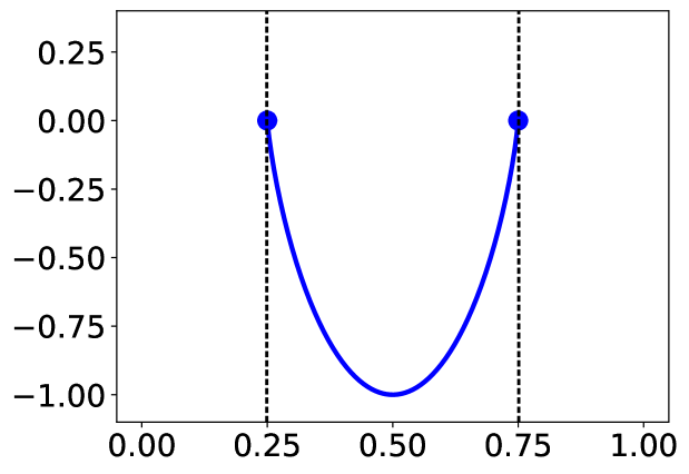
(b) $[0.25,0.75]$; no.

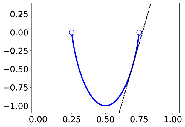
(c) $(0.25,0.75)$; yes.

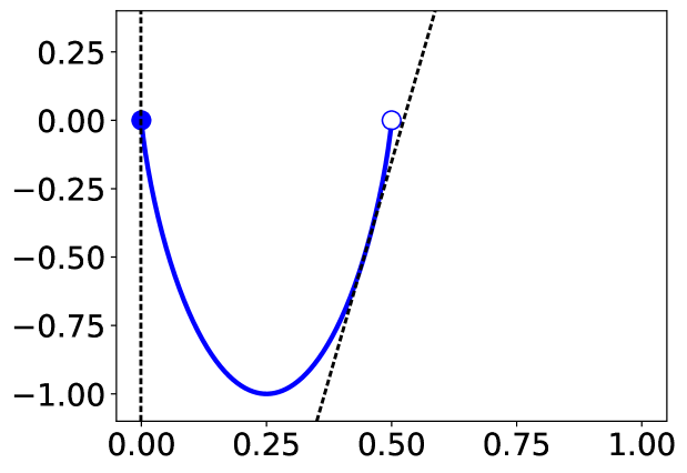
(d) $[0.0,0.5)$; yes.

The following definition will capture extended subgradients that lead to regular scoring rules. Recall from Proposition 2.6 that a linear extended function has a unique parameterization in Algorithm 1. Because we may have $t=0$ and $\textrm{Supp}\mathopen{}\mathclose{{}\left(p}\right)=\mathcal{Y}$, the conditions can be vacuously true.

Definition 4.11 (Interior-finite).

Say a linear extended function $f:\mathbb{R}^{\mathcal{Y}}\to\overline{\mathbb{R}}$ is $p$-interior-finite for $p\in\Delta_{\mathcal{Y}}$ if its parameterization in Algorithm 1 has: (1) for all pairs $y,y^{\prime}\in\textrm{Supp}\mathopen{}\mathclose{{}\left(p}\right)$, that $v_{j}(y)=v_{j}(y^{\prime})$ for all $j=1,\dots,t$; and (2) for all $y\not\in\textrm{Supp}\mathopen{}\mathclose{{}\left(p}\right)$ and $y^{\prime}\in\textrm{Supp}\mathopen{}\mathclose{{}\left(p}\right)$, that $v_{j}(y)=v_{j}(y^{\prime})$ for some sequence $j=1,\dots,k$, with either $k=t$ or else $v_{k+1}(y)<v_{k+1}(y^{\prime})$.

If $f$ is $p$-interior-finite, then property (1) gives that $f(q-p)$ is finite for $q$ in the face of the simplex generated by the support of $p$. (2) gives that $f(q-p)$ is either finite or $-\infty$ at all $q\in\Delta_{\mathcal{Y}}$ that are not in that face. These are the key properties that we will need for regular scoring rules.

Lemma 4.12 (Interior-finite implies quasi-integrable).

Let $p\in\Delta_{\mathcal{Y}}$. A linear extended function $f:\mathbb{R}^{\mathcal{Y}}\to\overline{\mathbb{R}}$ is $p$-interior-finite if and only if $f(\delta_{y}-p)\in\mathbb{R}\cup\{-\infty\}$ for all $y\in\mathcal{Y}$. Furthermore, in this case $f(\delta_{y}-p)\in\mathbb{R}$ for any $y\in\textrm{Supp}\mathopen{}\mathclose{{}\left(p}\right)$.

Proof.

Let $f$ be a linear extended function and $v_{1},\dots,v_{t}$ its unit vectors in the parameterization of Algorithm 1.

$(\implies)$ Suppose $f$ is $p$-interior-finite. If it is finite everywhere, then the conclusion is immediate. Otherwise, let $y\in\textrm{Supp}\mathopen{}\mathclose{{}\left(p}\right)$. Using that $v_{1}(y)=v_{1}(y^{\prime})$ for any $y^{\prime}\in\textrm{Supp}\mathopen{}\mathclose{{}\left(p}\right)$, we have

$$v_{1}\cdot(\delta_{y}-p) =v_{1}(y)-v_{1}\cdot p$$

$$=v_{1}(y)-\sum_{y^{\prime}\in\textrm{Supp}\mathopen{}\mathclose{{}\left(p}\right)}v_{1}(y^{\prime})p(y^{\prime})$$

$$=v_{1}(y)-v_{1}(y)\sum_{y^{\prime}\in\textrm{Supp}\mathopen{}\mathclose{{}\left(p}\right)}p(y^{\prime})$$

$$=0.$$

This applies to each successive $v_{j}$, so $f(\delta_{y}-p)\in\mathbb{R}$.

Now let $y\not\in\textrm{Supp}\mathopen{}\mathclose{{}\left(p}\right)$. Having just shown $v_{1}\cdot(\delta_{y^{\prime}}-p)=0$ for any $y^{\prime}\in\textrm{Supp}\mathopen{}\mathclose{{}\left(p}\right)$, we have $v_{1}\cdot(\delta_{y}-p)=v_{1}\cdot(\delta_{y}-\delta_{y^{\prime}})=v_{1}(y)-v_{1}(y^{\prime})\leq 0$ by assumption of $p$-interior-finite. So either Algorithm 1 returns $-\infty$ in the first iteration, or we continue to the second iteration. The same argument applies at each iteration, so $f(\delta_{y}-p)\in\mathbb{R}\cup\{-\infty\}$.

$(\impliedby)$ Suppose $f(\delta_{y}-p)\in\mathbb{R}\cup\{-\infty\}$ for all $y\in\mathcal{Y}$. Again if $f$ is finite everywhere, it is $p$-interior-finite, QED. So suppose its depth is at least $1$. We must have $v_{1}\cdot(\delta_{y}-p)\leq 0$ for all $y\in\mathcal{Y}$. This rearranges to $v_{1}(y)\leq v_{1}\cdot p$ for all $y$, or $\max_{y\in\mathcal{Y}}v_{1}(y)\leq v_{1}\cdot p$. But $p$ is a probability distribution, so $v_{1}\cdot p\leq\max_{y\in\mathcal{Y}}v_{1}(y)$. So $v_{1}\cdot p=\max_{y\in\mathcal{Y}}v_{1}(y)$. This implies that $v_{1}(y)=v_{1}(y^{\prime})=v_{1}\cdot p$ for all $y,y^{\prime}\in\textrm{Supp}\mathopen{}\mathclose{{}\left(p}\right)$. So $v_{1}\cdot(\delta_{y}-p)=0$ if $y\in\textrm{Supp}\mathopen{}\mathclose{{}\left(p}\right)$. Meanwhile, if $y\not\in\textrm{Supp}\mathopen{}\mathclose{{}\left(p}\right)$, then $v_{1}(y)\leq v_{1}\cdot p=v_{1}(y^{\prime})$ for any $y^{\prime}\in\textrm{Supp}\mathopen{}\mathclose{{}\left(p}\right)$.

This argument repeats to prove that if $y\in\textrm{Supp}\mathopen{}\mathclose{{}\left(p}\right)$, then for all $j=1,\dots,t$, $v_{j}(y)=\max_{y^{\prime}\in\mathcal{Y}}v_{j}(y^{\prime})$ and also $v_{j}\cdot(\delta_{y}-p)=0$. So it also gives $f(\delta_{y}-p)\in\mathbb{R}$. Meanwhile, if $y\not\in\textrm{Supp}\mathopen{}\mathclose{{}\left(p}\right)$, then we have a sequence $v_{1}(y)=\max_{y^{\prime}\in\mathcal{Y}}v_{1}(y^{\prime})$, …, $v_{k}(y)=\max_{y^{\prime}\in\mathcal{Y}}v_{k}(y^{\prime})$, where in each case $v_{j}\cdot(\delta_{y}-p)=0$. Then finally, either $k=t$ and $f(\delta_{y}-p)\in\mathbb{R}$, or we have $v_{k+1}(y)<\max_{y^{\prime}\in\mathcal{Y}}v_{k+1}(y^{\prime})$ and $f(\delta_{y}-p)=-\infty$. ∎

We can now make the key definition for the scoring rule characterization.

Definition 4.13 (Interior-locally-Lipschitz).

For $\mathcal{P}\subseteq\Delta_{\mathcal{Y}}\cap\textrm{effdom}\mathopen{}\mathclose{{}\left(g}\right)$, say $g:\mathbb{R}^{d}\to\mathbb{R}\cup\{\infty\}$ is $\mathcal{P}$-interior-locally-Lipschitz if $g$ has at every $p\in\mathcal{P}$ a $p$-interior-finite extended subgradient.

An interior-locally-Lipschitz $g$ simply has two conditions on its vertical supporting hyperplanes. First, they cannot cut faces of the simplex whose relative interior intersects $\textrm{effdom}\mathopen{}\mathclose{{}\left(g}\right)$; they can only contain them. This is enforced by $v_{j}(y)=v_{j}(y^{\prime})$ for $y,y^{\prime}\in\textrm{Supp}\mathopen{}\mathclose{{}\left(p}\right)$. In other words, the extended subgradients must be finite (in particular bounded, an analogy of causing $g$ to be Lipschitz) relative to the affine hull of these faces. Second, they must be oriented correctly so as not to cut that face from the rest of the simplex. This is enforced by $v_{j}(y)\leq v_{j}(y^{\prime})$ for $y\not\in\textrm{Supp}\mathopen{}\mathclose{{}\left(p}\right)$, $y^{\prime}\in\textrm{Supp}\mathopen{}\mathclose{{}\left(p}\right)$.

Lemma 4.12 gives the following corollary, in which the word “regular” is the point:

Corollary 4.14.

A convex $g:\mathbb{R}^{\mathcal{Y}}\to\mathbb{R}\cup\{\infty\}$ with $\textrm{effdom}\mathopen{}\mathclose{{}\left(g}\right)\supseteq\mathcal{P}$ has a regular subtangent scoring rule if and only if it is $\mathcal{P}$-interior-locally-Lipschitz.

Proof.

$(\implies)$ Suppose $g$ has a regular subtangent scoring rule $S(p,y)=g(p)+f_{p}(\delta_{y}-p)$, where $f_{p}$ is an extended subgradient of $g$ at $p$. By regularity, $f_{p}(\delta_{y}-p)\in\mathbb{R}\cup\{-\infty\}$, so by Lemma 4.12, $f_{p}$ is $p$-interior-finite. So $g$ has a $p$-interior-finite subgradient at every $p\in\mathcal{P}$, so it is $\mathcal{P}$-interior-locally-Lipschitz.

$(\impliedby)$ Suppose $g$ is $\mathcal{P}$-interior-locally-Lipschitz; then it has at each $p\in\mathcal{P}$ a $p$-interior-finite subgradient $f_{p}$. Let $S(p,y)=g(p)+f_{p}(\delta_{y}-p)$; by definition of $p$-interior-finite, $f_{p}(\delta_{y}-p)$ is never $+\infty$, so $S$ is regular, and it is a subtangent score. ∎

Theorem 4.15 (Construction of scoring rules on $\mathcal{P}$).

Let $\mathcal{Y}$ be a finite set and $\mathcal{P}\subseteq\Delta_{\mathcal{Y}}$.

1. Let $g:\mathbb{R}^{\mathcal{Y}}\to\mathbb{R}\cup\{\infty\}$ be convex and $\mathcal{P}$-interior-locally-Lipschitz with $\textrm{effdom}\mathopen{}\mathclose{{}\left(g}\right)\supseteq\mathcal{P}$. Then: (a) $g$ has at least one subtangent scoring rule that is regular; and (b) all of its subtangent scoring rules that are regular are proper; and (c) if $g$ is strictly convex on $\mathcal{P}$, then all of its regular subtangent rules are strictly proper.

2. Let $S:\mathcal{P}\times\mathcal{Y}\to\mathbb{R}\cup\{-\infty\}$ be a regular proper scoring rule. Then: (a) it is a subtangent rule of some convex $\mathcal{P}$-interior-locally-Lipschitz $g:\mathbb{R}^{\mathcal{Y}}\to\mathbb{R}\cup\{\infty\}$ with $\textrm{effdom}\mathopen{}\mathclose{{}\left(g}\right)\supseteq\mathcal{P}$; and (b) if $S$ is strictly proper and $\mathcal{P}$ a convex set, then any such $g$ is strictly convex on $\mathcal{P}$.

Observe that in (1), $g$ may have some subtangent rules that are regular and some that are not, depending on the choices of extended subgradients at each $p$. (1) only claims that there exists at least one choice that is regular (and therefore proper). An example is if $\mathcal{P}=\textrm{effdom}\mathopen{}\mathclose{{}\left(g}\right)$ is a single point, say the uniform distribution; vertical tangent planes will not work, but finite subgradients will. (This issue did not arise in the previous section where $\mathcal{P}=\Delta_{\mathcal{Y}}$; there, all of a convex $g$’s subtangent rules were regular.)

Proof.

(1) Let such a $g$ be given. We first prove that there exists a regular subtangent scoring rule of $g$. At each $p\in\mathcal{P}$, let $f_{p}$ be a $p$-interior-finite extended subgradient of $g$, guaranteed by definition of interior-locally-Lipschitz. Let $S:\mathcal{P}\times\mathcal{Y}\to\overline{\mathbb{R}}$ be of the form $S(p,y)=g(p)+f_{p}(\delta_{y}-p)$. Applying Lemma 4.12, $f_{p}(\delta_{y}-p)\in\mathbb{R}\cup\{-\infty\}$, so $S(p,y)\neq\infty$, so it is a regular scoring rule, proving (a).

Now, let $S$ be any regular subtangent scoring rule of $g$; we show $S$ is proper. Immediately we have an affine expected score function at each $p$ satisfying $S_{p}(q)=g(p)+f_{p}(q-p)$ for all $p\in\mathcal{P}$ and all $q\in\Delta_{\mathcal{Y}}$. We have $S_{p}(p)\geq S_{q}(p)$ for all $q$ because $S_{p}$ supports $g$ at $p$, so $S$ is proper, proving (b). Furthermore, if $g$ is strictly convex, then each $S_{q}$ supports $g$ at just one point in its effective domain (Lemma 3.11). So $S_{p}(p)>S_{q}(p)$ for $p,q\in\mathcal{P}$ with $q\neq p$, so $S$ is strictly proper, proving (c).

(2) Let a regular proper scoring rule $S$ be given. It has by Lemma 4.8 an affine extended expected score function $S_{p}$ at each $p\in\mathcal{P}$. Define $g:\mathbb{R}^{\mathcal{Y}}\to\mathbb{R}\cup\{\infty\}$ by $g(q)=\sup_{p\in\mathcal{P}}S_{p}(q)$. This is convex by Proposition 3.7. By definition of proper, for all $p\in\mathcal{P}$, we have $S_{p}(p)=\max_{q\in\mathcal{P}}S_{q}(p)=g(p)$. So $S_{p}$ is an affine extended function supporting $g$ at $p$, so it can be written $S_{p}(q)=g(p)+f_{p}(q-p)$ for some subgradient $f_{p}$ of $g$ at $p$. By definition of extended expected score, $S(p,y)=S_{p}(\delta_{y})=g(p)+f_{p}(\delta_{y}-p)$, so it is a subtangent rule.

Next, since $S$ is a scoring rule, in particular $S_{p}(\delta_{y})\in\mathbb{R}\cup\{-\infty\}$ for all $y$. So by Lemma 4.12, each $f_{p}$ is $p$-interior-finite, so $g$ is interior-locally-Lipschitz, proving (a).

Now suppose $S$ is strictly proper and $\mathcal{P}$ a convex set. Then for any $q\in\mathcal{P}$, we have that $S_{q}$ supports $g$ at $q$ alone out of all points in $\mathcal{P}$, by definition of strict properness. By Lemma 3.11, $g$ is strictly convex on $\mathcal{P}$, proving (b). ∎

There remain open directions investigating interior-locally-Lipschitz functions. Two important cases can be immediately resolved:

• If $\mathcal{P}\subseteq\textrm{int}\mathopen{}\mathclose{{}\left(\Delta_{\mathcal{Y}}}\right)$, then $g$ is $\mathcal{P}$-interior-locally-Lipschitz if $g$ is subdifferentiable on $\mathcal{P}$, i.e. has finite subgradients everywhere on $\mathcal{P}$. This follows because every $p\in\mathcal{P}$ has full support. More rigorously, this must be true of $g$ when restricted to the affine hull of the simplex; its subgradients can still be infinite perpendicular to the simplex, e.g. of the form $f(x)=\infty\cdot(x\cdot\vec{1})+\hat{f}(x)$.

• If $\mathcal{P}$ is an open set relative to the affine hull of $\Delta_{\mathcal{Y}}$, then every convex function $g$ with $\textrm{effdom}\mathopen{}\mathclose{{}\left(g}\right)\supseteq\mathcal{P}$ is $\mathcal{P}$-interior-locally-Lipschitz. This follows from the previous case along with the fact that convex functions are subdifferentiable on open sets in their domain.

One question for future work is whether one can optimize efficiently over the space of interior-locally-Lipschitz $g$, for a given set $\mathcal{P}\subseteq\Delta_{\mathcal{Y}}$. This could be useful in constructing proper scoring rules that optimize some objective.

Finally, we restate the general-$\mathcal{P}$ construction using the notation of Remark 4.10.

Remark 4.16.

Let $\mathcal{L}(\mathcal{P})$ be the set of $\mathcal{P}$-interior-locally-Lipschitz convex $g$ with effective domain containing $\mathcal{P}$, with $\mathcal{L}^{+}(\mathcal{P})$ those that are strictly convex on $\mathcal{P}$ and $\mathcal{L}^{-}(\mathcal{P})$ those that are not.

The characterization (prior work) states $\textrm{Reg}(\mathcal{P})\cap\textrm{Proper}(\mathcal{P})=\textrm{Reg}(\mathcal{P})\cap\textrm{ST}(\mathcal{C}(\mathcal{P}))$; the construction (Theorem 4.15) states $\textrm{Proper}(\mathcal{P})=\textrm{Reg}(\mathcal{P})\cap\textrm{ST}(\mathcal{L}(\mathcal{P}))$. In other words, if a subtangent rule of $g$ is regular, then $g$ is $\mathcal{P}$-interior-locally-Lipschitz. Similarly, the characterization states $\textrm{Reg}(\mathcal{P})\cap\textrm{StrictProper}(\mathcal{P})=\textrm{Reg}(\mathcal{P})\cap\textrm{ST}(\mathcal{C}^{+}(\mathcal{P}))$, while Theorem 4.15 states $\textrm{StrictProper}(\mathcal{P})=\textrm{Reg}(\mathcal{P})\cap\textrm{ST}(\mathcal{L}^{+}(\mathcal{P}))$.

Theorem 4.15 furthermore states that $\textrm{Reg}(\mathcal{P})\cap\textrm{ST}(\mathcal{L}^{-}(\mathcal{P}))\cap\textrm{ST}(\mathcal{L}^{+}(\mathcal{P}))=\emptyset$, i.e. strict properness exactly corresponds to strict convexity. Finally, it also states that for any particular $g$, $\textrm{Reg}(\mathcal{P})\cap\textrm{ST}(g)\neq\emptyset$ if and only if $g\in\mathcal{L}(\mathcal{P})$, i.e. $g$ has a regular subtangent rule if and only if it is convex and $\mathcal{P}$-interior-locally-Lipschitz.

References

- Chen and Waggoner [2016] Yiling Chen and Bo Waggoner. Informational substitutes. In 56th Annual IEEE Symposium on Foundations of Computer Science, FOCS ’16, 2016.
- Frongillo and Kash [2014] Rafael Frongillo and Ian Kash. General truthfulness characterizations via convex analysis. In Proceedings of the 10th Conference on Web and Internet Economics, WINE ’14, pages 354–370. Springer, 2014.
- Gneiting and Raftery [2007] Tilman Gneiting and Adrian E. Raftery. Strictly proper scoring rules, prediction, and estimation. Journal of the American Statistical Association, 102(477):359–378, 2007.
- Good [1952] Irving J. Good. Rational decisions. Journal of the Royal Statistical Society, 14(1):107–114, 1952.
- Hendrickson and Buehler [1971] Arlo D. Hendrickson and Robert J. Buehler. Proper scores for probability forecasters. The Annals of Mathematical Statistics, 42(6):1916–1921, 12 1971.
- Hiriart-Urrut and Lemaréchal [2001] Jean-Baptiste Hiriart-Urrut and Claude Lemaréchal. Fundamentals of Convex Analysis. Springer, 2001.
- Marschak [1959] Jacob Marschak. Remarks on the Economics of Information, pages 91–117. Springer Netherlands, 1959. ISBN 978-94-010-9278-4.
- McCarthy [1956] John McCarthy. Measures of the value of information. Proceedings of the National Academy of Sciences, 42(9):654–655, 1956.
- Rockafellar [1970] R. Tyrrell Rockafellar. Convex analysis. Princeton University Press, 1970.
- Savage [1971] Leonard J. Savage. Elicitation of personal probabilities and expectations. Journal of the American Statistical Association, 66(336):783–801, 1971.
- Schervish [1989] Mark J. Schervish. A general method for comparing probability assessors. The Annals of Statistics, 17(4):1856–1879, 12 1989. doi: 10.1214/aos/1176347398. URL https://doi.org/10.1214/aos/1176347398.