Vibrational CARS measurements in a near-atmospheric pressure plasma jet in nitrogen: II. Analysis

Abstract

The understanding of the ro-vibrational dynamics in molecular (near)-atmospheric pressure plasmas is essential to investigate the influence of vibrational excited molecules on the discharge properties. In a companion paper [1], results of ro-vibrational coherent anti-Stokes Raman scattering (CARS) measurements for a nanosecond pulsed plasma jet consisting of two conducting molybdenum electrodes with a gap of $1\text{\,}\mathrm{m}\mathrm{m}$ in nitrogen at $200\text{\,}\mathrm{m}\mathrm{b}\mathrm{a}\mathrm{r}$ are presented. Here, those results are discussed and compared to theoretical predictions based on rate coefficients for the relevant processes found in the literature. It is found, that during the discharge the measured vibrational excitation agrees well with predictions obtained from the rates for resonant electron collisions calculated by Laporta et al[2]. The predictions are based on the electric field during the discharge, measured by EFISH [1, 3] and the electron density which is deduced from the field and mobility data calculated with Bolsig+ [4]. In the afterglow a simple kinetic simulation for the vibrational subsystem of nitrogen is performed and it is found, that the populations of vibrational excited states develop according to vibrational-vibrational transfer on timescales of a few $\mathrm{\SIUnitSymbolMicro s}$, while the development on timescales of some hundred $\mathrm{\SIUnitSymbolMicro s}$ is determined by the losses at the walls. No significant influence of electronically excited states on the populations of the vibrational states visible in the CARS measurements ($v\lesssim 7$) was observed.

1 Introduction

In recent years, (near-) atmospheric pressure plasmas have gained a lot of interest in the plasma community due to their numerous possible applications. Those plasmas often employ relatively complex gas mixtures including molecular gases. Depending on the discharge conditions a significant amount of the energy input can be stored in the vibrational excitation of molecules, which can potentially enhance chemical reactions leading to possible use cases in plasma chemistry [5] and plasma catalysis [6, 7]. To investigate the influence of the vibrational excitation it is critical to know the vibrational distribution function. Besides tunable diode laser absorption spectroscopy (TDLAS), Fourier transform infrared (FTIR) spectroscopy and spontaneous Raman scattering, coherent anti-Stokes Raman scattering (CARS) is a popular technique to measure the vibrational excitation in gaseous media which was already employed in plasmas in the past [8]. Nonetheless, CARS has a drawback in the sense that the measured signal does depend on the population differences between vibrational states, i.e. the populations cannot be determined directly from the measured CARS spectra. This is not a major problem only for equilibrium systems where the vibrational population densities follow a Boltzmann distribution. With the knowledge of the distribution function theoretical CARS spectra can be calculated and fitted to measured ones with the temperature as fitting parameter [9]. The use of a simple Boltzmann distribution function is not possible in non-equilibrium systems as low-temperature plasmas. Here, several different evaluation methods were used in the past. One approach is to estimate the population density of one state and use this as starting point to calculate the others with the population differences obtained from the CARS spectra. This is done for example in an early work related to CARS in plasmas by Shaub et al[10] where the densities of the first two vibrational states were estimated by assuming a Boltzmann distribution for those. In other works[11, 12] it is assumed that the upper state for the highest detectable transition is approximately zero. The latter approximation is certainly reasonable for vibrational temperatures close to room temperature where the ratio between two neighboring states is about $\frac{N_{v+1}}{N_{v}}\approx\exp\left(-\frac{\hbar\omega_{e}}{k_{B}T_{vib}}\right)\approx 1.2\times 10^{-5}$ with $\omega_{e}\approx$2359\text{\,}\mathrm{c}\mathrm{m}^{-1}$$ and $T_{vib}=$300\text{\,}\mathrm{K}$$. This changes drastically for higher temperatures, e.g. $T_{vib}=$5000\text{\,}\mathrm{K}$$ where $\frac{N_{v+1}}{N_{v}}\approx 0.5$. For this reason in our companion paper [1] a different approach is used. Similar to CARS measurements in thermal equilibrium a distribution function is assumed for fitting theoretical spectra to measured ones, like it was done already by Messina et al[13] in a plasma burner. They assume that both the vibrational and the rotational decree of freedom are Boltzmann distributed, but have different temperatures. This works reasonably well for their measurements as they measure only up to the third vibrational state to the limited spectral range. In our measurements in [1] and previous CARS measurements in different plasma sources it can be seen that usually the higher vibrational states are overpopulated compared to a Boltzmann distribution determined by the first two or three vibrational states. For this reason a distribution function is chosen which includes two vibrational temperatures and one rotational, either called vibrational two-temperature distribution or simply two-temperature distribution function (TTDF) in the following. As the TTDF is motivated by the underlying plasma physics in the discharge, a detailed derivation was omitted in [1] where the focus was on the diagnostic method. In the present paper we motivate the use of the TTDF based on the excitation processes in the plasma in section 3.1. Additionally, simple models are derived for the parameters in the TTDF connecting them to the plasma parameters. Finally, the population difference results from [1] in the afterglow where the TTDF is not valid anymore are compared to a simple kinetic model for the vibrational subsystem in section 3.2.

2 Summary of the results in [1]

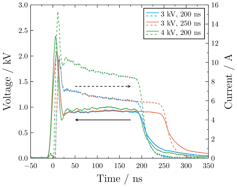
Figure 1: Voltages (solid) and currents (dashed) at the cathode used for the measurements in [1].

In [1] a ns-pulsed discharge with a parallel electrode configuration is studied. The discharge jet consists of two molybdenum electrodes with a length of $20\text{\,}\mathrm{m}\mathrm{m}$ and a thickness of $1\text{\,}\mathrm{m}\mathrm{m}$. The $1\text{\,}\mathrm{m}\mathrm{m}$ gap between the electrodes is enclosed with two glass plates at the long edges of the electrodes. In the middle of one glass plate a hole with about $1\text{\,}\mathrm{m}\mathrm{m}$ diameter serves as gas inlet. This way two opposing gas channels with a $$1\text{\,}\mathrm{m}\mathrm{m}$\times$1\text{\,}\mathrm{m}\mathrm{m}$$ cross section and $10\text{\,}\mathrm{m}\mathrm{m}$ length are constructed. By applying a high voltage to one of the electrodes while grounding the other an electric field can be created transverse to the gas flow. This geometry was chosen to provide a simple model geometry for nanosecond pulsed discharges in a pressure range close to atmospheric pressure (about $100\text{\,}\mathrm{m}\mathrm{b}\mathrm{a}\mathrm{r}$ up to $1\text{\,}\mathrm{b}\mathrm{a}\mathrm{r}$). It should be noted that in contrast to the dielectric barrier discharges (DBD) more often used to operate nanosecond pulsed plasmas around atmospheric pressure, here a conduction current can flow for as long as several hundred nanoseconds depending on the power supply. This was seen to have major impact on the vibrational excitation in [1].
The discharge is operated in pure nitrogen at a pressure of $200\text{\,}\mathrm{m}\mathrm{b}\mathrm{a}\mathrm{r}$ and a gas flow of $20\text{\,}\mathrm{s}\mathrm{c}\mathrm{c}\mathrm{m}$. A high voltage pulse is applied with $200\text{\,}\mathrm{n}\mathrm{s}$ or $250\text{\,}\mathrm{n}\mathrm{s}$ pulse length (see figure 1) and a repetition rate of $1\text{\,}\mathrm{k}\mathrm{H}\mathrm{z}$. The applied voltages lead to the current waveforms depicted in figure 1 with a high current peak during the ignition of the discharge and a relatively constant, lower current plateau for the remainder of the discharge pulse due to a voltage drop at a series resistor. These condition produce a homogeneous discharge along the gas channel without arcing. The electric field is measured in the middle of the discharge at multiple times during the constant current plateau via the E-FISH technique and measurements of the ro-vibrational distributions are performed by coherent anti-Stokes Raman scattering (CARS) during the discharge pulse and in the afterglow between two pulses for three different voltage pulses shown in figure 1. The electric field is found to be around $81\text{\,}\mathrm{T}\mathrm{d}$ at all times during the current plateau for all three discharge conditions. For the analysis of the measured CARS spectra a vibrational two-temperature distribution of the form

$$N(v,J;T_{rot},T_{vib,c},T_{vib,h},R_{h})=g(J)\mathrm{e}^{-\frac{E(v,J)-E(v,0)}{k_{B}T_{rot}}}$$ (1)

$$\times\Bigl{[}\frac{1-R_{h}}{Z_{c}}\mathrm{e}^{-\frac{E(v,0)-E(0,0)}{k_{B}T_{vib,c}}}+\underbrace{\frac{R_{h}}{Z_{h}}\mathrm{e}^{-\frac{E(v,0)-E(0,0)}{k_{B}T_{vib,h}}}}_{\text{for }v>0}\Bigr{]}$$

is proposed which distinguishes between the rotational(-translational) temperature $T_{rot}$ and two vibrational temperatures - $T_{vib,c}$ for a vibrationally cold distribution and $T_{vib,h}$ for a smaller, vibrationally hot distribution. For nitrogen the degeneracy of the rotational states is

$$g(J)=\left\{\begin{array}[]{@{\kern 2.5pt}lL}\hfill 6(2J+1),&\text{if } J \text{ even}\\ \hfill 3(2J+1),&\text{if } J \text{ odd.}\end{array}\right.$$ (2)

The partition function for the vib. cold molecules is given by

$$Z_{c}=\sum_{v,J}g(J)\mathrm{e}^{-\frac{E(v,J)-E(v,0)}{k_{B}T_{rot}}}\times\mathrm{e}^{-\frac{E(v,0)-E(0,0)}{k_{B}T_{vib,c}}}$$ (3)

and for the vib. hot molecules by

$$Z_{h}=\sum_{v>0,J}g(J)\mathrm{e}^{-\frac{E(v,J)-E(v,0)}{k_{B}T_{rot}}}\times\mathrm{e}^{-\frac{E(v,0)-E(0,0)}{k_{B}T_{vib,h}}}.$$ (4)

A detailed motivation of this distribution function is given in section 3.1 where also the measurement results are presented in figures 6 and 2 together with predictions from data for vibrational excitation by resonant electron collisions. It should be noted, that here and in the following particle densities are always normalized to one, i.e. they are divided by the gas density.
As (2) is motivated by the excitation processes in the discharge it is not adequate to describe the afterglow. Therefore, there only the population differences $\Delta N_{v}=N_{v}-N_{v+1}$ are inferred from the CARS spectra and the individual population densities are obtained by extrapolating the number density of the upper state of the highest detectable transition. For more details see [1]. Some results are shown in section 3.2 where they are compared with a simple volume averaged model for the vibrational system.

3 Description of the vibrational dynamics

3.1 Discharge phase

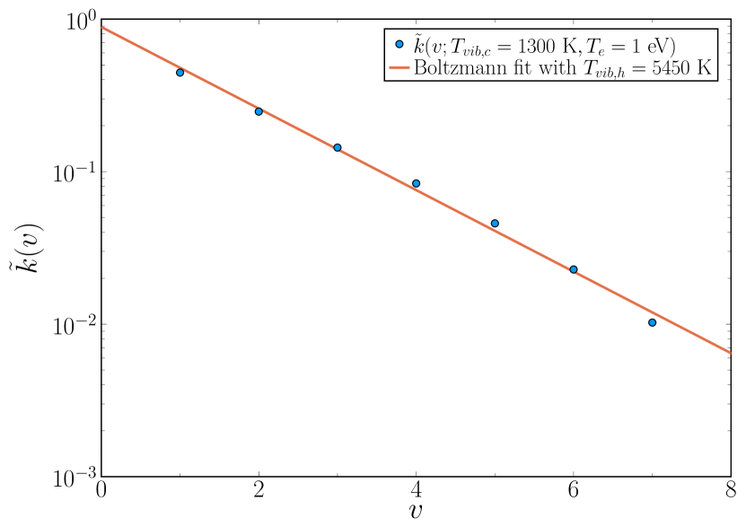
Figure 2: Sum of excitation rates into vibrational states $v$ for an electron temperature of $T_{e}=$1\text{\,}\mathrm{e}\mathrm{V}$$ and a vibrational background with a (vib.) temperature of $1300\text{\,}\mathrm{K}$ (normalized by $\sum_{v}\tilde{k}(v)$). The solid line is a Boltzmann distribution with a temperature of $5450\text{\,}\mathrm{K}$.

Figure 3: Temperature of the newly excited states in dependence of electron and vibrational temperature before the discharge.

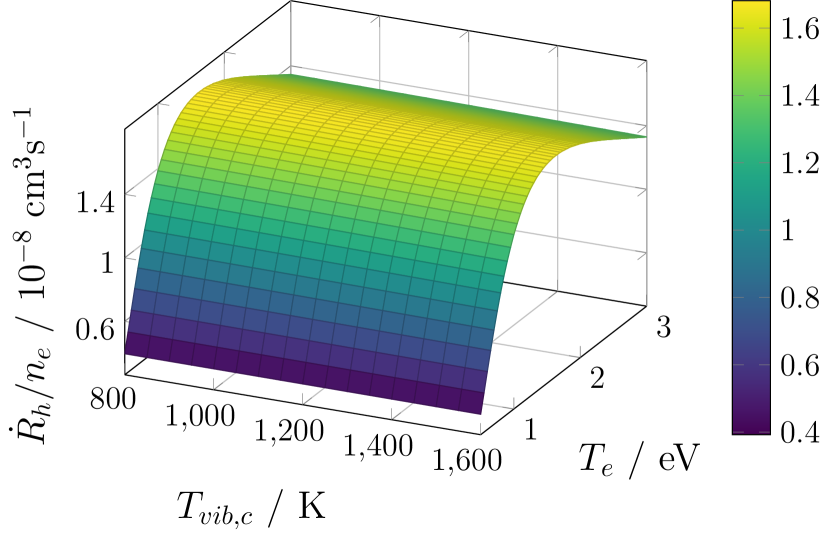
Figure 4: Dependence of $R_{h}/n_{e}$ on the temperature of the cold molecules and the electrons.

The two-temperature distribution function in equation 2 was already introduced in [1] but not further motivated. This shall be done here.
The main concept of equation 2 is that the nitrogen molecules can be divided into two mostly independent populations

$$N(v,J)=$$ (5)

$$N_{c}(v,J;T_{rot},T_{vib,c},R_{h})+N_{h}(v,J;T_{rot},T_{vib,h},R_{h})$$

where the population of the vibrationally cold molecules is characterized by the cold temperature $T_{vib,c}$ and the population of the hot molecules by the hot temperature $T_{vib,h}$. Both populations share the same rotational temperature $T_{rot}$ and the fraction of hot and cold molecules compared to the total amount of nitrogen is given by $R_{h}$ and $(1-R_{h})$ respectively.
On time scales of the nanosecond pulse there is essentially no exchange of vibrational excitation among the nitrogen molecules as V-V and V-T collisions are important only on longer time scales. The dominant process of vibrational excitation during the discharge is most certainly excitation by resonant electron collisions [5]. This leads to the following interpretation of the two distributions: $N_{c}$ is the steady-state background distribution which comprises the bulk of the nitrogen molecules. During the discharge some molecules are transferred from $N_{c}$ to $N_{h}$ by electron collisions. This means the total excitation rate $\dot{R_{h}}$ and the vibrational temperature of the newly excited molecules are solely defined by the corresponding cross sections, the electron density and the electron temperature.
For the analysis of the measurements in [1] the cross section and rate dataset calculated by Laporta et al [14, 15, 2] - freely accessible in the Phys4Entry database [16] - is used. First the characteristics of the hot distribution are investigated. While in (2) a Boltzmann distribution is assumed, there is no obvious physical reason which suggests this choice. To see that the Boltzmann distribution is still a reasonable good approximation for the range of vibrational states visible in this work in the following the excitation process is investigated. To begin we assume, that the electron conditions during most of the discharge are essentially constant. This is motivated by the constant electric field in [1] and the nearly constant current. So the rate equation for a vibrational state $v\geq 1$ is given by

$$\dot{N}_{v}=\sum_{i<v}N_{i}k(i,v;T_{e})n_{e},$$ (6)

where $n_{e}$ is the electron density and $k(i,v;T_{e})$ is the rate coefficient for the resonant excitation by electron collisions from vibrational state $i$ to $v$ at the electron temperature $T_{e}$. Here, the interest is only in the vibrational dynamics, so particle densities $N_{v}$ can be understood as integrated over the rotational quantum number. Now, we distinguish between the newly excited molecules (i.e. the ones which are excited during the current discharge pulse) $\tilde{N}_{v}$ and the bulk of the molecules $N_{i}$ which follows the cold distribution with temperature $T_{vib,c}$. For constant $n_{e}$ and $T_{e}$ the solution of equation 6 for $\tilde{N}_{v}$ with the initial condition $\tilde{N}_{v}(t=0)=0$ and under the assumption that the cold background stays constant, $N_{v}(t)=\mathrm{const}$, is trivial, and we find that

$$\tilde{N}_{v} =\left(\sum_{i<v}N_{i}k(i,v;T_{e})\right)n_{e}t$$

$$\propto\sum_{i<v}N_{i}(T_{vib,c})k(i,v;T_{e})=:\tilde{k}(v;T_{vib,c},T_{e}).$$

This means, that the shape of the distribution of the hot molecules is constant during the discharge and follows from the values of the corresponding rates. The sum of rates for all resonant electron processes into the vibrational states $v$ are depicted in figure 2 for an exemplary electron temperature of $T_{e}=$1\text{\,}\mathrm{e}\mathrm{V}$$ and a background temperature of $1300\text{\,}\mathrm{K}$. As can be seen the rates, and therefore populations of the excited states, follow a similar dependency on the vibrational quantum number $v$ as a Boltzmann distribution. This motivates the use of a Boltzmann distribution for the newly excited molecules. In this regard two points should be noted. First, the approximation with a Boltzmann distribution is not necessarily usable for conditions other than investigated in this work. For states $v>7$ in nitrogen significant deviations from a Boltzmann distribution are and also no statements are made for other gases here. Second, there is no explicit physical motivation behind the use of the Boltzmann distribution. Instead, it was chosen because the concept of temperatures is convenient and familiar. By more detailed examination of the resonant processes leading to vibrational excitation a more precise distribution might be found which is valid in regimes where this simple approximation fails. But for the purpose of this work a Boltzmann distribution is sufficient to describe the observed CARS spectra.
As presented in figure 2 the temperature of the hot molecules can be obtained by a fit to the rates from [2] for a given vibrational temperature of the molecule bulk and electron temperature. In figure 3 values for $T_{vib,h}$ calculated in this way are shown for a range of $T_{vib,c}$ and $T_{e}$. As can be seen the dependence on the vibrational bulk temperature is weak and decreases further for higher electron temperatures.

Figure 5: Temperature of the newly excited molecules as obtained by the CARS measurements [1]. For the measurement with $4\text{\,}\mathrm{k}\mathrm{V}$ and with $3\text{\,}\mathrm{k}\mathrm{V}$ applied voltage, the dark gray and the light gray shaded regions should not taken into account, respectively[1]. The solid line corresponds to the theoretical value for a vibrational bulk temperature of $1300\text{\,}\mathrm{K}$ and a electron temperature of $1.2\text{\,}\mathrm{e}\mathrm{V}$ (corresponding to a reduced electric field of $81\text{\,}\mathrm{T}\mathrm{d}$ according to BOLSIG+ calculations [4] with the IST Lisbon data set [17].)

For a comparison of the theoretical $T_{vib,h}$ the electron temperature is estimated with BOLSIG+ [4] and the IST Lisbon cross section data set [17] to be around $1.2\text{\,}\mathrm{e}\mathrm{V}$ for the measured reduced electric field of $81\text{\,}\mathrm{T}\mathrm{d}$. As the dependency on $T_{vib,c}$ is weak (see figure 3), in figure 5 the measurements are only compared to the theoretical value for $T_{vib,c}=$1300\text{\,}\mathrm{K}$$. Considering the drastic simplifications in the derivation of the theoretical value and the measurement uncertainty generally a good agreement can be observed.
In addition to the temperature of the newly excited molecules it is possible to estimate the rate of excitation. The parameter $R_{h}$ in (2) describes the total amount of newly excited molecules relative to the gas density. With (6) one obtains

$$\dot{R}_{h}=\frac{\partial}{\partial t}\left(\sum_{v>0}\tilde{N}_{v}\right)=\sum_{v>0}\tilde{k}(v;T_{vib,c},T_{e})n_{e}$$ (8)

for the derivative of $R_{h}$. In figure 4 the dependence of $\dot{R}_{h}/n_{e}$ is shown in a similar fashion as it is done for the temperature in figure 3, and it can be seen that there is essentially no dependence on the initial temperature for the excitation rate. Strictly speaking, (8) is only valid in the beginning of the discharge as it depends on the approximation $R_{h}\ll 1$. In our measurements we see an increase of $R_{h}$ up to about 0.1. Therefore, some minor correction need to be applied to (8). To account for the depletion of the cold background $N_{i}$ in (3.1) is multiplied by $(1-R_{h})$. Additionally, when $R_{h}$ increases the possibility of multiple vibrational excitation processes can become important. If molecules from $R_{h}$ are excited again and end up in states higher than the highest state visible in the CARS spectra, $v_{max}$, they cannot be seen in the measurement. Therefore, an effective loss rate $k_{loss}(v;R_{h},T_{vib,h},T_{e})$ is introduced. With these corrections (8) becomes

$$\dot{R}_{h}=\sum_{v>0} \Big{[}\tilde{k}^{\prime}(v,R_{h};T_{vib,c},T_{e})n_{e}$$

$$-k_{loss}(v,R_{h};T_{vib,h},T_{e})n_{e}\Big{]},$$

where $\tilde{k}^{\prime}$ and $k_{loss}$ can both be expressed analog to the definition of the TTDF (2) as

$$\tilde{k}^{\prime}(v,R_{h};T_{vib,c},T_{e})=\sum_{i<v}k(i,v;T_{e})\frac{1-R_{h}}{Z_{c}^{\prime}}\mathrm{e}^{-\frac{E(i,0)-E(0,0)}{k_{B}T_{vib,c}}}$$ (10)

and

$$k_{loss}(v,R_{h};T_{vib,h},T_{e})=\sum_{j>v_{max}}k(v,j;T_{e})\underbrace{\frac{R_{h}}{Z_{h}^{\prime}}\mathrm{e}^{-\frac{E(v,0)-E(0,0)}{k_{B}T_{vib,h}}}}_{\text{for }v>0}.$$ (11)

Here, the corresponding distributions are summed over the rotational quantum number which is reflected in the partition functions $Z_{c}^{\prime}$ and $Z_{h}^{\prime}$. Note, that because $T_{vib,h}(T_{vib,c},T_{e})$, (3.1) is not more complex than (8) in the sense, that it still depends only on the external parameters $n_{e}$, $T_{vib,c}$ and $T_{e}$.
As the electric field is constant during the current plateau the electron density can be calculated via

$$\frac{I(t)}{A}=\mu(E)En_{e}(t).$$ (12)

where $I(t)$ is the current measured in the plateau, $E$ the electric field obtained by the E-FISH measurements[1] and $A$ plasma cross section.

Figure 6: Fraction of the newly excited molecules during the discharge pulse. The solid lines are the theoretical rates calculated with the data from [2] for electron temperatures and densities obtained by current and field measurements for $4\text{\,}\mathrm{k}\mathrm{V}$ applied voltage (green) and $3\text{\,}\mathrm{k}\mathrm{V}$ (blue). The shaded ribbons give the uncertainty due to the uncertainty in the initial values.

Note, that during the high current pulse in the beginning the electric field can be much higher than in the plateau [3]. Therefore, (12) is only evaluated for $t>$20\text{\,}\mathrm{n}\mathrm{s}$$, i.e. during the plateau phase. In figure 6 $R_{h}$ calculated by integrating (3.1) is compared to the measured values of $R_{h}$ during the discharge pulse. The initial value for the integration is chosen to be the average of the three data points before the ignition of the discharge ($t<$0\text{\,}\mathrm{n}\mathrm{s}$$). A very good agreement is observed between the measurements and the theoretical values calculated from the current and field measurements even though those are completely independent of the CARS measurements.

3.2 Afterglow

To analyze the dynamics of vibrationally excited states in the afterglow between two discharge pulses a kinetic model is developed for vibrationally excited nitrogen up to $v=9$.
As the ionization degree is very low, superelastic collisions with the plasma electrons are neglected here. Furthermore, the influence of electronically excited molecules is ignored and the dissociation degree is assumed to be small. These assumptions reduce the reaction set to V-V and V-T collisions among the nitrogen molecules.
The rates for the V-V process

$$\textrm{N}_{2}(v+1)+\textrm{N}_{2}(w)\rightarrow\textrm{N}_{2}(v)+\textrm{N}_{2}(w+1)$$ (13)

are calculated from the rate for the process

$$\textrm{N}_{2}(1)+\textrm{N}_{2}(0)\rightarrow\textrm{N}_{2}(0)+\textrm{N}_{2}(1)$$ (14)

via the scaling law of the semiclassical forced harmonic oscillator (FHO) model[18, 19]

$$k_{VV}(v+1,w\rightarrow v,w+1)=$$ (15)

$$k_{VV}(1,0\rightarrow 0,1)(v+1)(w+1)\frac{3-\textrm{e}^{-\frac{2\lambda}{3}}}{2}\textrm{e}^{-\frac{2\lambda}{3}}\exp\left(\frac{\Delta E}{2k_{B}T}\right)$$

where $k_{B}$ is the Boltzmann constant and $T$ the gas temperature. $\lambda$ is given by [19]

$$\lambda=\frac{1}{3\sqrt{2}}\sqrt{\frac{\theta}{T}}\frac{|\Delta E|}{\omega\hbar}$$ (16)

with the harmonic angular frequency $\omega$ and $\theta=\frac{4\pi^{2}\omega^{2}m}{\alpha^{2}k_{B}}$. $\Delta E=E(v+1)+E(w)-E(v)-E(w+1)$ is the energy defect due to the anharmonicity of the vibrational potential, $m$ is the collisional reduced mass and $\alpha$ is the exponential repulsive potential parameter [19]. For $k_{VV}(1,0\rightarrow 0,1)$ the value $0.9\text{\times}{10}^{-14}\text{\,}{\mathrm{cm}}^{3}\text{\,}{\mathrm{s}}^{-1}$ is used [20].
For completeness the V-T rates from the calculations provided by Billing and Fisher [20] for a (rotational-translational) gas temperature of $300\text{\,}\mathrm{K}$ are included. It should be noted that they are several orders of magnitude smaller and do not affect the simulation in a noticeable way.
The simulation volume is one half of the discharge jet, i.e. a cuboid with edge lengths $$1\text{\,}\mathrm{m}\mathrm{m}$\times$1\text{\,}\mathrm{m}\mathrm{m}$\times$10\text{\,}\mathrm{m}\mathrm{m}$$. As first approximation the particle densities are assumed to be homogeneous in the whole volume. The influx of is considered via [21]

$$\left.\frac{dN_{0}}{dt}\right|_{in}=N_{gas}\frac{CQP_{atm}}{VP}$$ (17)

where $Q=$10\text{\,}\mathrm{s}\mathrm{c}\mathrm{c}\mathrm{m}$$ is half of the set gas flow - as it is assumed that the total gas flow of $20\text{\,}\mathrm{s}\mathrm{c}\mathrm{c}\mathrm{m}$ is split equally to both sides of the jet. $C=$1.6667\text{\times}{10}^{-8}\text{\,}\mathrm{{}^{3}}\mathrm{m}\mathrm{/}\mathrm{s}\mathrm{/}\mathrm{s}\mathrm{c}\mathrm{c}\mathrm{m}$$ is the conversion factor to convert $\mathrm{s}\mathrm{c}\mathrm{c}\mathrm{m}$ to ${\mathrm{m}}^{3}\text{\,}{\mathrm{s}}^{-1}$, $P_{atm}=$1\text{\,}\mathrm{b}\mathrm{a}\mathrm{r}$$ is the atmospheric pressure and $P=$200\text{\,}\mathrm{m}\mathrm{b}\mathrm{a}\mathrm{r}$$ is the pressure in the discharge chamber and $N_{gas}$ is the gas density. In (17) it is assumed, that the inflowing particles are all in the vibrational ground state as at room temperature there is now significant vibrational excitation. The vibrational excited nitrogen molecules in state $v$ exiting the jet are described by

$$\left.\frac{dN_{v}}{dt}\right|_{out}=-N_{v}\frac{CQP_{atm}}{VP}.$$ (18)

The loss of excited molecules by diffusion to the walls is given by [22, 21]

$$\left.\frac{\partial N_{v>0}}{\partial t}\right|_{W} =-N_{v>0}\left(\frac{\Lambda_{0}^{2}}{D_{v}}+\frac{2(2-\gamma_{v})V}{v_{th}\gamma_{v}A}\right)^{-1}$$

$$\approx-\frac{v_{th}\gamma_{v}A}{2(2-\gamma_{v})V}$$

with the characteristic length scale for the given geometry $\Lambda_{0}$ [22], the volume and surface area $V$ and $A$, the diffusion coefficient for the species $D_{v}$ and the corresponding deactivation coefficient $\gamma_{v}$ giving the probability to lose a particle in state $v$ when it hits the wall. $\gamma_{v}$ is not very well known for states $v>1$ but for $v=1$ it is typically in the order of about $4\text{\times}{10}^{-4}\text{\,}$ to $3\text{\times}{10}^{-3}\text{\,}$ for different materials [23]. In absence of better knowledge the deactivation coefficient is chosen here to be $\gamma=$1\text{\times}{10}^{-3}\text{\,}$$ for all states. This motivates the approximation in (3.2) which is consistent with the assumption of flat density profiles: the very low deactivation coefficient means that the loss of excited particles is not limited by the diffusion, but instead by the deactivation process once the molecules reach the walls. Finally, we assume that the deactivation happens directly into the ground state, so that the walls are effectively a source for $v=0$:

$$\left.\frac{\partial N_{0}}{\partial t}\right|_{W}=-\sum_{v>0}\left.\frac{\partial N_{v}}{\partial t}\right|_{W}$$ (20)

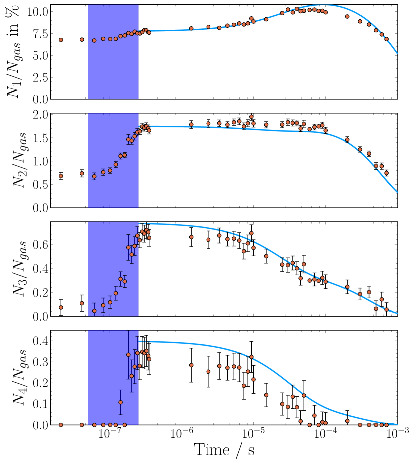
Figure 7: Relative population densities for the measurement $3\text{\,}\mathrm{k}\mathrm{V}$, $200\text{\,}\mathrm{n}\mathrm{s}$. Symbols are the population densities obtained with the method described in [1] and lines are the results from the kinetic model.

The initial conditions for the simulation are obtained from the two temperature distribution directly after the discharge pulse. In this way the initial population densities are extrapolated up to $v=9$. The results of the simulation are compared to the measurement results from [1] in figure 7. For clarity of presentation the results for the other two measurement conditions are shown in the appendix (see figures 8 and 9). Those show a similar good agreement.

From the very good agreement between the measurements and the simple simulation it can be inferred, that here the E-V transitions, i.e. population of vibrational states by deexcitation of electronically excited molecules, seem to play only a minor role in contrast to previous works [11, 12]. A possible reason to explain this difference could be a generally higher electric field in discharges therein, which increases the amount of electronic excitation. While there is not much information about the discharge used by Deviatov et al[11], Montello et al[12] used a pin-to-pin discharge with a $10\text{\,}\mathrm{m}\mathrm{m}$ gap. Their estimated electric field reaches up to about $275\text{\,}\mathrm{T}\mathrm{d}$ during the ignition phase and stays at about $125\text{\,}\mathrm{T}\mathrm{d}$ during the discharge plateau which is significantly higher than the value obtained by E-FISH measurements [1] in the discharge investigated here. Additionally, their pulse is only $150\text{\,}\mathrm{n}\mathrm{s}$ long which further increases the relative importance of the high electric field during the ignition. Therefore, it is very likely, that in their discharges the density of electronically excited states relative to the vibrationally excited states is significantly higher.

4 Conclusion

In this paper, the vibrational two-temperature distribution function used in the companion paper [1] to evaluate CARS spectra during a ns-pulsed discharge was motivated and the different parameters were connected to the underlying physical processes. It is found that under the investigated discharge conditions the direct resonant excitation through electron collisions is the main path for production of vibrationally excited nitrogen. The distribution function of the newly excited molecules follows therefore the shape of the corresponding excitation probabilities or rates. In the case of resonant excitation this shape closely resembles a Boltzmann distribution for small $v$, leading to the two-temperature distribution function (2) consisting of a Boltzmann distributed cold background and the also Boltzmann distributed newly excited hot molecules. For the case that the excitation rates do not follow a Boltzmann distribution the hot part of the distribution function can be modified easily. If sufficient data for the excitation process is known the parameter in the distribution function can be estimated, and it is found that the estimates - using the rates reported by Laporta [2] in combination with current and field measurements - agree very well with the measured values. This shows that the rather simple two-temperature distribution - and its generalization by allowing non-Boltzmann distributions - provides a useful framework for analyzing and potentially optimizing the vibrational excitation of molecules in plasmas where the resonant excitation by electron collisions is the dominant process. Furthermore, the fact that the current and electric field are nearly constant during almost the whole high voltage pulse for the discharge type investigated in this work, indicates a constant electron density during the majority of the discharge which is created essentially only during the ignition of the pulse. This promises an easy tool for estimating the amount of vibrational excitation a priori when one is able to predict the density and electric field for the given discharge.
For the afterglow it was found, that a relative simple model considering only V-V and V-T transfer and transport losses is enough to reproduce the measurements. Meaning E-V transfer - where vibrational excited molecules in the electronic ground state are produced by cascades or quenching of higher electronic states - seems to be of minor importance in this discharge type. A possible reason why E-V transfer was needed to explain previous vibrational measurements [11, 12] could be the generally higher electric field in those works.
Finally, it can be concluded that the discharge reactor investigated here shows promise to be a handy tool while investigating the influence of vibrational excitation for example on plasma chemistry or plasma catalysis. Together with the description of the vibrational system provided here it allows to easily control and understand the vibrational excitation in the plasma volume, which is vital to understand its influence on other reactions.

Appendix A Additional simulation results

For completeness here the results of the simulation are compared to the measurements ”$3\text{\,}\mathrm{k}\mathrm{V}$, $200\text{\,}\mathrm{n}\mathrm{s}$” and ”$4\text{\,}\mathrm{k}\mathrm{V}$, $200\text{\,}\mathrm{n}\mathrm{s}$” from [1] in figures 8 and 9. The agreement is as good as in figure 7, leading to the conclusion, that for all conditions investigated the processes included in the simulation are sufficient to explain the experimental results.

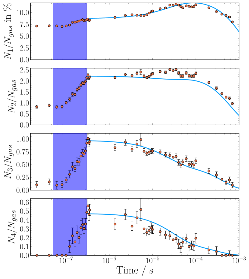
Figure 8: Relative population densities for the measurement $3\text{\,}\mathrm{k}\mathrm{V}$, $250\text{\,}\mathrm{n}\mathrm{s}$. Symbols are the population densities obtained with the method described in [1] and lines are the results from the kinetic model.

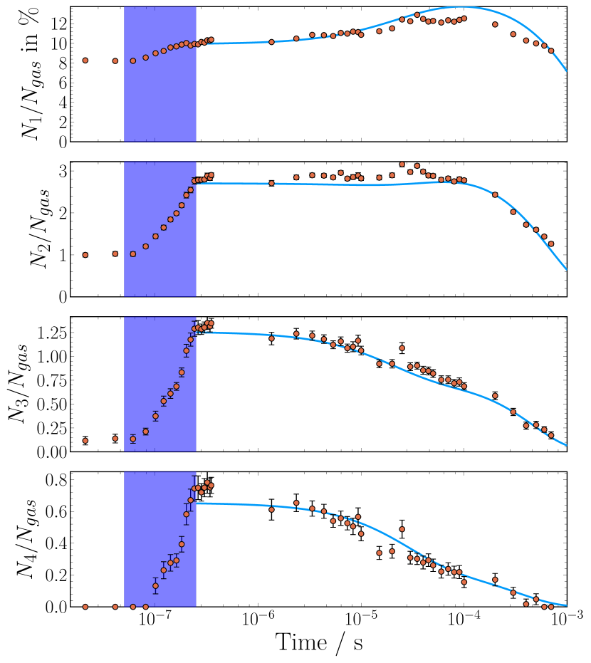
Figure 9: Relative population densities for the measurement $4\text{\,}\mathrm{k}\mathrm{V}$, $200\text{\,}\mathrm{n}\mathrm{s}$. Symbols are the population densities obtained with the method described in [1] and lines are the results from the kinetic model.

References

References

- [1] Kuhfeld J, Lepikhin N D, Luggenhölscher D and Czarnetzki U Vibrational CARS measurements in a near-atmospheric pressure plasma jet in nitrogen: I. Measurement procedure and results
- [2] Laporta V, Little D A, Celiberto R and Tennyson J 2014 Electron-impact resonant vibrational excitation and dissociation processes involving vibrationally excited N2 molecules Plasma Sources Science and Technology 23 065002
- [3] Lepikhin N D, Luggenhölscher D and Czarnetzki U 2020 Electric field measurements in a He:N2 nanosecond pulsed discharge with sub-ns time resolution Journal of Physics D: Applied Physics 54 055201
- [4] Hagelaar G J M and Pitchford L C 2005 Solving the Boltzmann equation to obtain electron transport coefficients and rate coefficients for fluid models Plasma Sources Science and Technology 14 722–733
- [5] Fridman A A 2008 Plasma chemistry first paperback edition ed (Cambridge: Cambridge University Press)
- [6] Neyts E C and Bogaerts A 2014 Understanding plasma catalysis through modelling and simulation—a review Journal of Physics D: Applied Physics 47 224010
- [7] Whitehead J C 2016 Plasma–catalysis: the known knowns, the known unknowns and the unknown unknowns Journal of Physics D: Applied Physics 49 243001
- [8] Lempert W R and Adamovich I V 2014 Coherent anti-Stokes Raman scattering and spontaneous Raman scattering diagnostics of nonequilibrium plasmas and flows Journal of Physics D: Applied Physics 47 433001
- [9] Eckbreth A C 1996 Laser diagnostics for combustion temperature and species 2nd ed (Combustion science and technology book series no volume 3) (Boca Raton: CRC Press)
- [10] Shaub W M, Nibler J W and Harvey A B 1977 Direct determination of non‐Boltzmann vibrational level populations in electric discharges by CARS The Journal of Chemical Physics 67 1883–1886
- [11] Deviatov A A, Dolenko S A, Rakhimov A T, Rakhimova T V and Roi N N 1986 Investigation of kinetic processes in molecular nitrogen by the CARS technique Zhurnal Eksperimentalnoi i Teoreticheskoi Fiziki 90 429–436
- [12] Montello A, Yin Z, Burnette D, Adamovich I V and Lempert W R 2013 Picosecond CARS measurements of nitrogen vibrational loading and rotational/translational temperature in non-equilibrium discharges Journal of Physics D: Applied Physics 46 464002
- [13] Messina D, Attal-Trétout B and Grisch F 2007 Study of a non-equilibrium pulsed nanosecond discharge at atmospheric pressure using coherent anti-Stokes Raman scattering Proceedings of the Combustion Institute 31 825–832
- [14] Laporta V, Celiberto R and Wadehra J M 2012 Theoretical vibrational-excitation cross sections and rate coefficients for electron-impact resonant collisions involving rovibrationally excited N2and NO molecules Plasma Sources Science and Technology 21 055018
- [15] Laporta V and Bruno D 2013 Electron-vibration energy exchange models in nitrogen-containing plasma flows The Journal of Chemical Physics 138 104319
- [16] PHYS4ENTRY (7th Framework Programme) URL https://users.ba.cnr.it/imip/cscpal38/phys4entry/database.html
- [17] Alves L L 2014 The IST-LISBON database on LXCat Journal of Physics: Conference Series 565 012007
- [18] Adamovich I V 2001 Three-Dimensional Analytic Model of Vibrational Energy Transfer in Molecule-Molecule Collisions AIAA Journal 39 1916–1925
- [19] Ahn T, Adamovich I V and Lempert W R 2004 Determination of nitrogen V–V transfer rates by stimulated Raman pumping Chemical Physics 298 233–240
- [20] Billing G D and Fisher E R 1979 VV and VT rate coefficients in N2 by a quantum-classical model Chemical Physics 43 395–401
- [21] Kemaneci E, Carbone E, Booth J P, Graef W, Dijk J v and Kroesen G 2014 Global (volume-averaged) model of inductively coupled chlorine plasma: Influence of Cl wall recombination and external heating on continuous and pulse-modulated plasmas Plasma Sources Science and Technology 23 045002
- [22] Chantry P J 1987 A simple formula for diffusion calculations involving wall reflection and low density Journal of Applied Physics 62 1141–1148
- [23] Black G, Wise H, Schechter S and Sharpless R L 1974 Measurements of vibrationally excited molecules by Raman scattering. II. Surface deactivation of vibrationally excited N2 The Journal of Chemical Physics 60 3526–3536