Non-linearity in the system of quasiparticles of a superconducting resonator

Abstract

We observed a strong non-linearity in the system of quasiparticles of a superconducting aluminum resonator, due to the Cooper-pair breaking from the absorbed readout power. We observed both negative and positive feedback effects, controlled by the detuning of the readout frequency, which are able to alter the relaxation time of quasiparticles by a factor greater than 10. We estimate that the $(70\pm 5)$ % of the total non-linearity of the device is due to quasiparticles.

Superconducting resonators are used to build sensitive detectors, amplifiers and quantum circuits. These devices base their working principle on non-linear inductances, which can be engineered via Josephson Junctions Martinis et al. (1985); Feldman et al. (1975); Dolan et al. (1979) or can rely on the intrinsic kinetic inductance of the superconductor Day et al. (2003); Ho Eom et al. (2012); Faramarzi et al. (2021).

In these applications, the superconductor is cooled well below its critical temperature, almost all electrons are bound in Cooper pairs, and the circuit is in principle lossless. Photon or phonon interactions, however, can break the pairs and create quasiparticles, which then recombine on timescales that decrease with their density Kaplan et al. (1976). The presence of quasiparticles, along with two-level systems (TLS) Martinis et al. (2005); McRae et al. (2020), is one of the main source of losses and can limit the quality factor of the resonator.

The readout power absorbed in the circuit can also break the pairs and increase the density of quasiparticles, in a way similar to a temperature increase De Visser et al. (2014). This leads to the establishment of an electro-thermal feedback due to the variation of the absorbed power with the density of quasiparticles de Visser et al. (2010); Thompson et al. (2013); Thomas et al. (2015). In this work we report on the first observation of a non-linear behavior due to the electro-thermal feedback and its effect on the relaxation time of quasiparticles.
The resonator under study consists of a lumped-element LC circuit coupled to a coplanar wave guide, realized with a 60 nm aluminum lithography on a 2x2 cm² wide, 0.3 mm thick silicon substrate. The inductor L is 6 cm long and 60 $\mu$m wide, and it is winded in a meander with 5 $\mu$m spacing and closed on a 2-finger capacitor C at distance of 60 $\mu$m. The resonator is analogous to that presented in Ref. Cardani et al. (2017), and is operated as phonon-mediated Swenson et al. (2010) kinetic inductance detector Day et al. (2003) in a cryogen-free dilution refrigerator with base temperature of 20 mK. The transmission $S_{21}$ of the circuit is measured by means of a heterodyne electronics Bourrion et al. (2013). The low-power, low-temperature resonant frequency and quality factor are found to be $f_{r,0}=2.556363\leavevmode\nobreak\ {\rm GHz}$ and $Q_{0}=98100$, respectively, and the fraction of kinetic over total inductance is $\alpha=2.5$ %.

Sweeps of the generator frequency $f_{g}$ across $f_{r,0}$ at three power levels, here quoted in terms of density over the inductor volume ($P_{g}=5.2$ aW/$\mu m^{3}$, 3.3 and 4.7 fW/$\mu m^{3}$), are shown in Fig. 1 (top). In the left panel of the figure the magnitude of the transmission $S_{21}$ past the chip, corrected for line effects Khalil et al. (2012), is shown as a function of the detuning in line-widths units, $y_{0}=Q_{0}(f_{g}-f_{r,0})/f_{r,0}$, while the right panel shows the real and imaginary parts of $S_{21}$. The resonance moves significantly to lower frequencies and becomes asymmetric with increasing power, a known effect due to the kinetic inductance non-linearity. At even higher powers, not shown in the figure, the resonance enters in a hysteretic regime, implying that a fraction of the transmission is no longer accessible de Visser et al. (2010); Swenson et al. (2013). The size of the circle in the real and imaginary plane of $S_{21}$, which is directly proportional to the quality factor of the resonator, changes less evidently. It increases at medium power, as expected with the saturation of TLS, and decreases back at high power, an effect that is attributed to the increase of the number of quasiparticles.

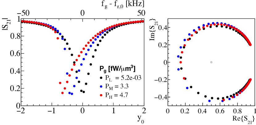
Figure 1: Frequency scan of the resonator at different generator powers $P_{g}$. Magnitude of the transmission $|S_{21}|$ as a function of the detuning in line-widths ($y_{0}$) (top, left), real and imaginary part of $S_{21}$ (top, right), and decay time of the pulses $\tau_{d}$ as a function of $y_{0}$ (bottom); Inset: $\delta\phi$ average pulses at low and medium powers with $y_{0}\sim 0$, and at high power with $y_{0}$ corresponding to the maximum of the $\tau_{d}$ overshoot.

In order to excite the resonator, the light from a room-temperature pulsed LED is driven to one side of the silicon substrate by an optical fiber passing through the cryostat. The absorbed light is converted to phonons in the silicon, which scatter through the lattice until they are absorbed in the superconductor and break the Cooper pairs. The pair-breaking alters the resonator frequency and quality factor, which are in turn measured through the phase ($\delta\phi$) and amplitude ($\delta A$) variations of the wave transmitted past the resonator relative to the center of the $S_{21}$ circle (see e.g. Zmuidzinas (2012)). Pulses following the optical excitation are acquired with a software trigger and averaged over around 500 samples to reduce noise in the estimation of their shape. The rise time of the pulses is dominated by the ring time of the resonator ($Q/\pi f_{r}=12\leavevmode\nobreak\ \mu s$) and by the phonon life-time in the substrate ($\sim 15\leavevmode\nobreak\ \mu s$), while the decay time is attributed to the relaxation of quasiparticles Martinez et al. (2019). The duration of the LED excitation is $2\leavevmode\nobreak\ \mu$s, and does not contribute significantly to the shape of the pulses.

The decay time $\tau_{d}$ of the pulses, measured as the time difference between the 90% and the 30% of their trailing edge, is shown in the bottom panel of Fig. 1 as a function of the detuning $y_{0}$. At low power $\tau_{d}$ does not depend on $y_{0}$ and averages to $0.64$ ms. The dependency is instead sizeable at medium and high powers, and in the latter case it varies from a minimum of $0.21$ to a maximum of $2.8$ ms. The overshoot at high power is found to be very narrow, around $0.006$ line-widths corresponding to 160 Hz in our case, and is therefore unlikely to spot if not intentionally searched for.
In the following we present a model which guided us in the measurement of the presented data and which is used in this work to identify origin and amount of the non-linearity. We begin with the study of the frequency sweeps and then move to the decay time of the pulses.

When $N_{qp}$ quasiparticles are created via pair-breaking, before recombining they store an amount of energy

$$E_{qp}=N_{qp}\Delta$$ (1)

where $2\Delta$ is the binding energy of a Cooper pair. In superconducting resonators the presence of quasiparticles, to a first-order approximation, modifies resonant frequency $f_{r}$ and quality factor $Q$ with respect to their low-power and low-temperature values ($f_{r,0},Q_{0}$) as:

$$x_{r} = -\alpha\frac{E_{qp}}{E^{\prime}}$$ (2)

$$\frac{1}{Q} = \frac{1}{Q_{0}}+2\frac{\alpha}{\beta}\frac{E_{qp}}{E^{\prime}}$$ (3)

where $x_{r}=({f_{r}-f_{r,0}})/{f_{r,0}}$, $\beta/2$ is the ratio between the frequency and inverse quality factor responses and $E^{\prime}$ is expected to be of the order of the pairing energy of the superconductor. The measurable quantity is the transmission $S_{21}$ which, for the resonator under study, can be expressed as Zmuidzinas (2012):

$$S_{21}=1-\frac{Q}{Q_{c}}\frac{1}{1+2jQx}$$ (4)

where $Q_{c}$ is the coupling quality factor and $x=(f_{g}-f_{r})/f_{r}$ is the detuning of the generator frequency with respect to $f_{r}$. In turn $x$ can be expressed in terms of the detuning $x_{0}$ with respect to $f_{r,0}$, $x_{0}=(f_{g}-f_{r,0})/f_{r,0}$, as:

$$x\simeq x_{0}+\alpha\frac{E_{qp}}{E^{\prime}}$$ (5)

where in the calculation we approximated $1+x_{r}\simeq 1$.

The energy absorbed in quasiparticles from the readout power amounts to Zmuidzinas (2012); de Visser et al. (2014):

$$E_{qp}^{P} = \eta_{g}P_{qp}\tau_{qp}$$ (6)

$$P_{qp} = P_{g}\frac{2Q^{2}}{Q_{c}Q_{qp}}\frac{1}{1+4Q^{2}x^{2}}$$ (7)

where $\eta_{g}$ is the efficiency in the creation of quasiparticles de Visser et al. (2012) , $\tau_{qp}$ and $Q_{qp}$ are the recombination time and the internal quality factor of quasiparticles, respectively. We finally define the non-linearity parameter as:

$$a_{qp}=\alpha Q\frac{E_{qp}^{P}(x=0)}{E^{\prime}}$$ (8)

The energy $E_{qp}^{P}$, may represent only a fraction of the total absorbed energy $E^{P}$ and thus of the non-linearity. In our device the total non-linearity ($a$) manifests itself in the non-linearity of the kinetic inductance, which has been already extensively studied Swenson et al. (2010); Zmuidzinas (2012):

$$a=\alpha Q\frac{E^{P}}{E^{\prime}}=\alpha\frac{2Q^{3}}{Q_{c}}\frac{P_{g}}{2\pi f_{r,0}}\frac{\gamma}{E^{\prime}}$$ (9)

where $\gamma$ is dimensionless parameter of order 1 to account for a possible difference in the energy scale. Defining $y=Qx$, we can rewrite Eqns. 5 and 3 in terms of $a$ and $a_{qp}$ as:

$$y = y_{0}z+\frac{a_{0}z^{3}}{1+4y^{2}}$$ (10)

$$z = \frac{Q}{Q_{0}}=1-\frac{2}{\beta}\frac{a_{qp,0}z^{3}}{1+4y^{2}}$$ (11)

where $a_{0}=a(Q=Q_{0})$ and $a_{qp,0}=a_{qp}(Q=Q_{0})$. These equations describe the detuning in line-widths with respect to the power-shifted resonant frequency ($y$), and the fractional change of the quality factor ($z$) as a function of $y$, respectively. It has to be underlined that the detuning is affected by the total non-linearity ($a$), while the quality factor is affected only by the portion of non-linearity due to quasiparticles ($a_{qp}$).

The values of ($z,y$) in Eq. 10 are calculated from the $S_{21}$ data (cf. Suppl. Mat.) and shown in Fig. 2 (left). At low-power the value of $z$ decreases with $|y|$, which reveals that the quality factor is dominated by TLS as it lowers with decreasing absorbed power. At higher powers the same behavior is observed at high $|y|$, while for $|y|$ around zero it decreases because of the power-generated quasiparticles. It has to be noticed that, at least for the resonator under study, the $z$ variation with $y$ at fixed power is only at few % level, presumably because of a compensation between the quality factors of quasiparticles and TLS. If quasiparticles had dominated the quality factor, we could have used Eq. 11 to extract $a_{qp,0}$ from fits to the $(z,y)$ data, provided that $\beta$ is measured independently. Nevertheless, as it will be shown next, it is possible to estimate $a_{qp,0}$ directly from the decay-time of the pulses, without introducing the effect of TLS in the model, and thus other free parameters.

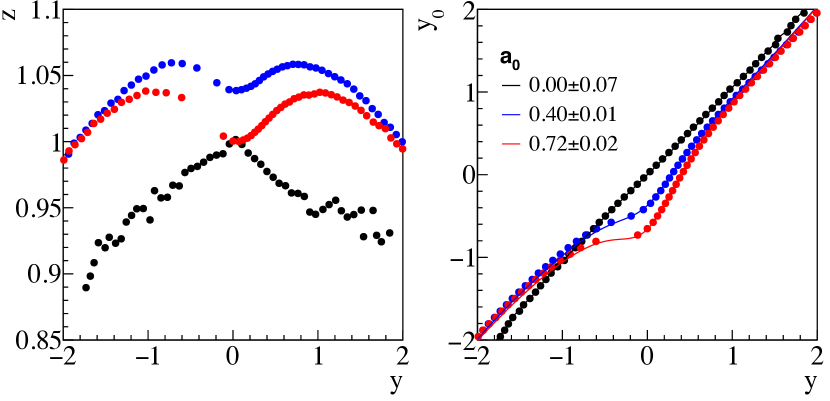
Figure 2: Left: $z=Q/Q_{0}$ as a function of the detuning with respect to the power-shifted resonant frequency ($y$) at low (black), medium (blue) and high (red) powers; Right: $y_{0}$ as a function of $y$ (dots) along with fits for $a_{0}$ of Eq. 10 (lines).

The points in the ($y,y_{0}$) plane are shown in Fig. 2 (right) along with fits of Eq. 10 for $a_{0}$ and using values of $z$ from the $(z,y)$ graph. The results are $a_{0}=0.00\pm 0.07,0.40\pm 0.01$ and $0.72\pm 0.02$ for the low, medium and high powers, respectively, with a 6% systematic error added from the model (cf. Suppl. Mat.).
The presence of a population of quasiparticles at equilibrium, along the frequency and quality factor of the resonator in Eqns. 2 and 3, modifies the recombination time as $\tau_{qp}\propto 1/N_{qp}$ Kaplan et al. (1976). One can therefore map the recombination time and the shift of the resonant frequency as:

$$\frac{1}{\tau_{qp}}=\frac{1}{\tau_{qp,0}}-\frac{y_{r}}{\tau_{k}}$$ (12)

where $\tau_{k}$ embeds the physics governing the dependency of frequency and recombination time with $N_{qp}$, $\tau_{qp,0}$ is the saturation value of the recombination time at low-power and low-temperature Barends et al. (2008), and

$$y_{r}=-\frac{a_{qp,0}z^{3}}{1+4y^{2}}$$ (13)

is the shift of the resonant frequency due to the power absorbed in quasiparticles.

When there are $M$ quasiparticles out of equilibrium, as in the case of excitation with the light pulses, their time evolution can be described as

$$\frac{dM}{dt}=-\frac{M}{\tau_{qp}}\left(1-\frac{\delta N^{P}_{qp}}{M}\right)$$ (14)

where the first term of the product accounts for the recombination, while the second for the extra quasiparticles $\delta N^{P}_{qp}$ injected or removed by the variation of the absorbed power. With a first order approximation  we obtain from Eq. 6:

$$\frac{\delta N^{P}_{qp}}{M} = \frac{\delta E^{P}_{qp}}{M\Delta}=-\frac{\delta x}{\delta x_{qp}}a_{qp}{F(y)}$$ (15)

$$F(y) = \frac{8y}{(1+4y^{2})^{2}}+\frac{\delta Q^{-1}}{\delta x}\frac{2}{(1+4y^{2})^{2}}$$ (16)

where $\delta x$ and $\delta Q^{-1}$ are the variations in detuning and inverse quality factor following the excitation, respectively, $\delta x_{qp}=\alpha M\Delta/E^{\prime}$ is the contribution to $\delta x$ due only to quasiparticles, $F(y)$ accounts for the feedback sign and dependency on $y$, and $a_{qp}$ accounts for its intensity.

Putting together Eqns. 14 and 15 we obtain the expression for the relaxation time:

$$\tau_{rel}=\frac{\tau_{qp}}{1-\frac{\delta N^{P}_{qp}}{M}}=\frac{\tau_{qp}}{1+\frac{\delta x}{\delta x_{qp}}a_{qp}F(y)}$$ (17)

In presence of quasiparticles’ non-linearity only, $\delta x/\delta x_{qp}=1$ and $\delta Q^{-1}/\delta x=2/\beta$. Other non-linearities, however, alter these parameters by adding a dependency on $y$. Including these effects would add free parameters to the model, therefore we chose to estimate $\delta x$ and $\delta Q^{-1}/\delta x$ directly from the $\delta\phi$ and $\delta A$ pulses acquired at each $y$ (cf. Suppl. Mat.). The value of $\delta x_{qp}$ is estimated from the pulses at high $|y|$, where the non-linearities are suppressed.

We fit the measured decay time of signals as a function of $y$ with $\tau_{qp,0},\tau_{k}$ and $a_{qp,0}$ as free parameters (Fig. 3). From the figure one can see that the first-order model we proposed reproduces well the data with $a_{qp,0}=0.27\pm 0.01$ and $a_{qp,0}=0.52\pm 0.01$ for the medium and high powers, respectively. We note that $a_{qp}/a=a_{qp,0}/a_{0}=(68\pm 3)\leavevmode\nobreak\ \%$ and $(72\pm 3)\leavevmode\nobreak\ \%$ for the the medium and high powers, respectively, pointing to the fact that quasiparticles account for a large fraction of the total non-linearity. Combining the two measurements and including the systematic error from the model we obtain $a_{qp}/a=(70\pm 5)\leavevmode\nobreak\ \%$.

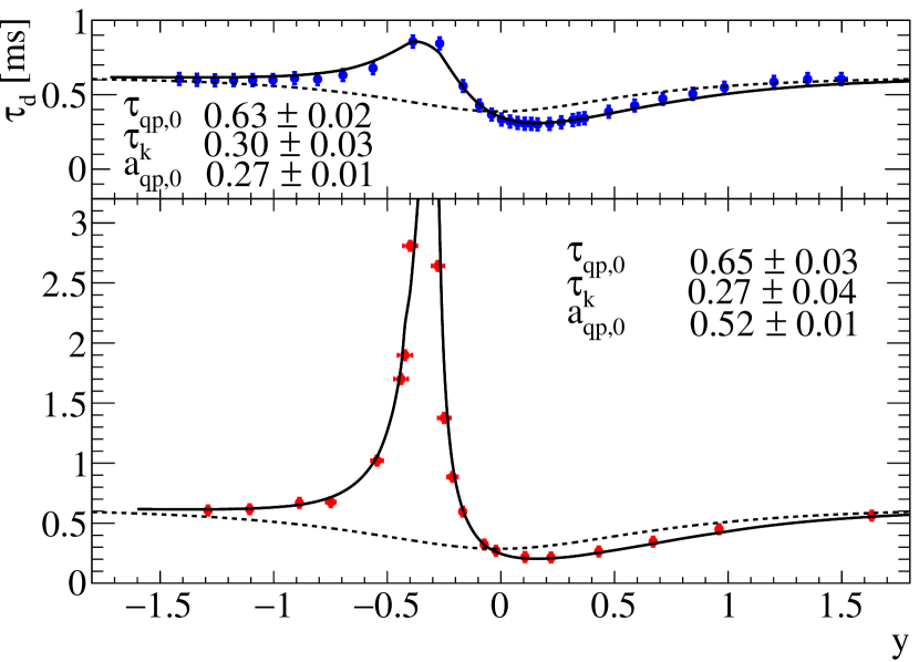
Figure 3: Decay time of the pulses ($\tau_{d}$) as a function of the power-shifted detuning ($y$) for the medium (top) and high (bottom) powers. The solid lines are fits of the model for the relaxation time including feedback effects (Eq. 17). The dashed lines indicate the contribution to these fits due to the steady change of $\tau_{qp}$ with absorbed power (Eq. 12) .

In order to deepen the understanding of the observed phenomena, we also study the variation of the decay time with temperature when the resonator is biased at low power. By doing this, we remove the generator feedback and, isolate the behaviour of $\tau_{qp}$ with a steady population of quasiparticles. Figure 4 shows the resonance shift with temperature (top) and the decay time as a function of the resonant frequency shift (bottom). Fitting Eq. 12 to the data points we find $\tau_{qp,0}=0.64\pm 0.01$ and $\tau_{k}=0.32\pm 0.01$ ms, which are in agreement with the values found from the power-generated quasiparticles in Fig 3.

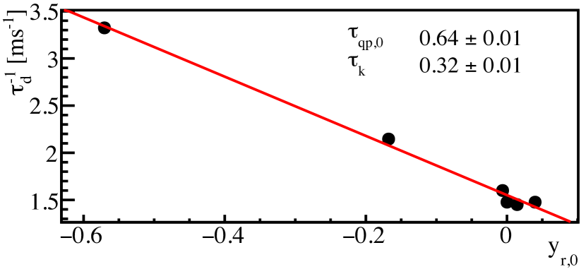
Figure 4: Temperature and frequency scan of the resonator at low generator power. Magnitude of the transmission $|S_{21}|$ as a function of $y_{0}$ (top) and inverse of the decay time of the signals $\tau_{d}$ as a function of the shift of the resonant frequency in line-widths ($y_{r,0}$) at each temperature (bottom). The solid line is a fit for Eq. 12.

The ratio of quasiparticles’ (Eq. 8) to total (Eq. 9) non-linearities,

$$\frac{a_{qp}}{a}=\frac{\eta_{g}}{\gamma}\frac{2\pi f_{r,0}\tau_{qp}}{Q_{qp}}\,,$$ (18)

allows in principle to derive $\eta_{g}/\gamma$, provided that $Q_{qp}$ is known at least to some approximation. From the definition of the total quality factor, $Q^{-1}=Q_{c}^{-1}+Q_{i}^{-1}$, and assuming that the internal quality factor, $Q_{i}$, is dominated by TLS and quasiparticles, ${Q_{i}}^{-1}\simeq{Q_{TLS}}^{-1}+Q_{qp}^{-1}$, we can argue that the maxima of $z$ in the frequency sweeps of Fig. 2 (left) correspond to $Q_{TLS}\simeq Q_{qp}$. The value of $Q_{qp}$ can be therefore estimated as:

$$\frac{1}{Q_{qp}}\Bigr{|}_{z_{\rm max}}\simeq\frac{1}{2}\left(\frac{1}{z_{\rm max}Q_{0}}-\frac{1}{Q_{c}}\right)$$ (19)

Using the values of $\tau_{qp}$ calculated with Eqns. 12 and  13 in the point $(y|z_{max},z_{max})$ and the measured value of $Q_{c}$ ($Q_{c}=115100$, cf. Suppl .Mat.), from Eq. 18 we obtain $\eta_{g}/\gamma=(18\pm 3)\leavevmode\nobreak\ \%$ and $(16\pm 3)$ % for the medium and high power data, respectively. Assuming $\gamma=1$, the value of $\eta_{g}$ is in line with the predictions in Ref. Goldie and Withington (2013).
Our results reveal the existence of a population of quasiparticles generated from the readout power which undergoes a strong electro-thermal feedback and which significantly modifies the properties of the superconducting circuit. As an example, the positive feedback could be exploited to increase the response of superconducting circuits at signal frequencies below $1/2\pi\tau_{rel}$ . The negative feedback, instead, could be exploited to make the circuit more resistant to quasiparticles’ perturbations. Materials with different intrinsic values of $\tau_{qp}/Q_{qp}$ could be studied to enhance or suppress the non-linearity from quasiparticles.
The authors acknowledge useful discussion with J. Lorenzana, A. Monfardini and I. M. Pop, and thank the personnel of INFN Sezione di Roma for the technical support, in particular A. Girardi and M. Iannone. This work was supported by the European Research Council (FP7/2007-2013) under Contract No. CALDER 335359 and by the Italian Ministry of Research under the FIRB Contract No. RBFR1269SL.

References

- Martinis et al. (1985) J. M. Martinis, M. H. Devoret, and J. Clarke, Phys. Rev. Lett., 55, 1543 (1985).
- Feldman et al. (1975) M. J. Feldman, P. T. Parrish, and R. Y. Chiao, Journal of Applied Physics, 46, 4031 (1975).
- Dolan et al. (1979) G. J. Dolan, T. G. Phillips, and D. P. Woody, Applied Physics Letters, 34, 347 (1979).
- Day et al. (2003) P. K. Day, H. G. LeDuc, B. A. Mazin, A. Vayonakis, and J. Zmuidzinas, Nature, 425, 817 (2003).
- Ho Eom et al. (2012) B. Ho Eom, P. K. Day, H. G. LeDuc, and J. Zmuidzinas, Nature Physics, 8, 623 (2012).
- Faramarzi et al. (2021) F. B. Faramarzi et al., (2021), arXiv:2012.08654 .
- Kaplan et al. (1976) S. B. Kaplan, C. C. Chi, D. N. Langenberg, J. J. Chang, S. Jafarey, and D. J. Scalapino, Phys. Rev. B, 14, 4854 (1976).
- Martinis et al. (2005) J. M. Martinis, K. B. Cooper, R. McDermott, M. Steffen, M. Ansmann, K. D. Osborn, K. Cicak, S. Oh, D. P. Pappas, R. W. Simmonds, and C. C. Yu, Phys. Rev. Lett., 95, 210503 (2005).
- McRae et al. (2020) C. R. H. McRae, H. Wang, J. Gao, M. R. Vissers, T. Brecht, A. Dunsworth, D. P. Pappas, and J. Mutus, Review of Scientific Instruments, 91, 091101 (2020).
- De Visser et al. (2014) P. De Visser, J. Baselmans, J. Bueno, N. Llombart, and T. Klapwijk, Nature Communications, 3 (2014).
- de Visser et al. (2010) P. J. de Visser, S. Withington, and D. J. Goldie, Journal of Applied Physics, 108, 114504 (2010).
- Thompson et al. (2013) S. E. Thompson, S. Withington, D. J. Goldie, and C. N. Thomas, Superconductor Science and Technology, 26, 095009 (2013).
- Thomas et al. (2015) C. N. Thomas, S. Withington, and D. J. Goldie, Superconductor Science and Technology, 28, 045012 (2015).
- Cardani et al. (2017) L. Cardani, N. Casali, I. Colantoni, A. Cruciani, F. Bellini, M. G. Castellano, C. Cosmelli, A. D’Addabbo, S. Di Domizio, M. Martinez, C. Tomei, and M. Vignati, Appl. Phys. Lett., 110, 033504 (2017).
- Swenson et al. (2010) L. J. Swenson, A. Cruciani, A. Benoit, M. Roesch, C. S. Yung, A. Bideaud, and A. Monfardini, Appl. Phys. Lett., 96, 263511 (2010).
- Bourrion et al. (2013) O. Bourrion, C. Vescovi, A. Catalano, M. Calvo, A. D’Addabbo, J. Goupy, N. Boudou, J. F. Macias-Perez, and A. Monfardini, JINST, 8, C12006 (2013).
- Khalil et al. (2012) M. S. Khalil, M. J. A. Stoutimore, F. C. Wellstood, and K. D. Osborn, J. Appl. Phys., 111, 054510 (2012).
- Swenson et al. (2013) L. Swenson, P. K. Day, B. H. Eom, H. G. LeDuc, N. Llombart, C. M. McKenney, O. Noroozian, and J. Zmuidzinas, J. Appl. Phys., 113, 104501 (2013).
- Zmuidzinas (2012) J. Zmuidzinas, Annu.Rev.Cond.Mat.Phys., 3, 169 (2012).
- Martinez et al. (2019) M. Martinez, L. Cardani, N. Casali, A. Cruciani, G. Pettinari, and M. Vignati, Phys. Rev. Applied, 11, 064025 (2019).
- de Visser et al. (2014) P. J. de Visser, D. J. Goldie, P. Diener, S. Withington, J. J. A. Baselmans, and T. M. Klapwijk, Phys. Rev. Lett., 112, 047004 (2014).
- de Visser et al. (2012) P. J. de Visser, J. J. A. Baselmans, S. J. C. Yates, P. Diener, A. Endo, and T. M. Klapwijk, Appl. Phys. Lett., 100, 162601 (2012).
- Note (1) depends on the number of quasiparticles, and thus on Goldie and Withington (2013). This dependency can be neglected in our first-order model.
- Barends et al. (2008) R. Barends, J. J. A. Baselmans, S. J. C. Yates, J. R. Gao, J. N. Hovenier, and T. M. Klapwijk, Phys. Rev. Lett., 100, 257002 (2008).
- Note (2) In the calculation of derivative, we approximated since the dependency of and on the number of quasiparticles cancels to a good approximation de Visser et al. (2012).
- Goldie and Withington (2013) D. J. Goldie and S. Withington, Superconductor Science and Technology, 26, 015004 (2013).