Dynamic VNF Placement, Resource Allocation and Traffic Routing in 5G

Abstract

5G networks are going to support a variety of vertical services, with a diverse set of key performance indicators (KPIs), by using enabling technologies such as software-defined networking and network function virtualization. It is the responsibility of the network operator to efficiently allocate the available resources to the service requests in such a way to honor KPI requirements, while accounting for the limited quantity of available resources and their cost. A critical challenge is that requests may be highly varying over time, requiring a solution that accounts for their dynamic generation and termination. With this motivation, we seek to make joint decisions for request admission, resource activation, VNF placement, resource allocation, and traffic routing. We do so by considering real-world aspects such as the setup times of virtual machines, with the goal of maximizing the mobile network operator profit. To this end, first, we formulate a one-shot optimization problem which can attain the optimum solution for small size problems given the complete knowledge of arrival and departure times of requests over the entire system lifespan. We then propose an efficient and practical heuristic solution that only requires this knowledge for the next time period and works for realistically-sized scenarios. Finally, we evaluate the performance of these solutions using real-world services and large-scale network topologies. Results demonstrate that our heuristic solution performs better than state-of-the-art online algorithms and close to the optimum.

Sec. I Introduction

5G networks are envisioned to support a variety of services belonging to vertical industries (e.g., autonomous driving, media, and entertainment) with a diverse set of requirements. Services are defined as a directed graph of virtual network functions (VNFs) with specific and varying key performance indicators (KPIs), e.g., throughput, and delay. Requests for these services arrive over time and mobile network operators (MNOs) are responsible for efficiently satisfy such a demand, by fulfilling their associated KPI while minimizing the cost for themselves.

As a result of the softwarization of 5G-and-beyond networks, enabled by software-defined networking (SDN) and network function virtualization (NFV), it is now feasible to use general-purpose resources (e.g., virtual machines) to implement the VNFs required by the different service. The decision on which resources to associate with which VNF and service is made by a network component called orchestrator, as standardized by ETSI [1]. Without loss of generalityi, we focus only on computational and communication resources (e.g., virtual machines and the links connecting them); notice, however, that our proposed framework is applicable to other resource types (e.g., storage).

The network orchestrator makes the following decisions [1]:

• admission of requests;

• activation/deactivation of VMs;

• placement of VNF instances therein;

• assignment of CPU to VMs for running the hosted VNF instances;

• routing of traffic through physical links.

These decisions are clearly mutually dependent, and therefore should be made jointly, in order to account for the – often nontrivial – ways in which they influence one another. The focus of this paper is thus to consider the joint requests admission, VM activation/deactivation, VNF placement, CPU assignment, and traffic routing problem in order to maximize the MNO profit, while considering:

• the properties of each VNF,

• the KPI requirements of each service,

• the capabilities of VMs and PoPs (points of presence, e.g., datacenters) and their latency,

• the capacity and latency of physical links,

• the VMs setup times,

• the arrival and departure times of service requests.

As better discussed in Sec. II, some of these factors are simplified, or even neglected, in existing works on 5G orchestration. Notably, we account for the VM setup time, which becomes a significant factor in (for example) IoT applications, when requests are often short-lived. Ignoring setup (and tear-down) times can reduce the optimality of existing solutions.

Furthermore, we account for the fact that different VNFs may have different levels of complexity, therefore, different quantities of computational resources may be needed to attain the same KPI target. Inspired by several works in the literature [2], we model individual VNFs as queues and services as queuing networks. Critically, unlike traditional queuing networks, the quantity of traffic (i.e., the number of clients in queues) can change across queues, as VNFs can drop some packets (e.g., firewalls) or change the quantity thereof (e.g., video transcoders). Our model accounts for this important aspect by replacing traditional flow conservation constraints with a generalized flow conservation law, allowing us to describe arbitrary services with arbitrary VNF graphs.

Given this model, we formulate a one-shot optimization problem which, assuming perfect knowledge of future requests, allows us to maximize the MNO profit. Given the NP-hardness of such a problem and the fact that knowledge of future requests is usually not available, we propose MaxSR, an efficient heuristic algorithm which will be invoked periodically based on the knowledge of requests within each time period. The proposed method can achieve a near-optimal solution for large-scale network scenarios. We evaluate MaxSR compared to the optimum and other benchmarks using real-world services and different network scenarios.

In summary, the main contributions of this paper are as follows:

• we propose a complete model for the main components of 5G, both in terms of vertical services (dynamic requests, VNFs, and services KPIs) and in terms of resources (e.g. VMs and links);

• our model accounts for the time variations of service requests, and dynamically allocates the computational and network resources while considering VMs setup times. It can also accommodate a diverse set of VNFs in terms of computational complexity and KPI requirements, multiple VNF instances, and arbitrary VNF graphs with several ingress and egress VNFs, rather than a simple chain or directed acyclic graph (DAG);

• we formulate a one-shot optimization problem as a Mixed-Integer Programming (MIP) to make a joint decision on VM state, VNF placement, CPU assignment, and traffic routing based on the complete requests statistics over the entire system lifespan;

• we propose MaxSR, an efficient near-optimal heuristic algorithm to solve the aforementioned problem based on the knowledge of the near future for large scale network scenarios;

• finally, we compare MaxSR with optimum and the online approach Best-Fit, through extensive experiments using synthetic services and requests, and different network scenarios.

The rest of the paper is organized as follows. Sec. II reviews related works. Sec. III describes the system model and problem formulation, while Sec. IV clarifies our solution strategy. Finally, Sec. V presents our numerical evaluation under different network scenarios, and Sec. VI concludes the paper.

Sec. II Related Work

Several works have addressed VNF placement and traffic routing, as exemplified by the survey paper [3]. In most of these works, the problem is formulated as a Mixed Integer Linear Program (MILP) with a different set of objectives and constraints. Such an approach can yield exact solutions, but merely works for small instances; therefore, heuristic algorithms that offer a near-optimal solution have also been presented.

In particular, a first body of works provides a one-time VNFs placement, given the incoming service requests. Since this method leaves already placed VNFs intact, it can lead to a sub-optimal solution when the traffic varies over time. Examples of such an approach can be found in [4, 5, 6, 7, 8, 9], which aim at minimizing a cost function, e.g., operational cost, QoS degradation cost, server utilization, or a combination of them, and assume that there are always enough resources to serve the incoming requests. Among them, Cohen et al. [4] propose an approximation algorithm to place sets of VNFs in an optimal manner, while approximating to the constraints by a constant factor. Pham et al. [7] introduce a distributed solution based on a Markov approximation technique to place chains of VNFs where the cost enfolds the delay cost, in addition to the cost of traffic and server. [8], instead, addresses the same problem but aims at minimizing the energy consumption, given constraints on end-to-end latency for each flow and server utilization. Pei et al. [9] propose an online heuristic for this problem, by which VNF instances are deployed and connected using the shortest path algorithm, in order to minimize the number VNF instances and satisfy their end-to-end delay constraint.

Another thread of works focuses on an efficient admission policy that maximizes the throughput or revenue of admitted requests [10, 11, 12, 13]. In particular, Sallam et al. [10] formulate joint VNF placement and resource allocation problem to maximize the number of fully served flows considering the budget and capacity constraints. They leverage the sub-modularity property for a relaxed version of the problem and propose two heuristics with a constant approximation ratio. [11] studies the joint VNF placement and service chain embedding problem, so as to maximize the revenue from the admitted requests. A similar problem is tackled in [13] and [12] but for an online setting where the requests should be admitted and served upon their arrival. Zhou et al. [12], on the other hand, first formulate a one-shot optimization problem over the entire system lifespan and then leverage the primal-dual method to design an online solution with a theoretically proved upper bound on the competitive ratio.

A different approach is adopted in [14, 15, 16, 17, 18, 19, 20] where VNF placement can be readjusted through VNF sharing and migration, to optimally fit time-varying service demands. [14] and [15] propose algorithms that properly scale over-utilized or under-utilized VNF instances based on the estimation of future service demands. Jia et al. [16] propose an online algorithm with a bounded competitive ratio that dynamically deploys delay constrained service function chains across geo-distributed datacenters minimizing operational costs.

Request admission control has instead been considered in [17, 18, 19, 20]. More in detail, Li et al. [17] propose a proactive algorithm that dynamically provisions resources to admit as many requests as possible with a timing guarantee. Similarly, [18] admits requests and places their VNFs in the peak interval, but minimizes the energy cost of VNF instances by migration and turning off empty ones in the off-peak interval. Liu et al. [19] envision an algorithm that maximizes the service provider’s profit by periodically admitting new requests and rearranging the current-served ones, while accounting for the operational overhead of migration. Finally, leveraging VNF migration and sharing, [20] proposes an online algorithm to maximize throughput while minimizing service cost and meeting latency constraints.

Relevant to our work are also studies that target specifically 5G systems, although they merely consider the link delay and neglect processing delays in the servers. An example can be found in [2], which models VMs as M/M/1 PS queues, and proposes a MILP and a heuristic solution to minimize the average service delay, while meeting the constraints on the links and host capacities. The works in [21] and [22] aim instead to minimize, respectively, the operational cost and the energy consumption of VMs and links while ensuring end-to-end delay KPI. [22] also allows for VNF sharing and studies the impact of applying priorities to different services within a shared VNF. Zhang et al. [23] tackle the request admission problem to maximize the total throughput, neglecting instead queuing delay at VMs.

We remark that most of the above works present proactive approaches, and only deal with either cost minimization or request admission. On the contrary, we focus on dynamic resource activation, VNF placement, and CPU assignment to maximize the revenue from admitted requests over the entire system lifespan, while minimizing the deployment costs and accounting for some practical issues. Our proactive MILP formulation of the problem extends existing models by accounting for the maximum end-to-end delay as the main KPI, while our heuristic is a practical and scalable solution, which periodically admits new requests and readjusts the existing VNF deployment. To the best of our knowledge, this is the first dynamic solution for service orchestration in 5G networks.

Sec. III System Model and Problem Formulation

In this section, first we describe our system model supported by a simple example. Later, we formulate the joint requests admission, VM activation, VNF placement, CPU assignment, and traffic routing problem; a discussion of the problem time complexity follows. The frequently used notation is summarized in Table I.

TABLE I: Notation (sets, variables, and parameters)

Symbol Description $\mathcal{D}$ Set of datacenters $\mathcal{E}$ Set of physical links $\mathcal{K}$ Set of service requests $\mathcal{L}$ Set of logical links $\mathcal{M}$ Set of VMs $\mathcal{P}$ Set of end-to-end paths $\mathcal{Q}$ Set of VNFs $\mathcal{S}$ Set of services $\mathcal{T}$ Set of time steps $\mathcal{W}_{s}$ Set of paths from ingress VNFs to egress VNFs in VNF graph of service $s$ $A(k,m,q,t)$ Whether to deploy VNF $q$ of service request $k$ at VM $m$ at time $t$ $D(k,m,q,t)$ Traffic departing VM $m$ for VNF $q$ of service request $k$ at time $t$ $F(k,l,q_{1},q_{2},t)$ Equal to $1$ when $\rho(k,l,q_{1},q_{2},t)>0$ $I(k,m,q,t)$ Traffic entering VM $m$ for VNF $q$ of service request $k$ at time $t$ $L(e,t)$ Traffic on physical link $e$ at time $t$ $O(m,t)$ Whether VM $m$ is active at time $t$ $R(m,t)$ Average time for a request to be processed at VM $m$ at time $t$ $U(m,t)$ Whether VM $m$ is turning-on at time $t$ $V(k,t)$ Whether service request $k$ is active at time $t$ $\mu(k,m,q,t)$ Service rate to assign to VM $m$ for VNF $q$ of service request $k$ at time $t$ $\rho(k,l,q_{1},q_{2},t)$ Fraction of traffic from VNF $q_{1}$ to $q_{2}$ of service request $k$, through logical link $l$ at time $t$

Symbol Description $B(e)$ Bandwidth of physical link $e$ $C_{\textit{dc}}(d)$ Computational capacity of datacenter $d$ $C_{\textit{vm}}(m)$ Computational capacity of VM $m$ $D_{\textit{QoS}}(s)$ Target delay for service $s$ $D_{\textit{log}}(l)$ Delay of logical link $l$ $D_{\textit{phy}}(e)$ Delay of physical link $e$ $N(s,q)$ Maximum number of instances for VNF $q$ of service $s$ $X_{\textit{cpu}}(m)$ Cost for VM $m$ to process one unit of computation in one time step $X_{\textit{idle}}(m)$ Fixed cost incurred when VM $m$ is turning-on or active in one time step $X_{\textit{link}}(e)$ Cost of data transmission through physical link $e$ in one time step $X_{\textit{rev}}(s)$ Revenue from serving one traffic unit of service $s$ $\Lambda(s,q_{1},q_{2})$ Traffic from VNF $q_{1}$ to $q_{2}$ for service $s$ $\mathds{P}(s,q_{1},q_{2})$ Probability that traffic processed at VNF $q_{1}$ is forwarded to VNF $q_{2}$ of service $s$ $\alpha(s,q)$ Ratio of outgoing traffic to incoming traffic for VNF $q$ of service $s$ $\lambda_{\textit{new}}(s)$ New traffic for service $s$ $\omega(q)$ Computation capability required for one traffic unit at VNF $q$ $t_{\textit{arv}}(k)$ Arrival time of service request $k$ $t_{\textit{dpr}}(k)$ Departure time of service request $k$

III-A System Model

Physical infrastructure. Let $\mathcal{G}=(\mathcal{M},\mathcal{E})$ be a directed graph representing the physical infrastructure network, where each node $m\in\mathcal{M}$ is either a VM or a network node (i.e., a router or a switch). A VM $m$ has maximum computational capacity $C_{\textit{vm}}(m)$. Set $\mathcal{E}$ denotes the physical links connecting the network nodes. We define $B(e)$ and $D_{\textit{phy}}(e)$ as, respectively, the bandwidth and delay of physical link $e\in\mathcal{E}$. Time is discretized into steps, $\mathcal{T}=\{1,2,…,T\}$, and we assume that at every time step a VM may be in one of the following states: terminated, turning-on, or active. Specifically, VMs can only be used when they are active, and they need to be turned-on one time step before being active. Based on the measurements reported in [15], we also consider the traffic flow migration time to be negligible with respect to the VM setup time.

Each VM can host one VNF and belongs to a datacenter $d\in\mathcal{D}$; we denote the available amount of computational resources in datacenter $d$ by $C_{\textit{dc}}(d)$ and the set of VMs within $d$ with $\mathcal{M}_{d}$. In the physical graph $G$, physical links within datacenters are assumed to be ideal, i.e., they have no capacity limit and zero delay. Let logical link $l\in\mathcal{L}$ be a sequence of physical links connecting two VMs, $\textit{src}(l)$ and destination $\textit{dst}(l)$, then we define end-to-end path $p\in\mathcal{P}$ as a sequence of logical links.

Services. We represent each service $s\in\mathcal{S}$ with a VNF Forwarding Graph (VNFFG), where the nodes are VNFs $q\in\mathcal{Q}$, and the directed edges show how traffic traverses the VNFs. VNFFG can be any general graph with possibly several ingress and egress VNFs. We denote the total new traffic, entering the ingress VNFs of service $s$, by $\lambda_{\textit{new}}(s)$. A traffic packet of service $s$, processed in VNF $q_{1}$, is forwarded to VNF $q_{2}$ with probability of $\mathds{P}(s,q_{1},q_{2})$. Similarly, $\mathds{P}(s,\circ,q)$ is the probability that a new traffic packet of service $s$ starts getting service in ingress VNF $q$, and $\mathds{P}(s,q,\circ)$ is the probability that a traffic packet of service $s$, already served at egress VNF $q$, departs service $s$. For each service $s$, we consider its target delay, $D_{\textit{QoS}}(s)$, as the most critical KPI, specifying the maximum tolerable end-to-end delay for the traffic packets of $s$.

VNFs can have different processing requirements depending on their computational complexity. We denote by $\omega(q)$ the computational capability that VNF $q$ needs to process one unit of traffic. Some VNFs may not find sufficient resources on a single VM to completely serve the traffic while satisfying the target delay. Thus, multiple instances can be created, with $N(s,q)$ being the maximum number of instances of VNF $q$ at each point in time. Instances of the same VNF can be deployed either within the same datacenter or at different datacenters; in the latter case, the traffic between each pair of VNFs must be splitted through different logical links that connect the VMs running the corresponding VNF instances.

Different requests for the same services may arrive over time; we denote with $K_{s}$ the set of all service requests for service $s$, and characterize the generic service request $k\in\mathcal{K}$ with its arrival time $t_{\textit{arv}}(k)$ and departure time $t_{\textit{dpr}}(k)$. Due to slice isolation requirements [24], we assume that the VNF instances of different service requests are not shared with other service requests.

(a)

(b)

(c)

Figure 1: VNFFG of LABEL:sub@fig:model-exm1 vehicle collision detection (VCD) service and LABEL:sub@fig:model-exm2 video on-demand (VoD) service. The number on edges represents transition probability of traffic packets. LABEL:sub@fig:model-exm3 Physical graph including three datacenters connected using a switch.

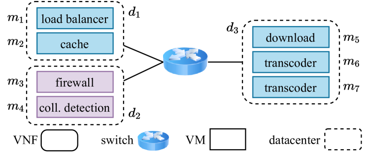
Example. Figure 1 represents a possible deployment of two sample services, vehicle collision detection (VCD) and video on-demand (VoD), on the physical graph (Figure 1c) in a single time step. VCD is a low-latency service with a very low target delay $D_{\textit{QoS}}$, and VoD is a traffic intensive service with a high $\lambda_{\textit{new}}$. Figure 1a and Figure 1b depict the VNFFGs of the VCD and VoD services, respectively, where the numbers on the edges represent the transition probability of traffic packets between corresponding VNFs. The physical graph contains a set of datacenters $\mathcal{D}=\{d_{1},d_{2},d_{3}\}$ with computational capability $C_{\textit{dc}}$. Datacenters are connected to each other using a switch and physical links with bandwidth $B$ and a latency $D_{\textit{phy}}$. VMs within each datacenter are denoted by sets $\mathcal{M}_{d_{1}}=\{m_{1},m_{2}\}$, $\mathcal{M}_{d_{2}}=\{m_{3},m_{4}\}$, and $\mathcal{M}_{d_{3}}=\{m_{5},m_{6},m_{7}\}$, each with computational capability $C_{\textit{vm}}$. As depicted in Figure 1c, service VCD is deployed within datacenter $d_{2}$ to avoid inter-datacenter network latency. Service VoD is deployed across datacenter $d_{1}$ and third-party datacenter $d_{3}$. VNF transcoder, having high computational complexity $\omega$, requires two instances in datacenters $d_{3}$ to fully serve the traffic.

III-B Problem Formulation

In this section, we first describe the decisions that have to be made to map the service requests onto network resources. Then we formalize the system constraints and the objective using the model presented in Sec. III-A, along with the decision variables we define. In general, given the knowledge of the future arrival and departure times of service requests, we should make the following decisions:

• service request activation, i.e., when service requests get served;

• VM activation/deactivation, i.e., when VMs are set up or terminated;

• VNF instance placement, i.e., which VMs have to run VNF instances;

• CPU assignment, i.e., how much computational capability shall be assigned to a VM to run the deployed VNF;

• traffic routing, i.e., how traffic between VNFs is routed through physical links.

Service request activation. Let binary variable $V(k,t)\in\{0,1\}$ denote whether service request $k$ is being served at time $t$. Once admitted, a service request has to be provided for all its lifetime duration. Given service request arrival time $t_{\textit{arv}}(k)$ and departure time $t_{\textit{dpr}}(k)$, this translates into:

$$V(k,t)=0,\hfill\forall k\in\mathcal{K},t\in\mathcal{T}:t<t_{\textit{arv}}(k)\vee t\geq t_{\textit{dpr}}(k).$$ (1)

VNF instances. The following constraint limits the number of deployed instances of VNF $q$ of any service request $k\in\mathcal{K}_{s}$ to be less than $N(s,q)$ at any point in time:

$$\sum_{m\in\mathcal{M}}{A(k,m,q,t)}\leq N(s,q),\\ \forall t\in\mathcal{T},s\in\mathcal{S},k\in\mathcal{K}_{s},q\in\mathcal{Q},$$ (2)

where binary variable $A(k,m,q,t)$ represents whether VNF $q$ of service request $k$ is placed on VM $m$ at time $t$. The network slice isolation property of 5G networks prevents VNF sharing among requests for different services. In addition, at most one VNF instance can be deployed on any VM, i.e.,

$$\sum_{k\in\mathcal{K}}{\sum_{q\in\mathcal{Q}}{A(k,m,q,t)}}\leq 1,\hfill\forall m\in\mathcal{M},t\in\mathcal{T}.$$ (3)

VM states. We define two binary variables $U(m,t)$ and $O(m,t)$ to represent whether VM $m$ is turning-on or active at time $t$, respectively. We formulate a simple constraint to prevent VMs from being concurrently turning-on and active at any time, i.e.,

$$O(m,t)+U(m,t)\leq 1,\hfill\forall m\in\mathcal{M},t\in\mathcal{T}.$$ (4)

The following constraint enforces that VM $m$ can be active at time $t$ only if it has been turning-on or active in the previous time step:

$$O(m,t)\leq O(m,t-1)+U(m,t-1),\hfill\forall m\in\mathcal{M},t\in\mathcal{T}.$$ (5)

VMs are able to run VNFs only when they are active, i.e.,

$$\sum_{k\in\mathcal{K}}{\sum_{q\in\mathcal{Q}}{A(k,m,q,t)}}\leq O(m,t),\hfill\forall m\in\mathcal{M},t\in\mathcal{T}.$$ (6)

Computational capacity. Let real variable $\mu(k,m,q,t)$ represent the service rate assigned to VM $m$ to run VNF $q$ of service request $k$ at time $t$. Multiplying it by $\omega(q)$, we have the amount of computation capability assigned to VM $m$ to run VNF $q$ at time $t$. The limited computational capability of datacenters and VMs denoted, respectively, by $C_{\textit{dc}}(d)$ and $C_{\textit{vm}}(m)$, should not be exceeded at any point in time. We describe such a limitation by imposing:

$$\sum_{m\in\mathcal{M}_{d}}{\sum_{k\in\mathcal{K}}{\sum_{q\in\mathcal{Q}}{\mu(k,m,q,t)\cdot\omega(q)}}}\leq C_{\textit{dc}}(d),\\ \forall t\in\mathcal{T},d\in\mathcal{D},$$ (7)

where the sum on the left-hand side of the inequality is over all VMs within datacenter $d$. Similarly, for the VMs we have

$$\mu(k,m,q,t)\cdot\omega(q)\leq A(k,m,q,t)\cdot C_{\textit{vm}}(m),\\ \forall t\in\mathcal{T},k\in\mathcal{K},q\in\mathcal{Q},m\in\mathcal{M},$$ (8)

where $A(k,m,q,t)$ on the right-hand side of the inequality enforces zero service rate for VM $m$ when no VNF is placed therein.

KPI target fulfillment. Whenever a service request is being served, i.e., $V(k,t)=1$, all the traffic in the corresponding VNFFG should be carried by the underlying physical links. The following constraint ensures this condition for the traffic between each pair of VNFs at any point in time:

$$\sum_{l\in\mathcal{L}}{\rho(k,l,q_{1},q_{2},t)}\geq V(k,t),\\ \forall t\in\mathcal{T},s\in\mathcal{S},k\in\mathcal{K}_{s},q_{1},q_{2}\in\mathcal{Q}:\mathds{P}(s,q_{1},q_{2})>0.$$ (9)

Real variable $\rho(k,l,q_{1},q_{2},t)$ shows the fraction of traffic from VNF $q_{1}$ to $q_{2}$ of service request $k$ that is routed through logical link $l$ at time $t$. As mentioned, the traffic flow from VNF $q_{1}$ to VNF $q_{2}$ may be splitted into several logical links (see Eq. (2)). Moreover, since we consider multi-path routing, there may be multiple logical links between each pair of VNF instances. Therefore, constraint (9) implies that for any service request $k$ requesting traffic from VNF $q_{1}$ to $q_{2}$ (i.e., $\mathds{P}(s,q_{1},q_{2})>0$), the sum of all fractional traffic going though any logical link, should be equal to $1$ at any time when the service request is being served.

The above constraint does not include ingress and egress traffic. To account for such contributions, we need to introduce dummy nodes in the VNFFG and the physical graph. We add an end-point dummy VNF, $\circ$ in every VNFFG, which is directly connected to all ingress and egress VNFs and a dummy VM in the physical graph which is directly connected to all VMs. We define $\mathcal{L}_{\circ}$ as the set of dummy logical links which start from or end at the dummy VM. We assume that dummy logical links are ideal, i.e., they have no capacity limit and zero delay and cost. We can now formulate the associated traffic constraints as:

$$\sum_{l\in\mathcal{L}_{\circ}}{\rho(k,l,\circ,q,t)}\geq V(k,t),\\ \forall t\in\mathcal{T},s\in\mathcal{S},k\in\mathcal{K}_{s},q\in\mathcal{Q}:\mathds{P}(s,\circ,q)>0,$$ (10)

$$\sum_{l\in\mathcal{L}_{\circ}}{\rho(k,l,q,\circ,t)}\geq V(k,t),\\ \forall t\in\mathcal{T},s\in\mathcal{S},k\in\mathcal{K}_{s},q\in\mathcal{Q}:\mathds{P}(s,q,\circ)>0,$$ (11)

where $\rho(k,l,\circ,q,t)$ and $\rho(k,l,q,\circ,t)$ are the fraction of new traffic entering ingress VNF $q$ and the fraction of traffic departing from egress VNF $q$, respectively, going through logical link $l$ at time $t$.

Placement. We can now correlate the routing decisions $\rho$ and the placement decisions $A$ as

$$\rho(k,l,q_{1},q_{2},t)\leq A(k,m,q_{2},t),\\ \forall t\in\mathcal{T},k\in\mathcal{K},q_{1}\in\mathcal{Q}\cup\{\circ\},q_{2}\in\mathcal{Q},\\ m\in\mathcal{M},l\in\mathcal{L}\cup\mathcal{L}_{\circ}:\textit{dst}(l)=m.$$ (12)

The above constraint implies that whenever there is an incoming traffic to VNF $q_{2}$ through logical link $l$ whose destination is VM $m$, i.e., $\textit{dst}(l)=m$, VNF $q_{2}$ is deployed at VM $m$. Similarly, whenever there is an outgoing traffic from VNF $q_{1}$ through logical link $l$ whose source is VM $m$, i.e., $\textit{src}(l)=m$, VNF $q_{1}$ is deployed at VM $m$:

$$\rho(k,l,q_{1},q_{2},t)\leq A(k,m,q_{1},t),\\ \forall t\in\mathcal{T},k\in\mathcal{K},q_{1}\in\mathcal{Q},q_{2}\in\mathcal{Q}\cup\{\circ\}\\ m\in\mathcal{M},l\in\mathcal{L}\cup\mathcal{L}_{\circ}:\textit{src}(l)=m.$$ (13)

System stability. Let $\lambda(s,q)$ denote the total incoming traffic of VNF $q$ of service $s$. $\lambda(s,q)$ equals the sum of ingress traffic and the traffic coming from other VNFs to VNF $q$ of service $s$:

$$\lambda(s,q)=\lambda_{\textit{new}}(s)\cdot\mathds{P}(s,\circ,q)+\\ +\sum_{q_{1}\in\mathcal{Q}\backslash\{q\}}{\lambda(s,q^{\prime})\cdot\mathds{P}(s,q^{\prime},q)}.$$ (14)

Using $\lambda(s,q)$, the amount of traffic from VNF $q_{1}$ to VNF $q_{2}$ of service $s$ can be represented as:

$$\Lambda(s,q_{1},q_{2})=\lambda(s,q_{1})\cdot\mathds{P}(s,q_{1},q_{2}).\hfill$$ (15)

We can now define an auxiliary variable to represent the incoming traffic of VNF $q$ of service request $k$, which enters VM $m$ at time $t$:

$$I(k,m,q,t)=\sum_{\begin{subarray}{c}q^{\prime}\in\mathcal{Q}\cup\{\circ\}\end{subarray}}{\sum_{\begin{subarray}{c}l\in\mathcal{L}\cup\mathcal{L}_{\circ}:\\ \textit{dst}(l)=m\end{subarray}}{\rho(k,l,q^{\prime},q,t)\cdot\Lambda(s,q^{\prime},q)}},\\ t\in\mathcal{T},s\in\mathcal{S},k\in\mathcal{K}_{s},q\in\mathcal{Q},m\in\mathcal{M},$$ (16)

where the summation is over all logical links ending at VM $m$. Finally, we describe the system stability requirement, which imposes the incoming traffic not to exceed the assigned service rate for each VNF $q$ of service request $k$ on VM $m$, at any point in time:

$$I(k,m,q,t)\leq\mu(k,m,q,t),\\ \forall t\in\mathcal{T},k\in\mathcal{K},q\in\mathcal{Q},m\in\mathcal{M}.$$ (17)

Generalized flow conservation. Our model captures the possibility of having VNFs for which, due to processing, the amount of incoming and that of outgoing traffic are different. We define the scaling factor $\alpha(s,q)$ as the ratio of outgoing traffic to incoming traffic for VNF $q$ of service $s$:

$$\alpha(s,q)=\frac{\sum_{q^{\prime}\in\mathcal{Q}\cup\{\circ\}}{\Lambda(s,q,q^{\prime})}}{\sum_{q^{\prime}\in\mathcal{Q}\cup\{\circ\}}{\Lambda(s,q^{\prime},q)}},\hfill s\in\mathcal{S},q\in\mathcal{Q}.$$ (18)

We also define auxiliary variable $D(k,m,q,t)$ to represent the outgoing traffic of VNF $q$ of service request $k$ departing VM $m$ at time $t$:

$$D(k,m,q,t)=\sum_{\begin{subarray}{c}q^{\prime}\in\mathcal{Q}\cup\{\circ\}\end{subarray}}{\sum_{\begin{subarray}{c}l\in\mathcal{L}\cup\mathcal{L}_{\circ}:\\ \textit{src}(l)=m\end{subarray}}{\rho(k,l,q,q^{\prime},t)\cdot\Lambda(s,q,q^{\prime})}},\\ t\in\mathcal{T},s\in\mathcal{S},k\in\mathcal{K}_{s},q\in\mathcal{Q},m\in\mathcal{M},$$ (19)

where the right-hand side enfolds all traffic flowing through logical links starting from VM $m$. We can then formulate the generalized flow conservation law for each VNF $q$ of service request $k$ on VM $m$ at time $t$:

$$D(k,m,q,t)=\alpha(s,q)\cdot I(k,m,q,t),\\ \forall t\in\mathcal{T},s\in\mathcal{S},k\in\mathcal{K}_{s},q\in\mathcal{Q},m\in\mathcal{M},$$ (20)

which implies that for each VNF $q$ of service request $k$ on VM $m$, at any time, the outgoing traffic is equal to the incoming traffic multiplied by the scaling factor $\alpha(s,q)$.

Latency. End-to-end network latency for a traffic packet of a service request is the time it takes to the packet to be served by all VNFs along the path from the ingress to the egress VNFs. Such a latency includes two contributions, namely, the network delay between pairs of VMs on which subsequent VNFs are deployed and the processing time at the VNFs themselves. The former can be defined based on the delay of the logical links $l$, denoted by $D_{\textit{log}}(l)$. Such a delay is the sum of the delay of the underlying physical links:

$$D_{\textit{log}}(l)=\sum_{e\in l}{D_{\textit{phy}}(e)}.\hfill$$ (21)

We also introduce binary variable $F(k,l,q_{1},q_{2},t)$ to represent whether logical link $l$ is used for routing the traffic from VNF $q_{1}$ to $q_{2}$ of service request $k$ at time $t$. $F$ can be described as

$$\rho(k,l,q_{1},q_{2},t)\leq F(k,l,q_{1},q_{2},t),\\ \forall t\in\mathcal{T},k\in\mathcal{K},q_{1},q_{2}\in\mathcal{Q},l\in\mathcal{L}.$$ (22)

The traffic packets in the VNFFG follow a path $p$ of logical links in the underlying physical graph, which connect all VNFs in the VNFFG. Let $w\in\mathcal{W}_{s}$ be the sequence of VNFs, from an ingress VNF to an egress VNF in the VNFFG of service $s$. The network delay of traffic packets of service request $k$, which traverse the VNFs as specified by $w$ and go through the links belonging to $p$, is given by:

$$\sum_{(q_{1},q_{2})\in w}{\sum_{l\in p}{F(k,l,q_{1},q_{2},t)\cdot D_{\textit{log}}(l)}}.\hfill$$ (23)

The processing time of VM $m$, denoted by $R(m,t)$, is the time it takes for a traffic packet to be completely processed in the VM. Modeling each VM as a queue with discipline PS (or, equivalently, FIFO), the processing time of VM $m$ at time $t$ is [2]:

$$R(m,t)=\frac{1}{\sum_{k\in\mathcal{K}}{\sum_{q\in\mathcal{Q}}{\left(\mu(k,m,q,t)-I(k,m,q,t)\right)}}},\\ m\in\mathcal{M},t\in\mathcal{T}.$$ (24)

Then, the processing time incurred by the traffic packets following the VNF sequence $w$, is given by:

$$\sum_{q\in w}{\sum_{m\in p}{A(k,m,q,t)\cdot R(m,t)}}.\hfill$$ (25)

Finally, the experience delay must be less than the target delay, i.e.,

$$\sum_{(q_{1},q_{2})\in w}{\sum_{l\in p}{F(k,l,q_{1},q_{2},t)\cdot D_{\textit{log}}(l)}}+\\ +\sum_{q\in w}{\sum_{m\in p}{A(k,m,q,t)\cdot R(m,t)}}\leq D_{\textit{QoS}}(s),\\ \forall t\in\mathcal{T},s\in\mathcal{S},k\in\mathcal{K}_{s},w\in\mathcal{W}_{s},p\in\mathcal{P}.$$ (26)

Link capacity. The traffic on any physical link should not exceed the maximum link capacity, $B(e)$. To formalize this constraint, we define the auxiliary variable $L(e,t)$ to represent the traffic on physical link $e$ at time $t$. This variable is equal to the total traffic between each pair of VNFs which goes through the logical link $l$ containing the physical link $e$:

$$L(e,t)=\sum_{s\in\mathcal{S}}{\sum_{k\in\mathcal{K}_{s}}{\sum_{\begin{subarray}{c}q_{1},q_{2}\in\mathcal{Q}\end{subarray}}{\sum_{e\in l}{\Lambda(s,q_{1},q_{2})\cdot\rho(k,l,q_{1},q_{2},t)}}}}.$$ (27)

The link capacity constraint is expressed as

$$L(e,t)\leq B(e),\hfill\forall e\in\mathcal{E},t\in\mathcal{T}.$$ (28)

Objective. The goal of the optimization problem is to maximize the service revenue while minimizing the total cost. The revenue obtained by serving one unit of traffic of service $s$ is indicated as $X_{\textit{rev}}(s)$; we assume such a quantity to be inversely proportional to the target delay of service $s$, i.e., $1/D_{\textit{QoS}}(s)$. This implies that serving services with lower target delay yields higher revenue for the MNO. The total revenue is expressed as

$$R=\sum_{t\in\mathcal{T}}{\sum_{s\in\mathcal{S}}{\sum_{k\in\mathcal{K}_{s}}{X_{\textit{rev}}(s)\cdot V(k,t)\cdot\lambda_{\textit{new}}(s)}}}.$$ (29)

The total cost is the sum of the transmission cost in physical links, computational and idle costs in VMs, which are described, respectively, as:

$$C_{\textit{link}} =\sum_{t\in\mathcal{T}}{\sum_{e\in\mathcal{E}}{X_{\textit{link}}(e)\cdot L(e,t)}},$$ (30)

$$C_{\textit{cpu}} =\sum_{t\in\mathcal{T}}{\sum_{m\in\mathcal{M}}{\sum_{k\in\mathcal{K}}{\sum_{q\in\mathcal{Q}}{X_{\textit{cpu}}(m)\cdot\mu(k,m,q,t)\cdot\omega(q)}}}},$$ (31)

$$C_{\textit{idle}} =\sum_{t\in\mathcal{T}}{\sum_{m\in\mathcal{M}}{X_{\textit{idle}}(m)\cdot(U(m,t)+O(m,t))}}.$$ (32)

The above costs are expressed per unit of time and depend, respectively, on a proportional cost $X_{\textit{link}}(e)$ paid for each physical link $e$ per unit of traffic, a proportional cost $X_{\textit{cpu}}(m)$ for each VM $m$ paid per unit of computation, and a fixed cost $X_{\textit{idle}}(m)$ for each VM $m$ paid if VM $m$ is turning-on or active. Finally, we write our objective as:

$$\max\left[R-(C_{\textit{link}}+C_{\textit{cpu}}+C_{\textit{idle}})\right]\,.$$ (33)

III-C Problem Complexity

The problem of jointly making decisions about VM activation, VNF placement, CPU assignment, and traffic routing formulated above contains both integer and real decision variables, hence it is non convex. In the following, we prove that the problem is NP hard, through a reduction from the weight constrained shortest path problem (WCSPP) to a simpler version of our own.

Theorem 1

The problem mentioned in Sec. III-A is NP-hard when the objective value is greater than zero.

Proof:

We reduce an NP-hard problem, called weight constrained shortest path problem (WCSPP) [25], to our problem. Given a graph $G(V,E)$, and the cost and weight associated with the edges, the WCSPP asks to find the minimum cost route between two specified nodes while ensuring that the total weight is less than a given value. We consider a special case of our problem where only one service request with a chain of two VNFs arrives at $t=1$ and departs in the next time step. We set the maximum number of instances for both VNFs to one. There are only two VMs in the physical infrastructure, with $C_{\textit{vm}}(m)=\infty$ and $X_{\textit{cpu}}(m)=X_{\textit{idle}}(m)=0$; the remaining are network nodes. We set $C_{\textit{dc}}(d)=\infty,\forall d\in\mathcal{D}$. Then, it is easy to see that WCSPP is equivalent to the special case of our problem when the objective value is greater than zero. ∎

Beside complexity, solving the problem formulated in Sec. III-B assumes that the entire knowledge of arrival and departure times of all service requests is available, which is not realistic in many scenarios. As detailed below, to cope with this issue, our strategy is to periodically solve our problem, with each problem instance leveraging only the information about the past and the current service requests.

Sec. IV The MaxSR Solution

In light of the problem complexity discussed above, we propose a heuristic solution called MaxSR, which makes decisions (i) only concerning a subsequent time interval encompassing the present and the near future, which can be predicted with high accuracy [26], (ii) based on the knowledge of the service requests occurring within such time interval. More precisely, starting from time step $t$, MaxSR makes decisions concerning the current service requests and accounting for a time horizon $H$, i.e., extending till $t+H$. After $\tau$ time steps, where $\tau\leq H$, MaxSR is executed again accounting for the next time interval, i.e., $\left[t+\tau,t+\tau+H\right)$. Note that, although decisions are made accounting for a time horizon equal to $H$, they will be enacted just until the next execution of MaxSR, i.e., they hold, in practice, only for $\tau$. Even with such a limited time horizon, directly solving the problem defined in Sec. III-B is still NP hard. To walk around this limitation, at every execution, MaxSR processes the service requests received in the last $\tau$ time steps sequentially, i.e., one request at a time. In the following, we provide an overview of MaxSR in Sec. IV-A, and we detail the algorithms composing our heuristic in Sec. IV-B.

IV-A Overview

At every execution, MaxSR first considers service requests in decreasing order based on the corresponding service revenue. It then activates the necessary VMs for serving the first service request, trying to map the VNF sequence $w$ onto a path $p$ connecting the VMs deemed to host the required VNFs. While doing this, more than one instance can be created for a VNF if necessary to meet the service target delay. To this end, we associate with each VNF a delay budget, which is proportional to the VNF computational complexity $\omega(q)$. Such budget, however, is flexible, since the delay contribution of a VNF exceeding its delay budget may be compensated for by a subsequent VNF on $w$, which is deployed in a VM able to process traffic faster than what indicated by the VNF budget. Additionally, MaxSR exploits a backtrack approach: in case of lack of sufficient resources at a certain point of current path $p$, the algorithm can go back to the last successfully deployed VNF and looks for an alternative deployment (hence path), leaving more spare budget for subsequent VNFs. None the less, it may prove impossible to find enough resources to accommodate the traffic and delay constraint of a given VNF instance; in this case, the service request is rejected.

The decisions that MaxSR makes are summarized below.

Placement. MaxSR aims to minimize the placement cost. This implies that the number of deployed VNF instances should be low, and the selected VMs should have a low cost. The algorithm thus starts from one instance and chooses the lowest-cost VM among the available ones. If this placement is not feasible, it tries the highest capacity VM to avoid the use of an extra instance. If the latter strategy is also infeasible, it increases the number of instances and repeats the process until a successful deployment is possible, or the limit on the maximum number of instances is reached (Alg. 2 and Alg. 3).

Routing. Recall that each VNF may have several instances and that such instances may be deployed on VMs connected through multiple logical links. MaxSR adopts a water-filling approach to route the traffic between each pair of VNFs through different logical links between a pair of VMs. To limit the processing time at each VM, the traffic entering each VM is properly set based on the VM available capacity (Alg. 3).

CPU assignment. MaxSR aims to keep the service rate of the used VMs as low as possible, in order to reduce the consumption of computing resources, hence the cost. This means setting the lowest service rate compatible with the per-VNF delay budget, except when we have to compensate for a VNF exceeding its delay budget; in the latter case, the algorithm opts for the maximum service rate on the VM (Alg. 4).

Input: $t,H$, $\mathcal{K}_{t,H}\leftarrow\{k\in\mathcal{K}:\left[t,t+H\right)\cap\big{[}t_{\textit{arv}}(k),t_{\textit{dpr}}(k)\big{)}\neq\emptyset\}$

Output: result sets $\mathcal{R}_{p}:=\{\mu(k,m,q)\}$, $\mathcal{R}_{r}:=\{r(k,l,q_{1},q_{2})\}$, VM states

1

2$\mathcal{R}_{p}\leftarrow\emptyset,\mathcal{R}_{r}\leftarrow\emptyset$

3$R(k)\leftarrow X_{\textit{rev}}(s)\cdot(\min{\{t+H,t_{\textit{dpr}}(k)\}}-\max{\{t,t_{\textit{arv}}(k)\}})\cdot\lambda_{\textit{new}}(s),\forall s\in\mathcal{S},k\in\mathcal{K}_{s}\cap\mathcal{K}_{t,H}$

4sort $k\in\mathcal{K}_{t,H}$ by $R(k)$ in desc. order

5forall $k\in\mathcal{K}_{t,H}$  do

6       call BSRD$(k)$ and update $\mathcal{R}_{p}$ and $\mathcal{R}_{r}$

7      

8VM-Activation$(\mathcal{R}_{p})$

Algorithm 1 Main body of MaxSR algorithm

IV-B Algorithms

Alg. 1. It is the main body of the MaxSR heuristic, taking as input time horizon $H$, the current time step $t$, and the set $\mathcal{K}_{t,H}$ of service requests which should be served in the time horizon $\left[t,t+H\right)$. Line 1 calculates service revenue $R(k)$ for each request $k$, based on the expected traffic to be served in the time horizon and the expected revenue, i.e., $X_{\textit{rev}}(s)$ for service $s$. The algorithm sorts the service requests in Line 1 in descending order, according to $R(k)$. It then calls BSRD for each request, in order to determine whether and how to serve it within the time horizon. If the request can be served, the resulting VNF placement/CPU assignment and routing decisions are stored in $\mathcal{R}_{p}$ and in $\mathcal{R}_{r}$, respectively. For each served request, $\mathcal{R}_{p}$ will then contain a tuple per each VNF instance that specifies the allocated VM and its assigned service rate, while $\mathcal{R}_{r}$ will contain a tuple for each pair of VNF instances, determining the amount of traffic on their connecting logical link(s). Finally, the VMs required for running the service request are activated if not already active; we recall that it takes one time step to activate them (turning-on state), and they will remain up till the service departure time.

Input: service request $k$ of service $s$

Output: $\mathcal{R}_{p},\mathcal{R}_{r}$

1 $i\leftarrow 1$; $\textit{status}\leftarrow\texttt{normal}$; $\textit{can-backtrack}\leftarrow\texttt{false}$; $\mathcal{C}\leftarrow\emptyset$, $\mathcal{R}_{p}\leftarrow\emptyset$; $\mathcal{R}_{r}\leftarrow\emptyset$

2

3$\Delta(s,q)\leftarrow\omega(q)/\sum_{j=1}^{|\mathcal{Q}_{s}|}{\omega(Q_{s}(j))},\forall q\in$ VNF chain of $s$

4

5while $i\leq$ number of VNFs  do

6      

7      if status is normal  then

8            

9            for $n\leftarrow 1$ to $N(s,Q_{s}(i))$  do

10                  

11                  for strategy $\in\{\texttt{cheapest},\texttt{largest}\}$  do

12                        

13                        call VPTR($k,i,n,\textit{strategy}$) and CA($k,i$)

14                        

15                        if deployment is successful then  break

16                        

17                  

18            

19      else if status is critical  then

20             $\textit{can-backtrack}\leftarrow\texttt{false}$

21             call VPTR($k,i,N(s,Q_{s}(i)),\texttt{largest}$) and CA($k,i$)

22            

23      if $i$-th VNF is successfully deployed  then

24             if status is normal then  can-backtrack $\leftarrow$ true

25            

26            Update $\mathcal{R}_{p},\mathcal{R}_{r},\textit{status}\leftarrow\texttt{normal},i\leftarrow i+1$

27            

28      else  $\triangleright$ $i$-th VNF is not deployed

29             status $\leftarrow$ critical

30             if can-backtrack  then

31                   Discard $\mathcal{R}_{p},\mathcal{R}_{r}$ for $(i-1)$-th VNF, $i\leftarrow i-1$

32                  

33            else if fail is due to delay budget  then

34                   Update $\mathcal{R}_{p},\mathcal{R}_{r}$, $i\leftarrow i+1$

35                  

36            else  $\triangleright$ fail is due to traffic

37                   terminate and discard $\mathcal{R}_{p}$ and $\mathcal{R}_{r}$

38                  

39            

40      if result sets are not feasible  then

41             terminate and discard $\mathcal{R}_{p}$ and $\mathcal{R}_{r}$

42            

43      

Algorithm 2 Backtracking-based service request deployment (BSRD)

Alg. 2. Given service request $k$ for service $s$ as an input, the goal of Alg. 2 is to check whether all VNFs of $s$ can be deployed with the available resources. If it is possible, the request is served and the result sets $\mathcal{R}_{p}$ and $\mathcal{R}_{r}$ are returned. The global boolean variables status and can-backtrack represent the deployment status and the possibility of backtracking, respectively. status is critical if the last VNF deployment has failed, and normal otherwise. The global cache $\mathcal{C}$ is a set of results that facilitates the backtracking operation (see Alg. 3). The algorithm starts in normal mode; clearly, backtracking is not allowed for the first VNF in the VNFFG and cache $\mathcal{C}$ is empty (Line 2). The algorithm starts by assigning a delay budget to each VNF of the service, which is proportional to the VNF computational complexity (Line 2), where $Q_{s}(j)$ denotes the $j$-th VNF in the VNFFG. Then, it goes across the sequence of VNFs starting from the ingress VNF and deploys them one by one.

For each VNF, Lines 2-2 decide on the number of required instances and the VM selection strategy, based on the deployment status. The strategy can be cheapest or largest: the algorithm selects VMs with the lowest cost when the strategy is cheapest, and with the highest capacity when the strategy is largest. The first part (Lines 2-2) deploys the VNF in the normal mode. Since the algorithm aims to keep the number of required VNF instances as low as possible, it starts with one instance and the cheapest strategy and calls VPTR to determine placement and routing, and CA to determine the CPU assignment. The deployment is successful if neither of these algorithms fails. If the cheapest strategy does not yield a successful deployment for the VNF, the algorithm keeps the number of instances fixed and tries the largest strategy. If both strategies fail, the number of instances is increased by one and the process is repeated. The algorithm ends whenever a successful deployment is found (Line 2), or the maximum number of instances is reached.

Lines 2-2 decide how to proceed in the VNF sequence according to the result of deployment, status and can-bakctrack. If the deployment is successful (Line 2), the algorithm updates the result set, sets status to normal and proceeds to the next VNF in the VNFFG (Line 2). can-backtrack is also updated in Line 2, which means that backtracking is allowed for the next VNFs only when we have a successful deployment in the normal mode for the current VNF: this prevents the algorithm to backtrack again to a VNF, which has already been deployed in critical mode. Otherwise (Line 2), status is set to critical and the algorithm proceeds as follows. As the first attempt, it tries to refine the placement in the previous step. Thus, if backtracking is allowed, it reverts the result sets related to the previous VNF in the VNFFG and goes back to deploy it again (Line 2). When the deployment fails but backtracking is not possible, due to a violation of the delay budget, the algorithm preserves the current deployment in the result set and proceeds to the next VNF, hoping to compensate for the exceeded delay budget (Line 2). If neither option is viable, the algorithm decides not to serve the current service request and reverts all result sets related to its deployment (Line 2).

Lines 2-2 deploy the VNF when status is critical, i.e., when the previous VNF deployment has failed. This VNF is either the next VNF in the VNFFG when the algorithm is in the backtracking phase, or the previous VNF when the algorithm is going to compensate for the exceeded delay budget by the current deployment. In either case, the algorithm chooses the fastest option to deploy the VNF, regardless of the cost, using the maximum number of instances and largest strategy. Finally, the algorithm checks the feasibility of the decisions made with regard to the datacenter capacity and service target delay after each VNF deployment in Line 2. For the former, it is enough to check that the total computational capability assigned to VMs within each datacenter does not exceed its maximum capacity, i.e., for each datacenter $d$,

$$\sum_{\begin{subarray}{c}\mu(k,m,q)\in\mathcal{R}_{p}:m\in\mathcal{M}_{d}\end{subarray}}{\mu(k,m,q)\cdot\omega(q)}\leq C_{\textit{dc}}(d).$$ (34)

Traffic packets belonging to a service may go through different end-to-end paths in the physical network and experience different end-to-end delays. We define $\bar{\delta}(k,m,q)$ as the maximum end-to-end delay that traffic packets belonging to service request $k$ experience from the ingress VNF until they depart VM $m$ which hosts an instance of VNF $q$. Thus, after deploying VNF $q$ of service request $k\in\mathcal{K}_{s}$, it is enough to check that this delay for any VM $m$, hosting an instance of $q$, does not exceed the service target delay:

$$\bar{\delta}(k,m,q)\leq D_{\textit{QoS}}(s).$$ (35)

Input: $k\in\mathcal{K}_{s},i,n,\textit{strategy}$

1 $(q_{1},q_{2})\leftarrow(Q_{s}(i-1),Q_{s}(i));$ $\mathcal{R}_{r}\leftarrow\emptyset;$ $\Lambda^{\prime}\leftarrow\Lambda(s,q_{1},q_{2});$

2

3$B_{\textit{log}}^{\prime}(l)\leftarrow$ remaining capacity of $l,\forall l\in\mathcal{L}$

4

5$\mathcal{L}^{\prime}\leftarrow\{l\in\mathcal{L}\cup\mathcal{L}_{\circ}:q_{1}\text{ is on }\textit{src(l)}\wedge\textit{dst(l)}\text{ is free}\wedge B_{\textit{log}}^{\prime}(l)>0\}$

6

7if $\mathcal{C}\neq\emptyset$  then $\triangleright$ cache is not empty

8      

9      Fill $l\in\mathcal{L}^{\prime}:\textit{dst}(l)=m$, consiedring limit $\frac{D(k,m,q)}{\alpha(s,q)}$, $\forall D(k,m,q)\in\mathcal{C}:q=q_{2}$

10      Update $\mathcal{R}_{r},\Lambda^{\prime},n,\mathcal{L}^{\prime};$ $\mathcal{C}\leftarrow\emptyset$

11      

12if strategy is cheapest then

13       sort $l\in\mathcal{L}^{\prime}$ by $\omega(q_{2})\cdot X_{\textit{cpu}}(\textit{dst(l)})+\sum_{e\in l}{X_{\textit{link}}(e)}$ in asc. order

14else if strategy is largest then

15       sort $l\in\mathcal{L}^{\prime}$ by $\min{\{B_{\textit{log}}^{\prime}(l),\frac{C_{\textit{vm}}(\textit{(dst(l))}}{\omega(q_{2})}\}}$ in desc. order

16$\mathcal{L}_{\textit{top}}\leftarrow$ Pick top $l\in\mathcal{L}^{\prime}$ as much as possible such that $|\{\textit{dst(l)}:l\in\mathcal{L}_{\textit{top}}\}|=n$

17$\mathcal{M}_{\textit{top}}\leftarrow\{\textit{dst(l)}:l\in\mathcal{L}_{\textit{top}}\}$

18

19$\hat{I}(k,m,q_{2})\leftarrow\frac{C_{\textit{vm}}(m)}{\sum_{m^{\prime}\in\mathcal{M}_{\textit{top}}}{C_{\textit{vm}}(m^{\prime})}}\cdot\Lambda^{\prime},\forall m\in\mathcal{M}_{\textit{top}}$

20$C_{\textit{vm}}^{\prime}(m)\leftarrow C_{\textit{vm}}(m),\forall m\in\mathcal{M}_{\textit{top}}$

21forall $l\in\mathcal{L}_{\textit{top}}$  do

22       $c(l)\leftarrow\min\{B_{\textit{log}}^{\prime}(l),\frac{C_{\textit{vm}}^{\prime}(\textit{dst(l)})}{\omega(q_{2})}\}$

23      $r(k,l,q_{1},q_{2})\leftarrow$ Fill $l$ by remaining outgoing traffic of $q_{1}$ on src(l) considering $c(l)$ and limit $\hat{I}(k,\textit{dst(l)},q_{2})$

24      Update $\Lambda^{\prime}$, $B_{\textit{log}}^{\prime}(l)$, $C_{\textit{vm}}^{\prime}(\textit{dst(l)});$ $\mathcal{R}_{r}\leftarrow\mathcal{R}_{r}\cup\{r(k,l,q_{1},q_{2})\}$

25if $\Lambda^{\prime}>0$  then

26       Preserve $D(k,m,q_{1})$ in cache $\mathcal{C}$ such that $q_{1}$ is on $m$

27      

28      return fail, $\emptyset$

return success, $\mathcal{R}_{r}$

Algorithm 3 VNF placement and traffic routing (VPTR)

Alg. 3. It determines the placement and traffic routing for the $i$-th VNF of request $k$ of service $s$, using $n$ instances and the given strategy. Line 3 initializes $(q_{1},q_{2})$ to the $i$-th VNFs pair in the VNFFG of service $s$, the routing result set $\mathcal{R}_{r}$ to $\emptyset$, and the remaining unserved traffic between $q_{1}$ and $q_{2}$, i.e., $\Lambda^{\prime}$, to $\Lambda(k,q_{1},q_{2})$. The first pair of VNFs is $(\circ,q_{1})$ with the assumption that the dummy VNF $\circ$ is placed on the dummy VM. In Lines 3-3, first the remaining capacity of each logical link $l$ is calculated and stored in $B_{\textit{log}}^{\prime}(l)$ and then the ones that have a remaining capacity greater than zero, host VNF $q_{1}$ on their source VM, and host no VNF on their destination, are picked and stored in the set $\mathcal{L}_{\textit{top}}$. The links in $\mathcal{L}_{\textit{top}}$ and their destination VMs are the only potential candidates for this algorithm to place instances of the $i$-th VNF and accommodate its incoming traffic $\Lambda^{\prime}$. In other words, in the rest of the algorithm, we consider the joint logical link and its destination VM as one entity and pick the best ones according to the strategy and $n$. If the selected entities cannot fit the incoming traffic, the placement fails; none the less, we still preserve the amount of satisfied traffic in the cache and exploit this information in the backtracking phase.

The implementation speed of the backtrack operation is greatly improved by caching. Specifically, when Alg. 3 is called in the backtracking phase to refine the placement of $i$-th VNF, the cache contains results which determine the routing of a portion of the outgoing traffic of the $(i+1)$-th VNF to the $(i+2)$-th VNF, which was satisfied by the previous deployment of the $(i+1)$-th VNF in the VNFFG. Lines 3-3 exploit the cached results and accommodate the unserved portion of incoming traffic by using different instances, which helps the next deployment of the $(i+1)$-th VNF to fully serve its traffic. For instance, assuming $\alpha(s,\mathcal{Q}_{s}(i+1))=1$ and that the placement of the $(i+1)$-th VNF has failed by $\Lambda^{\prime}$ unserved traffic, the backtracking step will have to accommodate only $\Lambda^{\prime}$ traffic on extra VMs, i.e., the routing and placement results for the served traffic portion, $D(k,m,q_{2})\in\mathcal{C}$, will not change.

The pairs of logical links and the connected VMs will be selected for placement and routing based on the given strategy. If the strategy is cheapest, they will be sorted according to the cost of the logical link plus the VM CPU cost in ascending order (Line 3). If the strategy is largest, we sort them in descending order by the minimum of the remaining capacity of the logical link and the VM (Line 3). Line 3 picks the biggest set of top logical links such that the number of unique destination VMs is equal to the number of instances, i.e., $n$, and stores them in $\mathcal{L}_{\text{top}}$. Note that there may be multiple logical links with the same destination VM in this set, and therefore we should pick the largest set to increase the chance of fitting the traffic. If the number of unique destination VMs is less than $n$, $\mathcal{L}_{\text{top}}$ will be empty and the placement fails. Otherwise, we store destination VMs corresponding to logical links $l\in\mathcal{L}_{\text{top}}$ in set $\mathcal{M}_{\text{top}}$ (Line 3).

To avoid an exceedingly high processing time, Line 3 introduces a limit for the amount of traffic entering a given VM $m\in\mathcal{M}_{\text{top}}$, proportional to the VM maximum computational capacity. Notice that all logical links ending at the same destination VM have the same limit. The remaining computational capacity of each selected VM, $C^{\prime}_{vm}(m)$, is initialized to its maximum $C_{vm}(m)$ (Line 3). The algorithm adopts a water-filling approach to fill the logical links in Lines 3-3. First, for each logical link $l$ and its connected VM $dst(l)$, the remaining capacity, i.e., the minimum of the remaining capacities of $l$ and dst(l), is stored in $c(l)$ (Line 3). Then, logical link $l$ is filled by the remaining unserved outgoing traffic of VNF $q_{1}$ on VM $\text{src}(l)$, so that neither $c(l)$ limit on the capacity of logical link $l$ nor the $\hat{I}(k,m,q_{2})$ limit on the incoming traffic of VM $\text{dst}(l)$ are violated. Line 3 updates the remaining unserved traffic from $q_{1}$ to $q_{2}$ ($\Lambda^{\prime}$), the remaining capacity of logical link $l$ ($B_{\text{log}}^{\prime}(l)$), the remaining capacity of destination VM ($C_{\textit{vm}}^{\prime}(\textit{dst}(l))$), and routing result set ($\mathcal{R}_{r}$). Finally, if there is still some unserved traffic from VNF $q_{1}$ to $q_{2}$ (i.e., not all the traffic can be served), the algorithm returns fail (Lines 3-3). Line 3 preserves the satisfied outgoing traffic of VM $m$ hosting an instance of VNF $q_{1}$, i.e., $D(k,m,q_{1})$, in the cache, so as to use it later on in case of backtracking. Otherwise, the algorithm returns success with the placement result set $\mathcal{R}_{p}$.

Input: $k\in\mathcal{K}_{s},i,\mathcal{R}_{r}$

1

2$(q_{1},q_{2})\leftarrow(Q_{s}(i-1),Q_{s}(i));$ $\mathcal{R}_{p}\leftarrow\emptyset;$

3

4$\mathcal{L}_{\textit{dep}}\leftarrow\{l\in\mathcal{L}:\exists r(k^{\prime},q^{\prime}_{1},q^{\prime}_{2},l)\in\mathcal{R}_{r}:k^{\prime}=k\wedge q^{\prime}_{1}=q_{1}\wedge q^{\prime}_{2}=q_{2}\wedge r(k^{\prime},q^{\prime}_{1},q^{\prime}_{2},l)>0\}$

5

6$\mathcal{M}_{\textit{dep}}\leftarrow\{m\in\mathcal{M}:\exists l\in\mathcal{L}_{\textit{dep}}:\textit{dst}(l)=m\}$

7

8for $m\in\mathcal{M}_{\textit{dep}}$  do

9       $I(k,m,q_{2})\leftarrow\sum_{\begin{subarray}{c}r(k,l,q_{1},q_{2})\in\mathcal{R}_{r}:\textit{dst}(l)=m\end{subarray}}{r(k,l,q_{1},q_{2})}$

10      

11      $\check{\delta}(k,m,q_{2})\leftarrow\max\limits_{\begin{subarray}{c}l\in\mathcal{L}_{\textit{dep}}:\textit{dst}(l)=m\end{subarray}}{\left(\bar{\delta}(k,\textit{src(l)},q_{1})+D_{\textit{log}}(l)\right)}$

12      

13      if status is critical then

14             $\mu(k,m,q_{2})\leftarrow\frac{C_{\textit{vm}}(m)}{\omega(q_{2})}$

15            

16      else  $\triangleright$ status is normal

17            

18            $\mu(k,m,q_{2})\leftarrow I(k,m,q_{2})+\frac{1}{\sum_{j=1}^{i}{\Delta(s,Q_{s}(j))}-\check{\delta}(k,m,q_{2})}$

19            

20            if $\mu(k,m,q_{2})\notin(I(k,m,q_{2}),\frac{C_{\textit{vm}}(m)}{\omega(q_{2})}]$  then

21                   $\mu(k,m,q_{2})\leftarrow\frac{C_{\textit{vm}}(m)}{\omega(q_{2})}$

22                  

23            

24      

25      $\mathcal{R}_{p}\leftarrow\mathcal{R}_{p}\cup\{\mu(k,m,q_{2})\}$

26       $\bar{\delta}(k,m,q_{2})\leftarrow\check{\delta}(k,m,q_{2})+\frac{1}{\mu(k,m,q_{2})-I(k,m,q_{2})}$

27      

28

29if $\max_{m\in\mathcal{M}_{\textit{dep}}}{\bar{\delta}(k,m,q_{2})}>\sum_{j=1}^{i}\Delta(s,Q_{s}(j))$  then

30       return fail, $\mathcal{R}_{p}$

return success, $\mathcal{R}_{p}$

Algorithm 4 CPU assignment (CA)

Alg. 4. It is called in Line 2 and Line 2 of Alg. 2 when the deployment of VNF $q$ in Alg. 3 is successful. Given the result set $\mathcal{R}_{r}$, this algorithm is responsible for assigning the service rates to VMs for running the deployed instances of VNF $q$. After initialization, in Line 4, $\mathcal{L}_{\textit{dep}}$ defines the set of the logical links used for routing a part of traffic from any instance of VNF $q_{1}$ to any instance of VNF $q_{2}$. We store the VMs on which VNF $q_{2}$ is already deployed in the set $\mathcal{M}_{\textit{dep}}$ (Line 4). Then, for each $m\in\mathcal{M}_{\textit{dep}}$, we calculate the incoming traffic through the sum of traffic from all logical links ending in VM $m$, and store it in $I(k,m,q_{2})$ in Line 4.

$\check{\delta}(k,m,q_{2})$ represents the maximum end-to-end delay that traffic packets experience from the ingress VM to VM $m$, which hosts an instance of VNF $q_{2}$, but before being processed by $m$. For each logical link $l\in\mathcal{L}_{\textit{dep}}$ where $\textit{dst(l)}=m$, this delay is equal to the sum of the maximum end-to-end delay of traffic packets after being processed by VNF $q_{1}$ on VM $\textit{src}(l)$, i.e., $\bar{\delta}(q_{1},\textit{src(l)})$, and the delay of logical link $l$, i.e., $D_{\textit{log}}(l)$. Taking the maximum over all such logical links, we have $\check{\delta}(k,m,q_{2})$ in Line 4.

Similar to the VNF deployment in Alg. 3, the algorithm assigns service rates to VMs based on the deployment status. In the critical mode, the algorithm aims to reduce the delay contribution, which depends on logical links delay and processing time on VMs. The logical links are already selected by the VPTR algorithm, thus here we assign the maximum possible service rate for the VM to reduce the processing time (Line 4). Instead, when the algorithm is in normal mode, it chooses the minimum possible service rates for VM $m$ (Line 4), such that the VNFs delay budget do not violate, i.e.

$${\sum_{j=1}^{i}{\Delta(s,Q_{s}(j))}-\check{\delta}(k,m,q_{2})}=\frac{1}{\mu(k,m,q_{2})-I(k,m,q_{2})}.$$ (36)

In the above equation, the right- and left-hand sides represent the processing time of VM $m$ and the remaining delay budget of VNFs, respectively. To compute the latter, first it is calculated the total delay budget of the VNFs up to the $i$-th one (i.e., the current one). Then, it is subtracted by the maximum end-to-end delay of traffic packets, before being processed by VNF $q_{2}$ on VM $m$, i.e., $\check{\delta}(k,m,q_{2})$.

The computed service rate for VM $m$ may be invalid because (i) no delay budget is left to process the current VNF on VM $m$, i.e., the left-hand side of equality in (36) becomes non-positive, or (ii) the assigned service rate exceeds the maximum capability of the VM. In both cases, the CA algorithm fails, however the VM is assigned to its maximum computational capability to process the VNF (Line 4). Recall that, although the CPU assignment failed for the current VNF, the algorithm keeps the results to be used in Alg. 2 (Line 2) when backtracking is not allowed. In this case, the algorithm continues with the next VNF and tries to compensate for the exceeded delay budget. Line 4 stores the results, and Line 4 updates $\bar{\delta}(k,m,q_{2})$ for this VM that shows the maximum end-to-end delay after the packets are processed by VM $m$. Finally, when all service rates have been assigned, the algorithm returns fail if the remaining delay budget is violated for at least one VM (Line 4), and success otherwise.

IV-C Computational Complexity

The MaxSR heuristic takes the set of physical links $\mathcal{E}$, service requests $\mathcal{K}$, and their VNFFG $\mathcal{Q}_{s}$, VMs $\mathcal{M}$, and logical links $\mathcal{L}$ as inputs. Note that $\mathcal{L}$ is considered as an input since it is computed once for all executions of MaxSR algorithm. Below, we prove that this algorithm has a worst-case polynomial complexity in terms of input parameters.

Theorem 2

The MaxSR algorithm has a worst-case polynomial computation complexity.

Proof:

First, we determine the complexity of the VPTR and CA algorithms. VPTR constructs and sorts the set $\mathcal{L}^{\prime}$ in $O(|\mathcal{L}|\log{|\mathcal{L}|})$ and adopts water filling to fill the logical links in $O(\mathcal{L})$, thus the total time complexity of this algorithm is $O(|\mathcal{L}|\log{|\mathcal{L}|})$. CA also has $O(\mathcal{L})$ complexity, hence the total computational complexity of VPTR and CA remains equal to that of VPTR. Alg. 1 sorts the service requests in $O(|\mathcal{K}|\log{|\mathcal{K}|})$ and calls BSRD for each service request. In the worst-case, BSRD tries every possible number of instances and strategies for all VNFs in the VNFFG of the given service request. Let $N$ and $Q$ be upper bounds on the maximum number of instances, i.e. $N(s,q),\forall s\in\mathcal{S},q\in\mathcal{Q}$, and the number of VNFs in a VNFFG, i.e. $|\mathcal{Q}_{s}|,\forall s\in\mathcal{S}$, respectively. Thus, the total time complexity of BSRD is $O(NQ|\mathcal{L}|\log{|\mathcal{L}|})$ and total time complexity of Alg. 1 is $O\big{(}|\mathcal{K}|NQ|\mathcal{L}|\log{|\mathcal{L}|}+|\mathcal{K}|\log{|\mathcal{K}|}\big{)}$. Therefore, the worst-case total time complexity is polynomial in terms of input parameters. In other words, the complexity of the heuristic depends primarily on the number of service requests, the number of VNFs in each VNFFG, the number of deployment attempts for each VNF, and the number of logical links. ∎

Sec. V Numerical Results

We now present the results of the numerical experiments we conducted, and show that our proposed scheme consistently performs better than state-of-the-art approaches and close to the optimum. We compare our heuristic algorithm against the following benchmarks:

• Global optimum. The solution of the optimization problem defined in Sec. III-B obtained by brute-force search, assuming exact knowledge of arrival and departure times of all service requests.

• Best-fit. It is an online algorithm which decides about each service request upon its arrival, without any information about the future service requests. Best-Fit deploys VNFs of a service request one by one, using a single instance of each VNF and the cheapest strategy. If the request can be served, the selected resources will be dedicated to the service request until its departure.

In our performance evaluation, we use the following performance metrics:

• Service revenue, defined as the sum of revenues achieved by serving service requests. For a single request of service $s$, this metric equals the amount of served traffic multiplied by $X_{\textit{rev}}(s)$.

• Cost/traffic, which reflects the average cost incurred to serve a unit of traffic.

In the following, we first consider a small-scale network scenario, for which the optimum solution can be obtained in a reasonable time. This scenario will give interesting and easy-to-interpret insights regarding how each service type impacts the revenue and cost/traffic ratio. Then, we run MaxSR and Best-Fit in a large-scale real network scenario, where achieving the optimum solution is impractical. Table II summarizes the services we consider for our performance evaluation, inspired to real-world 5G applications. The revenue gained from serving one unit of traffic of service $s$, i.e., $X_{\textit{rev}}(s)$, is set inversely proportional to the service target delays. We assume that the service requests arrive according to a Poisson process, and the duration of requests follows an exponential distribution.

TABLE II: List of services

Service	$D_{\textit{QoS}}$	$\lambda_{\textit{new}}$	$X_{\textit{rev}}$	Application
	(ms)	(Mb/s)	(€/Gb)
$s_{1}$	$10$	$3$	$100$	safety apps. (e.g., vehicle collision detection)
$s_{2}$	$45$	$10$	$22.2$	real-time apps (e.g., gaming)
$s_{3}$	$80$	$15$	$12.5$	soft real-time apps
$s_{4}$	$2500$	$400$	$0.4$	delay-tolerant apps (e.g., video streaming)

In both scenarios, we study the impact of traffic and delay on the performance metrics by multiplying traffic arrival rates $\lambda_{\textit{new}}$ and physical link delays $D_{\textit{phy}}(e)$ by different factors. We run each experiment $50$ times and report the average value for each point in the figures. In general, MaxSR, taking advantage of backtracking, achieves close to the optimum service revenue better than Best-Fit. However, the value of cost/traffic ratio depends on how tight the target delay is. When the target delay is small, the chance of backtracking increases; therefore, MaxSR incurs more cost to serve the requests.

V-A Small-scale Scenario

We consider two pairs of VMs of different types, i.e., small and medium as described in Table III. Pairs of VMs inside are connected using a physical link: physical links between small and medium types VMs have cost of $0.02$ €/Gb and $0.04$ €/Gb per hour, respectively, while their latency varies from $1$ ms to $7$ ms with the default value set to $2$ ms, and we disregard the link capacity. The time needed to setup a VM is one minute.

TABLE III: Different VM types in datacenters

VM type	$C_{vm}$	$X_{cpu}$	$X_{idle}$
	(MIPS)	(€/MIPS/hour)	(€/hour)
Small	$600$	$2\times 10^{-5}$	$0.018$
Medium	$1200$	$4\times 10^{-5}$	$0.036$
Large	$1800$	$6\times 10^{-5}$	$0.054$

We consider two simple services $s_{1}$ and $s_{2}$, each having a chain of two VNFs with target delays $10$ ms and $45$ ms, and with input traffic rates $3$ Mb/s and $15$ Mb/s, respectively (as summarized in Table II). In this scenario, we set $N(s,q)=1$ for all VNFs, an average duration of $3$ minutes for each service, and we assign them randomly to the arrival points of a Poisson process with an average rate of $0.5$ requests per minute, while the total system lifespan is set to $10$ minutes.

(a)

(b)

Figure 2: Small-scale scenario. Impact of service requests arrival traffic on absolute value of service revenue and cost/traffic ratio. Physical link delay = $2$ ms.

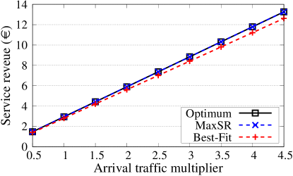
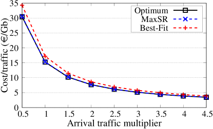
Impact of Physical Link latency and Arrival Traffic. Figure 2 shows the impact of the traffic arrival intensity on the service revenue and cost/traffic ratio. MaxSR matches the optimum, and Best-Fit performs close to the optimum in both service revenue and cost/traffic ratio. As it has no backtracking mechanism, Best-Fit does not serve a request whenever any of its VNFs cannot be served within its delay budget, i.e., it has no budget flexibility; therefore, it achieves lower service revenue than the optimum. While the cost of physical links increases proportionally to the traffic, the costs of VMs in turning-on mode remains constant, and their cost in active mode increases less than proportionally with the traffic; the resulting effect is that cost/traffic ratio decreases with the traffic – which conforms to the intuitive notion that serving larger amounts of traffic is more cost-efficient. Best-Fit incurs more cost compared to MaxSR and optimum because it does not support VNF migration, causing a VNF to continue running on a high-cost VM even if a low-cost VM becomes available. The excess VMs CPU cost and transmission cost scale with the traffic, whereas the excess VMs idle cost remains constant; therefore, the difference between Best-Fit and optimum becomes smaller as traffic increases.

(a)

(b)

Figure 3: Small-scale scenario. Impact of physical link latecy on absolute value of service revenue and cost/traffic ratio. Arrival traffic multiplier = $1$.

(a) Physical link delay = $3$ ms.

(b) Phsysical link delay = $7$ ms.

Figure 4: Fraction of deployed service requests for each service and algorithm. Arrival traffic multiplier = 1.

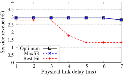
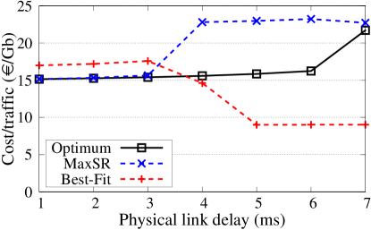
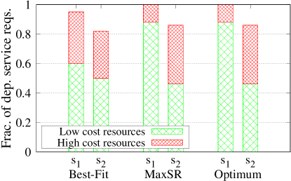
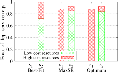
Figure 3 shows the impact of physical link latency on the service revenue and cost/traffic ratio. For all latency values, MaxSR is still able to achieve optimum service revenue. As shown in Figure 4a, no strategy (not even optimum) can serve all requests when the physical link delay is $3$ ms especially, for service $s_{2}$. The reason is that when the number of concurrent requests becomes more than two, both optimum and MaxSR give the priority to the high-revenue service $s_{1}$ and requests for $s_{2}$ will only be processed if resources are available. When the physical link delay increases, service requests need more computational capacity on VMs to meet their target delay, in order to offset longer network delays. Specifically, when the physical link delay is $7$ ms, requests of type $s_{1}$ can only be served on high-capacity VMs, and therefore, concurrent requests of this type can not be served. This is confirmed by the degradation of the optimum in Figure 3a, and in Figure 4b, where the fraction of served requests of type $s_{1}$ becomes less than $1$ when the physical link delay is $7$ ms.

Best-Fit gains substantially lower service revenue compared to others, especially for higher values of physical link delay. As shown in Figure 4b, this is due to the fact that Best-Fit cannot deploy requests of type $s_{1}$ in those cases. This, in turn, is due to the fact that it does not support backtracking: when the delay budget for the second VNF in the chain of $s_{1}$ is violated, no corrective action is taken and the whole request fails.

Figure 3b shows MaxSR has a higher cost/traffic ratio when the physical link delay is over $4$ ms. The reason is that the need for backtracking increases with the physical link delay, and VMs become more likely to be scaled to their maximum capacity, which results in a higher cost. As one might expect, the cost/traffic ratio for Best-Fit decreases when physical link delay $\geq 4$ ms because it does not serve requests of higher cost service $s_{1}$. Recall that the cost of a service depends on the amount of required CPU on VMs, and therefore services with lower target delays incur more costs to serve one unit of traffic.

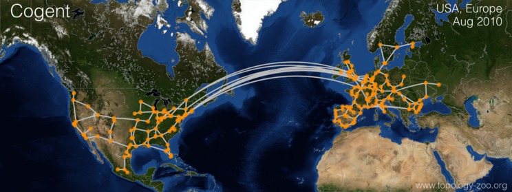
Large-scale scenario. We consider the real-world inter-datacenter network Cogent, a tier $1$ Internet service provider (Figure 5). This network topology contains $197$ access nodes with $245$ physical links and $32$ datacenters. We set the cost of links connecting the datacenters to $0.02$ €/GB. The delay of logical links connecting the datacenters is set to be proportional to their geographical lengths, while the links inside each datacenter are assumed to be ideal having no capacity limit, latency, and cost. We assume each datacenter hosts $42$ VMs, each of which is connected to some edge switches. We categorize VMs within each datacenter in small, medium, and large types according to their capacity and cost, as described in Table III. We assume VMs need one minute to setup before being active.

Figure 5: Cogent Network Topology.

We consider the four different services described in Table II, each of which is a representative of a category of real 5G applications. In this scenario, we assume that the VNFFG of each service is a chain of five VNFs. We further assume that the computational complexity, i.e., $\omega$ and maximum number of instances, i.e., $N(s,q)$ for two VNFs of service $s_{4}$ are three, while other VNFs have $\omega=1$ and $N(s,q)=1$. Similar to the previous scenario, we consider an equal number of requests for each service where requests arrive across time steps with the average inter-arrival time of three minutes and end after an average duration of two hours, and the total system lifespan is assumed to be one day. In this experiment, we set $H$ to $40$ minutes and $\tau$ to $20$ minutes.

(a)

(b)

Figure 6: Large-scale scenario. Impact of service requests arrival traffic on absolute value of service revenue and cost/traffic ratio. Physical link delay multiplier = $1$.

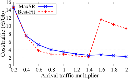
Impact of Physical Link latency and Arrival Traffic. As explained above, the optimum values cannot be obtained for this scenario in a reasonable time and therefore we rely on results for MaxSR and Best-Fit. Figure 6a shows the effect of arrival traffic on the service revenue, while Figure 7 shows the fraction of requests of each service that can be successfully deployed. We observe that service revenue for MaxSR changes almost proportionally with the traffic because increasing the traffic almost does not impact the fraction of served requests by this algorithm. Best-Fit serves a lower fraction of service requests, and therefore achieves lower revenue. Besides, Best-Fit shows a drop-off in service revenue when the arrival traffic multiplier is $1.6$: as confirmed by Figure 7b, this is because Best-Fit does not serve requests of high traffic service $s_{4}$ when the traffic multiplier is over $1.6$, due to its lack of support for multiple VNF instances.

(a) Traffic multiplier = $1.0$

(b) Traffic multiplier = $1.6$

Figure 7: Fraction of deployed service requests for each service and algorithm. Physical link delay multiplier = $1$.

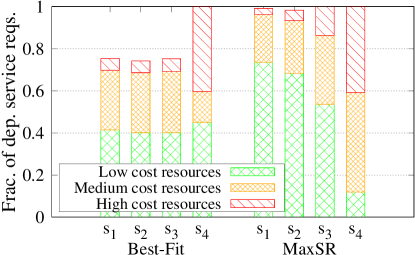
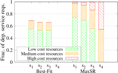
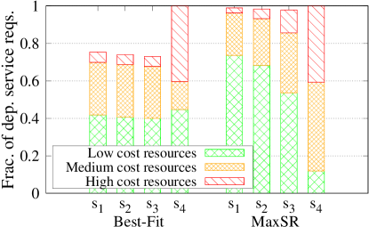
Figure 6b shows the impact of arrival traffic on the cost/traffic ratio. Best-Fit has lower cost/traffic ratio when arrival traffic multiplier is less than $1.4$, since MaxSR must use resources with higher cost and higher computational capabilities to serve more service requests; in other words, Best-Fit serves less traffic but that traffic is served cheaply. Similar to service revenue the values of cost/traffic ratio for Best-Fit have a significant rise when the arrival traffic multiplier is $1.6$, as confirmed by Figure 8, when the traffic multiplier increases from $1.0$ to $1.6$, Best-Fit is no longer able to serve a significant fraction of the total traffic. As shown by Figure 7, the traffic Best-Fit is unable to serve mainly belongs to the low cost service $s_{4}$, which results in a higher cost for served traffic.

(a) Traffic multiplier = $1.0$

(b) Traffic multiplier = $1.6$

Figure 8: Fraction of offered traffic deployed on each resource type for each algorithm. low, med, high and not dep. mean the fraction of offered traffic served on low cost resources, medium cost resources, high cost resources, and which is not served, respectively. Physical link delay multiplier = $1$.

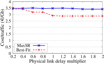
Figure 9a shows the impact of physical link latency on the service revenue. Similar to the small-scale scenario, MaxSR outperforms Best-Fit especially for higher values of physical link delays, because the latter cannot serve the requests for services with low target delay (hence, higher revenue). As these service types have higher cost, they will also cause the cost/traffic ratio for Best-Fit to be lower than MaxSR as shown in Figure 9b.

(a)

(b)

Figure 9: Large-scale scenario. Impact of physical link delay on absolute value of service revenue and cost/traffic ratio. Arrival traffic multiplier = 1.

(a) Physical link delay multiplier = $0.6$

(b) Physical link delay multiplier = $1.2$

Figure 10: Fraction of deployed service requests for each service and algorithm. Arrival traffic multiplier = $1$.

Running Time. We run our experiments using a server with $40$-core Intel Xeon E5-2690 v2 3.00GHz CPU and $64$ GB of memory. To compare the running time of different algorithms, we consider the case where the arrival traffic and physical link delay multipliers are equal to one. For each scenario, we run the algorithm $50$ times and report the average running time in Table IV. MaxSR and Best-Fit are substantially faster than brute-force in the small-scale scenario. The prohibitively long running time for brute-force highlights its poor scalability, and makes it inapplicable for the large-scale scenario in practice. The results for the large-scale scenario show that although MaxSR has higher running time compared to Best-Fit due to backtracking, both of them are scalable and adequately fast for large-scale networks.

TABLE IV: Running time (in seconds)

Scenario	Brute-force	MaxSR	Best-Fit
Small-scale	$399$	$0.2$	$0.14$
Large-scale	-	$21$	$2$

Sec. VI Conclusion

We proposed a dynamic service deployment strategy in 5G networks, accounting for real-world aspects such as VM setup times, and jointly making all the required decisions. We first formulated the problem of joint requests admission, VM activation, VNF placement, resource allocation, and traffic routing as a MILP based on the complete knowledge of requests arrival and departure times. We took the MNO profit as the main objective to be optimized over the entire system lifespan, leveraging a queueing model to ensure all requests adhere to their latency targets. Our model also accounted for the key features of 5G services such as complex VNF graphs and arbitrary input traffic.

Due to the problem complexity, we further proposed a heuristic, MaxSR, which has polynomial complexity and attains near-optimal solutions, while only needing the knowledge/prediction of the upcoming service requests in a short time horizon. The algorithm works in a sliding-horizon fashion, rearranging the current-served requests across existing VMs to reduce the deployment costs, and admitting the new ones as they arrive at the system. Furthermore, the parameters of MaxSR allow for different tradeoffs between solution optimality and running time. We demonstrated the effectiveness and efficiency of our approach through a numerical evaluation including different network scenarios.

References

- [1] ETSI. (2017) Network Functions Virtualisation (NFV); Management and Orchestration.
- [2] S. Agarwal, F. Malandrino, C. F. Chiasserini, and S. De, “Vnf placement and resource allocation for the support of vertical services in 5g networks,” IEEE/ACM Transactions on Networking, vol. 27, no. 1, pp. 433–446, Feb. 2019.
- [3] B. Yi, X. Wang, K. Li, M. Huang et al., “A comprehensive survey of network function virtualization,” Computer Networks, vol. 133, pp. 212–262, 2018.
- [4] R. Cohen, L. Lewin-Eytan, J. S. Naor, and D. Raz, “Near optimal placement of virtual network functions,” in IEEE Conference on Computer Communications (INFOCOM), Apr. 2015, pp. 1346–1354.
- [5] Lin Gu, Sheng Tao, Deze Zeng, and Hai Jin, “Communication cost efficient virtualized network function placement for big data processing,” in IEEE Conference on Computer Communications Workshops (INFOCOM WKSHPS), Apr. 2016, pp. 604–609.
- [6] M. Mechtri, C. Ghribi, and D. Zeghlache, “A scalable algorithm for the placement of service function chains,” IEEE Transactions on Network and Service Management, vol. 13, no. 3, pp. 533–546, Sep. 2016.
- [7] C. Pham, N. H. Tran, S. Ren, W. Saad, and C. S. Hong, “Traffic-aware and energy-efficient vnf placement for service chaining: Joint sampling and matching approach,” IEEE Transactions on Services Computing, pp. 1–1, 2017.
- [8] M. M. Tajiki, S. Salsano, L. Chiaraviglio, M. Shojafar, and B. Akbari, “Joint energy efficient and qos-aware path allocation and vnf placement for service function chaining,” IEEE Transactions on Network and Service Management, vol. 16, no. 1, pp. 374–388, Mar. 2019.
- [9] J. Pei, P. Hong, K. Xue, and D. Li, “Efficiently embedding service function chains with dynamic virtual network function placement in geo-distributed cloud system,” IEEE Transactions on Parallel and Distributed Systems, vol. 30, no. 10, pp. 2179–2192, Oct. 2019.
- [10] G. Sallam and B. Ji, “Joint placement and allocation of virtual network functions with budget and capacity constraints,” in IEEE Conference on Computer Communications (INFOCOM), Apr. 2019, pp. 523–531.
- [11] M. A. Tahmasbi Nejad, S. Parsaeefard, M. A. Maddah-Ali, T. Mahmoodi, and B. H. Khalaj, “vspace: Vnf simultaneous placement, admission control and embedding,” IEEE Journal on Selected Areas in Communications, vol. 36, no. 3, pp. 542–557, Mar. 2018.
- [12] R. Zhou, Z. Li, and C. Wu, “An efficient online placement scheme for cloud container clusters,” IEEE Journal on Selected Areas in Communications, vol. 37, no. 5, pp. 1046–1058, May 2019.
- [13] T. Kuo, B. Liou, K. C. Lin, and M. Tsai, “Deploying chains of virtual network functions: On the relation between link and server usage,” IEEE/ACM Transactions on Networking, vol. 26, no. 4, pp. 1562–1576, Aug. 2018.
- [14] X. Fei, F. Liu, H. Xu, and H. Jin, “Adaptive vnf scaling and flow routing with proactive demand prediction,” in IEEE Conference on Computer Communications (INFOCOM), Apr. 2018, pp. 486–494.
- [15] H. Tang, D. Zhou, and D. Chen, “Dynamic network function instance scaling based on traffic forecasting and vnf placement in operator data centers,” IEEE Transactions on Parallel and Distributed Systems, vol. 30, no. 3, pp. 530–543, Mar. 2019.
- [16] Y. Jia, C. Wu, Z. Li, F. Le, and A. Liu, “Online scaling of nfv service chains across geo-distributed datacenters,” IEEE/ACM Transactions on Networking, vol. 26, no. 2, pp. 699–710, Apr. 2018.
- [17] Y. Li, L. T. X. Phan, and B. T. Loo, “Network functions virtualization with soft real-time guarantees,” in IEEE Conference on Computer Communications (INFOCOM). IEEE, 2016, pp. 1–9.
- [18] V. Eramo, E. Miucci, M. Ammar, and F. G. Lavacca, “An approach for service function chain routing and virtual function network instance migration in network function virtualization architectures,” IEEE/ACM Transactions on Networking, vol. 25, no. 4, pp. 2008–2025, 2017.
- [19] J. Liu, W. Lu, F. Zhou, P. Lu, and Z. Zhu, “On dynamic service function chain deployment and readjustment,” IEEE Transactions on Network and Service Management, vol. 14, no. 3, pp. 543–553, Sep. 2017.
- [20] M. Huang, W. Liang, Y. Ma, and S. Guo, “Maximizing throughput of delay-sensitive nfv-enabled request admissions via virtualized network function placement,” IEEE Transactions on Cloud Computing, pp. 1–1, 2019.
- [21] F. Malandrino, C. F. Chiasserini, C. Casetti, G. Landi, and M. Capitani, “An optimization-enhanced mano for energy-efficient 5g networks,” IEEE/ACM Transactions on Networking, vol. 27, no. 4, pp. 1756–1769, Aug. 2019.
- [22] F. Malandrino, C.-F. Chiasserini, G. Einziger, and G. scalosub, “Reducing service deployment cost through vnf sharing,” IEEE/ACM Transactions on Networking, vol. PP, 10 2019.
- [23] Q. Zhang, F. Liu, and C. Zeng, “Adaptive interference-aware vnf placement for service-customized 5g network slices,” in IEEE Conference on Computer Communications (INFOCOM), Apr. 2019, pp. 2449–2457.
- [24] N. Alliance, “Description of network slicing concept,” NGMN 5G P, vol. 1, p. 1, 2016.
- [25] I. Dumitrescu and N. Boland, “Algorithms for the weight constrained shortest path problem,” International Transactions in Operational Research, vol. 8, no. 1, pp. 15–29, 2001.
- [26] D. Bega, M. Gramaglia, M. Fiore, A. Banchs, and X. Costa-Pérez, “Deepcog: Optimizing resource provisioning in network slicing with ai-based capacity forecasting,” IEEE Journal on Selected Areas in Communications, vol. 38, no. 2, pp. 361–376, 2020.