Planets Across Space and Time (PAST). I. Characterizing the Memberships of Galactic Components and Stellar Ages: Revisiting the Kinematic Methods and Applying to Planet Host Stars

Abstract

Over 4,000 exoplanets have been identified and thousands of candidates are to be confirmed. The relations between the characteristics of these planetary systems and the kinematics, Galactic components, and ages of their host stars have yet to be well explored. Aiming to addressing these questions, we conduct a research project, dubbed as PAST (Planets Across Space and Time). To do this, one of the key steps is to accurately characterize the planet host stars. In this paper, the Paper I of the PAST series, we revisit the kinematic method for classification of Galactic components and extend the applicable range of velocity ellipsoid from $\sim 100$ pc to $\sim 1,500$ pc from the sun in order to cover most known planet hosts. Furthermore, we revisit the Age-Velocity dispersion Relation (AVR), which allows us to derive kinematic age with a typical uncertainty of 10-20% for an ensemble of stars. Applying the above revised methods, we present a catalog of kinematic properties (i.e. Galactic positions, velocities, the relative membership probabilities among the thin disk, thick disk, Hercules stream, and the halo) as well as other basic stellar parameters for 2,174 host stars of 2,872 planets by combining data from Gaia, LAMOST, APOGEE, RAVE, and the NASA exoplanet archive. The revised kinematic method and AVR as well as the stellar catalog of kinematic properties and ages lay foundation for future studies on exoplanets from two dimensions of space and time in the Galactic context.

1 introduction

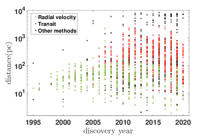
It has been a quarter century since the discovery of the first exoplanet. To date, over 4,000 exoplanets have been discovered and thousands of candidates are yet to be confirmed (NASA Exoplanet Archive, EA hereafter; Akeson et al., 2013). There is a clear trend (shown in Figure 1, data from http://exoplanet.eu) that our knowledge of exoplanets is expanding in the Galaxy. Before 2005, most known exoplanets were confined in the solar neighborhood with distance less than $\sim$ 100-200 pc. Now, the map of exoplanets is much wider with a large range of distance up to $\sim$ 10,000 pc. Therefore, people began to study exoplanets in the context of the Galaxy. For example, there were continuous discussions on how to define the Galactic habitable zone (Gonzalez et al., 2001; Lineweaver et al., 2004; Sundin, 2006; Gowanlock et al., 2011; Jiménez-Torres et al., 2013; Balbi & Tombesi, 2017; Stojković et al., 2019), researches on the Galactic distribution of planets as a function of distance/population (e.g., Zhu et al., 2017), and studies on whether planet occurrence rate depends on the Galactic velocity (e.g., McTier & Kipping, 2019; Bashi & Zucker, 2019).

One of fundamental questions in studying exoplanets in the Galactic context is: what are the differences in the properties of planetary systems at different positions in the Galaxy with different ages? The answer of this question will provide insights on the formation and evolution of the ubiquitous and diverse exoplanets in different Galactic environments. Aiming to addressing the question, in a series of papers from here on, we conduct statistical studies of planets at different positions in the Galaxy with different ages, a project that we dub as PAST (Planets Across Space and Time).

Figure 1: The distance of planet host stars to the Sun vs. the year of discovery. Planets discovered by different methods are plotted in different colours.

To this end, the first step is to figure out where the exoplanets are in the Galaxy. Specifically, for a given exoplanet host star, we would like to know which Galactic component (i.e., the thin disk, the thick disk or the halo) it belongs to. One of well-established methods to distinguish these Galactic components is the kinematic approach as different components generally have different kinematic characteristics. For example, the thin disk has a smaller vertical scale-height (Bovy et al., 2012a; Wu et al., 2018), but the thick disk is generally kinematically hotter with larger velocity dispersions (Gilmore et al., 1989; Reddy et al., 2003; Bensby et al., 2003, 2014; Buder et al., 2018). By comparing the kinematic properties of a given star to the typical kinematic characteristics of a Galacic component, one may calculate the likelihood that the star belongs to this component (e.g. Bensby et al., 2003). However, the kinematic characteristics of this method were obtained with data in the Solar neighborhood within $\sim$ 100 pc (Bensby et al., 2003, 2014), and thus limiting this kinematic method to a relatively small range of area. Thanks to the recent large scale star surveys both from space (e.g., Gaia, Gaia Collaboration et al., 2016, 2018a, 2018b) and ground (e.g., LAMOST, Wang et al., 1996; Su & Cui, 2004; Cui et al., 2012; Zhao et al., 2012; Luo et al., 2012), we are now allowed to extend the kinematic method to beyond 1,000 pc in order to characterize the majority of exoplanet host stars.

The second step is to obtain the ages of exoplanet host stars since most of exoplanet host stars have no (accurate) age estimates. Stellar ages can hardly be measured but only be inferred or estimated indirectly through a number of techniques, which have their own strength and weakness (Soderblom, 2010). For example, the widely-used isochrone placement method is applicable for estimating ages of a large range of stars, but it usually suffers from relatively large uncertainty ($\sim 50\%$ typically) for main sequence stars, which are the bulk of exoplanet hosts (e.g. Berger et al., 2020b). Asteroseismology is significantly better than any other age-dating method, which can deliver age estimates for individual stars with uncertainties of $\sim 10\%-20\%$ (e.g. Gai et al., 2011; Chaplin et al., 2014). However, this method requires observation with sufficiently accurate, high-cadence photometric measurements and it can only be applicable for stars with a limited range of spectral types that exhibit prominent oscillations. In addition, the carbon and nitrogen abundances have been suggested to be age indicators, but it is usually applicable for giant stars, and the reported age has achieved a precision of $\sim$ 20%-30% (Martig et al., 2016; Ness et al., 2016; Ho et al., 2017; Wu et al., 2018).

Stellar ages can also be estimated statistically from some empirical relationships. It has been known for decades that older stars have larger velocity dispersion, the so called Age-Velocity dispersion Relation (AVR) (Strömberg, 1946; Parenago, 1950; Wielen, 1977; Holmberg et al., 2009). To derive age from AVR, one generally just needs the stellar kinematics, and thus the age is also called kinematic age. Unlike the methods mentioned above, the kinematic method is only applicable to ensembles (not individual) of stars. Nevertheless, kinematic age is still meaningful from a statistical view given the fast rise of exoplanet population. Furthermore, the strength of kinematic age is that it uses only the 3D space motions (i.e., astrometry and radial velocities) without involving stellar evolutionary model, and thus it can apply to stars in a large range of various parameters (Soderblom, 2010). In recent years, the kinematic method has ushered in a major opportunity, thanks to the high-quality astrometry and radial velocity observations for millions of stars (including thousands of exoplanet hosts) provided mainly by the Gaia and LAMOST.

In this paper, we revisit the methods to characterize stellar kinematic properties and apply them to over 2,000 exoplanet host stars based on their astrometry and radial velocities provided mainly by Gaia and LAMOST. Specifically, in section 2, we revisit the kinematic method to identify Galactic components (e.g., thin/thick disk). In section 3, we revise the AVR to derive kinematic ages. Applying the revised kinematic method and AVR, in section 4, we present a catalog of kinematic properties for 2,174 planet host stars and conduct some analyses. In section 5, we discuss our results and some future prospects. In section 6, we provide some importing guidelines, cautions, and limitations to utilize the kinematic methods and planet host catalog. Finally, we summarize in section 7.

2 Revisiting the Kinematic Method to Classify the Galactic Components

In this section, we revisit the kinematic method to classify stars into different Galactic components (e.g., thin/thick disks). The key is revising the characteristic kinematic parameters (section 2.3), an extension from the solar neighborhood ($\sim 100$ pc) to $\sim 1,500$ pc in order to cover most planet hosts as shown in Figure 1.

2.1 Space Velocities and Galactic Orbits

We calculated the 3D Galactocentric cylindrical coordinates $(R,\theta,Z)$ by adopting a location of the Sun of $R_{\odot}$= 8.34 kpc (Reid et al., 2014) and $Z_{\odot}$ = 27 pc (Chen et al., 2001). The Galactic rectangular velocities relative to the Sun $(U,V,W)$ and their errors were calculated by the right-handed coordinate system based on the formulae and matrix equations presented in Johnson & Soderblom (1987). Here, $U$ is positive when pointing to the direction of the Galactic center, $V$ is positive along the direction of the Sun orbiting around the Galactic center, and $W$ is positive when pointing towards the North Galactic Pole. Cylindrical velocities $V_{R}$, $V_{\theta}$, and $V_{Z}$ are defined as positive with increasing $R$, $\theta$, and $Z$, with the latter towards the North Galactic Pole. To obtain the Galactic rectangular velocities relative to the local standard of rest (LSR) $(U_{\rm LSR},V_{\rm LSR},W_{\rm LSR})$, we adopted the solar peculiar motion [$U_{\odot}$, $V_{\odot}$, $W_{\odot}$] = [9.58, 10.52, 7.01] $\rm km\ s^{-1}$ (Tian et al., 2015).

2.2 Classification of Galactic Components

We adopted the widely-used kinematic approach as in Bensby et al. (2003, 2014) to classify the stars in our sample into different Galactic components, e.g., thin and thick disk stars. This method assumes that the Galactic velocities ($U_{\rm LSR},V_{\rm LSR},W_{\rm LSR}$) in different components (the thin disk, the thick disk, the halo, and the Hercules stream) follow a multi-dimensional Gaussian distribution as

$$f(U,V,W)=k\times{\rm exp}$$ (1)

$$\left(-\frac{(U_{\rm LSR}-U_{\rm asym})^{2}}{2{\sigma_{U}}^{2}}-\frac{(V_{\rm LSR}-V_{\rm asym})^{2}}{2{\sigma_{V}}^{2}}-\frac{W_{\rm LSR}^{2}}{2{\sigma_{W}}^{2}}\right),$$

where the normalization coefficient

$$k=\frac{1}{(2\pi)^{3/2}\sigma_{U}\sigma_{V}\sigma_{W}}.$$ (2)

Here, $\sigma_{U}$, $\sigma_{V}$, and $\sigma_{W}$ are the characteristic velocity dispersions, and $V_{\rm asym}$ and $U_{\rm asym}$ are the asymmetric drifts.

For $V_{\rm asym}$, following Binney & Tremaine (2008) we adopted

$$V_{\rm asym}=\bar{V_{\theta}}-V_{c},$$ (3)

where $V_{c}$ is the circular speed of LSR as 238 $\rm km\ s^{-1}$ (Schönrich, 2012) and $\bar{V_{\theta}}$ is the mean value of azimuthal velocities for a given component. For $U_{\rm asym}$, we adopted $U_{\rm asym}=0$ for the disk and halo components and $U_{\rm asym}=-40\rm km\ s^{-1}$ for Hercules stream component (Binney & Tremaine, 2008; Bensby et al., 2014).

The relative probabilities between two different components, i.e., the thick-disk-to-thin-disk $(TD/D)$, thick-disk to halo $(TD/H)$, the Hercules-to-thin-disk $(Herc/D)$, and the Hercules-to-thick-disk $(Herc/TD)$ can be calculated as

$$\frac{TD}{D} =\frac{X_{\rm TD}}{X_{\rm D}}\cdot\frac{f_{\rm TD}}{f_{\rm D}}, \quad\frac{TD}{H} =\frac{X_{\rm TD}}{X_{\rm H}}\cdot\frac{f_{\rm TD}}{f_{\rm H}},$$ (4)

$$\frac{Herc}{D} =\frac{X_{\rm Herc}}{X_{\rm D}}\cdot\frac{f_{\rm Herc}}{f_{\rm D}}, \quad\frac{Herc}{TD} =\frac{X_{\rm Herc}}{X_{\rm TD}}\cdot\frac{f_{\rm Herc}}{f_{\rm TD}},$$ (5)

where X is the fraction of stars for a given component.

Then for stars in our planet host sample, we calculated their above probabilities, and classified them into different Galactic components by adopting the same criteria as in Bensby et al. (2014), which are (1) thin disk: $TD/D<0.5\,\,\&\,\,Herc/D<0.5$, (2) thick disk: $TD/D>2\,\,\&\,\,TD/H>1\,\,\&\,\,Herc/TD<0.5$, (3) halo: $TD/D>2\,\,\&\,\,TD/H<1\,\,\&\,\,Herc/TD<0.5$, and (4) Hercules: $Herc/D>1\,\,\&\,\,Herc/TD>1$.

2.3 Revision of Characteristic Kinematic Parameters

One of the important steps during the above classification procedure is to obtain the characteristic kinematic parameters for each Galactic component, i.e., $\sigma_{U}$, $\sigma_{V}$, $\sigma_{W}$, $U_{\rm asym}$, $V_{\rm asym}$, and $X$. In the solar neighbourhood within $\sim 100$ pc from the Sun, these parameters are available from Bensby et al. (2014), which are list in Table 1 here. However, as shown in Figure 1, the stars in our sample are located in a much wider zone (up to several kpc from the Sun). It has been found that the velocity ellipsoids change with the Galactic position (Williams et al., 2013). Therefore, the values of these characteristic kinematic parameters for each component should be revised and extended (section 2.3) so that they are applicable for stars in a larger range of $Z$ (e.g., $|Z|<1.5$ kpc) and R ($7.5<R<10.0$ kpc).

Table 1: Characteristics for stellar components in the Solar neighbourhood from Bensby et al. (2014).^†

	$\sigma_{\rm U}$	$\sigma_{\rm V}$	$\sigma_{\rm W}$	$U_{\rm asym}$	$V_{\rm asym}$	$X$
	———–  [km s-1]  ———–
Thin disk	35	20	16	0	$-15$	0.85
Thick disk	67	38	35	0	$-46$	0.09
Halo	160	90	90	0	$-220$	0.0015
Hercules	26	9	17	$-40$	$-50$	0.06

2.3.1 calibration sample

To revise the values of characteristic kinematic parameters, we rely on a calibration sample based on the LAMOST and Gaia data. The LAMOST main-sequence turn-off and subgiant (MSTO-SG) star sample of (Xiang et al., 2017a) provides the estimates of stellar age, mass, and RV for 0.93 million Galactic-disk stars from the LAMOST Galactic spectroscopic surveys. The typical uncertainty in age is 34%.

To construct the calibration sample, we first cross-matched the above LAMOST MSTO-SG catalog with the Gaia DR2 catalog. This was done by using the X-match service of CDS. We set a critical distance of 1.25 arcseconds for position match. We carried out a magnitude cut, which was set as the G magnitude difference less than 2.3, to ensure our cross-matches were of similar brightness. The G magnitudes for the LAMOST MSTO-SG stars were calculated by using the $\rm XSTPS-GAC$ g, r, and i $\rm color-color$ polynomial fits in Table 7 of Jordi et al. (2010). For stars with multiple matches, we kept those with the smallest angular separations. After the above cross-match, we have 863,663 stars left.

We then applied the following filters to further clean the calibration sample.

(1) Binary filter. We removed binary star systems because their kinematics contain additional motions (Dehnen & Binney, 1998). This was done by choosing stars flagged as ’Normal star’ (i.e., single and with spectral type of AFGKM) in the LAMOST MSTO-SG catalog (Xiang et al., 2017a).

(2) Parallax precision filter. Following Dehnen & Binney (1998), we removed stars with relative parallax errors larger than 10 percent as reported in the Gaia DR2.

(3) Age precision filter. We removed stars with age older than 14 Gyr or the error of age larger than 25% or blue straggler stars ($|Z|>1.5$ kpc and age younger than 2 Gyr) in the LAMOST MSTO-SG catalog.

(4) Distance filter (similar to Binney et al., 1997). The majority of the remaining stars are brighter than G mag=16 where the parallax has a median error of 0.0649 mas. Recalling the above 10 percent parallax precision requirement, then it leads to a distance limit $\sim 1/(0.0649/0.1)=1.54$ kpc. We therefore removed stars with distance larger than this limit. Such a cut at 1.54 kpc also makes the distance distribution of the calibration sample closer to that of the planet host sample (Figure 13).

Figure 2: Top panel: Galactocentric radius ($R$) vs. height ($Z$) for the calibration sample. (8.34 kpc, 0.027 kpc) marks the position of Sun. Bottom panel: Galactocentric radius ($R$) vs. angle ($\theta$) for the calibration sample. (8.34 kpc, 0) marks the position of Sun.

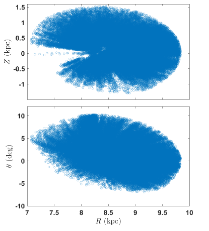
After applying the above filters, we are left with 130,403 stars. Figure 2 shows the location of stars in this calibration sample. As can be seen, these stars are mainly located at $7.5<R<10.0$ kpc and $|z|<1.5$ kpc, a region large enough to cover most known planet host stars (Figure 13).

Although most planet hosts are main-sequence stars while stars in the calibration sample are main-sequence turn-off stars and sub-giants, it should not affect the calibration of kinematic properties. In fact, it has been shown that the velocity ellipsoid (Binney et al., 2014; Büdenbender et al., 2015; Everall et al., 2019) and the AVR (Wielen, 1977; Holmberg et al., 2009; Yu & Liu, 2018; Mackereth et al., 2019) are independent on stellar evolution stage and effective temperature (mass). Therefore, the revised characteristic kinematic parameters (section 2.3) and AVR (section 3) from the calibration sample can be applicable for stars of different spectral types and evolutionary stages, including the planet host sample (section 4).

2.3.2 binning and examining the calibration sample

In order to calculate the characteristic kinematic parameters for each Galactic component as a function of ($R$, $Z$) in the Galaxy, we binned the calibration sample as follows. For $|Z|$, we set 8 bins with boundaries at $|Z|=$ 0, 0.1, 0.2, 0.3, 0.4, 0.55, 0.75, 1.0, and 1.5 kpc, resulting similar sizes ($\sim$ 20,000 stars) for all the bins except for the last two whose sizes are $\sim$ 10,000. For $R$, we set 5 bins with boundaries at $R=$ 7.5, 8.0, 8.5, 9.0, 9.5, and 10 kpc. In total, there are $5\times 8=40$ grids in the $R-Z$ space. Two of the grids ($R:9.5-10.0$ kpc, $|Z|:0.75-1.0\ \&\ 1.0-1.5$ kpc) have too few stars ($<400$) and thus are not considered hereafter.

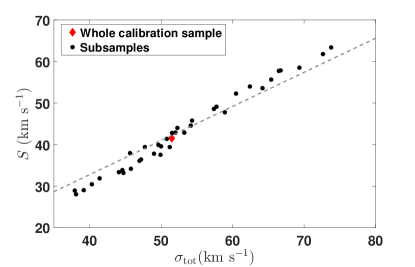
Following Binney et al. (2000), we examined the kinematically isotropic homogeneity in each bin of the calibration sample. The kinematical homogeneity requires that the dispersion in proper motions, $S$, follows

$$S=(\frac{2}{3}{\sigma_{\rm tot}}^{2})^{1/2}=[\frac{2}{3}(\sigma_{R}^{2}+\sigma_{\theta}^{2}+\sigma_{Z}^{2})]^{1/2}.$$ (6)

The result of this examination is shown in Figure 3. As can be seen, the calibration sample, either as a whole or as being divided into various grids, generally obeys the above relation, indicating the sample is kinematically unbiased.

Figure 3: The dispersion in proper motions, $S$, of the calibration sample as a function of the total dispersion in velocity, $\sigma_{\rm tot}$. The black dashed line represents where $S$ and $\sigma_{\rm tot}$ obey Equation 6.

2.3.3 classifying the calibration sample

Next, we classify stars in the calibration sample into different Galactic components. Following Bonaca et al. (2017), we identify halo stars if $V_{\rm tot}=(U_{\rm LSR}^{2}+V_{\rm LSR}^{2}+W_{\rm LSR}^{2})^{1/2}>220\ \rm km\ s^{-1}$. Stars with $V_{\rm LSR}\approx-50\ \pm\ 9\ \rm km\ s^{-1}$ and $(U_{\rm LSR}^{2}+W_{\rm LSR}^{2})^{(1/2)}\approx\rm 50-70\ km\ s^{-1}$ are selected as the Hercules stream (Famaey et al., 2005; Bensby et al., 2007, 2014). We adopt the age-defined thin and thick disc components with a boundary at 8 Gyr (Fuhrmann, 1998; Hou et al., 2013) to classify the rest sample into thin and thick disc stars. In Figure 4, we plot the Toomre diagram for the calibration sample. As expected, most stars with low velocities ($V_{\rm tot}\lesssim 50\rm km\ s^{-1}$) are in thin disk, while those with moderate velocities ($V_{\rm tot}\sim 70-180\ \rm km\ s^{-1}$) are mainly in thick disk (e.g. Feltzing et al. (2003); Adibekyan et al. (2013); Bensby et al. (2014). ).

Figure 4: The Toomre diagram of the calibration sample for different Galactic components. The diagram is colour-coded to represent different components. Dashed lines show constant values of the total Galactic velocity $V_{\rm tot}=100,\ 200,{\ \rm and}\ 300\ \rm km\ s^{-1}$.

Figure 5: The velocity dispersions as functions of position (R, Z) in the Galaxy for the calibration sample. The black line in each panel denotes the result of the best fit of Equation 7 using the coefficients in Table 2.

2.3.4 revising the velocity ellipsoid

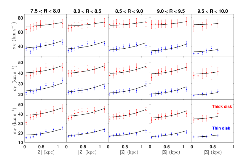
We then revise the velocity ellipsoid of each Galactic component, namely calculate $\sigma_{U}$, $\sigma_{V}$, $\sigma_{W}$, and $V_{\rm asym}$ of each grid in the $R-Z$ plane. Here, we revise those values only for the thin and thick disk components. For the halo and Hercules components, their numbers in each grid are too low for the revision, thus we adopt the velocity ellipsoid values as in Bensby et al. (2007, 2014) instead. The calculated values of $\sigma_{U}$, $\sigma_{V}$, $\sigma_{W}$, and $V_{\rm asym}$ for the thin and thick disk components are tabulated in Table 9 and visualized in Figure 5 and Figure 6.

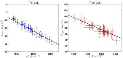
For velocity dispersion, according to Williams et al. (2013), it generally follows a simple formula:

$$\sigma=b_{1}+b_{2}\times\frac{R}{\rm kpc}+b_{3}\times(\frac{Z}{\rm kpc})^{2}{\rm km\ s^{-1}}.$$ (7)

We therefore fit $\sigma_{U}$, $\sigma_{V}$, $\sigma_{W}$ in this formula. To obtain the uncertainty of each fitting parameter, we assumed that the Galactic velocity following the Gaussian distribution $N(V,err\_V)$, where $err$ represents the corresponding uncertainty. Then, we resampled Galactic velocities based on these Gaussian distributions. After that, we refit the resampled data in the formula of Equation 7. We repeated the above resampling process 1,000 times and obtained 1,000 sets of best fits. The uncertainties (one-sigma interval) of the fitting parameters are set as the range of $50\pm 34.1$ percentiles of these 1,000 sets of best fits. Figure 5 shows the velocity dispersions ($\sigma_{U}$, $\sigma_{V}$, $\sigma_{W}$) as a function of $Z$ in each $R$ bin. The best fits are over-plotted as the black solid curves. The values of fitting parameters and their one-sigma uncertainties are summarized in Table 2. As expected, velocity dispersions generally increase with $Z$ for both thin and thick disks in all the $R$ bins.

Table 2: Fitting parameters of the velocity dispersion as functions of $(R,\ Z)$, i.e. Equation 7.

	$b_{1}$	$b_{2}$	$b_{3}$
$\sigma^{\rm D}_{U}$	$63.4^{+1.3}_{-3.2}$	$-3.2^{+0.3}_{-0.2}$	$7.6^{+0.5}_{-1.3}$
$\sigma^{\rm D}_{V}$	$41.6^{+0.7}_{-2.3}$	$-2.3^{+0.3}_{-0.1}$	$5.6^{+0.2}_{-0.9}$
$\sigma^{\rm D}_{W}$	$27.3^{+1.3}_{-1.5}$	$-1.2^{+0.2}_{-0.1}$	$5.0^{+0.2}_{-0.7}$
$\sigma^{\rm TD}_{U}$	$58.4^{+6.7}_{-4.4}$	$1.2^{+0.6}_{-0.7}$	$4.1^{+0.4}_{-0.8}$
$\sigma^{\rm TD}_{V}$	$44.9^{+5.3}_{-2.7}$	$-0.7^{+0.4}_{-0.5}$	$5.2^{+0.3}_{-1.0}$
$\sigma^{\rm TD}_{W}$	$55.8^{+1.8}_{-3.1}$	$-2.2^{+0.4}_{-0.2}$	$6.1^{+0.4}_{-1.0}$

For asymmetric velocity, according to Robin et al. (2003); Binney & Tremaine (2008), it generally follows the relation $V_{\rm asym}=-\frac{\sigma_{U}^{2}}{2V_{\rm LSR}}\left[\frac{\partial\ln\rho}{\partial\ln R}+\frac{\partial\ln\sigma_{U}^{2}}{\partial\ln R}+\left(1-\frac{\sigma_{V}^{2}}{\sigma_{U}^{2}}\right)+\left(1-\frac{\sigma_{W}^{2}}{\sigma_{U}^{2}}\right)\right]$. Therefore, we use the following formula to calculate $V_{\rm asym}$, i.e.,

$$V_{\rm asym}=\sigma_{U}^{2}/C_{0}.$$ (8)

Figure 6 shows $V_{\rm asym}$ as a function of $\sigma_{U}^{2}$. The best fits are over-plotted as the black solid lines. The values of $C_{0}$ are $-88.5^{+1.7}_{-1.9}\ \rm km\ s^{-1}$ and $-92.5^{+2.3}_{-2.1}\ \rm km\ s^{-1}$ for the thin and thick disks respectively, which are generally consistent with the theoretical estimate ($-82\pm 6\ \rm km\ s^{-1}$) (Binney & Tremaine, 2008).

Figure 6: The asymmetric velocity, $V_{\rm asym}$ as a function of $\sigma_{U}^{2}$ for the thin disk (left panel) and thick disk (right pannel). The black lines denote the results of the best fit using Equation 8.

2.3.5 revising the $X$ factor

Figure 7: The normalisation fraction $X$ of stars for each component as a function of Galactic radius $R$ and absolute value of height $|Z|$. The different colours denote subsamples of stars with different Galactic radii.

As defined in Equation 2.2, $X$ is the fraction of stars for a given component. For halo and Hercules stream, their number density distributions and structures are not quite clear yet. Thus, we set their $X$ as the observed fractions, i.e.,

$$X_{\rm H}=\frac{N_{\rm H}}{N_{\rm tot}},\ X_{\rm Herc}=\frac{N_{\rm Herc}}{N_{\rm tot}},$$ (9)

where $N_{\rm H}$, $N_{\rm Herc}$ and $N_{\rm tot}$ are the numbers of Hercules stream stars, halo stars, and total stars in each $(R-Z)$ grid.

For thin and thick disks, the number density is modeled as the following formula (Chen et al., 2001; Binney & Tremaine, 2008):

$$n(R,Z)=n^{0}\times{\rm exp}(-\frac{R-R_{\odot}}{h_{R}}){\rm exp}(-\frac{|Z|}{h_{Z}}),$$ (10)

where $h_{Z}$ and $h_{R}$ are the scale height and scale length of the disk, respectively. Here we take ($h_{R}$, $h_{z}$) as (3.4, 0.3) kpc for the thin disk and (1.8, 1.0) kpc for the thick disk (Binney & Tremaine, 2008; Cheng et al., 2012; Bovy et al., 2016). Then, the ratio of thick/thin disk star numbers in each $R-Z$ grid can be calculated as

$$X_{\rm TD/D}=X_{\rm TD}/X_{\rm D}=\frac{\int_{R}\int_{Z}{n_{\rm TD}(R,Z)}2\pi R{\rm d}R{\rm d}Z}{\int_{R}\int_{Z}{n_{\rm D}(R,Z)}2\pi R{\rm d}R{\rm d}Z}.$$ (11)

In practice, we first calculated nominal ratio, i.e., ${n^{0}}_{\rm TD}/{n^{0}}_{\rm D}$=0.098 (first term of the right-hand side of Equation 10) by solving Equation 11 with $X_{\rm TD}/X_{\rm D}=0.09/0.85$ for the solar neighbourhood ($((R-R_{\odot})^{2}+Z^{2})^{1/2}=100$ pc, Bensby et al. (2014)). Then, we applied this nominal ratio to Equation 11 to calculate the ratio of thick/thin disk star numbers in each $R-Z$ grid.

Finally, the $X$ of thin and thick disks were calculated as:

$$X_{\rm D}=(1-X_{\rm H}-X_{\rm Herc})\times\frac{1}{1+X_{\rm TD/D}},$$ (12)

$$X_{\rm TD}=(1-X_{\rm H}-X_{\rm Herc})\times\frac{X_{TD/D}}{1+X_{\rm TD/D}}.$$

The results of these revised $X$ values in all the $R-Z$ grids are tabulated in Table 9. Figure 7 shows the X values of various Galactic components as functions of Galactic radius $R$ and absolute value of height, $|Z|$. As expected, $X_{\rm D}$ ($X_{\rm TD}$) generally decrease (increase) with $|Z|$ in all the $R$ bins.

2.3.6 comparison to Bensby et al. (2014)

So far, we have calculated the characteristic parameters (i.e., $\sigma_{U}$, $\sigma_{V}$, $\sigma_{W}$, $U_{\rm asym}$, and $V_{\rm asym}$) as functions of $R$ and $Z$ (Table 9). In Table 3, we then compare our results in the solar neighbourhood (here bin with $R:8.0-8.5$ kpc and $|Z|<0.1$ kpc) to those of Bensby et al. (2014). As can be seen, both our results and those of Bensby et al. (2014) provide very similar values on these characteristic parameters, demonstrating that our revision (section 2) can also be reduced to the solar neighbourhood.

Table 3: The kinematic characteristics for stellar components in the Solar neighbourhood from Bensby et al. (2014) and this work.

	$X_{\rm D}$	$X_{\rm TD}$	$X_{\rm H}$	$X_{\rm Herc}$
Bensby et al. (2014)	0.85	0.09	0.0015	0.06
This work	0.84	0.10	0.0013	0.06
	$\sigma_{\rm U\_D}$	$\sigma_{\rm V\_D}$	$\sigma_{\rm W\_D}$	$V_{\rm asymD}$
Bensby et al. (2014)	35	20	16	-15
This work	34	21	16	-14
	$\sigma_{\rm U\_TD}$	$\sigma_{\rm V\_TD}$	$\sigma_{\rm W\_TD}$	$V_{\rm asymTD}$
Bensby et al. (2014)	67	38	35	-46
This work	65	39	35	-44

3 Revisiting the Age-Velocity Dispersion Relation to Derive Kinematic Ages

When the stars in the solar neighbourhood are binned by age, the velocity dispersion of each bin increases with its age. This age velocity relation (AVR) has been known and studied for decades (Strömberg, 1946; Parenago, 1950; Wielen, 1977; Holmberg et al., 2009). Similar relationship has also been inferred for external Galactic disk (Aumer et al., 2016; Robin et al., 2017). Here, we revisit the AVR with the calibration sample constructed in section 2.3.1.

3.1 Fitting AVR

In our study, we divided the foregoing calibration sample (section 2.3.1) into 30 bins with approximately equal sizes ($\sim$ 4,350 stars in each bins) according to their ages. Then we calculated the total velocity dispersion for each bin, i.e.,

$$\sigma_{\rm tot}=(\sigma_{U}^{2}+\sigma_{V}^{2}+\sigma_{W}^{2})^{\frac{1}{2}}.$$ (13)

Figure 8 shows the velocity dispersion as a function of the median age of each bin. As can be seen, all the components of velocity dispersion ($U_{\rm LSR},V_{\rm LSR},W_{\rm LSR}$) and the total velocity dispersion ($V_{\rm tot}$) increase with age. Following Holmberg et al. (2009); Aumer et al. (2016), we fit the AVRs shown in Figure 8 by using a simple power law formula, i.e.,

$$\sigma=k\times\left(\frac{t}{\rm Gyr}\right)^{\beta}\,\rm km\ s^{-1},$$ (14)

where t is stellar age, $\sigma$ is the velocity dispersion, $k$ and $\beta$ are two fitting parameters.

We used the Levenberg-Marquardt algorithm (LMA) to find the best fit. To obtain the uncertainty of each fitting parameter, we assumed that the Galactic velocity and age follows the Gaussian distribution $N(V,err\_V)$ and $N(t,err\_t)$, where $err$ represents the corresponding uncertainty. Then, we resampled Galactic velocities and stellar ages based on these Gaussian distributions. After that, we refit the AVR by using the resampled data. We repeated the above resampling process 1,000 times and obtained 1,000 sets of best fits. The uncertainties (one-sigma interval) of the fitting parameters are set as the range of $50\pm 34.1$ percentiles of these 1000 sets of best fits.

The values of the fitting parameters on the AVR are summarized in Table 4. We obtained $\beta$=$0.34^{+0.02}_{-0.01}$, $0.43^{+0.02}_{-0.02}$, $0.54^{+0.02}_{-0.02}$, and $0.40^{+0.02}_{-0.02}$, for $U_{\rm LSR},V_{\rm LSR},W_{\rm LSR}$, and $V_{\rm tot}$, respectively, which are consistent with the values derived from previous studies (Holmberg et al., 2009; Aumer & Binney, 2009, see section 3.5 for detail comparisons).

Figure 8: The Velocity dispersions for $U_{\rm LSR},V_{\rm LSR},W_{\rm LSR}$ and $V_{\rm tot}$ vs. age for the selected calibration star sample. The 30 bins have approximately equal numbers of stars ($\sim 4350$ in each); The solid black lines denote the respective best fit of refitting AVR (Equation 14) using the coefficients in Table 4.

Table 4: Fitting parameters of the Age-Velocity dispersion Relation (AVR, Equation 14).

	———  $U$  ———		———  $V$  ———		———  $W$  ———		———  $V_{\rm tot}$  ———
	$k$	$\beta$	$k$	$\beta$	$k$	$\beta$	$k$	$\beta$
section 3.1: AVR of the whole calibration sample
Whole sample	$23.66^{+0.66}_{-0.59}$	$0.34^{+0.02}_{-0.01}$	$12.49^{+0.49}_{-0.44}$	$0.43^{+0.02}_{-0.02}$	$8.50^{+0.47}_{-0.41}$	$0.54^{+0.02}_{-0.02}$	$27.55^{+0.82}_{-0.71}$	$0.40^{+0.02}_{-0.02}$
section 3.3: AVR of different radii
$R:7.5-8.0$ kpc	$24.16^{+0.17}_{-0.12}$	$0.33^{+0.01}_{-0.01}$	$14.32^{+0.10}_{-0.10}$	$0.39^{+0.01}_{-0.01}$	$8.74^{+0.08}_{-0.07}$	$0.57^{+0.01}_{-0.01}$	$30.90^{+0.16}_{-0.12}$	$0.36^{+0.01}_{-0.01}$
$R:8.0-8.5$ kpc	$25.31^{+0.15}_{-0.09}$	$0.33^{+0.01}_{-0.01}$	$14.18^{+0.06}_{-0.06}$	$0.39^{+0.01}_{-0.01}$	$8.84^{+0.07}_{-0.06}$	$0.54^{+0.02}_{-0.02}$	$29.91^{+0.07}_{-0.10}$	$0.38^{+0.01}_{-0.01}$
$R:8.5-9.0$ kpc	$23.40^{+0.13}_{-0.15}$	$0.34^{+0.01}_{-0.01}$	$11.84^{+0.03}_{-0.03}$	$0.46^{+0.01}_{-0.01}$	$8.30^{+0.05}_{-0.04}$	$0.55^{+0.01}_{-0.01}$	$27.05^{+0.20}_{-0.11}$	$0.40^{+0.005}_{-0.003}$
$R:9.0-9.5$ kpc	$22.28^{+0.09}_{-0.10}$	$0.35^{+0.02}_{-0.01}$	$12.27^{+0.04}_{-0.05}$	$0.42^{+0.01}_{-0.01}$	$8.32^{+0.05}_{-0.05}$	$0.54^{+0.02}_{-0.02}$	$26.42^{+0.11}_{-0.10}$	$0.40^{+0.02}_{-0.01}$
$R:9.5-10.0$ kpc	$22.73^{+0.22}_{-0.25}$	$0.32^{+0.03}_{-0.03}$	$12.66^{+0.15}_{-0.15}$	$0.44^{+0.04}_{-0.04}$	$8.27^{+0.08}_{-0.08}$	$0.53^{+0.04}_{-0.04}$	$27.74^{+0.18}_{-0.21}$	$0.38^{+0.02}_{-0.02}$
section 3.4: AVR of $|Z|<0.1$ kpc
$|Z|<0.1$ kpc	$23.15^{+0.61}_{-0.45}$	$0.33^{+0.01}_{-0.01}$	$12.43^{+0.41}_{-0.40}$	$0.42^{+0.01}_{-0.02}$	$7.98^{+0.40}_{-0.36}$	$0.56^{+0.02}_{-0.02}$	$27.01^{+0.68}_{-0.59}$	$0.39^{+0.02}_{-0.01}$
AVR of Holmberg et al. (2009)1
Holmberg et al. (2009)	$22.36^{+2.45}_{-2.08}$	$0.39^{+0.07}_{-0.09}$	$12.14^{+1.25}_{-1.04}$	$0.40^{+0.06}_{-0.05}$	$8.35^{+1.22}_{-1.03}$	$0.53^{+0.08}_{-0.05}$	$25.62^{+2.80}_{-2.68}$	$0.40^{+0.07}_{-0.05}$

3.2 AVRs of Different Galactic Components

Our calibration sample consists of 98,486 (75.51%) thin disk stars 23,572 (18.08%) thick disk stars, 8,152 (6.25%) Hercules stars, and 193 (0.15%) halo stars. To explore the difference of AVRs between different Galactic components, for each component, we divided stars into bins with approximately equal size according to their ages. Due to sample size, the bin numbers are set as 20, 10, 10, and 5 for thin disk, thick disk, Hercules stream, and halo respectively. For each component, we performed the same method as in section 3.1 to obtain the AVR.

Figure 9 displays the AVRs of different components. As can be seen, the AVRs obtained from the thin and thick disk components fit well to the power-law AVR derived from the whole calibration sample. For the Hercules stream, the dispersion of velocity component $\sigma_{W}$ generally follows the power-law AVR, but other components, i.e, $\sigma_{U}$ and $\sigma_{V}$ seem to be irrelevant with age. For the halo, the velocity dispersions are much larger than those predicted by the power-law AVR, and there is no clear trend between velocity dispersions and ages. Therefore, we conclude that the power-law AVR can only apply to the thin/thick disk components.

Figure 9: The AVRs of differnt Galactic components. The different colours denote subsamples of stars with different components. The black lines represents the best fit of AVR obtained from the whole sample.

3.3 Radial Variation of AVR

To explore how the AVR varies with Galactic radius, we divided the foregoing calibration sample (section 2.3.1) into to five subsamples according to their Galactic radii, i.e., $R=7.5-8.0$ kpc, $R=8.0-8.5$ kpc, $R=8.5-9.0$ kpc, $R=9.0-9.5$ kpc, and $R=9.5-10$ kpc. For each subsample, we performed the same method as in section 3.1 to fit the AVR. Figure 10 shows the fitted AVRs for the five subsamples. The fitting parameters of the five AVRs are summarized in Table 4. As can be seen, the AVRs are generally lower with the increase of $R$, which is caused by the decrease of velocity dispersion with $R$ (Equation 7). Therefore, the typical uncertainties in $k$, $\beta$ of AVRs obtained from the whole sample are generally larger than the five subsamples due to the radial variation. However, the values of $k$ and $\beta$ differ mildly with R (mean value: $\sim$ 5% for $k$ and 4% for $\beta$). As can be seen in Figure 10, the AVRs for the five subsamples are generally within $1-\sigma$ range of that for the whole sample (grey regions). This is consistent with the result derived from simulations in Aumer et al. (2016), which showed that the shape of the AVR is almost independent of $R$ when $R\gtrsim 6\rm kpc$.

Figure 10: The radial variation of AVRs. The different colours denote subsamples of stars with different Galactic radii. The grey region represents the $1-\sigma$ range of AVR obtained from the whole sample.

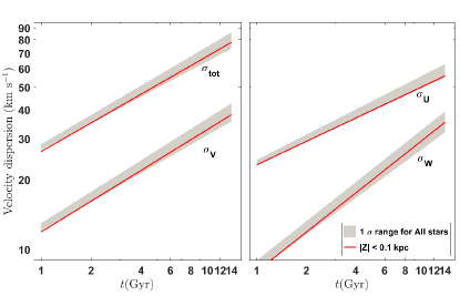
3.4 Vertical Selection Effect of AVR

Selecting stars from a limited vertical volume introduces phase correlations between stars which influence the values of velocity dispersions at the time of selection and before (Aumer et al., 2016). For example, when stars are selected close to $Z=0$, they are all close to their maxima in $|W_{\rm LSR}|$. Tracking them back in time, their vertical velocity dispersions thus have to be lower than at the time of selection (Aumer & Schönrich, 2015). To explore the vertical selection effect in our sample, following the method in Aumer et al. (2016), we compared the AVRs for stars with $|Z|<100$ pc and for all stars irrespective of the $Z$ position. The result is displayed in Figure 11. As can be seen, there is no significant difference between the AVR for $|Z|<100$ pc (red) and that for all stars (grey region). We conducted KS test between the velocity dispersions of stars with $|Z|<100$ pc and those of all stars. The p-values are 0.86, 0.97, 0.99, and 0.94 for $U_{\rm LSR},V_{\rm LSR},W_{\rm LSR}$, and $V_{\rm tot}$, respectively. Such high p-value values demonstrate the vertical selection effect has little influence in AVR.

Figure 11: Effect of vertical selection on velocity dispersions. The velocity dispersions are plotted as the solid red line for $|z|<100$ pc. The grey region represents the $1-\sigma$ range of AVR obtained from the whole sample.

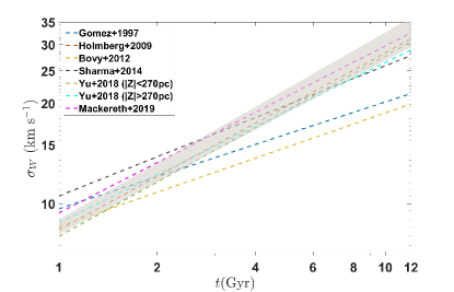
3.5 Comparison to Previous Works

Here, we compare our fitted AVR (section 3.1) to those AVRs fitted with different samples in previous studies. The result is plotted in Figure 12. As can be seen, our result is in good agreement with those of Holmberg et al. (2009); Yu & Liu (2018); Mackereth et al. (2019). Nevertheless, we note that our result differs significantly from those of Binney et al. (1997); Bovy et al. (2012b), and Sharma et al. (2014) on the younger and older ends, respectively.

All these studies fit their AVRs with different stellar samples. Gomez et al. (1997) used 2,812 stars from the Hipparcos data. Holmberg et al. (2009) used 2,640 FG main-sequence stars from the Geneva-Copenhagen Survey (GCS) data. Bovy et al. (2012b) used 3,365 stars from the APOGEE data. Sharma et al. (2014) used 5,201 stars from the GCS and RAVE data. Yu & Liu (2018) used 3,564 sub-giant/red giant stars from the LAMOST-Gaia data. Mackereth et al. (2019) used 65,719 stars from the APOGEE and Gaia data.

Our study used 130,403 stars which were selected from the LAMOST DR4 value added catalog with well constrained kinematics and ages (section 2.3.1). Due to the upgrade of sample size as well as the quality of star characterizations, the uncertainties of the AVR parameters have been largely reduced in this work. To better demonstrate this point, we performed a more detail comparison to the AVR of Holmberg et al. (2009), which are widely used and very close to our best fit of the AVR (Figure 12). We adopted the same procedures (section 3.1) to obtain the uncertainties of AVR but using the data of Holmberg et al. (2009). The results are summarized at the bottom part of Table 5. As can be seen, the typical errors in $k$ and $\beta$ decrease from $\sim 1-3\,\rm km\ s^{-1}$ and $0.05-0.08$ to $\sim 0.5\,\rm km\ s^{-1}$ and $0.02$, respectively. The reduction of uncertainties in AVR parameters leads to significant improvement in the precision of kinematic age (section 3.6).

Figure 12: The vertical AVRs from different studies. The dashed lines present results from previous studies. The grey region denotes the $1-\sigma$ range of the best fit obtained from our calibration sample.

3.6 Kinematic Age and Uncertainty

For a group of stars, the typical kinematic age can be derived by using the AVR (solving the Equation 14), which gives

$$t=\left(\frac{\sigma}{k\rm\,km\ s^{-1}}\right)^{\frac{1}{\beta}}\,\rm Gyr,$$ (15)

By means of error propagation, the relative uncertainty of kinematic age can be estimated as :

$$\frac{\Delta t}{t} =\sqrt{{(\frac{\partial\ln{t}}{\partial\beta}\Delta\beta)}^{2}+{(\frac{\partial\ln{t}}{\partial k}\Delta k)}^{2}+{(\frac{\partial\ln{t}}{\partial\sigma}\Delta\sigma)}^{2}}$$ (16)

$$=\sqrt{{\left(\ln\frac{t}{\rm Gyr}\right)^{2}\left(\frac{\Delta\beta}{\beta}\right)^{2}+\frac{1}{\beta^{2}}\left(\frac{\Delta k}{k}\right)^{2}+\frac{1}{\beta^{2}}\left(\frac{\Delta\sigma}{\sigma}\right)^{2}}},$$

where $\Delta$ represents the absolute uncertainty. For the sake of simplicity, here we assume $k$, $\beta$, and $\sigma$ are independent of each other. In other word, we neglect the covariances between them. It can be seen from the formula: the first term (due to the uncertainty of $\beta$) has positive correlation with the age ($t$), while the latter two terms are independent with age. Therefore, the relative uncertainty in age generally increases with age itself. For this reason, we set t=1 Gyr and t=10 Gyr to estimate the range of the relative uncertainty of age.

Based on Equation 16, we analyzed the budget of kinematic age uncertainty derived from AVR. The results are listed in the left part of Table 5. The uncertainties in AVR fitting parameters, i.e., $\Delta k$ and $\Delta\beta$, were calculated as the half width of the 1-sigma interval of $k$ and $\beta$ as listed in Table 4. The relative uncertainties in velocity dispersions ($\Delta\sigma/\sigma$) were adopted as the median relative uncertainties of velocity dispersions in our planet host stellar sample, which are 2.0%, 3.5%, 4.1%, and 2.4% for $\sigma_{U},\ \sigma_{V},\ \sigma_{W}$ and $\sigma_{\rm tot}$, respectively. Putting all the above uncertainties into Equation 16, we obtained the relative age uncertainties $\Delta t/t\sim 9.7-14.1\%$, $\Delta t/t\sim 11.8-20.1\%$, $\Delta t/t\sim 12.3-16.9\%$, and $\Delta t/t\sim 9.2-16.0\%$ for $\sigma_{U},\ \sigma_{V},\ \sigma_{W}$, and $\sigma_{\rm tot}$, respectively. The lower and upper values are calculated by assuming $t=1$ Gyr and $t=10$ Gyr respectively in Equation 16.

For comparison, we repeated the above budget calculation but using AVR of Holmberg et al. (2009, see the bottom part of Table 4). The results are listed in the right part of Table 5. As can be seen, for AVR from Holmberg et al. (2009), the uncertainties of $k$, $\beta$ are much larger and thus dominant, leading to a much larger (by a factor of $\sim 3$) uncertainty in the derived kinematic age.

As discussed in section 3.2, AVRs are not significant for halo and Hercules stream, therefore we suggest that this method to obtain kinematic age is only suitable for stars belonging to the Galactic disk components.

Table 5: The typical relative uncertainties of parameters and kinematic ages derived by the Age-Velocity Relations using data from Holmberg et al. (2009) and this work.

		This work	Holmberg et al. 2009
$U$	$\Delta k/k$	2.6%	10.1%
	$\Delta\beta/\beta$	4.4%	20.5%
	$\Delta\sigma/\sigma$	2.0%	2.0%
	$\Delta t/t$	$9.7\%-14.1\%$	$31.6\%-64.1\%$
$V$	$\Delta k/k$	3.7%	9.4%
	$\Delta\beta/\beta$	4.1%	13.8%
	$\Delta\sigma/\sigma$	3.5%	3.5%
	$\Delta t/t$	$11.8\%-20.1\%$	$23.32\%-44.4\%$
$W$	$\Delta k/k$	5.2%	14.1%
	$\Delta\beta/\beta$	3.7%	12.3%
	$\Delta\sigma/\sigma$	4.1%	4.1%
	$\Delta t/t$	$12.3\%-16.9\%$	$27.2\%-45.3\%$
$V_{\rm tot}$	$\Delta k/k$	2.8%	10.7%
	$\Delta\beta/\beta$	5.0%	15.0%
	$\Delta\sigma/\sigma$	2.4%	2.4%
	$\Delta t/t$	$9.2\%-16\%$	$27.4\%-54.1\%$

4 Application to Planet Host Stars

In this section, we apply the above revised kinematic method (section 2) and AVR (section 3) to a sample of planet host stars (section 4.1), providing a catalog of their kinematic properties (section 4.2), with focus on the Galactic components (section 4.3) and kinematic ages (section 4.4).

4.1 Data samples

This subsection describes how we constructed the planet host sample for further kinematic characterizing.

4.1.1 initializing planet host sample from EA

We initialized our planet host sample with the confirmed planets table and the Kepler DR 25 catalog from EA. The Kepler catalog contains 8,054 Kepler Objects of Interest (KOIs) in DR25. Here, we excluded KOIs flagged by ‘False Positive’ (FAP, Thompson et al., 2018), leaving 4,034 planets (candidates) around 3,069 stars. Besides Kepler, there are 1,728 non-Kepler planets flagged by ‘Confirmed’ around 1,387 stars. We also removed potential binaries because additional motions caused by binary orbits could affect the results of kinematic characterization. Specifically, for Kepler planet host stars, we eliminated stars with Gaia DR2 re-normalized unit-weight error (RUWE) $>1.2$ (Rizzuto et al., 2018; Berger et al., 2020a). For non-Kepler planet host stars, we excluded those with $\rm pl\_cbflag\neq 0$ (flag indicating whether the planet orbiting a binary flag, 0 for no) in EA. In total, we are left with 4,126 stars hosting 5,331 planet candidates in our initial sample.

4.1.2 obtaining five astrometric parameters from Gaia

Next, we cross-matched our initial planet host sample with Gaia to obtain astrometric parameters. The second Gaia data release (DR2, Gaia Collaboration et al. (2018a)) includes five astrometric parameters: positions on the sky $(\alpha,\delta)$, parallaxes, and proper motions ($\mu_{\alpha},\mu_{\delta}$) for more than 1.3 billion stars, with a limiting magnitude of G $=21$ and a bright limit of G $\approx 3$. The cross-matching was done by using the X match service of the Centre de Donnees astronomiques de Strasbourg (CDS, http://cdsxmatch.u-strasbg.fr). The separation limit of the cross-matching was chosen as where the distribution of separations displayed a minimum, $\sim 1.5$ arcseconds. Besides the separation condition, we also made a magnitude cut to ensure that the matched stars are of similar brightness. The magnitude limit was set by inspecting the distribution of magnitude difference, which is 2 mag in Gaia G mag. If multiple matches satisfied these two criteria, we kept the one with the smallest angular separation. Finally, we obtained 5,069 planets around 3,912 stars.

Table 6: Compositions of our planet host sample.

	————–  Space-based  ————–			————–  Ground-based  ————–
	Kepler	K2	CoRot	RV	Transit	Others
section 4.1.1: Initializing Planet Host Sample from EA
Without FAP& binary: 4126 (5331)	2737	283	29	590	366	121
	(3620)	(389)	(31)	(775)	(384)	(132)
section 4.1.2: Obtaining Five Astrometric Parameters from Gaia
With Gaia Astronomy: 3912 (5069)	2571	282	29	568	364	98
	(3409)	(388)	(31)	(752)	(382)	(107)
section 4.1.3: Obtaining RV from Various Sources
APOGEE: 692 (956)	628	30	2	21	9	2
	(874)	(42)	(3)	(24)	(11)	(2)
RAVE: 30 (37)	0	4	0	6	20	0
	(0)	(6)	(0)	(10)	(21)	(0)
Gaia: 1143 (1479)	268	145	3	497	223	7
	(371)	(204)	(4)	(659)	(234)	(7)
LAMOST: 1059 (1421)	951	38	0	24	45	1
	(1292)	(54)	(0)	(26)	(47)	(2)
EA: 1303 (1737)	215	185	20	529	338	16
	(371)	(266)	(23)	(709)	(351)	(17)
section 4.1.4: Finalizing the Planet Host Sample
Combined: 2174 (2872)	1134	179	20	516	306	19
	(1562)	(249)	(22)	(699)	(319)	(21)

4.1.3 obtaining RV from various sources

We obtained radial velocities from the following five catalogs: the APOGEE data release (DR) 16 catalog, the LAMOST DR4 value-added catalog, the RAVE DR5 catalog, Gaia, and EA.

• APOGEE The APOGEE DR16 provides a catalog of 437,485 unique stars, which contains the information of radial velocity (RV), effective temperature ($T_{\rm eff}$), surface gravity ($\log g$), and chemical abundance (e.g,. $\rm[Fe/H]$ and $\rm[\alpha/Fe]$) (Ahumada et al., 2020). We cross-matched it with the planet host sample obtained in section 4.1.2. Here, we applied the following quality control cuts: (1) $\rm STARFLAG=0$ to only select star with no warnings on the observation; (2) $\rm ASPCAPFLAG=0$ to ensure parameters have converged and no warning; and (3) $\rm SNR>80$ to ensure high SNR (Holtzman et al., 2018), leaving 692 stars hosting 956 planets.

• RAVE The fifth data release (DR5) of RAVE provides radial velocities with a precision of $\sim 1.5\rm km\ s^{-1}$ and physics properties ($T_{\rm eff}$, $\log g$, $\rm[Fe/H]$, etc.) from a magnitude-limited $(9<I<12)$ survey for 457,588 randomly-selected stars in the southern hemisphere (Kunder et al., 2017). To cross-match it with the planet host sample obtained in section 4.1.2, we applied the following quality cuts: (1) $\rm Algo\_Conv_{K}=0$ to ensure that the stellar parameter pipeline has converged; (2) $\rm SNR>40$; (3) spectroscopic morphological flags (c1, c2, c3) are n; (4) $\rm Alpha\_C>-9.99$ (Kunder et al., 2017). The RAVE DR5 contains stars only in a range of declination from $-88$ to $+28$ deg, thus the Kepler field which ranges from 36 to 53 deg in declination is not covered. Therefore, the above cross-matching with RAVE returned only 30 stars hosting 37 non-Kepler planets.

• Gaia Gaia DR2 also includes radial velocities for more than 7.2 million stars with a magnitude range of G$\sim 4-13$ and a $T_{\rm eff}$ range of about 3550 to 6900 K. The quality control cut is set as that the ratio of radial velocity and its uncertainty should be larger than 3. After cross-matching with the planet host sample obtained in section 4.1.2, we obtained 1,143 stars hosting 1,479 planets (268 of them are stars with 371 planets in the Kepler field).

• LAMOST The LAMOST survey has several components focusing on different Galactic aspects, e.g., the Galactic halo (Deng et al., 2012), stellar clusters (Hou et al., 2013), the Galactic anticenter (LSS-GAC; Liu et al. (2014)), the Kepler fields (De Cat et al., 2015), and etc. The LAMOST DR4 value-added catalog contains parameters derived from a total of 6.5 million stellar spectra for 4.4 million unique stars (Xiang et al., 2017b). RVs, $T_{\rm eff}$, $\log g$, and $\rm[Fe/H]$ have been deduced using both the official LAMOST Stellar parameter Pipeline (LASP; Wu et al. (2011)) and the LAMOST Stellar Parameter Pipeline at Peking University (LSP3; Xiang et al. (2015)). The typical uncertainties for RVs, $T_{\rm eff}$, $\log g$, and $\rm[Fe/H]$ are 5.0 $\rm km\ s^{-1}$, 150 K, 0.25 dex, and 0.15 dex respectively. After applying a quality cut of $\rm SNR>10$ and cross-matching with planet host sample obtained in section 4.1.2, we obtained 1,059 stars hosting 1,421 planets. The majority (951) are stars with Kepler planets (1,292).

• EA The NASA Exoplanet Archive (EA) also reports RVs for a portion of stars. We thus cross-matched these stars with planet host sample obtained in section 4.1.2. The quality control cut is also set as that the ratio of radial velocity and its uncertainty should be larger than 3, which yields 1,303 stars hosting 1,737 planets. The majority (1,088) are stars with non-Kepler planets (1,366) from various ground based RV and transit surveys. Note, most RV data in EA are collected from various literatures and thus are inhomogeneous.

4.1.4 finalizing the planet host sample

We finalize the planet host sample by combining various matched samples in section 4.1.3. For stars with multiple RV measurements from different sources, we take the order of precedence as APOGEE, RAVE, Gaia, LAMOST, then EA. This generally follows the order of spectral resolution and thus the RV uncertainty. Here we set the EA as the lowest priority because the most RVs from EA are collected from various sources, which are inhomogeneous. For the sake of reliability, we exclude the stars if the differences in their RVs from different sources are larger than three times of the uncertainties. We also apply the same cut as in the calibration sample, i.e. distance $<1.54$ kpc, corresponding to ($7<R<10$ kpc, $\theta<10$ deg, and $|Z|<1.5$ kpc). Finally, we obtain a sample of 2,174 stars hosting 2,872 planets. In Table 6, we summarize the composition of the sample after each step mentioned above. Figure 13 shows the location of stars in our planet host sample.

Figure 13: Galactocentric radius ($R$) vs. height ($Z$, top panel) and angle ($\theta$, bottom panel)for the combined planet host sample. The diagram is colour-coded to represent different discovery methods and facilities. (8.34 kpc, 0, 0.027 kpc) marks the position of Sun.

4.2 A Catalog of Planet Hosts with Kinematic Characterizations

Applying the methods described in section 2 and section 3 to the planet host sample (section 4.1), we obtained a catalog (Table 10) of 2,174 planet hosts with kinematic characterizations, e.g., Galactocentric velocities to the LSR ($U_{\rm LSR}$,$V_{\rm LSR}$, and $W_{\rm LSR}$) and the relative membership probabilities between different Galactic components ($TD/D$, $TD/H$, $Her/D$, and $Her/TD$). For the sake of completeness, we also put in the catalog the stellar parameters that used during the process of our kinematic characterization (e.g., parallax, proper motion, and RV) and other basic stellar parameters (e.g., $T_{\rm eff}$, $\log g$, $\rm[Fe/H]$, and $\rm[\alpha/Fe]$). As mentioned before, for stars with multiple sources of RV, the order of precedence follows the order of spectral resolution and thus the uncertainty, i.e. as APOGEE, RAVE, Gaia, LAMOST then EA. While for other stellar parameters, because the estimates of stellar parameters from APOGEE are only reliable for relatively cool stars $4000<T_{\rm eff}<5500$ K (Holtzman et al., 2018), we took APOGEE as the lowest order of precedence here instead. In what follows, we conduct some analyses on this catalog.

Table 7: The numbers of stars (planets) of our planet host sample in different Galactic components

		Total	Thin disk	Thick disk	Hercules	Halo	In between
Radial Velocity		516 (699)	440 (602)	25 (33)	20 (30)	1 (1)	30 (33)
Transit	Kepler	1134 (1562)	982 (1363)	68 (89)	15 (20)	0 (0)	69 (90)
	K2	179 (249)	156 (221)	8 (9)	5 (9)	0 (0)	10 (10)
	CoRoT	20 (22)	19 (21)	1 (1)	0 (0)	0 (0)	0 (0)
	Ground-based	306 (319)	278 (290)	12 (12)	5 (5)	0	11 (12)
Other methods		19 (21)	19 (21)	0 (0)	0 (0)	0 (0)	0 (0)
All		2174 (2872)	1894 (2518)	114 (144)	45 (64)	1 (1)	120 (145)

Table 8: The summary of Galactic velocities and chemical abundances for the combined sample of planet host stars

	———  $V_{\rm tot}\ \rm(kms^{-1})$  ———		———  $\rm[Fe/H]\ \rm(dex)$  ———		———  $\rm[\alpha/Fe]\ \rm dex$  ———
	value	$1-\sigma$ interval	value	$1-\sigma$ interval	value	$1-\sigma$ interval
Thin disk	34.8	(19.1, 56.0)	$0.00$	$(-0.16,0.21)$	$0.01$	$(-0.19,0.19)$
Thick disk	97.8	(80.9, 124.4)	$-0.20$	$(-0.47,0.11)$	$0.15$	$(0.03,0.26)$
Halo	282.6	NA	$-0.89$	NA	NA	NA
Hercules	73.5	(62.7, 91.1)	$-0.05$	$(-0.40,0.13)$	$0.07$	$(-0.08,0.17)$

4.3 Galactic Components of Planet Hosts

With the derived relative membership probabilities between different Galactic components ($TD/D$, $TD/H$, $Her/D$, and $Her/TD$ in Table 10), we then classify the 2,174 planet host stars into four Galactic components, i.e., thin disk, thick disk, Hercules stream, and halo following the method as mentioned in section 2.2. For stars not belonging to the above four components, following Bensby et al. (2014), we classify them into a category dubbed as ‘in between’.

The results of the classification are summarized in Table 7, which lists the numbers of stars in different categories. As can be seen, about 87.1% (1,894/2,174) of stars in our sample are in thin disk and about 5.2% (114/2,174) stars are in thick disk. 45 stars in the planet host sample are affiliated to Hercules stream, which has been speculated to have a dynamical origin in the inner parts of the Galaxy and then kinematically heated by the central bar (Famaey et al., 2005; Bensby et al., 2007). The fraction of halo stars is $\sim$ 0.05% (1/2,174) and there are another $\sim$ 5.5% (120/2,174) belonging to the ‘in between’ category. In Table 7, we also divide planet host stars according to the method that discovered the planets. In general, we find that, first, for transiting planet hosts, those observed from space-base facilities have a higher fraction of thick disk (5.8%, 77/1,333) than those observed from ground-base (3.9%, 12/306). Second, for ground-based planet hosts, RV planet hosts have a higher fraction of thick disk fraction (4.8%, 25/516) than those transiting planet hosts (3.9%, 12/306).

Figure 14: The Toomre diagram of combined planet host sample for different Galactic components. The top panel shows the full range of velocities while the bottom panel zooms in the region where the majority of the data points are located. The diagrams are colour-coded to represent different components. Dashed lines show constant values of the total Galactic velocity $V_{\rm tot}=(U_{\rm LSR}^{2}+V_{\rm LSR}^{2}+W_{\rm LSR}^{2})^{1/2}$, in steps of 100 and 50 $\rm km\ s^{-1}$ respectively in the two panels.

Figure 15: Top panel: The relative probabilities for the thick-disk-to-thin-disk $TD/D$ vs. total velocity $V_{\rm tot}$; Middle pannel: $TD/D$ vs. $\rm[Fe/H]$; Bottom panel: $TD/D$ vs. $\rm[\alpha/Fe]$. Medians and $1-\sigma$ dispersions are marked in the red color. Histograms of $\rm V_{\rm tot}$, $\rm[Fe/H]$ and $\rm[\alpha/Fe]$ are shown in the right panels. Histogram of $TD/D$ is displayed in the toppest. The vertical dashed lines represent where $TD/D=1$.

We plot the Toomre diagram of the planet host stars in Figure 14. As can be seen, the boundaries of different components are well consistent with the results of previous works (e.g Bensby et al., 2014). In specific, most stars with low velocities ($V_{\rm tot}\lesssim 50\ \rm km\ s^{-1}$) are in the thin disk, while those with moderate velocities ($V_{\rm tot}\sim 70-180\ \rm km\ s^{-1}$) are mainly in thick disk. The velocity of the only halo star is larger than 220 $\rm km\ s^{-1}$.

We summarized the median values of velocities and chemical abundances for different component in Table 8. As expected, the halo star has the highest Galactic velocity and poorest $\rm[Fe/H]$, and the thick disk stars are kinematically hotter, metal-poorer ($\sim 0.2$ dex) and $\rm\alpha$-richer ($\sim 0.1$ dex) than the thin disk stars. The Hercules stream has velocities and chemical abundances which are between those of thin and thick disk stars. We have only one halo star, which does not have $\rm[\alpha/Fe]$ measurement and thus the median and $1-\sigma$ interval of $\rm[\alpha/Fe]$ are not provided. In Figure 15, we plot the total velocity $V_{\rm tot}$, $\rm[Fe/H]$, and $\rm[\alpha/Fe]$ as a function of $TD/D$. As expected, $V_{\rm tot}$, $\rm[\alpha/Fe]$ increase with $TD/D$, while $\rm[Fe/H]$ decreases with $TD/D$.

Kapteyn’s star (or GJ 191, HD 33793) is the only halo star in our sample. This star has been also identified as the closest halo star to the Sun at a distance of only 3.93 pc with Hipparcos data (van Leeuwen, 2007). It is a 11.5 Gyr old M0 type star with a temperature of 3,550 K and estimeated mass of 0.28 solar mass (Wylie-de Boer et al., 2010; Anglada-Escude et al., 2014). Interestingly, it is orbited by a confirmed super-Earth (Kapteyn c) with a period of 121.5 days and a candidate super-Earth (Kapteyn b) with a period of 48.6 days. Furthermore, Kapteyn b lies within the habitable zone (Anglada-Escude et al., 2014) and could probably support life at the present stellar activity level (Guinan et al., 2016). If confirmed, Kapteyn b will become the oldest habitable planet known so far. The existence of such a multiple planetary system around a halo star may provide peculiar insights into the planetary formation and evolution at the early time of the Milky way.

Figure 16: Comparisons of the kinematic ages calculated from dispersions of $V_{\rm tot}$ with ages from $U_{\rm LSR}$ (a), $V_{\rm LSR}$ (b) and $W_{\rm LSR}$ (c) for the planet host sample. The black line in each panel indicates where the horizontal and vertical coordinates are equal to each other.

4.4 Kinematic Ages of Planet Hosts

In this section, by using our catalogs of kinematic properties for planet host star, we divided planetary host stars into various groups to study their kinematic ages. For each group, we calculated the velocity dispersion to derive the corresponding kinematic age from Equation 15. To access the uncertainties of the kinematic ages, we took a Monte Carlo method by resampling the AVR parameters ($k$ and $\beta$) and velocity dispersion ($\sigma$) based on their uncertainties. For $k$ and $\beta$, their values and uncertainties were adopted from Table 4. For $\sigma$, its value and uncertainty were calculated by resampling each star’s Galactic velocities from a normal distribution given its value and uncertainty. Finally, the age uncertainty was set as the 50$\pm$34.1 percentiles in the resampled age distribution.

Figure 17: Distributions of the kinematic age $t\ (\rm Gyr)$ for 1,894 planet host stars in the thin disk (blue) and 114 planet host stars in the thick disk (red).

Figure 18: The kinematic age $t\ (\rm Gyr)$ vs. the relative probability, $TD/D$ ( thick-disk-over-thin-disk) for our planet host sample.

4.4.1 kinematic ages derived with
total velocity and velocity components

As shown in Figure 8 of section 3, the dispersions of velocity components, i.e., $\sigma_{\rm U}$, $\sigma_{\rm V}$, $\sigma_{\rm W}$, and total velocity $\sigma_{\rm tot}$ all increase with age and fit well with power-law functions. Nevertheless, the fitting parameters ($k$ and $\beta$ in Table 4) are different for different velocity components, which in turn could give different kinematic ages. Here, we compare different kinematic ages calculated from the total velocity and different velocity components. To do this, we first sorted the plant host sample by the relative probabilities for the thick-disk-to-thin-disk, i.e., $TD/D$. Next, according to $TD/D$, we divided the planet host sample into 10 bins with approximately equal size ($\sim$ 217). Then, for each bin, we calculated kinematic ages using $\sigma_{\rm U}$, $\sigma_{\rm V}$, $\sigma_{\rm W}$, and $\sigma_{\rm tot}$. Finally, we compare these kinematic ages in Figure 16. As can be seen, kinematic ages derived using different velocities are well consistent with each other. To further see the differences quantitatively, we fit the relations between age derived from $\sigma_{\rm tot}$ and ages from $\sigma_{\rm U}$, $\sigma_{\rm V}$, and $\sigma_{\rm W}$. The results are:

$$t\_\sigma_{\rm U}=0.97^{+0.07}_{-0.12}\times t\_\sigma_{\rm tot},$$ (17)

$$t\_\sigma_{\rm V}=0.94^{+0.07}_{-0.11}\times t\_\sigma_{\rm tot},$$

$$t\_\sigma_{\rm W}=0.98^{+0.08}_{-0.10}\times t\_\sigma_{\rm tot}.$$

As can be seen, the relative differences between ages from different velocities are $\sim 5\%-10\%$. Hereafter, unless otherwise specified, the kinematic age refers to the one derived using the dispersion of total velocity, i.e., $\sigma_{\rm tot}$.

4.4.2 kinematic ages of planet host stars in the Galactic disk

Besides the element abundances and Galactic velocities, age is one of the main differences of different Galactic components. It has been known that thin disk stars are generally younger than thick disk stars with a dividing age of $\sim 8$ Gyr (Fuhrmann, 1998; Hou et al., 2013). Stars in halo are very old and the age is estimated to be $\sim 10-12$ Gyr (Jofré & Weiss, 2011; Kalirai, 2012; Guo et al., 2016, 2019). For Hercules stream, it has three substructures. The age distribution is peaked at 4 Gyr and extend to very old age for Hercules a and Hercules b; and Hercules c has a more uniform age distribution from $\sim 2-10$ Gyr (Torres et al., 2019).

As mentioned in section 3.2, there is no clear trend between velocity dispersions and ages for stars in Hercules stream and halo. Thus here we only calculate the kinematic age of planet host stars in Galactic disks, which contains the majority (97.9%) of our sample. This will be useful in future study on the characteristics and evolution of planetary systems related to the Galactic components and age of host star.

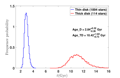
We obtain the kinematic age and uncertainty for stars in thin disk (1,894 stars) and thick disk (114 stars) with the methods described at the beginning of section 4.3. The typical ages are $2.84^{+0.32}_{-0.26}$ Gyr, $10.42^{+1.82}_{-0.73}$ for thin and thick disk respectively. As shown in Figure 17, the age distribution of stars in the thick disk is generally larger than 8 Gyr, while the thin disk is populated by younger stars. This is well consistent with previous studies (Fuhrmann, 1998; Bensby et al., 2003; Haywood et al., 2013; Bensby et al., 2014).

To explore the relation between $TD/D$ and kinematic age, we first sorted the plant host sample by the relative probabilities for the thick-disk-to-thin-disk, i.e., $TD/D$. Next, according to $TD/D$, we divided the planet host sample into 10 bins with approximately equal size. Then, for each bin, we calculated their kinematic ages. As shown in Figure 18, the kinematic age generally increase with $TD/D$, demonstrating that $TD/D$ is a indicator of age for stars in the Galactic disk.

Figure 19: The comparison of radial velocities (RV) from different sources: (a). $\rm LAMOST\_RV$ vs. $\rm APOGEE\_RV$; (b). $\rm Gaia\_RV$ vs. $\rm APOGEE\_RV$; (c) $\rm EA\_RV$ vs. $\rm APOGEE\_RV$. The black lines in the figure indicate where the horizontal and vertical coordinates are equal. $\Delta RV$ represents the systematic offset in RV comparing to APOGEE measurements.

Figure 20: Distributions of the asteroseismic age (blue), kinematic age (red) and isochrone age (green) of 54 Kepler stars.

5 Discussions

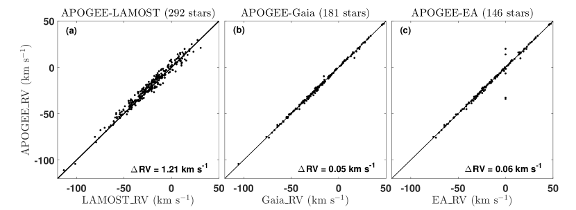
5.1 Systematic Differences in Radial Velocity from Various Sources

As mentioned in section 4.1.3, we obtained the RV from five sources: APOGEE, LAMOST, RAVE, Gaia, and EA. As the RV is one of the basic parameters to calculate the Galactic velocity, the systematic differences in RV will induce differences in the Galactic velocity and then effect the classification of Galactic components. Therefore, it is necessary to calibrate the systematic difference in RV from various sources.

Here we choose the APOGEE RV data as standard reference because it has the highest resolution ($R\sim 22500$) and thus the most accurate RV measurements. Then we compare the difference in RV for common stars with measurements from the other sources overlapped with APOGEE : 292 for LAMOST, 2 for RAVE, 181 for Gaia, and 146 for EA. As shown in Figure 19, the systematic offsets in RV from APOGEE measurements, $\Delta RV$ are 1.21, 0.05, 0.06 $\rm km\ s^{-1}$ for LAMOST, Gaia, and EA respectively. For RAVE, there is only 2 common stars and too few to make analysis. Here we refer to Huang et al. (2018), which presents a new catalog of RV standard stars selected from the APOGEE data and find that the systematic offset is only 0.17 $\rm km\ s^{-1}$ for RAVE. The systematic differences in RV between APOGEE and other sources are all smaller than the typical uncertainties in RV of our sample 1.58 $\rm km\ s^{-1}$ and thus have no significant influence in the calculation of Galactic velocity and the classification of Galactic components.

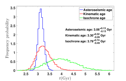
5.2 Kinematic Age vs. Asteroseismic Age vs. Isochrone Age

In order to access the reliability of kinematic ages derived in this work, we compare them to ages derived from asteroseismology and isochrone. The Kepler asteroseismic LEGACY sample (Silva Aguirre et al., 2017) provides a well characterized sample of 66 Kepler planet hosts with asteroseismic age estimates whose average uncertainy is $\sim 10\%$. Besides, Berger et al. (2020b) presents age estimates from isochrone fitting for 186,301 Gaia-Kepler stars with a median uncertainties of 56%. By cross-matching our planet host catalog (Table 10) with the samples in the above two studies, we obtained a common sample of 54 Kepler planet hosts. In Figure 20, we compare the distributions of median asteroseismic age, median ischrone age and kinematic age for the common sample. The distributions of median asteroseismic age and median ischrone age were constructed by 10,000 sets of resampled ages based on the reported ages and uncertainties (assuming Gaussian distribution $N(t,\sigma_{t})$). The distribution of kinematic ages were constructed with AVR from Equation 15 using a Monte Carlo method which took into account the uncertainties of AVR parameters (Table 4) and velocity dispersions. As can be seen in Figure 20, the results are $3.06^{+0.13}_{-0.13}$ Gyr, $3.30^{+0.32}_{-0.28}$ Gyr and $3.79^{+0.74}_{-0.49}$ Gyr for asteroseismic age, kinematic age, and isochrone age, respectively. Encouragingly, our kinematic ages match better with the asteroseismic ages, though the three kinds of ages are not inconsistent with each other within their errorbars.

5.3 Future Studies

For the clarity and simplicity of the paper, here we apply the revised kinematic methods (section 2 and 3) only to the planet host sample. Next, in our second paper of the PAST project (Chen et al. in prep.), we will apply the revised kinematic methods to the whole Kepler star sample, enabling us to further connect stellar kinematic properties to stellar rotations and activities.

The planet host catalog provides stellar parameters, spatial position, Galactic velocity and component classification for 2,174 stars, which hosts 2,872 planets. Furthermore, using AVR as we show in section 3.6, one can obtain the kinematic age for a group of stars with respective properties. As shown in Figure 13 and Table 7, these planet hosts spread over different Galactic components in a wide range of distance up to $~{}1,500$ pc. With such rich stellar information, future studies are allowed to explore and answer some fundamental questions on exoplanets, such as, what are the differences in various properties of planetary systems at different positions in the Galaxy with different ages? Specifically, in a subsequent paper of the PAST project (Yang et al. in prep), we will study whether/how planetary occurrence and architecture change with the Galactic environment. The answers of these questions will be crucial in constraining various models and theories of planetary formation and evolution.

6 Guidelines for Using the Methods and Catalog

In this section, we provide the guidelines, cautions and limitations to utilize the revised kinematic methods (section 2 and 3) and planet host catalog (Table 10).

To classify stars into different Galactic components, the key is to calculate the relative probabilities between two different components (i.e. $TD/D,\ TD/H,\ Herc/D,\ Herc/D$) with Equation (4) and (5), which rely on the X factor and velocity ellipsoid (i.e. $\sigma_{U}$, $\sigma_{V}$, $\sigma_{W}$, and $V_{\rm asym}$) of different Galactic components. Here, we suggest two ways to obtain these kinematic parameters for a given Galactic position $(R,\ Z)$. The most easy way is to use our fitting formulae (e.g., Equation 7 with coefficients in Table 2 for $\sigma_{U}$, $\sigma_{V}$ and $\sigma_{W}$, and Equation 8 for $V_{\rm asym}$). Alternatively, one can conduct interpolation based on our revised characteristics in Table 9.

To derive the kinematic age for a group of stars, one can use the AVR (Equation 15) with the revised coefficients in Table 4. The typical age uncertainty can be estimated from Equation 16, which is $\sim 10-20\%$ here. For the purpose of avoiding potential spacial biases, we recommend to adopt the total velocity dispersion (Equation 13) when using the AVR (Equation 15).

Applying the above revised methods to our planet host sample, we provide a catalog with kinematic properties (e.g. Galactic position, velocity and $TD/D$) and other basic parameters (e.g. $T_{\rm eff}$ and element abundances). With this catalog, one can divide planet hosts into bins according to respective properties (e.g., planetary period, multiplicity etc.) and calculate the kinematic age for each bin, which will be practical and useful for statistical studies of age effects on planetary systems. Although the kinematic method can not directly measure the ages for individual stars, some of the derived kinematic properties (e.g., $TD/D$) could serve as good age tracers given their significant correlations (e.g., Figure 18).

However, there are some notable cautions and limitations, which are listed as follows:

(1). The revised velocity ellipsoid and AVR are strictly applicable for stars within the region calibration sample covers, i.e, within 1.54 kpc to the Sun (corresponding to $R=7.5-10.0$ kpc, $|\theta|<10$ deg $\&\ |Z|=0-1.5$ kpc). Taking the assumption that the Galactic disk is axis-symmetric (e.g. Yurin & Springel, 2014; Aumer et al., 2016), the velocity ellipsoid and AVR will be indenpent of $\theta$ (e.g. Williams et al., 2013). Thus the criterion $|\theta|<10$ deg are not necessary for the Galactic disk stars. Besides, with Equation 7 and Table 2, the velocity dispersion can be extrapolated to the region outer to 1.54 kpc. However, this extrapolation should be adopted with caution.

(2). Since the additional motions caused by binary orbits could affect the stellar kinematic, binaries should be applied with caution.

(3). Due to the small numbers of Halo and Hercules stream stars in our calibration sample, we adopt the velocity dispersion values derived from stars in the solar neighborhood as in Bensby et al. (2014). As the velocity dispersions change with the Galactic position (Williams et al., 2013), there might be some deviations in the classification of Halo and Hercules stream stars when utilizing the characteristic parameters in Table 9 and the planet host catalog in Table 10. It will be more reliable to take other parameters (e.g. velocity, element abundance, angular momentum Bensby et al., 2007; Lee et al., 2011; Bonaca et al., 2017; Kushniruk & Bensby, 2019) into consideration.

(4). There is no clear trend between velocity dispersions and ages for stars belong to Hercules stream and halo in our calibration sample. Therefore, the method to derive kinematic age is only suitable for stars in the Galactic disk.

(5). The kinematic ages and uncertainties derived from Equation 15 and 16 are the typical (median/mean) values for a group of stars.

7 Summary

Since 1995, the discovered exoplanet population has expanded significantly from the solar neighborhood to a much larger area in the Galaxy (Figure 1). We are therefore entering a new era to study exoplanets in a big context of the Galaxy. In the Galactic context, the relations between the properties of planetary systems and the kinematics as well as the ages of planet host stars have yet to be explored. To answer these questions, we perform a series of studies in a project dubbed as PAST (Planets Across Space and Time). In this paper, as the Paper I and the basis of the PAST series, we revisit the kinematic methods for classification of Galactic components (section 2) and estimation of kinematic ages (section 3) and apply them to planet host stars (section 4).

For classification of Galactic components (section 2), we adopt the well-used kinematic approach as in Bensby et al. (2003, 2014). However, so far, the kinematic characteristics of this method has been applied only to the Solar neighborhood within $\sim 100-200$ pc. For this reason, using a calibration sample based on the GAIA and LAMOST data (section 2.3.1), we extend the kinematic characteristics to $\sim 1,500$ pc (section 2.3, Table 9) to cover the majority of planet hosts (Figure 1 and 13).

For estimation of kinematic ages, we refit the Age-Velocity dispersion Relation (AVR) with the calibration sample (section 3, Figure 8). Our AVR is consistent with those in previous studies (e.g., Holmberg et al. (2009)) but with much smaller internal uncertainties (Table 4) thanks to the large and high quality calibration sample. Based on this refined AVR, we are able to derive kinematic age with an uncertainty of 10-20% (section 3.6), which is a factor of $\sim$3 smaller than those from previous studies (Table 5).

Applying the above revised methods to our planet host sample, we then construct a catalog with kinematic properties and other basic parameters for 2,174 stars (section 4.2, Table 10) by combining data from Gaia, LAMOST, APOGEE, RAVE and the NASA exoplanet archive (Table 6 and section 4.1). The majority (1,894/2,174, 87.1%) of planet host stars are found to be in the Galactic thin disk, while 5.2% (114/2,174) of them belong to the thick disk and only 0.05% (1/2,174) reside in the halo (Table 7). As expected, we find that the total velocity, $\rm[\alpha/Fe]$ and the kinematic age generally increase with the relative probabilities for the thick-disk-to-thin-disk, i.e., $TD/D$, while $\rm[Fe/H]$ decreases with $TD/D$ (Figure 15, 18). The kinematic age is $2.84^{+0.32}_{-0.26}$ Gyr for the thin disk stars and $10.42^{+1.82}_{-0.73}$ Gyr for the thick disk stars in the planet host sample (Figure 17).

We also compare our derived kinematic ages with asteroseismic ages and isochrone ages (section 5.2). Our kinematic ages match better with the asteroseismic ages, though the three kinds of ages are generally consistent with each other within their uncertainties (Figure 20).

Future studies of exoplanets in the Galactic context, e.g., the subsequent papers of our PAST series (section 5.3), will benefit not only from the catalog of the kinematic properties but also from the revised methods that derived such catalog in this work. The important guidelines, cautions and limitation when utilizing our kinematic methods and planet host catalog are described in section 6.

Table 9: Revised characteristics at different Galactic radii ($R$) and heights ($Z$) for different Galactic components using the calibration sample.

$|Z|$	$R$	$\sigma^{\rm D}_{\rm U}$	$\sigma^{\rm D}_{\rm V}$	$\sigma^{\rm D}_{\rm W}$	$V^{\rm D}_{\rm asym}$	$\sigma^{\rm TD}_{\rm U}$	$\sigma^{\rm TD}_{\rm V}$	$\sigma^{\rm TD}_{\rm W}$	$V^{\rm TD}_{\rm asym}$	$X_{\rm D}$	$X_{\rm TD}$	$X_{\rm H}$	$X_{\rm Herc}$
(kpc)	(kpc)	—————————  ($\rm km\ s^{-1}$)  —————————
$0-0.1$	$7.5-8.0$	37	22	15	$-16$	63	37	31	-41	0.81	0.13	0.0010	0.06
	$8.0-8.5$	34	21	16	$-14$	65	39	35	$-44$	0.84	0.10	0.0013	0.06
	$8.5-9.0$	35	20	16	$-15$	70	37	33	$-51$	0.85	0.10	0.0013	0.05
	$9.0-9.5$	33	19	15	$-12$	70	35	34	$-51$	0.87	0.09	0.0014	0.04
	$9.5-10.0$	33	19	16	$-11$	68	37	31	$-48$	0.89	0.08	0.0016	0.03
$0.1-0.2$	$7.5-8.0$	32	23	15	$-13$	69	37	39	$-43$	0.78	0.16	0.0011	0.06
	$8.0-8.5$	35	22	17	$-15$	66	42	36	-45	0.79	0.14	0.0010	0.07
	$8.5-9.0$	35	21	16	$-15$	71	41	36	-52	0.81	0.13	0.0014	0.06
	$9.0-9.5$	32	20	16	$-13$	71	42	34	$-52$	0.85	0.12	0.0012	0.04
	$9.5-10.0$	30	20	16	$-11$	70	40	34	$-50$	0.87	0.10	0.0019	0.03
$0.2-0.3$	$7.5-8.0$	36	22	16	$-16$	67	39	37	$-46$	0.75	0.20	0.0016	0.07
	$8.0-8.5$	37	23	17	$-17$	68	42	40	$-47$	0.76	0.17	0.0015	0.07
	$8.5-9.0$	37	22	18	$-17$	72	42	37	$-54$	0.78	0.16	0.0017	0.06
	$9.0-9.5$	34	21	16	$-14$	71	40	36	$-52$	0.81	0.14	0.0016	0.05
	$9.5-10.0$	31	21	16	$-11$	67	39	35	$-48$	0.84	0.13	0.0140	0.03
$0.3-0.4$	$7.5-8.0$	38	24	19	$-18$	68	41	38	-47	0.71	0.24	0.0016	0.05
	$8.0-8.5$	40	23	18	$-19$	68	41	41	$-47$	0.71	0.21	0.0020	0.08
	$8.5-9.0$	38	22	18	$-17$	71	41	38	$-52$	0.75	0.19	0.0020	0.06
	$9.0-9.5$	36	21	17	$-15$	71	42	37	$-52$	0.77	0.17	0.0020	0.06
	$9.5-10.0$	34	21	16	$-14$	71	41	35	$-52$	0.80	0.16	0.0025	0.04
$0.4-0.55$	$7.5-8.0$	42	26	18	$-21$	71	42	40	-52	0.65	0.29	0.0021	0.06
	$8.0-8.5$	41	24	19	$-21$	70	41	42	$-50$	0.66	0.26	0.0026	0.08
	$8.5-9.0$	39	23	18	$-19$	71	42	38	$-52$	0.70	0.23	0.0022	0.07
	$9.0-9.5$	37	22	16	$-17$	71	41	38	$-52$	0.73	0.21	0.0024	0.06
	$9.5-10.0$	37	22	16	$-16$	70	40	35	$-50$	0.75	0.19	0.0025	0.06
$0.55-0.75$	$7.5-8.0$	42	27	21	$-21$	71	45	41	-52	0.55	0.37	0.0042	0.08
	$8.0-8.5$	44	24	20	$-23$	72	43	42	$-54$	0.58	0.34	0.0035	0.08
	$8.5-9.0$	40	24	19	$-20$	72	43	40	$-54$	0.61	0.31	0.0026	0.08
	$9.0-9.5$	38	23	19	$-18$	72	43	40	$-52$	0.65	0.29	0.0026	0.06
	$9.5-10.0$	38	23	18	$-16$	71	40	40	$-52$	0.68	0.26	0.0029	0.06
$0.75-1.0$	$7.5-8.0$	45	29	23	$-24$	71	43	44	-52	0.43	0.48	0.0055	0.08
	$8.0-8.5$	45	26	21	$-22$	73	43	43	$-55$	0.46	0.45	0.0053	0.08
	$8.5-9.0$	42	23	20	$-21$	73	45	41	$-55$	0.50	0.42	0.0039	0.09
	$9.0-9.5$	39	23	20	$-19$	72	43	40	$-54$	0.56	0.36	0.0026	0.08
$1.0-1.5$	$7.5-8.0$	46	31	25	$-25$	72	45	46	-54	0.25	0.63	0.0129	0.10
	$8.0-8.5$	45	28	23	$-22$	73	45	44	$-55$	0.28	0.61	0.0100	0.10
	$8.5-9.0$	42	36	22	$-24$	73	45	43	$-55$	0.31	0.59	0.0103	0.09
	$9.0-9.5$	43	25	21	$-23$	74	45	40	$-57$	0.34	0.56	0.0056	0.09

Table 10: The catalogue of kinematic properties and other basic properties for the combined planet host stars

Column	Name	Format	Units	description
Parameters obtained from Gaia, APOGEE, RAVE, LAMOST and NASA exoplanet archive (EA)
1	Gaia_ID	Long		Unique Gaia source identifier
2	LAMOST_ID	string		LAMOST unique spectral ID
3	APOGEE_ID	string		APOGEE unique spectral ID
4	RAVE_ID	string		RAVE unique spectral ID
5	pl_hostname	string		NASA Exoplanet archive unique planet host name
6	Kepler_ID	integer		Kepler Input Catalog (KIC) ID
7	Gaia RA	Double	deg	Barycentric right ascension
8	Gaia Dec	Double	deg	Barycentric Declination
9	Gaia parallax	Double	mas	Absolute stellar parallax
10	Gaia e_parallax	Double	mas	Standard error of parallax
11	Gaia pmra	Double	mas $\rm yr^{-1}$	Proper motion in right ascension direction
12	Gaia e_pmra	Double	mas $\rm yr^{-1}$	Standard error of proper motion in right ascension direction
13	Gaia pmdec	Double	mas $\rm yr^{-1}$	Proper motion in declination direction
14	Gaia e_pmdec	Double	mas $\rm yr^{-1}$	Standard error of proper motion in declination direction
15	Gaia G mag	Double	mag	Gaia G band apparent magnitude
16	$T_{\rm eff}$	Float	K	Effective temperature from RAVE, LAMOST, APOGEE, Gaia, EA
17	${\rm flag}\_T_{\rm eff}^{1}$	integer		flag represents which source each value is collected from
18	$\log g$	Float		Surface gravity from RAVE, LAMOST, APOGEE, Gaia, EA
19	${\rm flag}\_\log g^{1}$	integer		flag represents which source each value is collected from
20	$\rm[Fe/H]$	Float	dex	Metallicity from RAVE, LAMOST, APOGEE, Gaia, EA
21	${\rm flag}\_{\rm[Fe/H]}^{1}$	integer		flag represents which source each value is collected from
22	$\rm[\alpha/Fe]$	Float	dex	$\rm\alpha$ elements abundance from RAVE, LAMOST, APOGEE, Gaia, EA
23	${\rm flag}\_{\rm[\alpha/Fe]}^{1}$	integer		flag represents which source each value is collected from
24	rv	Double	km $\rm s^{-1}$	Radial velocity from APOGEE, RAVE, Gaia, LAMOST, EA
25	e_rv	Double	km $\rm s^{-1}$	Error of radial velocity
26	${\rm flag}\_{\rm rv}^{1}$	integer		flag represents which source each value is collected from
Parameters derived in this work
27	$R$	Double	kpc	Galactocentric Cylindrical radial distance
28	$\theta$	Double	deg	Galactocentric Cylindrical azimuth angle
29	$Z$	Double	kpc	Galactocentric Cylindrical vertical height
30	$V_{R}$	Double	km $\rm s^{-1}$	Galactocentric Cylindrical $R$ velocities
31	$V_{\theta}$	Double	km $\rm s^{-1}$	Galactocentric Cylindrical $\theta$ velocities
32	$V_{Z}$	Double	km $\rm s^{-1}$	Galactocentric Cylindrical $Z$ velocities
33	$U_{\rm LSR}$	Double	km $\rm s^{-1}$	Cartesian Galactocentric $X$ velocity to the LSR
34	e_$U_{\rm LSR}$	Double	km $\rm s^{-1}$	error of Cartesian Galactocentric $X$ velocity to the LSR
35	$V_{\rm LSR}$	Double	km $\rm s^{-1}$	Cartesian Galactocentric $Y$ velocity to the LSR
36	e_$V_{\rm LSR}$	Double	km $\rm s^{-1}$	error of Cartesian Galactocentric $Y$ velocity to the LSR
37	$W_{\rm LSR}$	Double	km $\rm s^{-1}$	Cartesian Galactocentric $Z$ velocity to the LSR
38	e_$W_{\rm LSR}$	Double	km $\rm s^{-1}$	error of Cartesian Galactocentric $Z$ velocity to the LSR
39	$TD/D$	Double		Thick disc to thin disc membership probability ratio
40	$TD/H$	Double		hick disc to halo membership probability ratio
41	$Her/D$	Double		Hercules stream to thin disc membership probability ratio
42	$Herc/TD$	Double		Hercules stream to thick disk membership probability ratio

References

- Adibekyan et al. (2013) Adibekyan, V. Z., Figueira, P., Santos, N. C., et al. 2013, A&A, 554, A44, doi: 10.1051/0004-6361/201321520
- Ahumada et al. (2020) Ahumada, R., Allende Prieto, C., Almeida, A., et al. 2020, ApJS, 249, 3, doi: 10.3847/1538-4365/ab929e
- Akeson et al. (2013) Akeson, R. L., Chen, X., Ciardi, D., et al. 2013, PASP, 125, 989, doi: 10.1086/672273
- Anglada-Escude et al. (2014) Anglada-Escude, G., Arriagada, P., Tuomi, M., et al. 2014, MNRAS, 443, L89, doi: 10.1093/mnrasl/slu076
- Aumer et al. (2016) Aumer, M., Binney, J., & Schönrich, R. 2016, MNRAS, 462, 1697, doi: 10.1093/mnras/stw1639
- Aumer & Binney (2009) Aumer, M., & Binney, J. J. 2009, MNRAS, 397, 1286, doi: 10.1111/j.1365-2966.2009.15053.x
- Aumer & Schönrich (2015) Aumer, M., & Schönrich, R. 2015, MNRAS, 454, 3166, doi: 10.1093/mnras/stv2252
- Balbi & Tombesi (2017) Balbi, A., & Tombesi, F. 2017, Scientific Reports, 7, 16626, doi: 10.1038/s41598-017-16110-0
- Bashi & Zucker (2019) Bashi, D., & Zucker, S. 2019, AJ, 158, 61, doi: 10.3847/1538-3881/ab27c9
- Bensby et al. (2003) Bensby, T., Feltzing, S., & Lundström, I. 2003, A&A, 410, 527, doi: 10.1051/0004-6361:20031213
- Bensby et al. (2014) Bensby, T., Feltzing, S., & Oey, M. S. 2014, A&A, 562, A71, doi: 10.1051/0004-6361/201322631
- Bensby et al. (2007) Bensby, T., Oey, M. S., Feltzing, S., & Gustafsson, B. 2007, ApJ, 655, L89, doi: 10.1086/512014
- Berger et al. (2020a) Berger, T. A., Huber, D., Gaidos, E., van Saders, J. L., & Weiss, L. M. 2020a, AJ, 160, 108, doi: 10.3847/1538-3881/aba18a
- Berger et al. (2020b) Berger, T. A., Huber, D., van Saders, J. L., et al. 2020b, AJ, 159, 280, doi: 10.3847/1538-3881/159/6/280
- Binney et al. (2000) Binney, J., Dehnen, W., & Bertelli, G. 2000, MNRAS, 318, 658, doi: 10.1046/j.1365-8711.2000.03720.x
- Binney & Tremaine (2008) Binney, J., & Tremaine, S. 2008, Galactic Dynamics: Second Edition
- Binney et al. (2014) Binney, J., Burnett, B., Kordopatis, G., et al. 2014, MNRAS, 439, 1231, doi: 10.1093/mnras/stt2367
- Binney et al. (1997) Binney, J. J., Dehnen, W., Houk, N., Murray, C. A., & Penston, M. J. 1997, in ESA Special Publication, Vol. 402, Hipparcos - Venice ’97, ed. R. M. Bonnet, E. Høg, P. L. Bernacca, L. Emiliani, A. Blaauw, C. Turon, J. Kovalevsky, L. Lindegren, H. Hassan, M. Bouffard, B. Strim, D. Heger, M. A. C. Perryman, & L. Woltjer, 473–478
- Bonaca et al. (2017) Bonaca, A., Conroy, C., Wetzel, A., Hopkins, P. F., & Kereš, D. 2017, ApJ, 845, 101, doi: 10.3847/1538-4357/aa7d0c
- Bovy et al. (2012a) Bovy, J., Rix, H.-W., Liu, C., et al. 2012a, ApJ, 753, 148, doi: 10.1088/0004-637X/753/2/148
- Bovy et al. (2016) Bovy, J., Rix, H.-W., Schlafly, E. F., et al. 2016, ApJ, 823, 30, doi: 10.3847/0004-637X/823/1/30
- Bovy et al. (2012b) Bovy, J., Allende Prieto, C., Beers, T. C., et al. 2012b, ApJ, 759, 131, doi: 10.1088/0004-637X/759/2/131
- Büdenbender et al. (2015) Büdenbender, A., van de Ven, G., & Watkins, L. L. 2015, MNRAS, 452, 956, doi: 10.1093/mnras/stv1314
- Buder et al. (2018) Buder, S., Asplund, M., Duong, L., et al. 2018, MNRAS, 478, 4513, doi: 10.1093/mnras/sty1281
- Chaplin et al. (2014) Chaplin, W. J., Basu, S., Huber, D., et al. 2014, ApJS, 210, 1, doi: 10.1088/0067-0049/210/1/1
- Chen et al. (2001) Chen, B., Stoughton, C., Smith, J. A., et al. 2001, ApJ, 553, 184, doi: 10.1086/320647
- Cheng et al. (2012) Cheng, J. Y., Rockosi, C. M., Morrison, H. L., et al. 2012, ApJ, 752, 51, doi: 10.1088/0004-637X/752/1/51
- Cui et al. (2012) Cui, X.-Q., Zhao, Y.-H., Chu, Y.-Q., et al. 2012, Research in Astronomy and Astrophysics, 12, 1197, doi: 10.1088/1674-4527/12/9/003
- De Cat et al. (2015) De Cat, P., Fu, J. N., Ren, A. B., et al. 2015, ApJS, 220, 19, doi: 10.1088/0067-0049/220/1/19
- Dehnen & Binney (1998) Dehnen, W., & Binney, J. J. 1998, MNRAS, 298, 387, doi: 10.1046/j.1365-8711.1998.01600.x
- Deng et al. (2012) Deng, L.-C., Newberg, H. J., Liu, C., et al. 2012, Research in Astronomy and Astrophysics, 12, 735, doi: 10.1088/1674-4527/12/7/003
- Everall et al. (2019) Everall, A., Evans, N. W., Belokurov, V., & Schönrich, R. 2019, MNRAS, 489, 910, doi: 10.1093/mnras/stz2217
- Famaey et al. (2005) Famaey, B., Jorissen, A., Luri, X., et al. 2005, A&A, 430, 165, doi: 10.1051/0004-6361:20041272
- Feltzing et al. (2003) Feltzing, S., Bensby, T., & Lundström, I. 2003, A&A, 397, L1, doi: 10.1051/0004-6361:20021661
- Fuhrmann (1998) Fuhrmann, K. 1998, A&A, 338, 161
- Gai et al. (2011) Gai, N., Basu, S., Chaplin, W. J., & Elsworth, Y. 2011, ApJ, 730, 63, doi: 10.1088/0004-637X/730/2/63
- Gaia Collaboration et al. (2016) Gaia Collaboration, Prusti, T., de Bruijne, J. H. J., et al. 2016, A&A, 595, A1, doi: 10.1051/0004-6361/201629272
- Gaia Collaboration et al. (2018a) Gaia Collaboration, Brown, A. G. A., Vallenari, A., et al. 2018a, A&A, 616, A1, doi: 10.1051/0004-6361/201833051
- Gaia Collaboration et al. (2018b) Gaia Collaboration, Katz, D., Antoja, T., et al. 2018b, A&A, 616, A11, doi: 10.1051/0004-6361/201832865
- Gilmore et al. (1989) Gilmore, G., Wyse, R. F. G., & Kuijken, K. 1989, ARA&A, 27, 555, doi: 10.1146/annurev.aa.27.090189.003011
- Gomez et al. (1997) Gomez, A. E., Grenier, S., Udry, S., et al. 1997, in ESA Special Publication, Vol. 402, Hipparcos - Venice ’97, ed. R. M. Bonnet, E. Høg, P. L. Bernacca, L. Emiliani, A. Blaauw, C. Turon, J. Kovalevsky, L. Lindegren, H. Hassan, M. Bouffard, B. Strim, D. Heger, M. A. C. Perryman, & L. Woltjer, 621–624
- Gonzalez et al. (2001) Gonzalez, G., Brownlee, D., & Ward, P. 2001, Icarus, 152, 185, doi: 10.1006/icar.2001.6617
- Gowanlock et al. (2011) Gowanlock, M. G., Patton, D. R., & McConnell, S. M. 2011, Astrobiology, 11, 855, doi: 10.1089/ast.2010.0555
- Guinan et al. (2016) Guinan, E. F., Engle, S. G., & Durbin, A. 2016, ApJ, 821, 81, doi: 10.3847/0004-637X/821/2/81
- Guo et al. (2016) Guo, J.-C., Liu, C., & Liu, J.-F. 2016, Research in Astronomy and Astrophysics, 16, 44, doi: 10.1088/1674-4527/16/3/044
- Guo et al. (2019) Guo, J.-C., Zhang, H.-W., Huang, Y., et al. 2019, Research in Astronomy and Astrophysics, 19, 008, doi: 10.1088/1674-4527/19/1/8
- Haywood et al. (2013) Haywood, M., Di Matteo, P., Lehnert, M. D., Katz, D., & Gómez, A. 2013, A&A, 560, A109, doi: 10.1051/0004-6361/201321397
- Ho et al. (2017) Ho, A. Y. Q., Rix, H.-W., Ness, M. K., et al. 2017, ApJ, 841, 40, doi: 10.3847/1538-4357/aa6db3
- Holmberg et al. (2009) Holmberg, J., Nordström, B., & Andersen, J. 2009, A&A, 501, 941, doi: 10.1051/0004-6361/200811191
- Holtzman et al. (2018) Holtzman, J. A., Hasselquist, S., Shetrone, M., et al. 2018, AJ, 156, 125, doi: 10.3847/1538-3881/aad4f9
- Hou et al. (2013) Hou, J. L., Zhong, J., Chen, L., et al. 2013, in IAU Symposium, Vol. 292, Molecular Gas, Dust, and Star Formation in Galaxies, ed. T. Wong & J. Ott, 105–105, doi: 10.1017/S1743921313000653
- Huang et al. (2018) Huang, Y., Liu, X. W., Chen, B. Q., et al. 2018, AJ, 156, 90, doi: 10.3847/1538-3881/aacda5
- Jiménez-Torres et al. (2013) Jiménez-Torres, J. J., Pichardo, B., Lake, G., & Segura, A. 2013, Astrobiology, 13, 491, doi: 10.1089/ast.2012.0842
- Jofré & Weiss (2011) Jofré, P., & Weiss, A. 2011, A&A, 533, A59, doi: 10.1051/0004-6361/201117131
- Johnson & Soderblom (1987) Johnson, D. R. H., & Soderblom, D. R. 1987, AJ, 93, 864, doi: 10.1086/114370
- Jordi et al. (2010) Jordi, C., Gebran, M., Carrasco, J. M., et al. 2010, A&A, 523, A48, doi: 10.1051/0004-6361/201015441
- Kalirai (2012) Kalirai, J. S. 2012, Nature, 486, 90, doi: 10.1038/nature11062
- Kunder et al. (2017) Kunder, A., Kordopatis, G., Steinmetz, M., et al. 2017, AJ, 153, 75, doi: 10.3847/1538-3881/153/2/75
- Kushniruk & Bensby (2019) Kushniruk, I., & Bensby, T. 2019, A&A, 631, A47, doi: 10.1051/0004-6361/201935234
- Lee et al. (2011) Lee, Y. S., Beers, T. C., An, D., et al. 2011, ApJ, 738, 187, doi: 10.1088/0004-637X/738/2/187
- Lineweaver et al. (2004) Lineweaver, C. H., Fenner, Y., & Gibson, B. K. 2004, Science, 303, 59, doi: 10.1126/science.1092322
- Liu et al. (2014) Liu, X. W., Yuan, H. B., Huo, Z. Y., et al. 2014, in IAU Symposium, Vol. 298, Setting the scene for Gaia and LAMOST, ed. S. Feltzing, G. Zhao, N. A. Walton, & P. Whitelock, 310–321, doi: 10.1017/S1743921313006510
- Luo et al. (2012) Luo, A. L., Zhang, H.-T., Zhao, Y.-H., et al. 2012, Research in Astronomy and Astrophysics, 12, 1243, doi: 10.1088/1674-4527/12/9/004
- Mackereth et al. (2019) Mackereth, J. T., Bovy, J., Leung, H. W., et al. 2019, MNRAS, 489, 176, doi: 10.1093/mnras/stz1521
- Martig et al. (2016) Martig, M., Fouesneau, M., Rix, H.-W., et al. 2016, MNRAS, 456, 3655, doi: 10.1093/mnras/stv2830
- McTier & Kipping (2019) McTier, M. A. S., & Kipping, D. M. 2019, MNRAS, 489, 2505, doi: 10.1093/mnras/stz2088
- Ness et al. (2016) Ness, M., Hogg, D. W., Rix, H. W., et al. 2016, ApJ, 823, 114, doi: 10.3847/0004-637X/823/2/114
- Parenago (1950) Parenago, P. P. 1950, AZh, 27, 41
- Reddy et al. (2003) Reddy, B. E., Tomkin, J., Lambert, D. L., & Allende Prieto, C. 2003, VizieR Online Data Catalog, J/MNRAS/340/304
- Reid et al. (2014) Reid, M. J., Menten, K. M., Brunthaler, A., et al. 2014, ApJ, 783, 130, doi: 10.1088/0004-637X/783/2/130
- Rizzuto et al. (2018) Rizzuto, A. C., Vanderburg, A., Mann, A. W., et al. 2018, AJ, 156, 195, doi: 10.3847/1538-3881/aadf37
- Robin et al. (2017) Robin, A. C., Bienaymé, O., Fernández-Trincado, J. G., & Reylé, C. 2017, A&A, 605, A1, doi: 10.1051/0004-6361/201630217
- Robin et al. (2003) Robin, A. C., Reylé, C., Derrière, S., & Picaud, S. 2003, A&A, 409, 523, doi: 10.1051/0004-6361:20031117
- Schönrich (2012) Schönrich, R. 2012, MNRAS, 427, 274, doi: 10.1111/j.1365-2966.2012.21631.x
- Sharma et al. (2014) Sharma, S., Bland-Hawthorn, J., Binney, J., et al. 2014, ApJ, 793, 51, doi: 10.1088/0004-637X/793/1/51
- Silva Aguirre et al. (2017) Silva Aguirre, V., Lund, M. N., Antia, H. M., et al. 2017, ApJ, 835, 173, doi: 10.3847/1538-4357/835/2/173
- Soderblom (2010) Soderblom, D. R. 2010, ARA&A, 48, 581, doi: 10.1146/annurev-astro-081309-130806
- Stojković et al. (2019) Stojković, N., Vukotić, B., Martinović, N., Ćirković, M. M., & Micic, M. 2019, MNRAS, 490, 408, doi: 10.1093/mnras/stz2519
- Strömberg (1946) Strömberg, G. 1946, ApJ, 104, 12, doi: 10.1086/144830
- Su & Cui (2004) Su, D.-Q., & Cui, X.-Q. 2004, Chinese J. Astron. Astrophys., 4, 1, doi: 10.1088/1009-9271/4/1/1
- Sundin (2006) Sundin, M. 2006, International Journal of Astrobiology, 5, 325, doi: 10.1017/S1473550406003065
- Thompson et al. (2018) Thompson, S. E., Coughlin, J. L., Hoffman, K., et al. 2018, ApJS, 235, 38, doi: 10.3847/1538-4365/aab4f9
- Tian et al. (2015) Tian, H.-J., Liu, C., Carlin, J. L., et al. 2015, ApJ, 809, 145, doi: 10.1088/0004-637X/809/2/145
- Torres et al. (2019) Torres, S., Cantero, C., Camisassa, M. E., et al. 2019, A&A, 629, L6, doi: 10.1051/0004-6361/201936244
- van Leeuwen (2007) van Leeuwen, F. 2007, A&A, 474, 653, doi: 10.1051/0004-6361:20078357
- Wang et al. (1996) Wang, S.-G., Su, D.-Q., Chu, Y.-Q., Cui, X., & Wang, Y.-N. 1996, Appl. Opt., 35, 5155, doi: 10.1364/AO.35.005155
- Wielen (1977) Wielen, R. 1977, A&A, 60, 263
- Williams et al. (2013) Williams, M. E. K., Steinmetz, M., Binney, J., et al. 2013, MNRAS, 436, 101, doi: 10.1093/mnras/stt1522
- Wu et al. (2011) Wu, Y., Luo, A. L., Li, H.-N., et al. 2011, Research in Astronomy and Astrophysics, 11, 924, doi: 10.1088/1674-4527/11/8/006
- Wu et al. (2018) Wu, Y., Xiang, M., Bi, S., et al. 2018, MNRAS, 475, 3633, doi: 10.1093/mnras/stx3296
- Wylie-de Boer et al. (2010) Wylie-de Boer, E., Freeman, K., & Williams, M. 2010, AJ, 139, 636, doi: 10.1088/0004-6256/139/2/636
- Xiang et al. (2017a) Xiang, M., Liu, X., Shi, J., et al. 2017a, ApJS, 232, 2, doi: 10.3847/1538-4365/aa80e4
- Xiang et al. (2015) Xiang, M. S., Liu, X. W., Yuan, H. B., et al. 2015, MNRAS, 448, 822, doi: 10.1093/mnras/stu2692
- Xiang et al. (2017b) —. 2017b, MNRAS, 467, 1890, doi: 10.1093/mnras/stx129
- Yu & Liu (2018) Yu, J., & Liu, C. 2018, MNRAS, 475, 1093, doi: 10.1093/mnras/stx3204
- Yurin & Springel (2014) Yurin, D., & Springel, V. 2014, MNRAS, 444, 62, doi: 10.1093/mnras/stu1421
- Zhao et al. (2012) Zhao, G., Zhao, Y.-H., Chu, Y.-Q., Jing, Y.-P., & Deng, L.-C. 2012, Research in Astronomy and Astrophysics, 12, 723, doi: 10.1088/1674-4527/12/7/002
- Zhu et al. (2017) Zhu, W., Udalski, A., Novati, S. C., et al. 2017, AJ, 154, 210, doi: 10.3847/1538-3881/aa8ef1