L2E: Learning to Exploit Your Opponent
Abstract
Opponent modeling is essential to exploit sub-optimal opponents in strategic interactions. Most previous works focus on building explicit models to directly predict the opponents’ styles or strategies, which require a large amount of data to train the model and lack adaptability to unknown opponents. In this work, we propose a novel Learning to Exploit (L2E) framework for implicit opponent modeling. L2E acquires the ability to exploit opponents by a few interactions with different opponents during training, thus can adapt to new opponents with unknown styles during testing quickly. We propose a novel opponent strategy generation algorithm that produces effective opponents for training automatically. We evaluate L2E on two poker games and one grid soccer game, which are the commonly used benchmarks for opponent modeling. Comprehensive experimental results indicate that L2E quickly adapts to diverse styles of unknown opponents.
1 Introduction
One core research topic in modern artificial intelligence is creating agents that can interact effectively with their opponents in different scenarios. To achieve this goal, the agents should have the ability to reason about their opponents’ behaviors, goals, and beliefs. Opponent modeling, which constructs the opponents’ models, has been extensively studied in past decades (Albrecht & Stone, 2018). In general, an opponent model is a function that takes some interaction history as input and predicts some property of interest of the opponent. Specifically, the interaction history may contain the past actions that the opponent took in various situations, and the properties of interest could be the actions that the opponent may take in the future, the style of the opponent (e.g., “defensive”, “aggressive”), or its current goals. The resulting opponent model can inform the agent’s decision-making by incorporating the model’s predictions in its planning procedure to optimize its interactions with the opponent. Opponent modeling has already been used in many practical applications, such as dialogue systems (Grosz & Sidner, 1986), intelligent tutor systems (McCalla et al., 2000), and security systems (Jarvis et al., 2005).
Many opponent modeling algorithms vary greatly in their underlying assumptions and methodology. For example, policy reconstruction based methods (Powers & Shoham, 2005; Banerjee & Sen, 2007) explicitly fit an opponent model to reflect the opponent’s observed behaviors. Type reasoning based methods (Dekel et al., 2004; Nachbar, 2005) reuse pre-learned models of several known opponents by finding the one that most resembles the current opponent’s behavior. Classification based methods (Huynh et al., 2006; Sukthankar & Sycara, 2007) build models that predict the opponent’s play style, and employ the counter-strategy, which is effective against that particular style. Some recent works combine opponent modeling with deep learning methods or reinforcement learning methods and propose many related algorithms (He et al., 2016; Foerster et al., 2018; Wen et al., 2018). Although these algorithms have achieved some success, they also have two obvious disadvantages: 1) constructing accurate opponent models requires a lot of data, which is problematic since the agent may not have the time or opportunity to collect enough data about its opponent in most applications; and 2) most of these algorithms perform well only when the opponents during testing are similar to the ones used for training, thus it is difficult for them to adapt to opponents with new styles quickly.
To overcome these shortcomings, we propose a novel Learning to Exploit (L2E) framework in this work for implicit opponent modeling, which has two desirable advantages. First, L2E does not build an explicit model for the opponent, so it does not require a large amount of interactive data and simultaneously eliminates the modeling errors. Second, L2E can quickly adapt to new opponents with unknown styles, with only a few interactions with them. The key idea underlying L2E is to train a base policy against various opponents’ styles by using only a few interactions between them during training, such that it acquires the ability to exploit different opponents quickly. After training, the base policy can quickly adapt to new opponents using only a few interactions during testing. In effect, our L2E framework optimizes for a base policy that is easy and fast to adapt. It can be seen as a particular case of learning to learn, i.e., meta-learning (Finn et al., 2017). The meta-learning algorithm, such as MAML (Finn et al., 2017), is initially designed for single-agent environments. It requires the manual design of training tasks, and the final performance largely depends on the user-specified training task distribution. The L2E framework is designed explicitly for multi-agent competitive environments, which automatically generates effective training tasks (opponents). Some recent works have also initially used meta-learning for opponent modeling. Unlike these works, which either use meta-learning to predict the opponent’s behaviors (Rabinowitz et al., 2018) or handle the non-stationary problem in multi-agent reinforcement learning (Al-Shedivat et al., 2018), we focus on improving the agent’s ability to adapt to unknown opponents quickly.
In our L2E framework, the base policy is explicitly trained such that a few interactions with a new opponent will produce an opponent-specific policy to exploit this opponent effectively, i.e., the base policy has strong adaptability that is broadly adaptive to many opponents. Specifically, if a deep neural network models the base policy, then the opponent-specific policy can be obtained by fine-tuning the parameters of the base policy’s network using the new interactive data with the opponent. A critical step in L2E is how to generate effective opponents to train the base policy. The ideal training opponents should satisfy the following two desiderata. 1) The opponents need to be challenging enough (i.e., hard to exploit). By learning to exploit these challenging opponents, the base policy eliminates the weakness in its adaptability and learns a more robust strategy. 2) The opponents need to have enough diversity. The more diverse the opponents during training, the stronger the base policy’s generalization ability is, and the more adaptable the base policy to the new opponents.
To this end, we propose a novel opponent strategy generation (OSG) algorithm, which can produce challenging and diverse opponents automatically. We use the idea of adversarial training to generate challenging opponents. Some previous works have also been proposed to obtain more robust policies through adversarial training and improve generalization (Pinto et al., 2017; Pattanaik et al., 2018). From the perspective of the base policy, giving an opponent, the base policy first adjusts itself to obtain an adapted policy, the base policy is then optimized to maximize the rewards that the adapted policy gets when facing the opponent. The challenging opponents are then adversarially generated by minimizing the base policy’s adaptability by automatically generating difficult to exploit opponents. These hard-to-exploit opponents are trained such that even if the base policy adapts to them, the adapted base policy cannot take advantage of them. Besides, our OSG algorithm can further produce diverse training opponents with a novel diversity-regularized policy optimization procedure. In specific, we use the Maximum Mean Discrepancy (MMD) metric (Gretton et al., 2007) to evaluate the differences between policies. The MMD metric is then incorporated as a regularization term into the policy optimization process to obtain a diverse set of opponent policies. By training with these challenging and diverse training opponents, the robustness and generalization ability of our L2E framework are significantly improved. To summarize, this work’s main contributions are listed below in three-fold:
-
•
We propose a novel learning to exploit (L2E) framework to exploit sub-optimal opponents without building explicit models for it. L2E can quickly adapt to unknown opponents using only a few interactions.
-
•
We propose to use an adversarial training procedure to generate challenging opponents automatically. These hard to exploit opponents help L2E eliminate the weakness in its adaptability effectively.
-
•
We further propose a diversity-regularized policy optimization procedure to generate diverse opponents automatically. L2E’s generalization ability is improved significantly by training with these diverse opponents.
We conduct extensive experiments to evaluate the L2E framework in three different environments. Comprehensive experimental results demonstrate that the base policy trained with L2E quickly exploits a wide range of opponents compared to other algorithms.
2 Related Work
2.1 Opponent Modeling
Opponent modeling is a long-standing research topic in artificial intelligence, and some of the earliest works go back to the early days of game theory research (Brown, 1951). The main goal of opponent modeling is to interact more effectively with other agents by building models to reason about their intentions, predicting their next moves or other properties (Albrecht & Stone, 2018). The commonly used opponent modeling methods can be roughly divided into policy reconstruction, classification, type-based reasoning, and recursive reasoning. Policy reconstruction methods (Mealing & Shapiro, 2015) reconstruct the opponents’ decision-making process by building models that make explicit predictions about their actions. Classification methods (Weber & Mateas, 2009; Synnaeve & Bessiere, 2011) produce models that assign class labels (e.g., “aggressive” or “defensive”) to the opponent and employ a precomputed strategy that is effective against that particular class of opponent. Type-based reasoning methods (He et al., 2016; Albrecht & Stone, 2017) assume that the opponent has one of several known types and update the belief using the new observations obtained during the real-time interactions. Recursive reasoning methods (Muise et al., 2015; de Weerd et al., 2017) model the nested beliefs (e.g., “I believe that you believe that I believe…”) and simulate the opponents’ reasoning processes to predict their actions. Unlike these existing methods, which usually require a large amount of interactive data to generate useful opponent models, our L2E framework does not explicitly model the opponent and acquires the ability to exploit different opponents by training with limited interactions with different styles of opponents.
2.2 Meta-Learning
Meta-learning is a new trend of research in the machine learning community that tackles learning to learn (Hospedales et al., 2020). It leverages experiences in the training phase to learn how to learn, acquiring the ability to generalize to new environments or new tasks. Recent progress in meta-learning has achieved impressive results ranging from classification and regression in supervised learning (Finn et al., 2017; Nichol et al., 2018) to new task adaption in reinforcement learning (Wang et al., 2016; Xu et al., 2018). Some recent works have also initially explored the application of meta-learning in opponent modeling. For example, the theory of mind network (ToMnet) (Rabinowitz et al., 2018) uses meta-learning to improve the predictions about the opponents’ future behaviors. Another related work (Al-Shedivat et al., 2018) uses meta-learning to handle the non-stationarity problem in multi-agent interactions. Unlike these methods, we focus on improving the agents’ ability to quickly adapt to different unknown opponents.
2.3 Strategy Generation
The automatic generation of effective opponent strategies for training is a critical step in our approach. Furthermore, how to generate diverse strategies has been preliminarily studied in the reinforcement learning community. In specific, diverse strategies can be obtained in various ways, including adding some diversity regularization to the optimization objective (Abdullah et al., 2019), randomly searching in some diverse parameter space (Plappert et al., 2018; Fortunato et al., 2018), using information-based strategy proposal (Eysenbach et al., 2018; Gupta et al., 2018), and searching diverse strategies with evolutionary algorithms (Agapitos et al., 2008; Wang et al., 2019; Jaderberg et al., 2017, 2019). More recently, researchers from DeepMind propose a league training paradigm to obtain a Grandmaster level StarCraft II AI (i.e., AlphaStar) by training a diverse league of continually adapting strategies and counter-strategies (Vinyals et al., 2019). Different from AlphaStar, our opponent strategy generation algorithm exploits adversarial training and diversity-regularized policy optimization to produce challenging and diverse opponents, respectively.
3 Method
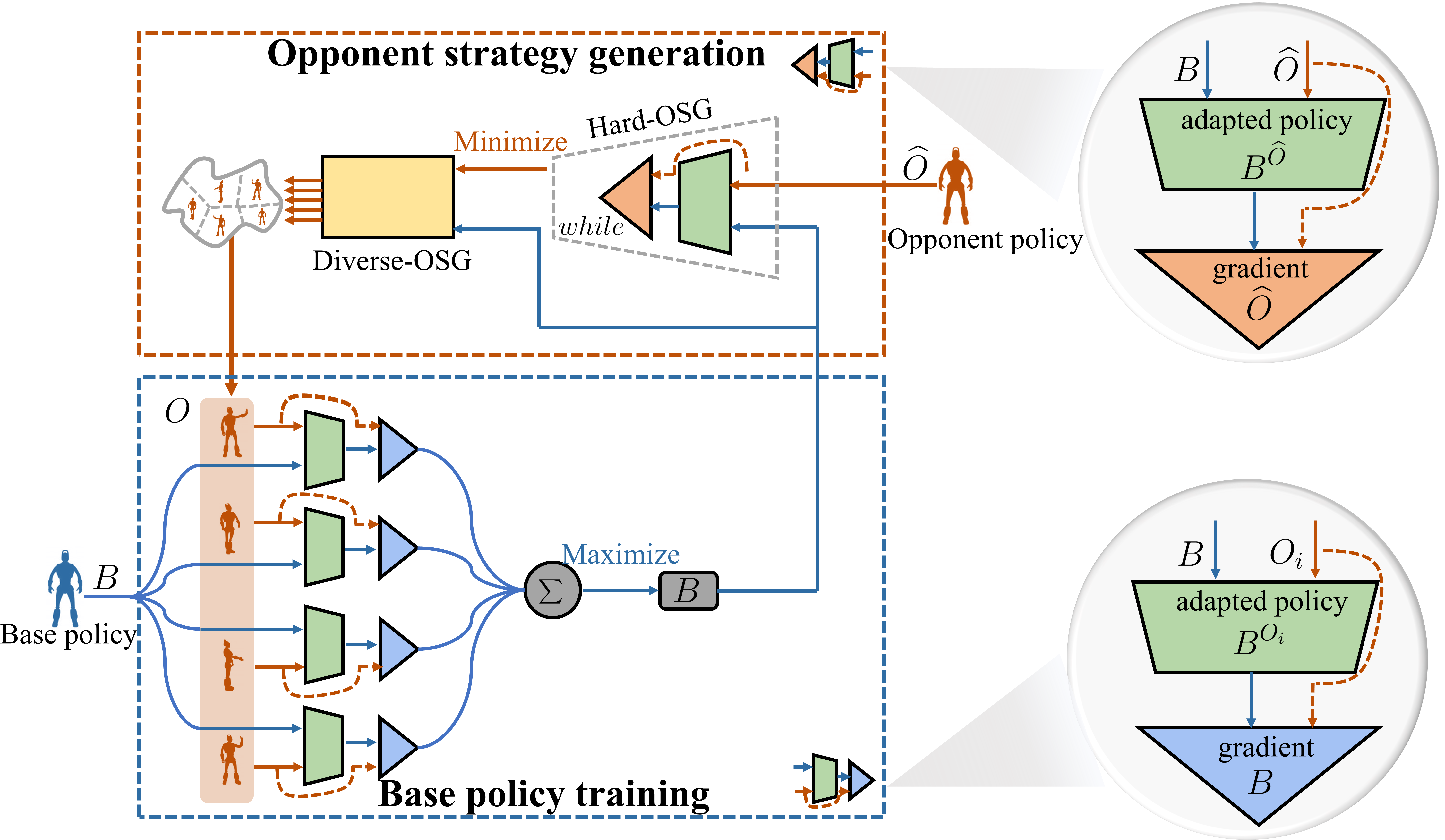
This paper proposes a novel L2E framework to endow the agents to adapt to diverse opponents quickly. As shown in Fig. 1, L2E mainly consists of two modules, i.e., the base policy training part and the opponent strategy generation part. In the base policy training part, our goal is to find a base policy that, given the unknown opponent, can fast adapt to it by using only a few interactions. To this end, the base policy is trained to be able to adapt to diverse opponents. In specific, giving an opponent , the base policy first adjusts itself to obtain an adapted policy by using a little interaction data between and , the base policy is then optimized to maximize the rewards that gets when facing . In other words, the base policy has learned how to adapt to its opponents and exploit them quickly.
The opponent strategy generation provides the base policy training part with challenging and diverse training opponents automatically. First, our proposed opponent strategy generation (OSG) algorithm can produce difficult-to-exploit opponents. In specific, the base policy first adjusts itself to obtain an adapted policy using a little interaction data between and , the opponent is then optimized to minimize the rewards that gets when facing . The resulting opponent is hard to exploit since even if the base policy adapts to , the adapted policy cannot take advantage of . By training with these hard to exploit opponents, the base policy can eliminate the weakness in its adaptability and improve its robustness effectively. Second, our OSG algorithm can further produce diverse training opponents with a novel diversity-regularized policy optimization procedure. More specifically, we first formalize the difference between opponent policies as the difference between the distribution of trajectories induced by each policy. The difference between distributions can be evaluated by the Maximum Mean Discrepancy (MMD) metric (Gretton et al., 2007). Then, MMD is integrated as a regularization term in the policy optimization process to identify various opponent policies. By training with these diverse opponents, the base policy’s generalization ability is improved significantly. Next, we introduce these two modules in detail.
3.1 Base Policy Training
Our goal is to find a base policy that can fast adapt to an unknown opponent by updating the parameters of using only a few interactions between and . The key idea is to train the base policy against many opponents to maximize its payoffs by using only a small amount of interactive data during training, such that it acquires the ability to exploit different opponents quickly. In effect, our L2E framework treats each opponent as a training example. After training, the resulting base policy can quickly adapt to new and unknown opponents using only a few interactions. Without loss of generality, the base policy is modeled by a deep neural network in this work, i.e., a parameterized function with parameters . Similarly, the opponent for training is also a deep neural network with parameters . We model the base policy as playing against an opponent in a two-player Markov game (Shapley, 1953). This Markov game consists of the state space , the action space and , and a state transition function where is a probability distribution on . The reward function for each player depends on the current state, the next state and both players’ actions. Given a training opponent whose policy is known and fixed, this two-player Markov game reduces to a single-player Markov Decision Process (MDP), i.e., . The state and action space of are the same as in . The transition and reward functions have the opponent policy embedded:
| (1) |
| (2) |
where the opponent’s action is sampled from its policy 111For brevity, we assume that environment is fully observable. More generally, agents use their observations to make decisions.. Throughout the paper, represents a single-player MDP, which is reduced from a two-player Markov game (i.e., player and player ). In this MDP, the player is fixed and can be regarded as part of the environment.
Suppose a set of training opponents is given. For each training opponent , an MDP can be constructed as described above. The base policy , i.e., is allowed to query a limited number of sample trajectories to adapt to . In our method, the adapted parameters of the base policy are computed using one or more gradient descent updates with the sample trajectories . For example, when using one gradient update:
| (3) |
| (4) |
represents that the trajectory is sampled from the MDP , where and .
We use to denote the updated base policy, i.e., . can be seen as an opponent-specific policy, which is updated from the base policy through fast adaptation. Our goal is to find a generalizable base policy whose opponent-specific policy can exploit its opponent as much as possible. To this end, we optimize the parameters of the base policy to maximize the rewards that gets when interacting with . More concretely, the learning to exploit objective function is defined as follows:
| (5) |
It is worth noting that the optimization is performed over the base policy’s parameters , whereas the objective is computed using the adapted based policy’s parameters . The parameters of the base policy are updated as follows:
| (6) |
In effect, our L2E framework aims to find a base policy that can significantly exploit the opponent with only a few interactions with it (i.e., with a few gradient steps). The resulting base policy has learned how to adapt to different opponents and exploit them quickly. An overall description of the base policy training procedure is shown in Alg. 1 which consists of three main steps. First, generating hard-to-exploit opponents through the Hard-OSG module (Section 3.2.1). Second, generating diverse opponent policies through the Diverse-OSG module (Section 3.2.2). Third, training the base policy with these opponents to obtain fast adaptability.
3.2 Automatic Opponent Generation
Previously, we assumed that the set of opponents had been given. How to automatically generate effective opponents for training is the key to the success of our L2E framework. The training opponents should be challenging enough (i.e., hard to exploit). By learning to exploit these hard-to-exploit opponents, the base policy can eliminate the weakness in its adaptability and become more robust. Besides, they should be sufficiently diverse. The more diverse they are, the stronger the generalization ability of the resulting base policy. We propose a novel opponent strategy generation (OSG) algorithm to achieve these goals.
3.2.1 Hard-to-Exploit Opponents Generation
We use the idea of adversarial learning to generate challenging training opponents for the base policy . From the perspective of the base policy , giving an opponent , first adjusts itself to obtain an adapted policy, i.e., the opponent-specific policy , the base policy is then optimized to maximize the rewards that gets when interacting with . Contrary to the base policy’s goal, we want to find a hard-to-exploit opponent for the current base policy , such that even if adapts to , the adapted policy cannot take advantage of . In other words, the hard-to-exploit opponent is trained to minimize the rewards that gets when interacting with . The base policy attempts to increase its adaptability by learning to exploit different opponents, while the hard-to-exploit opponent adversarially tries to minimize the base policy’s adaptability, i.e., maximize its counter-adaptability.
More concretely, the hard-to-exploit opponent is also a deep neural network with randomly initialized parameters . At each training iteration, an MDP can be constructed. The base policy first query a limited number of trajectories to adapt to . The parameters of the adapted policy are computed using one gradient descent update,
| (7) |
| (8) |
’s parameters are optimized to minimize the rewards that gets when interacting with . This is equivalent to maximizing the rewards that gets since we consider the two-player zero-sum competitive setting in this work. More concretely, the parameters are updated as follows:
| (9) |
| (10) |
After several rounds of iteration, we can obtain a hard-to-exploit opponent for the current base policy . The pseudo code of this hard-to-exploit training opponent generation algorithm is shown in Appendix B.1.
3.2.2 Diverse Opponents Generation
Training an effective base policy requires not only the hard-to-exploit opponents but also diverse opponents of different styles. The more diverse the opponents used for training, the stronger the generalization ability of the resulting base policy. From a human player’s perspective, the opponent style is usually defined as different types, such as aggressive, defensive, elusive, etc. The most significant difference between opponents with different styles lies in the actions taken in the same state. Take poker as an example, opponents of different styles tend to take different actions when holding the same hand. Based on the above analysis, we formalize the difference between opponent policies as the difference between the distribution of trajectories induced by each policy when interacting with the base policy. We argue that differences in trajectories better capture the differences between different opponent policies.
Formally, given a base policy , i.e., and an opponent policy , i.e., , our diversity-regularized policy optimization algorithm is to generate a new opponent , i.e., whose style is different from . We first construct two MDPs, i.e., and , and then sample two sets of trajectories, i.e., and from this two MDPs. The stochasticity in the MDP and the policy will induce a distribution over trajectories. We use the Maximum Mean Discrepancy (MMD) metric (Gretton et al., 2007) (see Appendix A for details) to measure the differences between and :
| (11) |
is the Gaussian radial basis function kernel defined over a pair of trajectories:
| (12) |
In our experiments, we found that simply setting the bandwidth to 1 produced satisfactory results. stacks the states and actions of a trajectory into a vector. For trajectories with different length, we clip the trajectories when both of them are longer than the minimum length . Usually, the trajectory’s length does not exceed , and we apply the masking based on the done signal from the environment to make them the same length.
There overall objective function of our proposed diversity-regularized policy optimization algorithm is as follows:
| (13) |
The first term is to maximize the rewards that gets when interacting with the base policy . The second one measures the difference between and the existing opponent . By this diversity-regularized policy optimization, the resulting opponent is not only good in performance but also diverse relative to the existing policy. Appendix A details the gradient calculation of the MMD term.
We can iteratively apply the above algorithm to find a set of distinct and diverse opponents. In specific, subsequent opponents are learned by encouraging diversity with respect to previously generated opponent set . The distance between an opponent and an opponent set is defined by the distance between and , where is the most similar policy to . Suppose we have obtained a set of opponents . The opponent, i.e., can be obtained by optimizing:
| (14) |
By doing so, the resulting opponent remains diverse relative to the opponent set . Appendix B.2 provides the pseudo code of the diverse training opponent generation algorithm.
4 Experiments

In this section, we conduct extensive experiments to evaluate the proposed L2E framework. We evaluate algorithm performance on the Leduc poker, the BigLeduc poker, and a Grid Soccer environment, the commonly used benchmark for opponent modeling (Lanctot et al., 2017; Steinberger, 2019; He et al., 2016). We first verify that the trained base policy using our L2E framework quickly exploit a wide range of opponents with only a few gradient updates. Then, we compare with other baseline methods to show the superiority of our L2E framework. Finally, we conduct a series of ablation experiments to demonstrate each part of our L2E framework’s effectiveness.
4.1 Rapid Adaptability
In this section, we verify the trained base policy’s ability to quickly adapt to different opponents in the Leduc poker environment (see Appendix C for more details). We provide four opponents with different styles and strengths. 1) The random opponent randomly takes actions whose strategy is relatively weak but hard to exploit since it does not have an evident decision-making style. 2) The call opponent always takes call actions and has a fixed decision-making style that is easy to exploit. 3) The rocks opponent takes actions based on its hand-strength, whose strategy is relatively strong. 4) The oracle opponent is a cheating and the strongest player who can see the other players’ hands and make decisions based on this perfect information.
As shown in Fig. 2, the base policy achieves a rapid increase in its average returns with a few gradient updates against all four opponent strategies. For the call opponent, which has a clear and monotonous style, the base policy can significantly exploit it. Against the random opponent with no clear style, the base policy can also exploit it quickly. When facing the strong rocks opponent or even the strongest oracle opponent, the base policy can quickly improve its average returns. One significant advantage of L2E is that the same base policy can exploit a wide range of opponents with different styles, demonstrating its strong generalization ability.
4.2 Comparisons with Other Baseline Methods
| Random | Call | Rocks | Nash | Oracle | |
|---|---|---|---|---|---|
| L2E | 0.420.32 | 1.340.14 | 0.380.17 | -0.030.14 | -1.150.27 |
| MAML | 1.270.17 | -0.230.22 | -1.420.07 | -0.770.23 | -2.930.17 |
| Random | -0.023.77 | -0.023.31 | -0.683.75 | -0.744.26 | -1.904.78 |
| TRPO | 0.070.08 | -0.220.09 | -0.770.12 | -0.420.07 | -1.960.46 |
| TRPO-P | 0.150.17 | -0.050.14 | -0.700.27 | -0.610.32 | -1.320.27 |
| EOM | 0.300.15 | -0.010.05 | -0.130.20 | -0.360.11 | -1.820.28 |
As discussed in Section 1, most previous opponent modeling methods require constructing explicit opponent models from a large amount of data before learning to adapt to new opponents. To the best of our knowledge, our L2E framework is the first attempt to use meta-learning to learn to exploit opponents without building explicit opponent models. To demonstrate the effectiveness of L2E, we design several competitive baseline methods. As with the previous experiments, we also use three gradient updates when adapting to a new opponent. 1) MAML. The seminal meta-learning algorithm MAML (Finn et al., 2017) is designed for single-agent environments. We have redesigned and reimplemented the MAML algorithm for the two-player competitive environments. The MAML baseline trains a base policy by continually sampling the opponent’s strategies, either manually specified or randomly generated. 2) Random. The Random baseline is neither pre-trained nor updated online. It acts as a sanity check. 3) TRPO. The TRPO baseline does not perform pre-training and uses the TRPO algorithm (Schulman et al., 2015) to update its parameters via three-step gradient updates to adapt to different opponents. 4) TRPO-P. The TRPO-P baseline is pre-trained by continually sampling the opponents’ strategies (similar to the MAML baseline) and then fine-tuned against a new opponent. 5) EOM. The Explicit Opponent Modeling (EOM) baseline collects interaction data during the adaptation process to explicitly fit an opponent model . The best response trained for is used to interact with the opponent again to evaluate EOM’s performance.
To evaluate different algorithms more comprehensively, we additionally add a new Nash opponent. This opponent’s policy is a part of an approximate Nash Equilibrium generated iteratively by the CFR (Zinkevich et al., 2008) algorithm. Playing a strategy from a Nash Equilibrium in a two-player zero-sum game is guaranteed not to lose in expectation even if the opponent uses the best response strategy when the value of the game is zero. We show the performance of the various algorithms in Table 1. L2E maintains the highest profitability against all four types of opponents other than the random type. L2E can exploit the opponent with evident style significantly, such as the Call opponent. Compared to other baseline methods, L2E achieved the highest average return against opponents with unclear styles, such as the Rocks opponent, the Nash opponent, and the cheating Oracle opponent.
4.3 Ablation Studies
4.3.1 Effects of the Diversity-regularized Policy Optimization
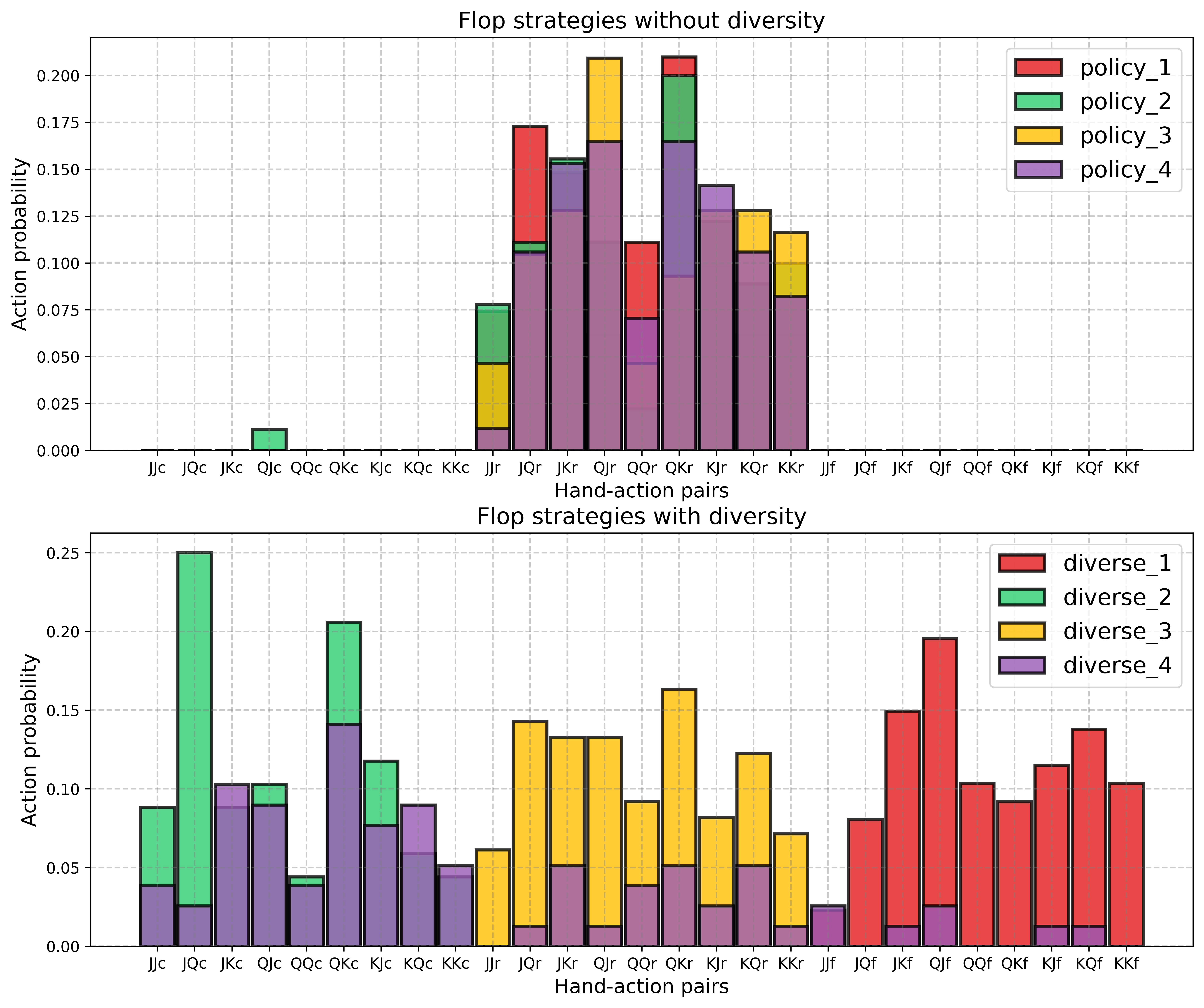
In this section, we verify whether our proposed diversity-regularized policy optimization algorithm can effectively generate policies with different styles. In Leduc poker, hand-action pairs represent different combinations of hands and actions. In the pre-flop phase, each player’s hand has three possibilities, i.e., J, Q, and K. Meanwhile, each player also has three optional actions, i.e., Call (c), Rise (r), and Fold (f). For example, ‘Jc’ means to call when getting the jack. Fig. 3 shows that without the MMD regularization term, the generated strategies have similar styles. By optimizing with the MMD term, the generated strategies are diverse enough which cover a wide range of different states and actions.
4.3.2 Effects of the Hard-OSG and the Diverse-OSG
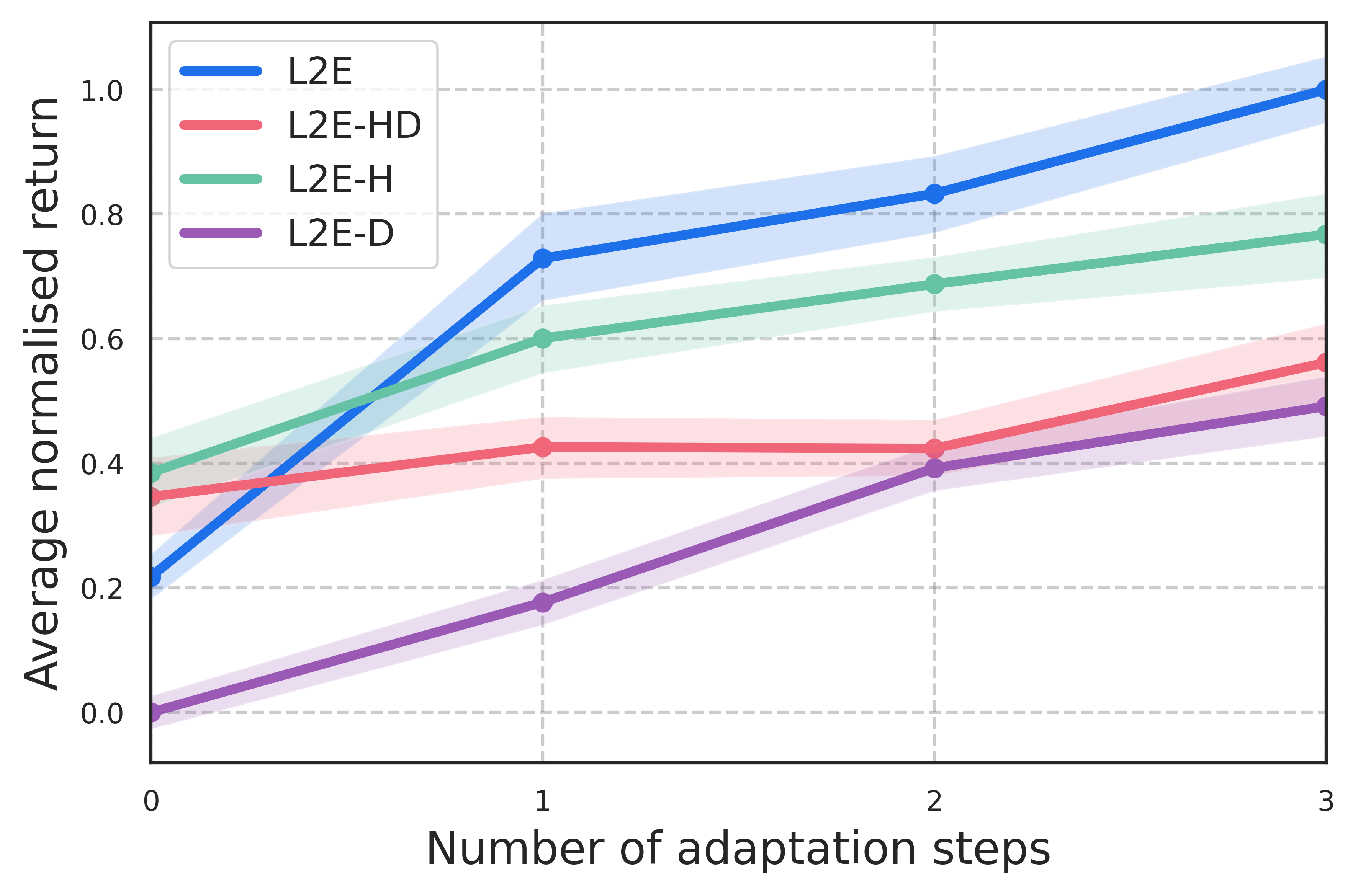
As discussed previously, a crucial step in L2E is the automatic generation of training opponents. The Hard-OSG and Diverse-OSG modules are used to generate opponents that are difficult to exploit and diverse in styles. Fig. 4 shows each module’s impact on the performance, ‘L2E-H’ is L2E without the Hard-OSG module, ‘L2E-D’ is L2E without the Diverse-OSG module, and ‘L2E-HD’ removes both modules altogether. The results show that both Hard-OSG and Diverse-OSG have a crucial influence on L2E’s performance. It is clear that the Hard-OSG module helps to enhance the stability of the base policy, and the Diverse-OSG module can improve the base policy’s performance significantly. Specifically, the performance of ‘L2E-HD’ is unstable, e.g., its two-step adaptation performance is roughly the same as its one-step adaptation performance. ‘L2E-H’ alleviates this problem, but its final performance is still worse than L2E, and the improvement eventually reaches a plateau. With the addition of Hard-OSG, L2E achieves the best performance, and the improvement is faster and more stable. To further demonstrate the generalization ability of L2E, we conducted a series of additional experiments on the BigLeduc poker and the Grid Soccer game environment (see Appendix D and E for more details).
4.4 Convergence Analysis and the Relationship with Nash Equilibrium
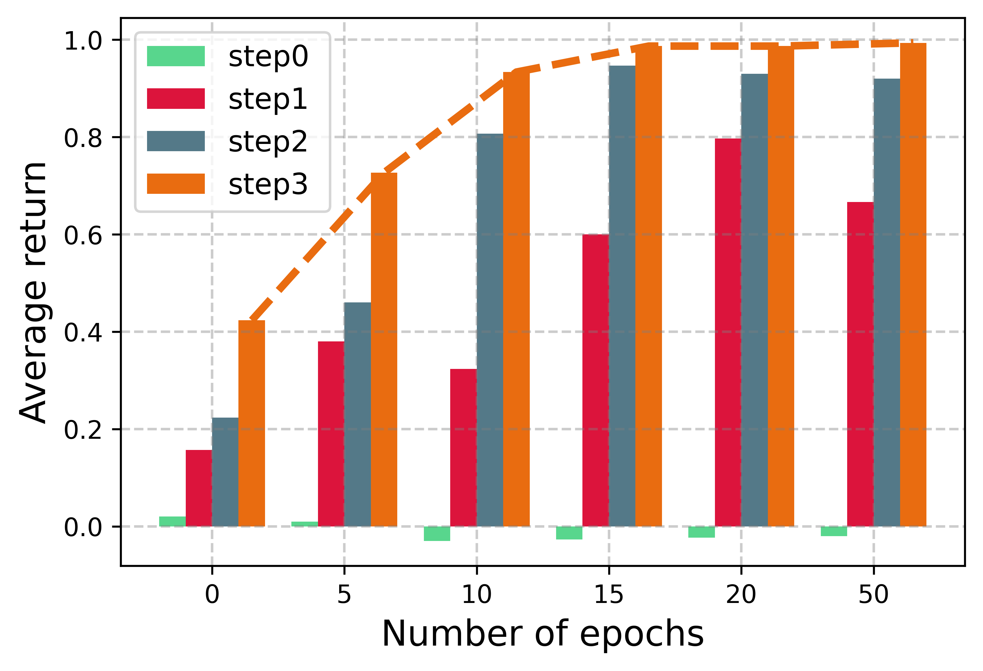
One may wonder whether L2E is supposed to converge at all. If L2E can converge, what is the relationship between the obtained base policy and the equilibrium concepts, such as Nash equilibrium? Since convergence is difficult to analyze theoretically in game theory, we have designed a series of small-scale experiments to empirically analyze L2E’s convergence properties using the Rock-Paper-Scissors (RPS) game. There are several reasons why RPS is chosen: 1) RPS’s strategies are easy to visualize and analyze thanks to the small state and action spaces. 2) RPS’s Nash equilibrium222Choosing Rock, Paper or Scissors with equal probability. is obvious and unique. 3) RPS is often used in game theory for theoretical analysis. From the experimental results in Fig. 5, it can be seen that as the training progresses, L2E’s adaptability becomes stronger and stronger. After reaching a certain number of iterations, the improvement eventually reaches a plateau, which provides some empirical evidence for the convergence of L2E. Similar performance convergence curves can also be observed in the Leduc poker, the BigLeduc poker, and the Grid Soccer environments.
The left side of Fig. 6 visualizes L2E’s trained base policy, i.e., the blue point in the triangle. It is clear that the base policy does not converge to the Nash equilibrium (i.e., the exact center of the triangle) but converges to its vicinity. The orange dot represents the opponent who always chooses Rock. The base policy can exploit this opponent with three steps of gradient update and quickly converge to the best response strategy (i.e., always choose Paper). The right side of Fig. 6 shows that if we set the base policy to the Nash strategy by imitation learning, this Nash base policy (i.e., the star in the triangle) is difficult to adapt to its opponent quickly. From these results, it is clear that L2E’s base policy can adapt to the opponents more quickly than the Nash base policy. This phenomenon is easy to explain. L2E’s base policy is explicitly trained such that a few interactions with a new opponent will produce an opponent-specific policy to exploit this opponent effectively. In contrast, the Nash base policy is essentially a random strategy in this example. Therefore, this vanilla random policy without explicitly trained to fast adapt to its opponents cannot do so. Of course, the Nash base policy can finally converge to its opponent’s best response strategy. But it is much slower than L2E’s base policy.
5 Conclusion
We propose a Learning to Exploit (L2E) framework to exploit sub-optimal opponents without building explicit opponent models. L2E acquires the ability to exploit opponents by a few interactions with different opponents during training to adapt to new opponents during testing quickly. We propose a novel opponent strategy generation algorithm that produces challenging and diverse training opponents for L2E automatically. Detailed experimental results in three challenging environments demonstrate the effectiveness of the proposed L2E framework.
References
- Abdullah et al. (2019) Abdullah, M. A., Ren, H., Ammar, H. B., Milenkovic, V., Luo, R., Zhang, M., and Wang, J. Wasserstein robust reinforcement learning. arXiv preprint arXiv:1907.13196, 2019.
- Agapitos et al. (2008) Agapitos, A., Togelius, J., Lucas, S. M., Schmidhuber, J., and Konstantinidis, A. Generating diverse opponents with multiobjective evolution. In IEEE Symposium On Computational Intelligence and Games, pp. 135–142, 2008.
- Al-Shedivat et al. (2018) Al-Shedivat, M., Bansal, T., Burda, Y., Sutskever, I., Mordatch, I., and Abbeel, P. Continuous adaptation via meta-learning in nonstationary and competitive environments. In International Conference on Learning Representations, 2018.
- Albrecht & Stone (2017) Albrecht, S. V. and Stone, P. Reasoning about hypothetical agent behaviours and their parameters. In International Conference on Autonomous Agents and Multiagent Systems, pp. 547–555, 2017.
- Albrecht & Stone (2018) Albrecht, S. V. and Stone, P. Autonomous agents modelling other agents: A comprehensive survey and open problems. Artificial Intelligence, 258:66–95, 2018.
- Banerjee & Sen (2007) Banerjee, D. and Sen, S. Reaching pareto-optimality in prisoner’s dilemma using conditional joint action learning. Autonomous Agents and Multi-Agent Systems, 15(1):91–108, 2007.
- Brown (1951) Brown, G. W. Iterative solution of games by fictitious play. Activity Analysis of Production and Allocation, 13(1):374–376, 1951.
- de Weerd et al. (2017) de Weerd, H., Verbrugge, R., and Verheij, B. Negotiating with other minds: the role of recursive theory of mind in negotiation with incomplete information. Autonomous Agents and Multi-Agent Systems, 31(2):250–287, 2017.
- Dekel et al. (2004) Dekel, E., Fudenberg, D., and Levine, D. K. Learning to play bayesian games. Games and Economic Behavior, 46(2):282–303, 2004.
- Eysenbach et al. (2018) Eysenbach, B., Gupta, A., Ibarz, J., and Levine, S. Diversity is all you need: Learning skills without a reward function. In International Conference on Learning Representations, 2018.
- Finn et al. (2017) Finn, C., Abbeel, P., and Levine, S. Model-agnostic meta-learning for fast adaptation of deep networks. In International Conference on Machine Learning, pp. 1126–1135, 2017.
- Foerster et al. (2018) Foerster, J., Chen, R. Y., Al-Shedivat, M., Whiteson, S., Abbeel, P., and Mordatch, I. Learning with opponent-learning awareness. In International Conference on Autonomous Agents and MultiAgent Systems, pp. 122–130, 2018.
- Fortunato et al. (2018) Fortunato, M., Azar, M. G., Piot, B., Menick, J., Hessel, M., Osband, I., Graves, A., Mnih, V., Munos, R., Hassabis, D., et al. Noisy networks for exploration. In International Conference on Learning Representations, 2018.
- Fukumizu et al. (2009) Fukumizu, K., Gretton, A., Lanckriet, G. R., Schölkopf, B., and Sriperumbudur, B. K. Kernel choice and classifiability for rkhs embeddings of probability distributions. In Advances in Neural Information Processing Systems, pp. 1750–1758, 2009.
- Gretton et al. (2007) Gretton, A., Borgwardt, K., Rasch, M., Schölkopf, B., and Smola, A. J. A kernel method for the two-sample-problem. In Advances in Neural Information Processing Systems, pp. 513–520, 2007.
- Gretton et al. (2012) Gretton, A., Borgwardt, K. M., Rasch, M. J., Schölkopf, B., and Smola, A. A kernel two-sample test. The Journal of Machine Learning Research, 13(1):723–773, 2012.
- Grosz & Sidner (1986) Grosz, B. and Sidner, C. L. Attention, intentions, and the structure of discourse. Computational Linguistics, 1986.
- Gupta et al. (2018) Gupta, A., Eysenbach, B., Finn, C., and Levine, S. Unsupervised meta-learning for reinforcement learning. arXiv preprint arXiv:1806.04640, 2018.
- He et al. (2016) He, H., Boyd-Graber, J., Kwok, K., and Daumé III, H. Opponent modeling in deep reinforcement learning. In International Conference on Machine Learning, pp. 1804–1813, 2016.
- Hospedales et al. (2020) Hospedales, T., Antoniou, A., Micaelli, P., and Storkey, A. Meta-learning in neural networks: A survey. arXiv preprint arXiv:2004.05439, 2020.
- Huynh et al. (2006) Huynh, T. D., Jennings, N. R., and Shadbolt, N. R. An integrated trust and reputation model for open multi-agent systems. Autonomous Agents and Multi-Agent Systems, 13(2):119–154, 2006.
- Jaderberg et al. (2017) Jaderberg, M., Dalibard, V., Osindero, S., Czarnecki, W. M., Donahue, J., Razavi, A., Vinyals, O., Green, T., Dunning, I., Simonyan, K., et al. Population based training of neural networks. arXiv preprint arXiv:1711.09846, 2017.
- Jaderberg et al. (2019) Jaderberg, M., Czarnecki, W. M., Dunning, I., Marris, L., Lever, G., Castaneda, A. G., Beattie, C., Rabinowitz, N. C., Morcos, A. S., Ruderman, A., et al. Human-level performance in 3d multiplayer games with population-based reinforcement learning. Science, 364(6443):859–865, 2019.
- Jarvis et al. (2005) Jarvis, P. A., Lunt, T. F., and Myers, K. L. Identifying terrorist activity with ai plan recognition technology. AI Magazine, 26(3):73–73, 2005.
- Lanctot et al. (2017) Lanctot, M., Zambaldi, V., Gruslys, A., Lazaridou, A., Tuyls, K., Pérolat, J., Silver, D., and Graepel, T. A unified game-theoretic approach to multiagent reinforcement learning. In Advances in Neural Information Processing Systems, pp. 4190–4203, 2017.
- McCalla et al. (2000) McCalla, G., Vassileva, J., Greer, J., and Bull, S. Active learner modelling. In International Conference on Intelligent Tutoring Systems, pp. 53–62, 2000.
- Mealing & Shapiro (2015) Mealing, R. and Shapiro, J. L. Opponent modeling by expectation–maximization and sequence prediction in simplified poker. IEEE Transactions on Computational Intelligence and AI in Games, 9(1):11–24, 2015.
- Muise et al. (2015) Muise, C., Belle, V., Felli, P., McIlraith, S., Miller, T., Pearce, A. R., and Sonenberg, L. Planning over multi-agent epistemic states: A classical planning approach. In AAAI Conference on Artificial Intelligence, pp. 3327–3334, 2015.
- Nachbar (2005) Nachbar, J. H. Beliefs in repeated games. Econometrica, 73(2):459–480, 2005.
- Nichol et al. (2018) Nichol, A., Achiam, J., and Schulman, J. On first-order meta-learning algorithms. arXiv preprint arXiv:1803.02999, 2018.
- Pattanaik et al. (2018) Pattanaik, A., Tang, Z., Liu, S., Bommannan, G., and Chowdhary, G. Robust deep reinforcement learning with adversarial attacks. In International Conference on Autonomous Agents and MultiAgent Systems, pp. 2040–2042, 2018.
- Pinto et al. (2017) Pinto, L., Davidson, J., Sukthankar, R., and Gupta, A. Robust adversarial reinforcement learning. In International Conference on Machine Learning, pp. 2817–2826, 2017.
- Plappert et al. (2018) Plappert, M., Houthooft, R., Dhariwal, P., Sidor, S., Chen, R. Y., Chen, X., Asfour, T., Abbeel, P., and Andrychowicz, M. Parameter space noise for exploration. In International Conference on Learning Representations, 2018.
- Powers & Shoham (2005) Powers, R. and Shoham, Y. Learning against opponents with bounded memory. In International Joint Conference on Artificial Intelligence, pp. 817–822, 2005.
- Rabinowitz et al. (2018) Rabinowitz, N., Perbet, F., Song, F., Zhang, C., Eslami, S. A., and Botvinick, M. Machine theory of mind. In International Conference on Machine Learning, pp. 4218–4227, 2018.
- Schulman et al. (2015) Schulman, J., Levine, S., Abbeel, P., Jordan, M., and Moritz, P. Trust region policy optimization. In International Conference on Machine Learning, pp. 1889–1897, 2015.
- Shapley (1953) Shapley, L. S. Stochastic games. Proceedings of the National Academy of Sciences, 39(10):1095–1100, 1953.
- Sriperumbudur et al. (2010) Sriperumbudur, B. K., Fukumizu, K., Gretton, A., Schölkopf, B., and Lanckriet, G. R. Non-parametric estimation of integral probability metrics. In IEEE International Symposium on Information Theory, pp. 1428–1432, 2010.
- Steinberger (2019) Steinberger, E. Single deep counterfactual regret minimization. arXiv preprint arXiv:1901.07621, 2019.
- Sukthankar & Sycara (2007) Sukthankar, G. and Sycara, K. Policy recognition for multi-player tactical scenarios. In International Joint Conference on Autonomous Agents and Multiagent Systems, pp. 1–8, 2007.
- Synnaeve & Bessiere (2011) Synnaeve, G. and Bessiere, P. A Bayesian model for opening prediction in rts games with application to StarCraft. In IEEE Conference on Computational Intelligence and Games, pp. 281–288, 2011.
- Vinyals et al. (2019) Vinyals, O., Babuschkin, I., Czarnecki, W. M., Mathieu, M., Dudzik, A., Chung, J., Choi, D. H., Powell, R., Ewalds, T., Georgiev, P., et al. Grandmaster level in StarCraft II using multi-agent reinforcement learning. Nature, 575(7782):350–354, 2019.
- Wang et al. (2016) Wang, J. X., Kurth-Nelson, Z., Tirumala, D., Soyer, H., Leibo, J. Z., Munos, R., Blundell, C., Kumaran, D., and Botvinick, M. Learning to reinforcement learn. arXiv preprint arXiv:1611.05763, 2016.
- Wang et al. (2019) Wang, R., Lehman, J., Clune, J., and Stanley, K. O. Paired open-ended trailblazer (poet): Endlessly generating increasingly complex and diverse learning environments and their solutions. arXiv preprint arXiv:1901.01753, 2019.
- Weber & Mateas (2009) Weber, B. G. and Mateas, M. A data mining approach to strategy prediction. In IEEE Symposium on Computational Intelligence and Games, pp. 140–147, 2009.
- Wen et al. (2018) Wen, Y., Yang, Y., Luo, R., Wang, J., and Pan, W. Probabilistic recursive reasoning for multi-agent reinforcement learning. In International Conference on Learning Representations, 2018.
- Xu et al. (2018) Xu, Z., van Hasselt, H. P., and Silver, D. Meta-gradient reinforcement learning. In Advances in Neural Information Processing Systems, pp. 2396–2407, 2018.
- Zinkevich et al. (2008) Zinkevich, M., Johanson, M., Bowling, M., and Piccione, C. Regret minimization in games with incomplete information. In Advances in Neural Information Processing Systems, pp. 1729–1736, 2008.
Appendices
Appendix A Maximum Mean Discrepancy
We use the Maximum Mean Difference (MMD) (Gretton et al., 2007) metric to measure the differences between the distributions of trajectories induced by different opponent strategies. In contrast to the Wasserstein distance and Dudley metrics, the MMD metric has closed-form solutions. Furthermore, unlike KL-divergence, the MMD metric is strongly consistent while exhibiting good rates of convergence (Sriperumbudur et al., 2010).
Definition 1 Let be a function space . Suppose we have two distributions and , , . The MMD between and using test functions from the function space is defined as follows:
| (15) |
By picking a suitable function space , we get the following important theorem (Gretton et al., 2007).
Theorem 1 Let be a unit ball in a Reproducing Kernel Hilbert Space (RKHS). Then if and only if .
is a feature space mapping from to RKHS, we can easily calculate the MMD distance using the kernel method :
| (16) |
The expectation terms in Eq. (16) can be approximated using samples:
| (17) |
The gradient of the MMD term with respect to the policy’s parameter
| (18) |
where is the probability of the trajectory. Since , is the known opponent policy that has no dependence on . The gradient with respect to the parameters in first term is 0. The gradient of the second and third terms can be easily calculated as follows:
| (19) |
Appendix B Algorithm
B.1 Hard-OSG
Alg. 2 is the overall description of the hard-to-exploit training opponent generation algorithm.
| (20) |
| (21) |
| (22) |
| (23) |
B.2 Diverse-OSG
Alg. 3 is the overall description of the diverse training opponent generation algorithm.
| (24) |
B.3 L2E’s testing procedure
Alg. 4 is the testing procedure of our L2E framework.
| (25) |
Appendix C Leduc Poker
The Leduc poker generally uses a deck of six cards that includes two suites, each with three ranks (Jack, Queen, and King of Spades, Jack, Queen, and King of Hearts). The game has a total of two rounds. Each player is dealt with a private card in the first round, with the opponent’s deck information hidden. In the second round, another card is dealt with as a community card, and the information about this card is open to both players. If a player’s private card is paired with the community card, that player wins the game; otherwise, the player with the highest private card wins the game. Both players bet one chip into the pot before the cards are dealt. Moreover, a betting round follows at the end of each dealing round. The betting wheel alternates between two players, where each player can choose between the following actions: call, check, raise, or fold. If a player chooses to call, that player will need to increase his bet until both players have the same number of chips. If one player raises, that player must first make up the chip difference and then place an additional bet. Check means that a player does not choose any action on the round but can only check if both players have the same chips. If a player chooses to fold, the hand ends, and the other player wins the game. When all players have equal chips for the round, the game moves on to the next round. The final winner wins all the chips in the game.
Next, we introduce how to define the state vector. Position in a poker game is a critical piece of information that determines the order of action. We define the button (the pre-flop first-hand position), the action position (whose turn it is to take action), and the current game round as one dimension of the state, respectively. In Poker, the combination of a player’s hole cards and board cards determines the game’s outcome. We encode the hole cards and the board cards separately. The amount of chips is an essential consideration in a player’s decision-making process. We encode this information into two dimensions of the state. The number of chips in the pot can reflect the action history of both players. The difference in bets between players in this round affects the choice of action (the game goes to the next round until both players have the same number of chips). In summary, the state vector has seven dimensions, i.e., button, to_act, round, hole cards, board cards, chips_to_call, and pot.
Appendix D BigLeduc Poker
We use a larger and more challenging BigLeduc poker environment to further verify the effectiveness of our L2E framework. The BigLeduc poker has the same rules as Leduc but uses a deck of 24 cards with 12 ranks. In addition to the larger state space, BigLeduc allows a maximum of 6 instead of 2 raises per round. As shown in Fig. 7, L2E still achieves fast adaptation to different opponents. In comparison with other baseline methods, L2E achieves the highest average return in Table 2.
| Random | Call | Raise | Oracle | |
|---|---|---|---|---|
| L2E | 0.820.28 | 0.740.22 | 0.680.09 | -1.020.24 |
| MAML | 0.770.30 | 0.170.08 | -2.020.99 | -1.210.30 |
| Random | -0.003.08 | -0.002.78 | -2.835.25 | -1.884.28 |
| TRPO | 0.190.09 | 0.100.16 | -2.220.71 | -1.420.47 |
| TRPO-P | 0.360.42 | 0.230.21 | -2.031.61 | -1.690.69 |
| EOM | 0.560.43 | 0.150.13 | -1.150.12 | -1.630.62 |
Appendix E Grid Soccer
This game contains a board with a grid, two players, and their respective target areas. The position of the target area is fixed, and the two players appear randomly in their respective areas at the start of the game. One of the two players randomly has the ball. The goal of all players is to move the ball to the other player’s target position. When the two players move to the same grid, the player with the ball loses the ball. Players gain one point for moving the ball to the opponent’s area. The player can move in all four directions within the grid, and action is invalid when it moves to the boundary.
We train the L2E algorithm in this soccer environment in which both players are modeled by a neural network. Inputs to the network include information about the position of both players, the position of the ball, and the boundary. We provide two types of opponents to test the effectiveness of the resulting base policy. 1) A defensive opponent who adopts a strategy of not leaving the target area and preventing opposing players from attacking. 2) An aggressive opponent who adopts a strategy of continually stealing the ball and approaching the target area with the ball. Facing a defensive opponent will not lose points, but the agent must learn to carry the ball and avoid the opponent moving to the target area to score points. Against an aggressive opponent, the agent must learn to defend at the target area to avoid losing points. Fig. 8 shows the comparisons between L2E, MAML, and TRPO. L2E adapts quickly to both types of opponents; TRPO works well against defensive opponents but loses many points against aggressive opponents; MAML is unstable due to its reliance on task specification during the training process.
Appendix F Hyper-parameters
The hyper-parameters of all experiments are shown in the table below.
| Hyper-parameter | Value |
| Training step size hyper parameters | (0.1,0.01) |
| Testing step size hyper parameter | 0.1 |
| Number of opponents sampled per batch | 40 |
| Number of trajectories to sample for each opponent | 20 |
| Number of gradient steps in the training loop | 1 |
| Number of gradient steps in the testing loop | 3 |
| Policy network size(Leduc, BigLeduc, Grid Soccer) | [64,64,(4,4,5)] |
| Number of training steps required for convergence in Leduc | 300 |
| Number of training steps required for convergence in BigLeduc | 400 |
| Number of training steps required for convergence in GridSoccer | 300 |
| Hard-to-exploit opponent training epochs | 20 |
| Diverse opponent training epochs | 50 |
| Weight of the MMD term | 0.8 |
| Bandwidth of RBF kernel | 1 |
| Minimum trajectory length N to calculate MMD term | 20 |
| Number of opponent strategies generated by OSG per round of iteration | N5 |
| Number of trajectories sampled to compute MMD term | 8 |