HVAQ: A High-Resolution Vision-Based Air Quality Dataset

Abstract

Air pollutants, such as particulate matter, negatively impact human health. Most existing pollution monitoring techniques use stationary sensors, which are typically sparsely deployed. However, real-world pollution distributions vary rapidly with position and the visual effects of air pollution can be used to estimate concentration, potentially at high spatial resolution. Accurate pollution monitoring requires either densely deployed conventional point sensors, at-a-distance vision-based pollution monitoring, or a combination of both.

The main contribution of this paper is that to the best of our knowledge, it is the first publicly available, high temporal and spatial resolution air quality dataset containing simultaneous point sensor measurements and corresponding images. The dataset enables, for the first time, high spatial resolution evaluation of image-based air pollution estimation algorithms. It contains PM2.5, PM10, temperature, and humidity data. We evaluate several state-of-art vision-based PM concentration estimation algorithms on our dataset and quantify the increase in accuracy resulting from higher point sensor density and the use of images. It is our intent and belief that this dataset can enable advances by other research teams working on air quality estimation. Our dataset is available at https://github.com/implicitDeclaration/HVAQ-dataset/tree/master.

I Introduction

Air pollution is a serious threat to human health, and is closely related to disease and death rates [1, 2, 3, 4, 5]. According to the World Health Organization (WHO), air pollution causes seven million premature deaths per year, largely as a result of increased mortality from stroke, heart disease, and lung cancer. The most common harmful air pollutants are particulate matter (PM), sulfur dioxide, and nitrogen dioxide. This work focuses on PM, which can increase the rate of cardiovascular and respiratory diseases [6, 7].

Air monitoring stations are mainly used to obtain air pollution data [8]. However, air pollution concentration can vary within a relatively short distance: the low sensor density (see Figure 1) can lead to inaccurate estimation of the high-resolution pollution field. Low measurement spatial density makes it especially difficult to estimate human exposure to air pollution.

The PM concentrations are correlated with source distributions. For example, PM has heterogeneous sources [9], e.g., automobiles, manufacturing, and building construction etc. In addition, numerous factors, including wind, humidity, and geography [10, 11], are related to PM distributions. Increasing sensor density or adding image sensors supporting high spatial resolution captures can increase the field estimation accuracy and resolution of pollutant concentrations.

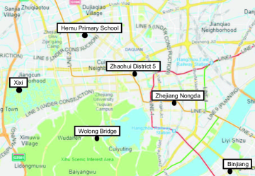
Figure 1: The distribution of air monitoring stations in Hangzhou. On average, there is one monitoring site for every 35 square kilometers.

In addition to air quality sensors, image sensors can also be used to estimate PM concentrations, potentially at higher spatial resolutions [12, 13]. Image data can be derived from several sources such as social media and digital cameras [14, 15]. Moreover, consumer-grade cameras are inexpensive and can gather pollution data over a wide field of view (see Figure  2). PM can be estimated by analyzing the visual haze effect caused by scattering and absorption [13]. On days with high pollution,visibility is low because light is scattered away from the camera by PM.

The ground truth pollution data are typically obtained from the nearest of several sparsely deployed monitoring stations. Lack of high-resolution ground truth pollution measurements makes it difficult to evaluate vision-based pollution estimation techniques, as pollution can vary rapidly with position [15]. Moreover, vision-based pollution estimation techniques generally assume homogeneous distributions of particles and gases within images, implying constant light attenuation [15]. In reality, pollution concentration changes rapidly in space. Therefore, accurate evaluation of vision-based estimation algorithms requires high-resolution datasets [16].

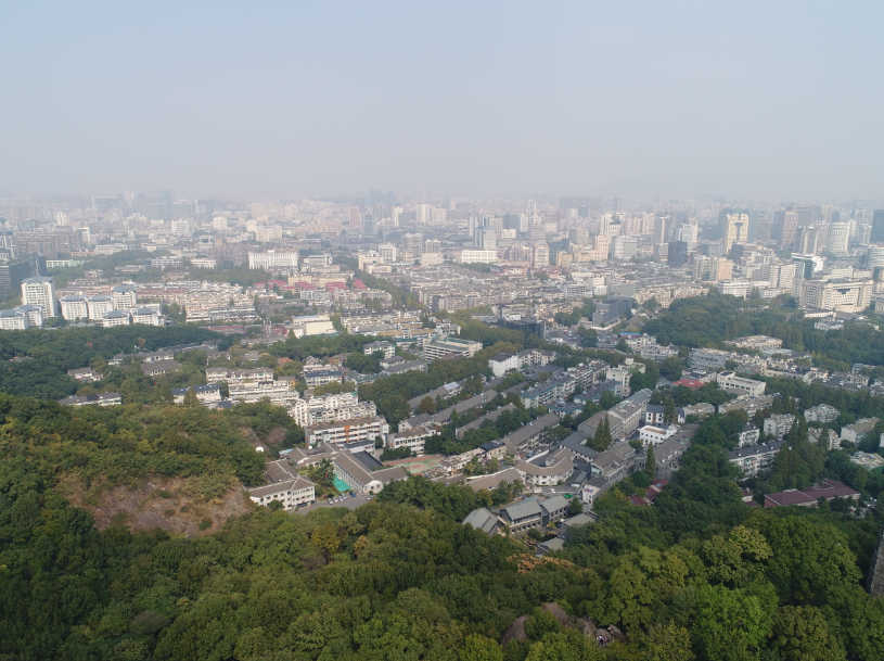
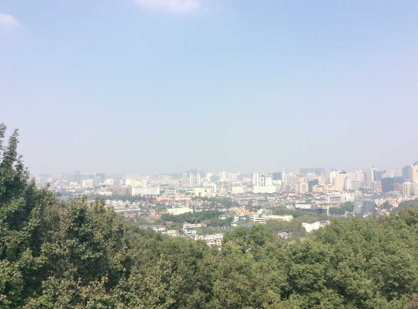
Figure 2: (a) High altitude quadcopter view and (b) low altitude camera view.

This paper presents a dataset containing high spatial (one sensor every 2.5 square kilometers) and temporal (one second interval) resolution particle counter based pollution measurements with corresponding images, in addition to auxiliary information including GPS locations, humidity, and temperature. These properties are significant: this is the first publicly available dataset capable of being used to train and evaluate vision-based pollution estimation and forecasting techniques at high spatial resolutions. To the best of our knowledge, there have been no publicly available datasets enabling evaluation in this context. Certainly, There are datasets containing high-resolution [16, 17] and wide coverage [18, 19] air pollution data. However, none of them contain corresponding synchronized images. Based on the dataset, which is the primary contribution of this paper, we also make several observations, e.g., the rate of spatial variation in pollution concentration and the evaluation of several existing vision-based PM concentration predication algorithms. To evaluate the improvement brought by increasing sensor spatial resolution and using images, we use heterogeneous information for concentration estimation, i.e., images and particle counter based PM concentrations, which were not considered in the previous vision-based algorithms.

The rest of the paper is organized as follows. Section II summarizes related work. Sections III and IV describe our data collection and analysis process. Section V presents the experimental results. Section VI concludes the paper.

II Related Work

The related work can be generalized into three categories: environment monitoring methods, spectrum RGB cameras, and vision-based techniques, respectively.

TABLE I: Datasets comparison.

	Spatial	Temporal	Scale	Images
	resolution	resolution
Apte et al.	High	Second	$30\text{\,}{\mathrm{km}}^{2}$	No
ChinaHighPM10	Low	Hour	9.6M$\text{\,}{\mathrm{km}}^{2}$	No
ImgSensingNet	High	Hour	$7\text{\,}{\mathrm{km}}^{2}$	Yes
Air monitoring	Low	Hour	$16\,853\text{\,}{\mathrm{km}}^{2}$	No
stations (Hangzhou)
HVAQ	High	Second	$1\text{\,}{\mathrm{km}}^{2}$	Yes

II-A Environment Monitoring Methods

Most existing air quality monitoring systems [20] have low temporal and spatial resolutions. For example, Janssens-Maenhout et al. [21] provide a harmonized gridded air pollution emission dataset. This dataset includes multiple pollutants on a global scale with $0.1^{\circ}\times 0.1^{\circ}$ spatial resolution (latitude and longitude). De et al. [22] collect an air quality dataset containing 9,358 instances of hourly averaged responses from metal oxide chemical sensors. Devices are deployed in a highly polluted area in Italy at high spatial resolution. Li et al. [23] provide a dataset of mobile air quality measurements in Zurich. They use sensor boxes installed on mobile trams. Static installations are also deployed close to high-quality reference stations for calibration. Their sensors move around the city, recording every $5\text{\,}\mathrm{s}$. Apte et al. [16] use two Google street view vehicles equipped with data acquisition platforms to collect the air pollution data of a $30\text{\,}{\mathrm{km}}^{2}$ city area. Their data contains nitrogen oxides and black carbon. Unlike our dataset, it does not contain PM concentrations, images, and weather conditions. Wei et al. [18] describe the ChinaHighPM10 dataset, which integrates multiple data sources and contains hourly PM10 data in China with $1\text{\,}\mathrm{km}$ resolution. Generally, these datasets typically do not include images for the evaluation of vision-based pollution estimation.

Yang et al. [24] describe ImgSensingNet, an air quality monitoring system consisting of unmanned-aerial-vehicles (UAV) and ground sensors. Their system uses UAVs for vision-based air quality index (AQI) monitoring and activates the ground sensing network based on vision-based AQI inference. Their dataset differs from ours as follows. (1) It is not public nor can be expected to be public in the near future. (2) Their data have time gaps, i.e., there is ground sensor data only when the UAV is uncertain about the AQI in some areas, making the intervals without ground sensor data useless for validating vision-based algorithms. In contrast, our data acquisition system operated continuously. (3) Their dataset contains an irreversible AQI index inferred from PM data, while our dataset provides raw PM data, meteorology information, and environmental information. (4) Their point sensor data acquisition period is one hour (at best, depending on whether the point sensors are activated) while ours is one second. Table I compares different datasets. Our HVAQ is unique in providing high spatial and temporal resolution pollution measurements with corresponding images. Moreover, it has been publicly released.

II-B Spectrum-Based RGB Cameras

Image data are typically gathered using spectral measurements, imaging systems, and multi-spectral imaging [25]. Spectral measurements acquire accurate color data without structural information from the scene. Imaging systems such as scanners or digital RGB cameras capture detailed structural information [26] with a limited number of color channels. Mismatches between the camera’s spectral sensitivities and desired color matching functions can reduce the camera’s color quality.

In contrast, multi-spectral imaging can produce accurate, detailed representations of the scene for both color and structure [27]. Nonetheless, multi-spectral imaging systems are expensive, while spectral measurements provide very limited spatial resolution.

II-C Image-based Techniques

Vision-based pollution estimation is being studied due to its spatial range and low cost. Li et al. [14] analyze photos acquired from social media and establish the correlation between visual haze and PM2.5 concentration. Liu et al. [15] estimate PM2.5 using support vector regression on six features extracted from images. Zhang et al. [12] describe an air pollution estimation algorithm that uses outdoor photos. They use a convolutional neural network to predict the pollution level. Rijal et al. [28] integrate the prediction of multiple neural networks to calculate the PM2.5 of images. The ensemble of neural networks provides more accurate estimation than a single network. Gu et al. [29] designed a vision-based estimation of PM2.5 concentration. It requires low-pollution reference images for each area of interest. Zhang et al. [13] estimate multiple pollution concentrations from images using scattering and absorption models.

The main problem is that it is unclear how accurate these methods are because, until now, ground-truth data are of very low spatial resolution. Therefore, our dataset makes it possible to evaluate them in a high-resolution scenario.

TABLE II: GPS Locations of Our Sensors and Picture.

Location	P1	P2	P3
Longitude	$120.153173^{\circ}$	$120.15488^{\circ}$	$120.153894^{\circ}$
Latitude	$30.269884^{\circ}$	$30.268726^{\circ}$	$30.27096^{\circ}$
P4	P5	P6	P7
$120.156252^{\circ}$	$120.153905^{\circ}$	$120.15936^{\circ}$	$120.155162^{\circ}$
$30.270242^{\circ}$	$30.27358^{\circ}$	$30.273139^{\circ}$	$30.278369^{\circ}$
P8	P9	P10	Photo location
$120.161912^{\circ}$	$120.164792^{\circ}$	$120.156541^{\circ}$	$120.153955^{\circ}$
$30.276465^{\circ}$	$30.279437^{\circ}$	$30.283932^{\circ}$	$30.267191^{\circ}$

TABLE III: Pairwise Sensors Distance (m).

	P1	P2	P3	P4	P5	P6	P7	P8	P9	P10
P1	0	113	168	281	464	697	1012	1150	1730	1625
P2		0	211	190	509	603	1040	1089	1537	1660
P3			0	245	296	575	844	1000	1450	1457
P4				0	388	413	871	899	1347	1510
P5					0	464	548	819	1250	1161
P6						0	625	486	934	1170
P7							0	656	918	613
P8								0	448	953
P9									0	877
P10										0

III Sensor Deployment

This section describes the deployment of our sensors and cameras in order to collect both high-resolution ground-truth data and corresponding images.

III-A Sensor Calibration

Our sensing platform is equipped with humidity and temperature sensors. The precision is 3% relative humidity (RH) and $\pm$$0.3\text{\,}\mathrm{\SIUnitSymbolCelsius}$, respectively. The PM sensor model is Nova SDS011, which can detect particles with $0.3\text{\,}\mathrm{\SIUnitSymbolMicro m}$ to $10\text{\,}\mathrm{\SIUnitSymbolMicro m}$ diameters according to the scattered light intensity in a specific direction [30].

We calibrated our particle counting sensors based on the measurements from the air quality monitoring site of Hangzhou Meteorological Bureau in Hemu Primary School using co-location method [31]. Our device is co-located with an air monitoring station, which is equipped with a high-precision sensor. The device collects data for 58 hours continuously. The station data are considered ground truth. We use the least-squares method to fit a quadratic function to the ground truth data. According to the measured concentration, we fit the data into a two-stage piecewise linear function. The fitted function is as follows.

$$y=\begin{cases}1.61x+16.01&\text{for }0\leqslant x\leqslant 30\text{ and}\\ 0.13x+29.48&\text{for }x>30,\\ \end{cases}$$ (1)

where $x$ is the original value and $y$ is the calibrated one. The calibration data are gathered during a 2 day period and the result is shown in Figure 3. Calibration reduces root mean squared error from $32.74\text{\,}\mathrm{\SIUnitSymbolMicro g}\text{\,}{\mathrm{m}}^{-3}$ to $3.88\text{\,}\mathrm{\SIUnitSymbolMicro g}\text{\,}{\mathrm{m}}^{-3}$, while the variance for all the data over all locations is $9.33\text{\,}\mathrm{\SIUnitSymbolMicro g}\text{\,}{\mathrm{m}}^{-3}$.

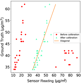
Figure 3: Pollution concentration calibration.

III-B Deployment Details

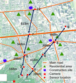
Figure 4: The distribution of sensors and pollution sources. Sensor locations are numbered in ascending order according to the distance from the camera.

Our dataset contains both high-resolution ground truth data and wide-view images. The sensors are placed outdoors and close to living areas. The city center is very crowded and the air quality here affects people more significantly. We deploy our sensors in the urban area of Hangzhou, a city of more than 8 million residents and frequently affected by high PM2.5 concentrations [32]. Existing research [33] shows that in the main urban area of Hangzhou, the sources of PM2.5 are biomass burning/construction dust (41.6%), vehicle exhaust/metallurgical (metals’ production and purification) dust (29.3%), unknown source (11.2%), oil combustion (9.8%), and soil (8.0%). As shown in Figure 4, the main pollution sources are marked on the map and the sensors are located on two straight lines from the observation point. The GPS locations and distances between each pair of sensors are listed in Table II and Table III. The sensors are sampled every second and an image is captured every $20\text{\,}\mathrm{m}\mathrm{i}\mathrm{n}\mathrm{u}\mathrm{t}\mathrm{e}\mathrm{s}$. Since the temporal variation of PM concentration is slower than the acquisition rate of the sensors, and the image acquisition rate is also limited by the flight time of quadcopter, images are captured less frequently.

To derive a wide-view image covering all sensor locations, we mount a camera on a quadcopter as shown in Figure 5. We use two approaches to take photos. First, we use a quadcopter equipped with a 4864$\times$3648 camera at $90\text{\,}\mathrm{m}$ altitude. Moreover, since the quadcopter has limited carrying and battery capacities, we also take pictures at a fixed location on the mountain top with a resolution of 2592$\times$1936 using an iPad and at a resolution of 4000$\times$3000 using a phone. The parameters of our cameras are listed in Table V. The quadcopter camera uses the Sony Exmor R CMOS sensor. The other two cameras types are the Apple iSight and Sony IMX586. 106 images and over 300 thousand PM samples were gathered in three days.

Apparently, the cost of vision-based approach (about $30) is much less than the total cost of the sensors (about $670). Thus, predicting air pollution concentrations using images is more convenient and less expensive than particle counters, but requires sophisticated image processing algorithms. Table IV lists our equipment.

TABLE IV: Used equipments.

	Camera	Quadcopter	Sensors	Battery	Platform
Price ($)	200-460	1500	3-15	12	37
Model	Quadcopter default camera, iPad, Onplus 7 phone camera	Dji Phantom 4 Pro	PM2.5, PM10, humidity, temperature	4000 mAh	Raspi 3B+

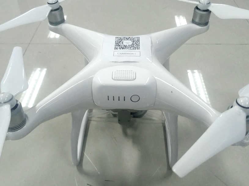
Figure 5: The quadcopter (Dji Phantom 4 Pro) used in our deployment.

TABLE V: Camera Parameter.

Camera	Pixel	Sensor	Aperture
quadcopter	20,000,000	Sony Exmor R	f/2.8-f/11
pad	8,000,000	iSight	f/2.4
phone	48,000,000	Sony IMX586	f/1.6

IV Dataset Analysis

Q1) What is the impact of environmental conditions on measurement accuracy?

Our data collection period spans three days with varying environmental conditions. The impact of the environmental conditions determines the corresponding parameters of the calibration functions. Thus, it is important to investigate the relationship between the impact of environmental conditions on measurement accuracy.

Q2) What are the spatial variation characteristics of PM2.5 concentration?

Since the spatial distribution of PM2.5 determines the required sensor density, this information helps us to determine the benefits of increasing the spatial resolution of a pollution sensor network.

Q3) How does the correlation of pollution concentrations at two different locations depend on their separation?

The relationship between PM2.5 concentration and distance provides information relevant to the required number of sensors. For example, if the PM2.5 concentrations at two locations are highly correlated, one sensor might be used to determine the concentrations at both locations.

Q4) How much do additional point sensors and vision-based methods improve estimation accuracy?

This question builds on Q2 and Q3. To evaluate the effectiveness and novelty of our new air quality dataset, it is important to understand how the sensor density and the use of images relates to the PM2.5 estimation accuracy.

IV-A Temperature and Humidity Correlations with Pollution Concentrations

Environmental factors such as weather conditions can affect sensor readings. For the deployments on Oct. 19 and Nov. 10, we calculate the $R^{2}$ correlation coefficients for PM2.5 and several environmental factors.

A1: Environmental conditions have limited impact. The results in Table VI shows that the correlations between PM2.5 and weather factors are insignificant. Wu et al. [34] report that temperature is not significantly correlated to PM concentrations in Hangzhou and PM2.5 concentration is only significantly elevated when RH is higher than 60%. Moreover, the correlation between environmental factors and PM concentration also depends on the region and season, e.g., Zhu et al. [35] report that PM concentration and RH show seasonal correlation. However, since temperature and humidity do not directly affect the measurement process of particle counters, we do not include temperature and humidity in our calibration functions.

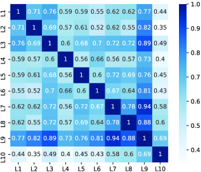
Figure 6: The confusion matrix for PM2.5 correlation. The number on the axis represents the number of the corresponding location.

TABLE VI: PM2.5 Correlation with PM10 and Environmental Factors on Oct. 19 and Nov. 10.

	PM2.5	Temperature	Humidity
PM2.5	1.0	0.298	0.306
Temperature	0.298	1.0	0.808
Humidity	0.306	0.808	1.0

IV-B Correlations of PM Readings

TABLE VII: Statistics for PM and Environmental Data.

Data in Different Days	Standard Deviation	Data Range	Average Value	Date
PM2.5 ($\text{\,}\mathrm{\SIUnitSymbolMicro g}\text{\,}{\mathrm{m}}^{-3}$)	2.03	4.56	13.93	Jul. 24
PM2.5 ($\text{\,}\mathrm{\SIUnitSymbolMicro g}\text{\,}{\mathrm{m}}^{-3}$)	2.22	5.11	25.03	Jul. 06
PM2.5 ($\text{\,}\mathrm{\SIUnitSymbolMicro g}\text{\,}{\mathrm{m}}^{-3}$)	6.68	22.21	56.90	Oct. 19
Temperature ($\text{\,}\mathrm{\SIUnitSymbolCelsius}$)	5.64	16.02	26.40
RH (%)	12.36	37.63	45.13
PM2.5 ($\text{\,}\mathrm{\SIUnitSymbolMicro g}\text{\,}{\mathrm{m}}^{-3}$)	4.77	16.51	48.76	Nov. 10
Temperature ($\text{\,}\mathrm{\SIUnitSymbolCelsius}$)	4.53	14.21	24.79
RH (%)	10.20	34.71	40.16

Our measurements demonstrate that it typically takes more than 10 minutes for concentration to change by $10\text{\,}\mathrm{\SIUnitSymbolMicro g}\text{\,}{\mathrm{m}}^{-3}$. Our data sampling period is one second and is considered adequate given the relatively slow concentration change. We quantify the spatial variation of pollution by calculating the standard deviations over all sensors.

A2: Spatial variation of PM2.5 is high. As shown in Table VII and Figure 7, the 2 locations have different concentration and variation trends. Moreover, the large differences indicate that multiple pollution levels coexist in a single image.

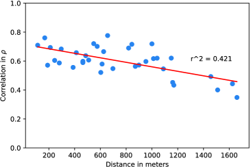
Figure 7: Pairwise correlation between sensors for Oct. 19 and Nov. 10 as functions of their distances.

A3: Pollution concentrations are spatially correlated. We quantify the correlations for further analysis. Figure 7 shows sensor correlations as a function of pairwise distance. The correlation is measured by the Spearman correlation coefficient:

$$\rho=1-\frac{6\sum d_{i}^{2}}{N(N^{2}-1)},$$ (2)

where $d_{i}$ represents the position difference of the paired variables after the two variables are sorted separately and $N$ is the total number of samples. The slope of the fitting line is $0.155\text{\,}{\mathrm{km}}^{-1}$ and the coefficient of determination ($R^{2}$) is 0.421, which implies that closer sensors enable more accurate estimates. Figure 6 shows the sensor correlations during the Nov. 10 and Oct. 19 deployments. We expect the correlations to decrease with increasing inter-sensor distances. The deployment results confirm our hypothesis.

V Experimental Results

In this section, we evaluate the impacts of changing sensor density and using vision-based techniques on estimation accuracy. Specifically, we estimate PM2.5 concentration based on vision-based analysis using transmission information and standard deviation of gray-scale pixel values and compare the performance of several state-of-art estimation algorithms.

V-A Experimental Setup

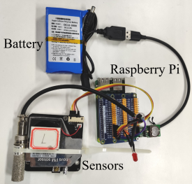
Figure 8: The sensing platform consisting of battery, Raspberry Pi, and sensors.

We design a portable sensing platform to collect, process, and transmit data, as shown in Figure 8. The system battery life is 3.5 hours. The following algorithms are used to estimate pollutant concentration from the measured data.

1. Random forest regression (RFR): This is a widely used algorithm for regression and classification. It combines multiple weak models to form a strong model with much better performance. Random forests contain multiple, unrelated decision trees. The final output depends on the decisions of all trees.

2. Gradient boosting regression (GBR): This method combines a group of weak learners with low complexity and low training cost. It reduces the problem of overfitting and modifies the weights at each training round to produce a strong learner. Gradient boosting modifies its models based on the gradient descent direction of the loss functions of the previously established models.

3. Support vector regression (SVR): Support vector regression aims to find a regression plane with minimal distance to the dataset. Generally, there is a kernel function mapping data to high-dimensional space for better performance on complex manifolds.

The algorithms are implemented using the Python package sklearn. The RFR parameter n_estimators is set to 100 and criterion is set to mean squared error. We set the GBR parameter learning_rate to 0.1 and n_estimators to 100, using least squares regression. We set the SVR parameter c to 1.0 and epsilon to 0.1, using a radial basis function kernel. The parameters are chosen to maximize the training performance. We use the following equation to combine sensor readings and image properties:

$$S(x,t)=G(s_{1}(t),s_{2}(t),...,s_{10}(t),t_{dcp}(t),\beta_{sd}(t)),$$ (3)

where $x$ is the location index, $S(x,t)$ is the concentration estimation at time $t$, $s_{1},s_{2},...,s_{10}$ are the available 10 sensors, $t_{dcp}(t)$ is the transmission information at time $t$, $\beta_{sd}(t)$ is the standard deviation of gray-scale image, and $G$ is the estimation algorithm, which refers to RFR, GBR, or SVR. We use $t_{dcp}(t)$ for low-altitude data and $\beta_{sd}(t)$ for high-altitude data. We later describe how $t_{dcp}(t)$ and $\beta_{sd}(t)$ are obtained for each image in the dataset in section 5.B.

We use data from Jul. 24, Oct. 19, and Nov. 10 for all time stamps and use the mean absolute error (MAE) as the evaluation criteria.

$$\mathit{MAE}=\frac{1}{N}\sum^{N}_{i=1}|y_{i}-\hat{y}_{i}|,$$ (4)

where $y_{i}$ is the actual PM2.5 concentration, and $\hat{y}_{i}$ is the predicted PM2.5 concentration.

There are two classes of images in our dataset. Those in the first class were captured from the ground, on top of a mountain ($78\text{\,}\mathrm{m}$). The second class contains images from a quadcopter flying above the same mountain ($78\text{\,}\mathrm{m}$ + $90\text{\,}\mathrm{m}$). We tried to take the images from the quadcopter and mountain at the same angle and keep the images as similar to each other as possible, but there is some (unavoidable) variation in camera orientation (see Figure 2).

We divide our data into “low-altitude” and “high-altitude” subsets according to the image class and evaluate our algorithms separately on the two classes. We analyze 19 images from the high-altitude dataset and 26 images from the low-altitude dataset. Furthermore, each dataset is divided as follows: 75% of the data and images are randomly selected as a training set and the rest are the testing set. We run the prediction model 50 times per random split of the training and testing datasets.

V-B Image Enhanced Concentration Estimation

Images can be used to estimate PM concentrations in large areas because images can extract the haziness information. We predict PM2.5 concentrations at locations without sensors. Since PM2.5 attenuates light, we estimate PM2.5 concentration in part through the light attenuation coefficient $\beta$ from the haze model. We use the following image features to estimate PM2.5: the dark channel $t_{dcp}(x)$ and the standard deviation $\beta_{sd}$. $t_{dcp}(x)$ is determined using Equation 13 and $\beta_{sd}$ is determined using Equation 21. Figure 9 is an example of applying the dark channel prior to an image. The left image is the original hazy image, and the right image is the transmission estimate for each pixel using dark channel prior. Note that certain kinds of weather conditions like rain and snow might be misinterpreted as pollution. Our PM2.5 estimation algorithm mainly works in sunny and cloudy conditions, which are common in Hangzhou.

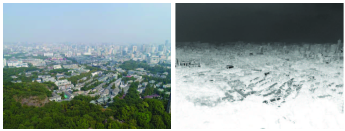
Figure 9: Transmission estimation result.

The atmospheric model describing an image influenced by haze follows [36]:

$$\bm{I}(x)=\bm{J}(x)t(x)+\bm{A}(1-t(x)),$$ (5)

where $x$ is the pixel location, $\bm{I}$ is the observed image, $\bm{J}$ is the scene radiance (image without any haze), $\bm{A}$ is the atmospheric light, $t$ is the transmission function.

Images with higher air pollution tend to look hazier due to lower transmission and contrast. Hence, image features that correlate to haze level enable pollutant concentration estimation.

V-B1 Dark Channel Prior

The dark channel prior, which has been widely used for haze removal, can be used to estimate the transmission of each image pixel. The dark channel prior method is based on the observation that in most haze-free patches, at least one color channel has some pixels with very low intensities. The dark channel is defined as the minimum of all pixel colors in a local patch and can be calculated using the following equation [37]:

$$J_{dark}(x)=\min\limits_{c\in{r,g,b}}\left(\min\limits_{y\in\Omega_{r}(x)}J^{c}(y)\right),$$ (6)

where $J^{c}$ is an RGB channel of $\bm{J}$ and $\Omega_{r}(x)$ is a local patch centered at $x$ with the size of $15\times 15$. Assume the atmospheric light $\bm{A}$ is given and the transmission in a local patch $\Omega_{r}(x)$ is constant, taking the minimum operation in the local patch on Equation 5, we have

$$\min\limits_{y\in\Omega_{r}(x)}\left(I^{c}(y)\right)=\tilde{t}(x)\min\limits_{y\in\Omega_{r}(x)}\left(J^{c}(y)\right)+(1-\tilde{t}(x))A^{c},$$ (7)

where $\tilde{t}(x)$ is the patch’s transmission. The minimum operation is performed on three color channels independently, it is equivalent to

$$\min\limits_{y\in\Omega_{r}(x)}\left(\frac{I^{c}(y)}{A^{c}}\right)=\tilde{t}(x)\min\limits_{y\in\Omega_{r}(x)}\left(\frac{J^{c}(y)}{A^{c}}\right)+(1-\tilde{t}(x)).$$ (8)

By taking the minimum of three color channels, we have

$$\begin{split}\min\limits_{c}\left(\min\limits_{y\in\Omega_{r}(x)}\left(\frac{I^{c}(y)}{A^{c}}\right)\right)=&\tilde{t}(x)\min\limits_{c}\left(\min\limits_{y\in\Omega_{r}(x)}\left(\frac{J^{c}(y)}{A^{c}}\right)\right)\\ &+(1-\tilde{t}(x)).\end{split}$$ (9)

According to the definition of dark channel prior, the dark channel $J_{dark}$ of the haze-free radiance $\bm{J}$ tends to be zero

$$J_{dark}(x)=\min\limits_{c}\left(\min\limits_{y\in\Omega_{r}(x)}J^{c}(y)\right)=0.$$ (10)

Because $A^{c}$ is always positive, this lead to

$$\min\limits_{c}\left(\min\limits_{y\in\Omega_{r}(x)}\frac{J^{c}(y)}{A^{c}}\right)=0.$$ (11)

Substituting Equation 11 into Equation 9, we can estimate the transmission as follows.

$$\tilde{t}(x)=1-\min\limits_{c}\left(\min\limits_{y\in\Omega_{r}(x)}\frac{I^{c}(y)}{A^{c}}\right).$$ (12)

In practice, the atmosphere always contains some haze, which provides depth information. We can optionally keep a small amount of haze by introducing a constant parameter $\omega\ (0<\omega<1)$ into Equation 12

$$\tilde{t}(x)=1-\omega\min\limits_{c}\left(\min\limits_{y\in\Omega_{r}(x)}\frac{I^{c}(y)}{A^{c}}\right).$$ (13)

We fix the value of $\omega$ to 0.95 because this approximates the sparse haze present even on relatively clear days. The atmospheric light $A$ is estimated through this procedure: we pick the top 0.1% brightest pixels in the dark channel and the input image $\bm{I}$ to calculate the atmospheric light. For each hazy image in our dataset, we take the average of the pixel-level transmissions estimated using Equation 13. The resulting average is used for low-altitude data.

V-B2 Standard Deviation

In order to calculate the intensity standard deviation for each image, we convert the RGB image to a gray-scale image, then calculate the standard deviation of all the pixel intensities. The standard deviation is closely related to haze density [38]. The scattering coefficient is a measure of haze density. The higher the scattering coefficient, the higher the haze density. The transmission function is

$$t(x)=e^{\beta d(x)},$$ (14)

where $\beta$ is the scattering coefficient and $d$ is the depth. Substituting Equation 14 into Equation 5, we have

$$\bm{I}_{g}(x)=\bm{J}(x)e^{\beta d(x)}+\bm{A}(1-e^{\beta d(x)}).$$ (15)

The variance of a gray-scale image is

$$\begin{split}\sigma_{I_{g}}^{2}&=\frac{1}{N}\sum_{i=1}^{N}(I_{g}(i)-\frac{1}{N}\sum_{j=1}^{N}I_{g}(j))^{2}\\ &=e^{2\beta d(x)}\frac{1}{N}\sum_{i=1}^{N}(J(i)-\frac{1}{N}\sum_{j=1}^{N}J(j))^{2},\end{split}$$ (16)

where $I_{g}$ is the gray-scale image and $N$ is the number of pixels in the image. When $\beta=0$, we have

$$\sigma_{0}^{2}=\frac{1}{N}\sum_{i=1}^{N}(J(i)-\frac{1}{N}\sum_{j=1}^{N}J(j))^{2}.$$ (17)

Combining Equation 17 and Equation 16 yields

$$\sigma_{I_{g}}=e^{-2\beta}\sigma_{0}^{2}.$$ (18)

After taking the logarithm of both sides, the scattering coefficient can be expressed as

$$\beta=\rm{ln}\ \sigma_{0}-\rm{ln}\ \sigma_{I_{g}}.$$ (19)

Since $\sigma$ is changed at each image, Equation 19 can be expressed using the first-order Taylor Series approximation

$$\beta=1+\rm{ln}\ \sigma_{0}-\sigma_{I_{g}}.$$ (20)

When $\beta=0$, the variance of the scene radiance approximates 1. Thus we have

$$\beta=1-\rm{ln}\ \sigma_{I_{g}}.$$ (21)

Therefore we can estimate the concentration using the standard deviation of the gray-scale image. The standard deviation is used for high-altitude data.

V-C Concentration Estimation Results

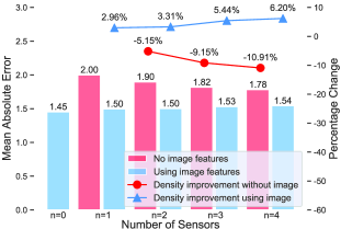
Figure 10: The relationship between mean average error and sensor density for Gradient Boosting Regression on high-altitude data.

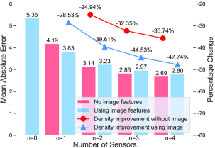
Figure 11: The relationship between mean average error and sensor density for Gradient Boosting Regression on low-altitude data.

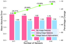
Figure 12: The relationship between mean average error and using images for Gradient Boosting Regression on high-altitude data.

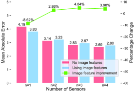
Figure 13: The relationship between mean average error and using images for Gradient Boosting Regression on low-altitude data.

For each available sensor deployment location, we speculatively remove one or more sensor’s data and use estimation techniques with access to the remaining sensors to infer concentration(s), thereby allowing comparison with ground truth measurements. We investigate the impact of the number of sensors on the estimation accuracy by using all possible combinations of speculatively removed sensors and averaging the results. We also consider the impact of using image data on estimation accuracy.

We plotted the results from the best-performing algorithm: GBR. The density improvements in Figures 10 and 11 are compared with the $n=0$ (no images) case. If image features are used, the improvements are compared with the $n=1$ case. Note that the lower MAE is, the better the estimation accuracy. Thus a negative change indicates improvement. The bars in Figures 10–13 represent the MAE resulting from using different numbers of sensors. The lower bars indicate higher accuracies. The lines in Figures 10–13 indicate percentage change to MAE in different cases (e.g., using images or more sensors). The lower the percentage change, the larger the improvement, and positive percentage changes imply (undesirable) increases in MAE.

As sensor density increases, the estimation MAE decreases. This implies that accuracy improves with sensor density, even at densities much higher than those of modern stationary sensor deployments. Moreover, as shown in Figure 7, sensor correlations decrease with increasing distance. This is the reason estimation accuracy improves with increasing sensor density. Using the four nearest sensors instead of one sensor improves estimation accuracy by 23.3% on average without using images, and 20.75% when using images. The fact that increasing sensor density improves accuracy less when images are available does not imply that images are unhelpful. In contrast, it implies that using images allows higher accuracy when few sensors are available, leaving less potential for improvement if sensor density is later increased.

A4 Vision-based techniques significantly improve estimation accuracy. As shown in Figures 12 and 13, PM2.5 concentration prediction accuracy improves when images are used. In the case of $n=0$, we average all the available concentrations. The MAE is $20.821\text{\,}\mathrm{\SIUnitSymbolMicro g}\text{\,}{\mathrm{m}}^{-3}$ for high-altitude data and $6.929\text{\,}\mathrm{\SIUnitSymbolMicro g}\text{\,}{\mathrm{m}}^{-3}$ for low-altitude data. The high-altitude images enable higher accuracy because some sensor locations are occluded in the low-altitude images. When images are used, MAE drops to $1.45\text{\,}\mathrm{\SIUnitSymbolMicro g}\text{\,}{\mathrm{m}}^{-3}$ and $5.35\text{\,}\mathrm{\SIUnitSymbolMicro g}\text{\,}{\mathrm{m}}^{-3}$ respectively. For the case where $n=1$, when we use the PM2.5 concentrations of the nearest available sensor for estimation image data improves prediction accuracy by 16.9% on average. The benefits of using images are greatest when the fewest particle counters are used.

To determine whether the improvement is systemic and statistically significant, we use the Kolmogorov-Smirnov test. We compare the data for the MAE without using images that using images for each number of sensors ($n=1,...,4$) to determine whether the two data sets have the same distribution. The test is non-parametric and requires no knowledge about the distribution of data.

We determine that there is a statistically significant difference between the distribution of the MAE when using images and the distribution without using images, i.e., the difference between the two distributions is not due only to chance or noise but due to a genuine improvement in accuracy when using the image data. If the p-value is below 0.10, we can reject the null hypothesis and conclude that using images does improve our results. As shown in Table VIII and Table IX, on low-altitude data, the p-values of GBR in all cases are less than 0.10, and on high-altitude data, GBR’s p-values are less than 0.10. As a result, we are confident that using images improves the estimates.

TABLE VIII: P-Values of GBR on High-Altitude Data.

GBR
n=1	n=2	n=3	n=4
$<0.001$	$<0.001$	$<0.001$	$0.064$

TABLE IX: P-Values of GBR on Low-Altitude Data.

GBR
n=1	n=2	n=3	n=4
$0.068$	$<0.001$	$<0.001$	$<0.001$

Certain fixed-location images show slightly negative results for the GBR method. Since the fixed-location images are taken from a low altitude, some of the sensor locations are blocked by buildings. For the quadcopter images taken at a higher altitude, all estimation techniques improve accuracy. In general, images decrease MAE by 8.44% on average, when $n\leqslant 1$, adding a camera to collect images helps more than adding more sensors.

Increasing sensor density and using images change the relative accuracy of the estimation algorithms. When we use only one sensor and no images, RFR has lower MAE than GBR on low-altitude data. When the sensor density is increased ($n=4$) and images are used, GBR outperforms RFR. This result demonstrates that it is important to evaluate estimation algorithms using appropriate sensor densities and access to image data. A sparsely deployed and less accurate sensor network can lead to false conclusions about pollution concentrations, and about which pollution concentration estimation algorithms are most accurate.

To summarize, higher sensor densities and image data both improve estimation accuracy, and adding image data has a similar effect to increasing particle counter density by 0.61 sensors $\text{\,}{\mathrm{km}}^{-2}$. Of the three estimation techniques evaluated, GBR had the highest accuracy with MAE=$1.45\text{\,}\mathrm{\SIUnitSymbolMicro g}\text{\,}{\mathrm{m}}^{-3}$. In particular, our developed method is unlikely to work as well on night-time images and images with adverse weather conditions such as rain and snow. The main limitation of our dataset is that it does not contain nighttime images.

VI Conclusion

This paper presents a PM dataset with high spatial and temporal resolution. In contrast with existing datasets, HVAQ contains images covering the locations of stationary point sensors, making it suitable for evaluating and validating vision-based pollution estimation algorithms. Through our analysis, we find that (1) the estimation accuracy can be improved significantly using vision-based techniques; (2) the spatial pollutant distribution is spatially correlated; (3) spatial variation of PM2.5 is high; and (4) temperature and humidity had limited impact on PM concentration in our dataset. We also evaluate our data using state-of-art prediction methods. Accuracy correlates with density with a coefficient of $0.2875\text{\,}\mathrm{\SIUnitSymbolMicro g}\text{\,}{\mathrm{m}}^{-3}$ MAE per sensor and vision-based estimation improves accuracy by $0.1813\text{\,}\mathrm{\SIUnitSymbolMicro g}\text{\,}{\mathrm{m}}^{-3}$ MAE, on average.

References

- [1] K. Naddafi, M. S. Hassanvand, M. Yunesian, F. Momeniha, R. Nabizadeh, S. Faridi, and A. Gholampour, “Health impact assessment of air pollution in megacity of Tehran, Iran,” Iranian J. of Environmental Health Science & Engineering, vol. 9, no. 1, p. 28, 2012.
- [2] H. Nourmoradi, Y. O. Khaniabadi, G. Goudarzi, S. M. Daryanoosh, M. Khoshgoftar, F. Omidi, and H. Armin, “Air quality and health risks associated with exposure to particulate matter: a cross-sectional study in Khorramabad, Iran,” Health Scope, vol. 5, no. 2, 2016.
- [3] S. Poduri, A. Nimkar, and G. S. Sukhatme, “Visibility monitoring using mobile phones,” Annual Report: Center for Embedded Networked Sensing, pp. 125–127, 2010.
- [4] B. Chen and H. Kan, “Air pollution and population health: a global challenge,” Environmental Health and Preventive Medicine, vol. 13, no. 2, pp. 94–101, 2008.
- [5] F. J. Kelly and J. C. Fussell, “Air pollution and public health: emerging hazards and improved understanding of risk,” Environmental Geochemistry and Health, vol. 37, no. 4, pp. 631–649, 2015.
- [6] S. Feng, D. Gao, F. Liao, F. Zhou, and X. Wang, “The health effects of ambient PM2. 5 and potential mechanisms,” Ecotoxicology and Environmental Safety, vol. 128, pp. 67–74, 2016.
- [7] J. O. Anderson, J. G. Thundiyil, and A. Stolbach, “Clearing the air: a review of the effects of particulate matter air pollution on human health,” J. of Medical Toxicology, vol. 8, no. 2, pp. 166–175, 2012.
- [8] R. A. Rohde and R. A. Muller, “Air pollution in China: mapping of concentrations and sources,” PloS one, vol. 10, no. 8, 2015.
- [9] Y. Zhang, J. Cai, S. Wang, K. He, and M. Zheng, “Review of receptor-based source apportionment research of fine particulate matter and its challenges in China,” Science of the Total Environment, vol. 586, pp. 917–929, 2017.
- [10] G. Lin, J. Fu, D. Jiang, W. Hu, D. Dong, Y. Huang, and M. Zhao, “Spatio-temporal variation of PM2. 5 concentrations and their relationship with geographic and socioeconomic factors in China,” Int. J. of Environmental Research and Public Health, vol. 11, no. 1, pp. 173–186, 2014.
- [11] X. Zhao, W. Zhou, L. Han, and D. Locke, “Spatiotemporal variation in PM2. 5 concentrations and their relationship with socioeconomic factors in China’s major cities,” Environment Int., vol. 133, p. 105145, 2019.
- [12] C. Zhang, J. Yan, C. Li, X. Rui, L. Liu, and R. Bie, “On estimating air pollution from photos using convolutional neural network,” in Proc. Int. Conf. on Multimedia, pp. 297–301, 2016.
- [13] T. Zhang and R. P. Dick, “Estimation of multiple atmospheric pollutants through image analysis,” in Proc. Int. Conf. on Image Processing, pp. 2060–2064, 2019.
- [14] Y. Li, J. Huang, and J. Luo, “Using user generated online photos to estimate and monitor air pollution in major cities,” in Proc. Int. Conf. on Internet Multimedia Computing and Service, pp. 1–5, 2015.
- [15] C. Liu, F. Tsow, Y. Zou, and N. Tao, “Particle pollution estimation based on image analysis,” PloS one, vol. 11, no. 2, p. e0145955, 2016.
- [16] J. S. Apte, K. P. Messier, S. Gani, M. Brauer, T. W. Kirchstetter, M. M. Lunden, J. D. Marshall, C. J. Portier, R. C. Vermeulen, and S. P. Hamburg, “High-resolution air pollution mapping with Google street view cars: exploiting big data,” Environmental Science & Technology, vol. 51, no. 12, pp. 6999–7008, 2017.
- [17] Y. Guan, M. C. Johnson, M. Katzfuss, E. Mannshardt, K. P. Messier, B. J. Reich, and J. J. Song, “Fine-scale spatiotemporal air pollution analysis using mobile monitors on Google street view vehicles,” J. of the American Statistical Association, vol. 115, no. 531, pp. 1111–1124, 2020.
- [18] J. Wei, Z. Li, W. Xue, L. Sun, T. Fan, L. Liu, T. Su, and M. Cribb, “The ChinaHighPM10 dataset: generation, validation, and spatiotemporal variations from 2015 to 2019 across China,” Environment Int., vol. 146, p. 106290, 2021.
- [19] J. Khan, K. Kakosimos, O. Raaschou-Nielsen, J. Brandt, S. S. Jensen, T. Ellermann, and M. Ketzel, “Development and performance evaluation of new AirGIS–a GIS based air pollution and human exposure modelling system,” Atmospheric environment, vol. 198, pp. 102–121, 2019.
- [20] C. Wen, S. Liu, X. Yao, L. Peng, X. Li, Y. Hu, and T. Chi, “A novel spatiotemporal convolutional long short-term neural network for air pollution prediction,” Science of the Total Environment, vol. 654, pp. 1091–1099, 2019.
- [21] G. Janssens-Maenhout, F. Dentener, J. Van Aardenne, S. Monni, V. Pagliari, L. Orlandini, Z. Klimont, J.-i. Kurokawa, H. Akimoto, T. Ohara et al., “EDGAR-HTAP: a harmonized gridded air pollution emission dataset based on national inventories,” European Commission Publications Office, Ispra (Italy). JRC68434, EUR report, vol. 25, pp. 299–2012, 2012.
- [22] S. De Vito, E. Massera, M. Piga, L. Martinotto, and G. Di Francia, “On field calibration of an electronic nose for benzene estimation in an urban pollution monitoring scenario,” Sensors and Actuators B: Chemical, vol. 129, no. 2, pp. 750–757, 2008.
- [23] J. J. Li, B. Faltings, O. Saukh, D. Hasenfratz, and J. Beutel, “Sensing the air we breathe: the OpenSense Zurich dataset,” in AAAI Conf. on Artificial Intelligence, 2012.
- [24] Y. Yang, Z. Hu, K. Bian, and L. Song, “Imgsensingnet: Uav vision guided aerial-ground air quality sensing system,” in IEEE INFOCOM 2019-IEEE Conf. on Computer Communications, pp. 1207–1215. IEEE, 2019.
- [25] P. G. Herzog and B. Hill, “Multispectral imaging and its applications in the textile industry and related fields,” in PICS, pp. 258–263, 2003.
- [26] F. Martínez-Verdú, J. Pujol, and P. Capilla, “Characterization of a digital camera as an absolute tristimulus colorimeter,” J. of Imaging Science and Technology, vol. 47, no. 4, pp. 279–295, 2003.
- [27] A. M. Nahavandi, “Metric for evaluation of filter efficiency in spectral cameras,” Applied optics, vol. 55, no. 32, pp. 9193–9204, 2016.
- [28] N. Rijal, R. T. Gutta, T. Cao, J. Lin, Q. Bo, and J. Zhang, “Ensemble of deep neural networks for estimating particulate matter from images,” in 2018 IEEE 3rd Int. Conf. on image, Vision and Computing, pp. 733–738. IEEE, 2018.
- [29] K. Gu, J. Qiao, and X. Li, “Highly efficient picture-based prediction of PM2. 5 concentration,” IEEE Trans. on Industrial Electronics, vol. 66, no. 4, pp. 3176–3184, 2018.
- [30] H. Grimm and D. J. Eatough, “Aerosol measurement: the use of optical light scattering for the determination of particulate size distribution, and particulate mass, including the semi-volatile fraction,” J. of the Air & Waste Management Association, vol. 59, no. 1, pp. 101–107, 2009.
- [31] M. Kamionka, P. Breuil, and C. Pijolat, “Calibration of a multivariate gas sensing device for atmospheric pollution measurement,” Sensors and Actuators B: Chemical, vol. 118, no. 1-2, pp. 323–327, 2006.
- [32] G. Liu, J. Li, D. Wu, and H. Xu, “Chemical composition and source apportionment of the ambient PM2. 5 in Hangzhou, China,” Particuology, vol. 18, pp. 135–143, 2015.
- [33] Q. Jin, R. Ren, and L. Gong, “Research on the elemental characterization and source apportionment of PM2.5 in main urban area of Hangzhou,” Chinese J. of Health Laboratory Technology, vol. 27, no. 22, pp. 3200–3205, 2017.
- [34] J. Wu, C. Xu, Q. Wang, and W. Cheng, “Potential sources and formations of the PM2.5 pollution in urban Hangzhou,” Atmosphere, vol. 7, no. 8, p. 100, 2016.
- [35] Q. Zhu, Y. Liu, W. Xu, and M. Huang, “Analysis on the pollution characteristics and influence factors of pm2. 5 in guangzhou,” Environ. Monit. China, vol. 29, no. 2, p. 15, 2013.
- [36] S. G. Narasimhan and S. K. Nayar, “Vision and the atmosphere,” Int. J. of Computer Vision, vol. 48, no. 3, pp. 233–254, 2002.
- [37] K. He, J. Sun, and X. Tang, “Single image haze removal using dark channel prior,” IEEE Trans. on Pattern Analysis and Machine Intelligence, vol. 33, no. 12, pp. 2341–2353, 2010.
- [38] D. Park, D. K. Han, C. Jeon, and H. Ko, “Fast single image de-hazing using characteristics of RGB channel of foggy image,” IEICE Trans. on Information and Systems, vol. 96, no. 8, pp. 1793–1799, 2013.