The nonlocal dielectric response of water in nanoconfinement

Abstract

Recent experiments reporting a very low dielectric permittivity for nanoconfined water have renewed the interest to the structure and dielectric properties of water in narrow gaps. Here, we describe such systems with a minimal Landau-Ginzburg field-theory composed of a nonlocal bulk-determined term and a local water-surface interaction term. We show how the interplay between the boundary conditions and intrinsic bulk correlations encodes dielectric properties of confined water. Our theoretical analysis is supported by molecular dynamics simulations and comparison with the experimental data.

Introduction - Interest in the dielectric properties of confined water has been boosted by the remarked measurement of the dielectric permittivity of nanometric water layer confined between hydrophobic surfaces [1]. Fumagali et al. reported an anomalously low dielectric constant in the direction perpendicular to the surface. [2] Water permittivity in the vicinity of a surface is inhomogeneous[3, 4] leading to a significant increase of the electrostatic interactions, as postulated in the 1950’s by Schellman,[5] and observed experimentally and in simulations [6, 7, 8]. The stability of emulsions and colloidal solutions [9, 10], ion transport and reactivity in channels of proteins,[11], in subsystems of geological interest [12] or in nanotechnologic devices [13] are strongly influenced by electrostatic properties of confined water. However, a fundamental analytic theory connecting the dielectric response to the properties of the confining surfaces, namely chemical composition, degree and geometry of confinement, is still outstanding.[14] At the molecular scale, the relative dielectric permittivity tensor $\epsilon_{\alpha,\beta}(\vec{r}-\vec{r^{\prime}})$ of bulk water is non local.[15, 16, 17] The structuration in the fluid at an interface induced by this nonlocality has been widely studied at the atomic scale using molecular dynamics (MD) simulations [18, 19, 20, 21, 22]. At a coarse-grained scale, continuum nonlocal electrostatics provide a useful framework to quantify the dielectric properties of confined correlated fluids. [19] This can be based on phenomenological energy functionals that are written in terms of the polarization field ${\vec{m}}$. They are the sum of the electrostatic energy depending on the displacement field ${\vec{D}_{0}}$ and of a correlation term [23, 24, 25, 26]. It reads

$$\mathcal{U}_{\mathrm{bulk}}[\vec{m},\vec{D}_{0}]=\frac{1}{2\epsilon_{0}}\int{d\vec{r}\left(\vec{D}_{0}-\vec{m}(\vec{r})\right)^{2}}\\ +\frac{1}{2\epsilon_{0}}\int{d\vec{r}d\vec{r^{\prime}}m^{\alpha}(\vec{r})\mathcal{K}_{\alpha,\beta}(\vec{r},\vec{r^{\prime}})m^{\beta}(\vec{r^{\prime}})},$$ (1)

where $\epsilon_{0}$ is the vacuum dielectric permittivity.

We specify the kernel $\mathcal{K}_{\alpha,\beta}(\vec{r},\vec{r^{\prime}})$ to mimic the simulated nonlocal dielectric properties of bulk water. We further introduce a phenomenological interaction energy between the surface and the fluid as a sum of harmonic potentials. We show that this framework reproduces both MD simulations for two hydrophobic surfaces, graphene and hexagonal boron nitride (hBN), and an experimental data.[1] In addition, it formalizes the effect of the confining material on the dielectric properties of ’interfacial water’.

Bulk water - The dielectric properties of bulk water are encoded in the two-points susceptibility tensor $\chi_{\alpha,\beta}(\vec{r}-\vec{r^{\prime}})=\delta_{\alpha,\beta}(\vec{r}-\vec{r^{\prime}})-\epsilon^{-1}_{\alpha,\beta}(\vec{r}-\vec{r^{\prime}})$. This nonlocal kernel can be expressed through the correlations of the polarization ${\vec{m}}$ using the classical approximation for the fluctuation-dissipation theorem,

$$\chi_{\alpha,\beta}(\vec{r}-\vec{r^{\prime}})=\frac{\langle m_{\alpha}(\vec{r})m_{\beta}(\vec{r^{\prime}})\rangle}{\epsilon_{0}k_{B}T}.$$ (2)

The correlations $\langle m_{\alpha}(\vec{r})m_{\beta}(\vec{r^{\prime}})\rangle$ can be written in terms of the experimentally measured partial HH, OH, OO structure factors of water[28] under the assumption of simple point charges localized at the atoms of molecules.[17] The $q-$dependence of longitudinal part of the susceptibility in the Fourier space $\hat{\chi}_{\parallel}(q)$ illustrates the nonlocal nature of dielectric properties water (see Fig. 1). The main peak of $\hat{\chi}_{\parallel}(q)$ (centered at $q=$30\text{\,}\mathrm{n}\mathrm{m}^{-}\mathrm{1}$$) exceeds 1, corresponding to a range of wavelengths associated with a negative permittivity $\epsilon_{\parallel}(q)=1/(1-\chi_{\parallel}(q))$. This overscreening zone is a consequence of the H-bonding network in water[17].

To model these properties, we follow a Landau-Ginzburg (LG) approach which proved its value in the study of critical surface phenomena.[29] We choose the following form of the second item in Eq.(1),

$$\mathcal{U}_{m}[\vec{m}]=\int{\frac{d\vec{r}}{2\epsilon_{0}}\left(K\vec{m}^{2}+K_{l}\left(\vec{\nabla}\vec{m}\right)^{2}+\beta\left(\vec{\nabla}\left(\vec{\nabla}\vec{m}\right)\right)^{2}\right)},$$ (3)

which includes terms up to second spacial derivative of the field and leads to the longitudinal susceptibility,

$$\hat{\chi}_{\parallel}(q)=\frac{1}{1+K+K_{l}q^{2}+\beta q^{4}}.$$ (4)

For derivation and discussion see the supporting material (SM). The model parameters ($K$, $K_{l}$ and $\beta$) are chosen to capture: (i) the permittivity of bulk water at $q=0$, (ii) the position of the first peak and (iii) its width at half height of the simulated or experimentally recovered $\chi_{\parallel}(q)$. The theoretical susceptibility is plotted in red in Fig. 1.

Its poles define a decay length $\lambda_{d}$ and a period $\lambda_{o}$,

$$\lambda_{d}=\frac{2\sqrt{\beta}}{\sqrt{2\sqrt{(\beta(1+K)}+K_{l}}},\>\lambda_{o}=\frac{4\pi\sqrt{\beta}}{\sqrt{2\sqrt{\beta(1+K)}-K_{l}}},$$ (5)

characterizing the polarization correlations in bulk. They are equal to $\lambda_{d}=$2.1\text{\,}\mathrm{\SIUnitSymbolAngstrom}$$ and $\lambda_{o}=$2.1\text{\,}\mathrm{\SIUnitSymbolAngstrom}$$ for the chosen parametrization.

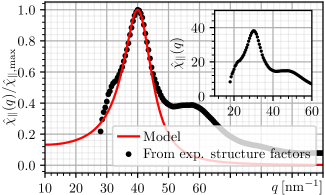
Figure 1: Dielectric susceptibility of bulk water. Black dots are recovered from inelastic neutron scattering data for oxygen-oxygen, hydrogen-hydrogen, and oxygen-hydrogen structure factors.[17, 28] Red curve has been computed from Eq. (4) with $K=1/70$, $K_{l}=$-2.01\text{\times}{10}^{-3}\text{\,}\mathrm{n}\mathrm{m}^{-2}$$, $\beta=$1.12\text{\times}{10}^{-6}\text{\,}\mathrm{n}\mathrm{m}^{-4}$$. The inset shows the susceptibility which has not been normalized to 1.

Theoretical model for interfacial water - We consider water delimited by a planar interface infinite in the $xy$ plane and located at $z$=0 (See Fig. 2a). A static homogeneous external field $\vec{D}_{0}=D_{0}\vec{u}_{z}$ is applied in the z-direction. According to the symmetry of the problem, this field excites exclusively the longitudinal polarization that depends on $z$: $\vec{m}(\vec{r})=m(z)\vec{u}_{z}$. We write the energy of the system per unit area $U[m,D_{0}]=U_{\mathrm{bulk}}+U_{s}$, the sum of the bulk-determined term, $U_{\mathrm{bulk}}$, derived from (Eqs. 1,3), and a surface term $U_{s}$ as

$$U_{\mathrm{bulk}} = \int^{\infty}_{z=0}{\frac{dz}{2\epsilon_{0}}\left[\left(D_{0}-m\right)^{2}+Km^{2}+K_{l}\dot{m}^{2}+\beta\ddot{m}^{2}\right]}$$

$$U_{s} = \frac{k_{m}}{2}\left(m(0)-m_{0})\right)^{2}+\frac{k_{\rho}}{2}\left(\rho(0)-\rho_{0})\right)^{2}$$ (6)

where the upper dot stands for the spatial derivation along $z$. In the spirit of the LG development used to express the kernel $\mathcal{K}$ (Eq. (1)), $U_{s}$ is written as an expansion of elastic energies[29, 30] depending on the polarization field and its derivative $\dot{m}(z)$, equal to minus the bound charge, $\rho(z)$.[31] The major contribution promotes a surface polarization $m_{0}$ and the corrective second term favors a water charge density $\rho_{0}$ at the interface. The stiffnesses $k_{m}$ and $k_{\rho}$ quantify the strength of the boundary conditions. In the strong interaction limit $(k_{m},k_{\rho})\rightarrow\infty$, the surface fixes both polarization and charge density at interface.

The partition function of the system, $\mathcal{Z}[D_{0}]=\int{D[m_{z}]\exp{\left[-\left(U_{\mathrm{bulk}}[m,D_{0}]+U_{s}\right)/k_{B}T\right]}},$ can be split in the form

$$\mathcal{Z}[D_{0}]=\int d\bar{m}d\bar{\rho}\exp{\left[\frac{1}{k_{B}T}\left(\frac{k_{m}}{2}(\bar{m}-m_{0})^{2}+\frac{k_{\rho}}{2}(\bar{\rho}-\rho_{0})^{2}\right)\right]}\int^{\begin{subarray}{c}m(z\rightarrow\infty)=0\\ \dot{m}(z\rightarrow\infty)=0\end{subarray}}_{\begin{subarray}{c}m(0)=\bar{m}\\ \dot{m}(0)=-\bar{\rho}\end{subarray}}{D[m]\exp{\left[-\frac{1}{k_{B}T}U_{\mathrm{bulk}}[m,D_{0}]\right]}}.$$ (7)

This includes a partition of the fields $m(z)$ satisfying the boundary conditions (right integral), then a sampling of the $z=0$ boundary conditions $(\bar{m},\bar{\rho})$ (left integral). We find the mean field solution, $m_{1}(z)$, by first minimizing $U_{\mathrm{bulk}}[m,D_{0}]$ with respect to $m(z)$ leading to

$$(1+K)m(z)-K_{l}m^{(2)}(z)+\beta m^{(4)}(z)=D_{0},$$ (8)

with $m(0)=\bar{m}$, $\dot{m}(0)=-\bar{\rho}$, $m(z\rightarrow\infty)=0$, $\dot{m}(z\rightarrow\infty)=0$. The solution of which is

$$m_{1}(z)=\frac{D_{0}}{1+K}\left(1-e^{-\frac{z}{\lambda_{d}}}\left(\cos(q_{o}z)+\frac{q_{d}}{q_{o}}\sin(q_{o}z)\right)\right)$$ (9)

$$+ e^{-\frac{z}{\lambda_{d}}}\left(\bar{m}\left(\cos(q_{o}z)+\frac{q_{d}}{q_{o}}\sin(q_{o}z)\right)-\frac{\bar{\rho}}{q_{0}}\sin(q_{o}z)\right).$$

with $q_{o}=2\pi/\lambda_{o}$ and $q_{d}=1/\lambda_{d}$, the wavenumbers of the bulk correlations. Second, we extremalize the total energy of the system, $U=U_{\mathrm{bulk}}+U_{s}$, with respect to $(\bar{m},\bar{\rho})$ obtained by injecting $m_{1}(z)$ in Eqs. (The nonlocal dielectric response of water in nanoconfinement) and performing the integral over $z$ (see SM). The nature of the extremum depends on the dimensionless stiffness constants $(\tilde{k}_{m},\tilde{k}_{\rho})$, given in the SM. $U(\bar{m},\bar{\rho})$ admits a minimum for $\tilde{k}_{m}$ and $\tilde{k}_{\rho}$ belonging to the pointed zone represented in Fig. 2b, to which we restrict our study in the following. The mean field polarization $m_{2}(z)$ is given by Eq. (9) for $\bar{m}=m_{s},\bar{\rho}=\rho_{s}$, the boundary conditions minimizing $U(\bar{m},\bar{\rho})$. Their expressions are given in SM.

To study the dielectric properties of interfacial water, we introduce the real space susceptibility, $\chi(z)=dm_{2}(z)/dD_{0}$ derived from Eq. (9). It quantifies the response to a homogeneous external field $D_{0}$ and is constant and equal to $\chi_{b}=\hat{\chi}(0)$ for bulk water.

Fig. 2c, d show typical mean field polarization $m_{2}(z)$ and susceptibility $\chi(z)$ in the interfacial water. We observe a nonvanishing polarization and a nonconstant $\chi(z)$ that are oscillating functions of period $\lambda_{o}$ in an exponentially decaying envelope of range $\lambda_{d}$. The surface induces a layering of the fluid that extends over about $1\text{\,}\mathrm{n}\mathrm{m}$, a lengthscale consistent with many previous simulations of interfacial water[3, 32]. The susceptibility shows alternation of underresponding ($\chi(z)\ll\chi_{b}$) and overresponding layers ($\chi(z)\gg\chi_{b}$), typical for overscreening effect. Whereas the amplitude of $m_{2}(z)$ is a non-trivial function of the bulk properties, the four parameters of the surface interaction and $D_{0}$, the amplitude of $\chi(z)$ does not depend on ($m_{0},\rho_{0},D_{0}$). The interface affects the dielectric properties of water only through the stiffnesses $(\tilde{k}_{m},\tilde{k}_{\rho})$.

We first study the case of vanishing $\tilde{k}_{\rho}$ for which $\chi(z)_{\tilde{k}_{\rho}=0}$ can be written as

$$\frac{\chi(z)_{\tilde{k}_{\rho}=0}}{\chi_{b}}=1+\frac{\tilde{k}_{m}e^{-q_{d}z}}{1-\tilde{k}_{m}}\left(\cos(q_{o}z)+\frac{q_{d}^{2}-q_{o}^{2}}{2q_{d}q_{o}}\sin(q_{o}z)\right).$$ (10)

The amplitude of $\chi(z)_{\tilde{k}_{\rho}=0}$ decreases with $\tilde{k}_{m}$ and tends to a finite value for $\tilde{k}_{m}\gg 1$. This case is represented in Fig. 2e (blue curve). Then we consider the corrective effect of $\tilde{k}_{\rho}$ in the limit of a large $\tilde{k}_{m}$ by studying

$$\frac{\chi(z)_{\tilde{k}_{m}\gg 1}}{\chi_{b}}=\frac{\chi(z)_{\tilde{k}_{m}\gg 1,\tilde{k}_{\rho}=0}}{\chi_{b}}-\frac{q_{d}^{2}+q_{o}^{2}}{2q_{d}q_{o}}\frac{\tilde{k}_{\rho}e^{-q_{d}z}}{1+\tilde{k}_{\rho}}\sin(q_{o}z).$$ (11)

An increasing $\tilde{k}_{\rho}$ induces a dephasing and an amplitude decrease up to a factor 2 of $\chi(z)$ (See  2e). The behavior of $\chi(z)$ as a function of $(\tilde{k}_{m},\tilde{k}_{\rho})$ illustrates that different surfaces, having stronger or weaker influence on polarization and partial charge, induce different dielectric properties of interfacial water.

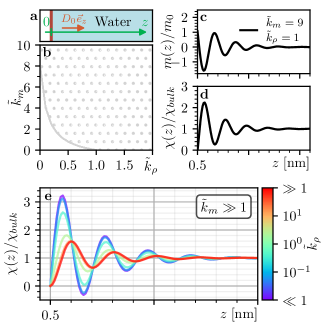
Figure 2: Dielectric properties of water in the vicinity of a surface. a. Sketch of the system. b. Diagram presenting the zone of finite minimum (dotted zone) as a function of $\tilde{k}_{m}$ and $\tilde{k}_{\rho}$. Profile of the polarization $m(z)$ (c) and the normalized susceptibility $\chi(z)$ (d) computed for ($\tilde{k}_{m}=9,\tilde{k}_{\rho}=1$) and ($m_{0}=$-10\text{\,}\mathrm{V}\mathrm{/}\mathrm{n}\mathrm{m}$,\rho_{0}/q_{o}=$-10\text{\,}\mathrm{V}\mathrm{/}\mathrm{n}\mathrm{m}$$). e. Susceptibility normalized to the bulk susceptibility computed from Eq. (11) with different values of $\tilde{k}_{\rho}$.

Comparison with MD simulations - We performed MD simulations of pure water confined in a slab geometry using the GROMACS MD simulation package.[34] Water molecules are described with the SPC/E model and the walls are made up of atoms of frozen positions. We considered graphene and hBN surfaces ( details in the SM).

We analyze the polarization, $m_{\rm{MD}}(z)=-\int^{z}_{0}dz\rho_{\rm{MD}}(z)dz$, with $\rho_{\rm{MD}}$ the charge density of water, and the susceptibility $\chi_{\rm{MD}}(z)=(m_{\rm{MD}}(z,D_{0}+\delta D_{0})-m_{{\rm{MD}}}(z,D_{0}))/\delta D_{0}$ [3] with $\delta D_{0}=0.5V/nm$, in the vicinity of the surfaces. The profiles are similar for both surfaces (Fig. 3): first, a vacuum layer ($m_{\rm{MD}}(z)=0$, $\chi_{\rm{MD}}(z)=0$) between the surface and the liquid, due to the repulsive part of the surface-fluid Lennard-Jones (LJ) interaction, then decaying oscillations over about $1\text{\,}\mathrm{n}\mathrm{m}$ before reaching the bulk value. The theoretical decay $\lambda_{d}$ and the period $\lambda_{o}$ are in very good agreement with the simulated ones (see SM). This validates the derivation of the characteristic lengths of interfacial water from the bulk dielectric susceptibility, $\hat{\chi}(q)$.

In MD simulations, the position of the interfaces is not as clear-cut as in theory due to thermal capillary fluctuations and the non-infinitly sharp repulsion of the surface-fluid LJ interaction.[35] This is taken into account by applying a smearing to the theoretical predictions,

$$\tilde{f}(z)=\left(G\ast(\theta f)\right)(z+z_{0}),\>G(z)=\frac{e^{-z^{2}/2\eta^{2}}}{\eta\sqrt{2\pi}},$$ (12)

with $\theta$ being the Heaviside function and $f$ standing for $m$ or $\chi$. The position $z_{0}$ and the standard deviation $\eta$ are determined for each surface by fitting the first oxygen density peak with a Gaussian $G(z)$ which position and width define $z_{0}$ and $\eta$ (see SM for details). The hBN surface is characterized by a deeper LJ potential and consequently a smaller dispersion $\eta$ than the graphene. Correspondly, $m_{\rm MD}(z)$ amplitude is smaller in interfacial water for graphene than for hBN Figs. 3a-b.

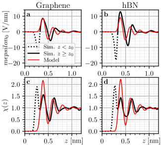
Figure 3: Comparison between model (in red) and MD simulations (in black) for a graphene layer (left panels) and a hBN layer (right panels). Top (respectively bottom) panels show the polarization (respectively the susceptibility). Simulation curves for $z\leq z_{0}$ are represented with dotted lines.

We validate the theoretical model in three steps. First, we adjust the simulated susceptibilities with $\tilde{\chi}(z)$ defined in Eq. (12). If we choose ($\tilde{k}_{m}\gg 1$, $\tilde{k}_{\rho}=0$) for graphene and ($\tilde{k}_{m}\gg 1$, $\tilde{k}_{\rho}=0.2$) for hBN, we obtain a good agreement between the calculated and the simulated value of the susceptibilities as shown in figures 3c-d. Next, we fit the simulated polarization for graphene surface with $\tilde{m}(z)$ by fixing $m_{0}$, the single left unknown parameter for graphene as $\tilde{k}_{\rho}=0$. Finally, we fit the simulated polarization for a hBN surface. Taking the surface polarization $m_{0}$ previously determined in the case of graphene, we fix $\rho_{0}$. The comparison between theoretical and simulated polarization are presented in Figs. 3a-b. The dotted part of the simulated curves correspond to the vacuum gap and the contribution of hydrogen located in $z<z_{0}$. The theoretical model describes this zone as a vacuum gap (see Eq. (12)).

Graphene and hBN surfaces are parametrized by $\tilde{k}_{m}\gg 1$, thus both surfaces freeze the interfacial polarization to $m(z_{0})=m_{0}$ which does respond to $D_{0}$. At the microscopic scale, this result can be interpreted as the effect of the vacuum gap on the organization in the first layer of water which optimizes the number of H-bonds.[36] Most likely, $\tilde{k}_{m}$ is very large for a wide variety of surfaces, both hydrophobic and hydrophilic, as they impose a layout in the first hydration layer.[3, 37] For a non-vanishing corrective term $\tilde{k}_{\rho}$, the surface has an effect on the interfacial charge, $\rho_{s}(z_{0})$, and its variation under $D_{0}$. We investigate the microscopic origin of this effect by performing MD simulations for artificial surfaces associated with hybrid properties between graphene and hBN surfaces (see SM). We find out that it is induced by a large mean depth of the LJ minimum. A non-vanishing $\tilde{k}_{\rho}$ is related with important variations of the interaction energy between the surface and a water molecule in the $(xy)$ plane for $z=z_{0}$ that constrains the position of water molecules in this plane.

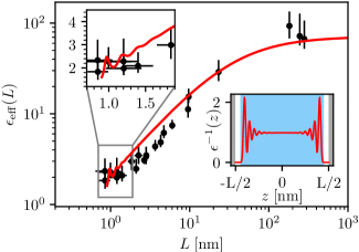
Figure 4: Effective dielectric permittivity $\epsilon_{{\rm eff}}$ of water nanoconfined in a channel of width $L$. Comparison between experimental measurements reproduced from [1] and theoretical model.

Nanoconfined water - We use now this theoretical model to derive the dielectric properties of a confined water layer. The experimental measurements report an effective dielectric permittivity up to $\epsilon_{{\rm eff}}=2$ for a channel of about $1\text{\,}\mathrm{n}\mathrm{m}$.[1] (reported on Fig. 4). The authors suggest the existence in the channel of three water layers of homogeneous dielectric properties: two interfacial layers ($\epsilon=2.1$, thickness: $0.7\text{\,}\mathrm{n}\mathrm{m}$) and a layer of bulk water ($\epsilon=78$). We compute the effective permittivity $\epsilon_{{\rm eff}}=L/\int_{0}^{L}(1-\chi(z))dz$ as a function of $L$ for two graphene surfaces. Our model can be seen as two vacuum gaps and an inhomogeneous water layer. This inhomogeneity is not implemented ad hoc but is the signature of the nonlocal dielectric properties of water, revealed by the boundary conditions. The results are presented in Fig. 4. The model reproduces the experimental measures and catches in particular a non-homogenous behavior of the permittivity as a function of $L$ for small $L$ as shown in the insert that cannot be described by a three homogeneous layer model.[38, 1, 4]

Conclusion - Nanoconfined water is a non-homogeneous dielectric material which properties differ dramatically from the bulk. Water-surface interaction and the bulk properties of the fluid combine to induce specific dielectric profiles. The complexity of this system is captured by a minimal phenomenological Hamiltonian depending on the polarization field and composed of (i) a LG forth order development for a bulk-determined term and (ii) a harmonic surface-water term. We show that the dielectric susceptibility of interfacial water may be strongly affected by the coarse-grained parameters ($\tilde{k}_{m}$, $\tilde{k}_{\rho}$, $\eta$) characterizing local surface-water interaction. It gives a framework to compare graphene and hBN that could be predictive for other surfaces and also to derive the dielectric properties confined water in other geometries, such as nanotubes.[39]